The Low-Redshift Ly Forest toward 3C 273Thanks: Based on observations with (1) the NASA/ESA Hubble Space Telescope,obtained at the Space Telescope Science Institute, which is operated by the Association of Universities for Research in Astronomy, Inc., under NASA contract NAS 05-26555, and (2) the NASA-CNES/ESA Far Ultraviolet Spectroscopic Explorer mission, operated by the Johns Hopkins University, supported by NASA contract NAS 05-32985.
Abstract
We present an analysis of the Ly forest toward 3C 273 from the Space Telescope Imaging Spectrograph at km s-1 resolution, along with re-processed data from the Far Ultraviolet Spectroscopic Explorer. The high UV flux of 3C 273 allows us to probe the weak, low absorbers. The main sample consists of 21 H I absorbers that we could discriminate to a sensitivity of . The redshift density for absorbers with is below the mean for other lines of sight; for , it is consistent with numerical model predictions. The Doppler parameter distribution is consistent with other low samples. We find no evidence for a break in the column density power-law distribution to . A broad Ly absorber (BLA) is within km s-1 and 1.3 local frame Mpc of two galaxies, with an O VI absorber km s-1 away, similarly close to three galaxies and indicating overdense environments. We detect clustering on the km s-1 scale at significance for , consistent with the level predicted from hydrodynamical simulations, and indication for a Ly forest void at . We find at least two components for the Virgo absorber, but the total column is not significantly changed.
Keywords:
cosmology: observations – galaxies: intergalactic medium – quasars: absorption lines1 Introduction
The low redshift Ly forest offers both a challenge and an opportunity to study the physics of the intergalactic medium and its role in galaxy formation and evolution. The challenge is the requirement for space-based UV spectroscopy, which is undergoing a renewal with the installation of COS on HST. The opportunity is to observe absorption systems at small enough distances to be able to relate nearby galaxy characteristics far down the luminosity function. The calculation and interpretation of numerical models using the fluctuating Gunn-Peterson approximation (Croft et al., 1998, e.g) greatly benefit from constraints on the end epoch for absorber distribution functions such as number densities, column densities, Doppler parameters, clustering and relations to galaxies. A consequence of the models is that the low- Ly forest is predicted to harbour a significant fraction of the baryons, as is a hot shocked component (Davé et al., 1999; Cen & Ostriker, 1999; Davé et al., 2001, e.g.). For a given column density, the low- forest is predicted to probe larger mass overdensities than at high redshift, which adds complexity to comparisons of absorber property distribution functions between widely differing epochs.
Exploration of the Ly forest began in earnest with HST observations of the brightest QSO, 3C 273, using the Faint Object Spectrograph (Bahcall et al., 1991) and Goddard High Resolution Spectrograph (Morris et al., 1991), which revealed 5 and 10 Ly absorbers, respectively. The main result was that there were many more low redshift systems than expected from a simple extrapolation from of the decline of the absorber redshift density over time. Concurrently, observations of the galaxy environments around Ly absorbers were made, again with the 3C 273 field among the first to be probed, which revealed a complex relationship between absorbers and galaxies. The absorber-galaxy correlation was found to be stronger than random but not as strong as the galaxy-galaxy correlation (Salzer, 1992; Morris et al., 1993; Stocke et al., 1995; Lanzetta et al., 1995; Shull, Stocke & Penton, 1996; Tripp, Lu & Savage, 1998), a trend which has held up in recent years (Chen et al., 2005; Prochaska et al., 2006, e.g.). Using H I-selected galaxies, however, Ryan-Weber (2006) found the absorber-galaxy correlation even stronger than the galaxy autocorrelation on Mpc scales.
Over the last 17 years, great efforts were made to accumulate observations of a number of low redshift QSOs. A leap in observing efficiency came with the installation of STIS in 1997. Crucial access to higher order Lyman lines was provided by the launch of the Far Ultraviolet Spectroscopic Explorer (FUSE) in 1999. To date, a few hundred low- Ly forest lines have been observed at resolutions down to km s-1. Such works typically involved studies of one to a few sight lines at a time e.g. Williger et al. (2006) (Paper I), but more recently therein large analyses of archival data, including recent works by Lehner et al. (2007a),Danforth & Shull (2008) , and Wakker & Savage (2009). The H I column density distribution shows evidence of a slight steepening at low compared to that at (e.g. Lehner et al., 2007a, and references therein), and also a small increase in the mean Doppler parameter over time. An excess of broad Ly absorbers (BLAs) with km s-1 at is also observed, which is attributed to a larger fraction of warm-hot intergalactic medium (WHIM) gas at low , consistent with model predictions; this population of BLAs is currently the subject of active study (Richter, Fang & Bryan, 2006a; Richter et al., 2006b; Tripp et al., 2008; Wakker & Savage, 2009, e.g.). Recent observational estimates for the baryon contribution of the low- Ly forest are 30% or more (Penton, Shull & Stocke, 2004; Lehner et al., 2007a). Danforth & Shull (2008) argue that low- O VI absorbers reveal 10% of the baryons in warm-hot gas, but Tripp et al. (2008) have shown that many of the O VI lines are well-aligned with narrow H I lines, and in those cases, the O VI absorber properties suggest an origin in cool, photoionised gas. (A similar conclusion is favored by Thom & Chen 2008). Indeed, Oppenheimer & Davé (2009) have argued that most low- O VI systems are photoionised based on their hydrodynamic simulations of large-scale structures. However, some O VI absorbers show strong evidence of hot gas (Tripp et al., 2001; Savage et al., 2005; Narayanan, Wakker & Savage, 2009, e.g.). Larger statistical studies employing more robust diagnostics are required to reliably interpret the natures of O VI absorbers.
3C 273 has always been one of the first extragalactic targets observed with new technology for a variety of astronomical topics (Ulrich et al., 1980, e.g.). In addition to 3C 273 being extremely bright, it also lies behind the Virgo Cluster, which makes it particularly useful for studies of absorber-galaxy relations and the physical conditions in halo and filament gas, from the cluster out to the vicinity of the QSO. In a partial listing of successor projects after the early HST papers cited above, the sight line was the subject of further GHRS observations (Weymann et al., 1995) and a number of galaxy studies relating to absorber environments (Salpeter & Hoffman, 1995; Hoffman et al., 1998; Grogin, Geller, & Huchra, 1998; Impey, Petry, & Flint, 1999, e.g.). Sembach et al. (2001) explored the Ly forest of 3C 273 with FUSE, and Tripp et al. (2002) examined the physical states of two high column density Virgo Cluster absorbers. Rosenberg et al. (2003) compared Virgo metal systems toward RXJ1230.8+0115, which is the nearest bright low redshift QSO (, 55 arcmin away), and concluded that a large scale structure filament may produce correlated absorption.
Preliminary results for km s-1 resolution STIS echelle spectroscopy of 3C 273 were presented by Heap et al. (2002) and Heap et al. (2003). We present a full analysis here, including a coverage of Galactic and IGM absorption system parameters. We also make use of complementary data from FUSE, with recent improvements in data processing, reduction and analysis. The QSO 3C 273 lies at Galactic , , and thus serves as a very useful probe of the Galactic halo. Over wavelengths covered by the Ly forest, our data have per km s-1 pixel with pixels per resolution element at 1200 Å (Dressel et al., 2007), except for small dips at the ends of orders. The superior signal and resolution of our data permit us to probe the low- Ly forest to , which is the best observation done to date, regardless of resolution. This column density limit corresponds to mass overdensities of (Davé et al., 1999; Davé & Tripp, 2001) as calculated from hydrodynamical models in the cold dark matter scenario. Similar mass overdensities at correspond to (though the true density-column density relation is likely complex due to the non-linear growth of large perturbations). The high of our spectrum also allows us to detect BLAs with good efficiency. The study of hot halo gas for the Virgo absorbers along this sight line (Tripp et al., 2002; Tripp et al., 2008) prompted us to verify the component structure of the absorber with the FUSE data. While a number of recent Ly forest publications tend to include more and more sight lines per paper, our focus on the single sight line of 3C 273 merits an in-depth analysis of the Ly forest from a special perspective, due to the high quality of the spectrum and the value added by existing and future deep galaxy surveys in the region.
This paper is organized as follows. We describe the STIS and FUSE observations in § 2. The absorption line selection procedure details are in § 3, as are a list of Galactic absorption lines in the STIS data and an upper limit on C IV absorption for a high H I column density absorber at . We explain our simulations to constrain the probability of feature detection in § 3.4. Our results and discussion for the Ly forest, BLAs and their relation to O VI absorbers and galaxies, clustering and voids, and the Virgo absorber velocity structure are in §4. Our conclusions are summarised in § 5. We adopt a cosmology of km s-1 Mpc-1, and throughout this work.
2 Observations and reductions
2.1 STIS spectra
3C 273 was observed with HST and STIS using guaranteed time from Program 8017 to the STIS Instrument Definition Team (IDT). The instrumental setup used grating E140M for seven orbits (18671 sec) on 2000 May 2 and 2000 June 21-22, with the slit. For the E140M grating, the STIS Instrument Handbook gives a dispersion of /91700 Å pix-1, a FWHM for the line spread function for the slit of 1.4 and 1.3 pixels at 1200 and 1500 Å respectively, and a resolving power for a two-pixel resolution element of 45800.
The data were processed and spectra extracted with calstis and a suite of programs from the STIS ID Team at Goddard Space Flight Center, including corrections for scattered light and hot pixels and customised merging of echelle orders to minimize echelle ripple (written by Don Lindler). We constructed a continuum using a combination of routines from automated autovp (Davé, Dubinski, & Hernquist, 1997) and interactive line_norm routines (D. Lindler), because the regions around emission lines were best done with manual fitting. Longward of our Ly forest sample region, two regions at 1402-1405 and 1425-1430 Å were lost due to vignetting from the STIS repeller wire. The total STIS wavelength coverage is 1142–1709 Å. Redward of 1616 Å, there are five small ( Å) inter-order gaps.
2.2 FUSE spectra
We use FUSE spectra from the principal investigator program P10135. An analysis of the FUSE data was done by Sembach et al. (2001), which employed a customised version of the FUSE pipeline Calfuse 1.8.7. In this study, we used similar techniques and Calfuse 3.1.3. We screened the data for valid photon events, registered the individual spectra by cross-correlating on the interstellar features, and set the zero point by cross referencing with HST data for interstellar lines. Both the FUSE LiF and SiC channel data show some improvement in terms of resolution. In the 2001 reduction, the screening limits for pulse height distribution were (manually) set with care, but in this work, the wider default values were used. The use of these wider values was able to reduce the noise compared to the earlier reduction. Aside from a small stretch in the LiF2 data and cases where a feature fell on a fibre bundle boundary, the velocity scale is generally good to km s-1, save for a few cases where there is an offset of as much as half a resolution element (22-25 km s-1). The SiC backgrounds are good except for SiC1 at Å. We refer the reader to Sembach et al. for further details.
For profile-fitting, we originally used night-only FUSE data; later we tried using all of the data but found no significant improvement in the results. Continua for the FUSE spectra were created using interactive line_norm routines. We permitted velocity offsets as a free parameter on the order of the FUSE uncertainties as needed to improve individual fits. Absorption system parameters presented in this paper use the night-only data.
3 Absorption Lines
3.1 Selection
Absorption line selection was a multi-step process. We began the process by pre-selecting an inclusive line list using a series of selection criteria based on significance. Our initial step was to make a preliminary selection of absorption features from the summed STIS data down to the significance level with a Gaussian filter based on the autovp routine, with half- widths of 8, 12, 16, and 20 pixels. The large width provides sensitivity to broad Ly absorbers and partially resolved complexes. As a further preliminary (and complementary) constraint, we then only included significant features within the regions flagged as significant in absorption with a simple equivalent width significance criterion, based on a threshold for contiguous pixels below the continuum; such a criterion is more sensitive to narrow absorbers. Whenever possible, we confirmed spectral features by using the FUSE data. In particular, all (9 out of 9) absorbers with over were confirmed by inspection of Ly data, and Ly inspections showed no useful information for lower column density Ly forest systems. The selection algorithm to this point was designed to be largely objective and repeatable, aside from continuum fitting around emission features. We then visually checked each absorption feature to avoid including noise spikes or potential continuum errors.
We subsequently tested the effectiveness of this selection technique by subjecting it to simulated spectra with similar resolution to the data to determine the 80% detection probability based on a grid of Doppler parameters, H I column densities and values. Details are in §3.3 below. The decrease in detection probability drops steeply from nearly 100% to nearly zero over 0.1 dex in column density for a given and Doppler parameter, which enables straightforward determinations of the 80% detection efficiency to 0.05 dex accuracy. Such a steep decline is not unreasonable given that the absorbers are of such low column density () that they are well on the linear part of the curve of growth. Their equivalent widths change little over the limited range of Doppler parameters and S/N (factors of 2) which we explored, and their velocity widths also only vary over a small interval. Therefore, when detecting weak but significant features relying in part on a boxcar approximation to an absorption profile, a range of 0.3 dex (factor of 2) in column density would be a large range to expect a uniform detection threshold probability.
We made a concentrated effort to understand the rate of false detections, due to our desire to probe as deeply as possible down the H I column density distribution. Therefore, as an additional test, we examined the spectrum km s-1 redward of the QSO’s Ly emission all the way to the red end of the STIS data (1710 Å) for unidentified absorption features to test for the frequency of appearance of potential spurious features. The most significant one at 1667.9 Å had a significance , which was well below our preliminary selection threshold. It would have Ly fitting parameters of and Doppler parameter . The relatively large (47%) error in would make it unlikely to be considered a reliable Ly absorber, even if it had somehow been included in our preliminary absorber list. The feature does not correspond to any plausible metal line for any Ly absorber in our sample. The final STIS E140M spectrum of 3C 273, with absorption systems marked, is shown in Figure 1.
3.2 Profile fitting technique
The data were profile-fitted with vpfit11 1 http://www.ast.cam.ac.uk/rfc/vpfit.html (Webb, 1987) using Voigt profiles convolved with the local STIS line spread function (LSF) taken from the STIS Instrument Handbook. Oscillator strengths are from the vpfit atomic data list (2004 Dec. version), based on Morton (2003). Multiple transitions were used for simultaneous fits whenever they could improve constraints on column densities and Doppler parameters. We also used, as necessary, the vpfit capabilities to allow for offsets in the local continuum level and in velocity for each spectral interval used in a fit. The latter would in particular compensate for small velocity uncertainties in the FUSE data.


3.3 Simulated spectra to determine detection probabilities
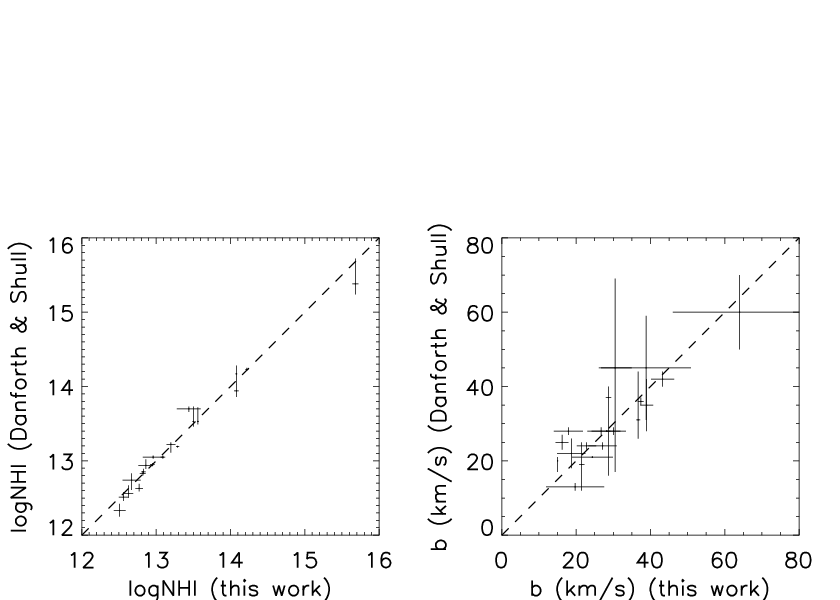
To give us a clearer picture of our Ly line detection probability as a function of S/N ratio and Doppler parameter, we analysed 880 simulated Ly lines. The emphasis here is on characterizing the detection and recovery of of weak absorbers and their line parameters, because the 3C 273 data uniquely probe the low end of the Ly forest column density distribution. The simulations were in addition to the ones done for PKS 0405-123 described in Paper I. The simulated lines were generated using the STIS LSF and a grid of values for , Doppler parameter and H I column density. The values were set to either 20 or 40 per pixel, Doppler parameters were set to ranges with averages of 17.5, 22.2 or 24.7 and 35.0 km s-1, and the input log values varied over 12.21–12.80 for S/N=20 and 11.85–12.55 for . The simulated spectra were continuum-normalised, so any errors, systematic or random, involving continuum fitting are not reflected in the subsequent simulation analysis. There were also no noise spikes inserted into the spectra. We calculated statistics comparing the line parameters for simulated lines which were successfully recovered vs. the input values. Results for the various combinations of input S/N ratio and Doppler parameter are shown in Tables 1 and 2. The mean recovered measured Doppler parameters and column densities match the mean input values within the mean of the profile fitting errors. The marginal tendency for the narrowest lines to be recovered with higher Doppler parameters is likely due to the effects of noise broadening input for features near the detection limit for recovered lines; noise which would make lines narrower presumably would cause the features to drop below the (essentially equivalent width-defined) detection threshold (Rauch et al., 1993). The recovery of the line parameters (e.g., the -value) was found to be even better for stronger lines detected at high significance, up until the point where the H I lines start to saturate badly. The spurious detection rate is % among all the simulations above the 80% detection probability threshold, and thus is not considered significant. The boundary of the 80% detection probability threshold can be parametrically fitted by , where snr is the signal to noise ratio (S/N) per pixel, and established using simulated lines with km s-1. The process was adapted from the method used in Paper I. 22 2 The coefficient of 0.27 for for this paper is % lower than the analogous value of 0.34 from Paper I, and the snr coefficient in this work is 11% higher. The difference in the coefficient may be caused by the relatively lower column density range used for the input lines for this study, in that the limited Doppler parameter range used affects the equivalent widths and thus detectibility of the lines less strongly. The difference in the snr coefficient may also stem from a similar cause, or from either the higher S/N in the 3C 273 data and/or the use of only two input S/N values in this study, 20 and 40. In comparison, for PKS 0405-123, we used three evenly distributed in log space over the range we tested. The difference in results between a coefficient of 1.12 and 1.00 (without adjusting the other coefficients) is only 0.03 dex for our minimum S/N of 21, and the current value of 1.12 leads to a more conservative detection threshold as . We do not believe that the results of this paper are significantly affected by the difference in parametrization.33 3 We will publish an erratum for Paper I (Williger et al., in prep.). In that work, a subset of absorbers principally below the 80% detection threshold had erroneously high calculated significance because the contribution of continuum uncertainties to the total equivalent width errors was not included in the software. We consider this parametrization useful to determine our 80% detection threshold over a Doppler parameter range of 10-40 km s-1, with the bounds based both on our simulations and to compare with the analysis of Lehner et al. (2007a).
| Doppler parameter (km s-1) | Doppler parameter (km s-1) | Doppler parameter (km s-1) | ||||
|---|---|---|---|---|---|---|
| inputb | recoveredc | inputb | recoveredc | inputb | recoveredc | |
| 20 | ||||||
| 40 | ||||||
a Signal to noise ratio per pixel in simulated STIS spectra.
b Mean and first order about the mean for input Doppler parameters in simulations which were recovered.
The simulations for S/N=20, km s-1, were made from a distribution made at
the beginning of our analysis, with a much
wider standard deviation (5.5 km s-1) in input than the others, hence the difference with the
km s-1 case (the geometric mean of 17.5 and 35.0).
The results between the two cases are within the scatter, so we
did not make a simulation run with S/N=20, km s-1.
c Mean and first order about the mean for recovered Doppler parameters in simulations,
with the mean in the formal profile fitting errors in parentheses. The mean recovered Doppler
parameters are all within the mean profile fitting errors of the input values.
| Dopplerb | |||
|---|---|---|---|
| parameter (km s-1) | inputc | recoveredd | |
| 20 | 17.5 | ||
| 40 | 17.5 | ||
| 20 | 22.2 | ||
| 40 | 24.7 | ||
| 20 | 35.0 | ||
| 40 | 35.0 | ||
a Signal to noise ratio per pixel in simulated STIS spectrum.
b Simulation sets are specified by input Doppler parameter.
c Mean and first order about the mean for input log H I column densities in simulations which were recovered.
d Mean and first order about the mean for recovered log H I column densities in simulations,
with the mean in the formal profile fitting errors in parentheses.
3.4 Profile fits to data
In addition to H I lines, we find and list, for completeness, profile fits or column density limits (Savage & Sembach, 1991, from vpfit or from the apparent optical depth method,) for a number of Galactic and intervening metal absorber species.
Galactic absorption. We find Galactic absorption from H I, C I, C I∗, C II, C II∗, C IV; N I, N V, O I, Mg II, Al II, Si II, Si III, Si IV, P II, S II, S III, Mn II, Fe II, Ni II. Galactic absorption ranges over km s-1, consistent with the high velocity absorption found in the FUSE spectrum by Sembach et al. (2001). A complete list of absorber profile fitting parameters is in Table 3. In the case of saturated lines, we calculate lower limits by the apparent optical depth method Savage & Sembach (1991), which are consistent with the results of Sembach et al. (2001). The maximum optical depth used is a function of local S/N and continuum error ( per pixel), in which both effects contribute to similar degrees. For the 3C 273 data, .
For two of the highest column density systems toward 3C 273, members of this collaboration and others have investigated metallicity limits and undertaken studies in the low IGM (Davé et al., 2001; Tripp et al., 2002; Stocke et al., 2007; Tripp et al., 2008, e.g.). Such low redshift, high column density absorbers are extremely useful for comparison with nearby low luminosity faint galaxies e.g. the dwarf galaxy found 71 kpc away from the Virgo cluster absorber (Stocke et al., 2004). For completeness and comparison with their results, we provide here upper limits for C IV for each of these absorbers, and for a sum of the C IV regions over a consistent km s-1, using the above-mentioned apparent optical depth method. The absorber was found by Tripp et al. to have rest equivalent width mÅ over km s-1, or assuming an absorber on the linear part of the curve of growth. Stocke et al. found (3) for the system over km s-1. We measured an upper limit for the absorber of mÅ () over km s-1, or .44 4 The difference in upper limits arises in that the Stocke et al. limit is for one resolution element, whereas our limit is over 200 km s-1 in velocity space or resolution elements, to be consistent with the Tripp et al. measurement. We stacked the data for the two systems and found mÅ () km s-1, or .55 5 This limit is slightly tighter than the 24 mÅ result expected from stacking the spectra according to the inverse square of the S/N. The difference in our result may be from the way each team determined the local continuum and S/N, in particular as these were measured over two different velocity intervals.
4 Results and discussion
4.1 Ly absorber statistics
We use our detection probability results to define a sample for , which is approximately the 80% detection threshold for our worst case in the Ly forest and assuming a Doppler parameter of km s-1 66 6 Note that by choosing km s-1, this leads to a higher, more conservative 80% probability detection threshold in by 0.06 dex than by choosing km s-1, which is typical of high resolution, high Ly forest data. We prefer to be conservative, given the possibility of unresolved blends caused by our limits in the achievable . This choice of does not affect our subsequent analysis in any way except for this small change in the threshold for .. This low H I column density threshold sample covers the range and contains 21 Ly absorbers. We excluded absorbers within km s-1 of 3C 273 to minimize the impact of the proximity effect (Murdoch et al., 1986; Bajtlik, Duncan & Ostriker, 1988).
In later subsections, we will discuss in detail our examinations of the Ly forest Doppler parameter distribution, redshift density , broad line population and column density distribution. We do not distinguish between metal and Ly-only systems in this analysis, the same approach as in Paper I. Metals have been found in progressively lower column density Ly systems at (e.g. Cowie et al., 1995; Songaila & Cowie, 1996; Pettini et al., 2001, and references therein). Also, the absorbers we can detect at low redshift probably are best related to large density perturbations at (Schaye, 2001, e.g.) which are commonly associated with metals. Finally, the limited wavelength range of the data does not permit a uniform coverage for metal detection (in particular for C IV, limited to ).
| species | errora | (km s-1) | errora | (km s-1) | errora | lines (Å)c,f,g | |
|---|---|---|---|---|---|---|---|
| O I | -0.000451 | 0.000041 | 61.5 | 22.1 | 13.55 | 0.12 | 1302 |
| C IV | -0.000240 | 0.000003 | 11.6 | 1.8 | 13.45 | 0.09 | 1548,1550 |
| Si IV | -0.000230 | 0.000003 | 7.9 | 1.4 | 12.57 | 0.06 | 1393,1402 |
| Si II | -0.000224 | … | … | … | … | 1190,1193,1260,1304,1526 | |
| O I | -0.000220 | … | … | … | … | 1302 | |
| S II | -0.000159 | 0.000016 | 10.1 | 4.9 | 13.74 | 0.24 | 1250,1253,1259 |
| Si IV | -0.000103 | … | … | … | … | 1393,1402 | |
| S III | -0.000084 | … | … | … | … | 1190 | |
| Fe II | -0.000071 | … | … | … | … | 1608 | |
| N I | -0.000067 | … | … | … | … | 1199,1200 | |
| Mn II | -0.000067 | … | 14.2 | … | 12.60 | 0.19 | 1197,1199,1201d |
| Ni II | -0.000067 | 0.000004 | 22.3 | 1.7 | 13.73 | 0.03 | 1317,1370,1454 |
| C II | -0.000067 | … | … | … | … | 1334 | |
| C IV | -0.000066 | 0.000003 | … | … | … | 1548,1550 | |
| S II | -0.000060 | … | … | … | … | 1250,1253,1259 | |
| Si IV | -0.000060 | 0.000012 | 48.8 | 2.3 | 13.73 | 0.04 | 1393,1402 |
| P II | -0.000056 | 0.000017 | 29.1 | 7.5 | 13.69 | 0.10 | 1152,1532 |
| Si II | -0.000067 | … | … | … | … | 1190,1193,1260,1304,1526 | |
| C II* | -0.000045 | 0.000002 | 14.3 | 0.8 | 13.83 | 0.02 | 1335 |
| C I* | -0.000044 | 0.000000 | 9.1 | 0.0 | 12.24 | 0.26 | 1561,1656,1657e |
| C I | -0.000044 | 0.000005 | 9.1 | 2.4 | 12.79 | 0.07 | 1277,1280,1328,1560,1656 |
| Si III | -0.000042 | … | … | … | … | 1206 | |
| Mg II | -0.000038 | 0.000012 | 27.9 | 5.1 | 15.43 | 0.06 | 1239,1240 |
| N V | -0.000037 | 0.000005 | 59.8 | 2.2 | 13.93 | 0.01 | 1238,1242 |
| Al II | -0.000033 | … | … | … | … | 1670 | |
| H I | -0.000027 | 0.000005 | … | … | 20.23 | 0.00 | Ly |
| O I | -0.000025 | … | … | … | … | 1302 | |
| Fe II | 0.000068 | … | … | … | … | 1608 | |
| N I | 0.000068 | … | … | … | … | 1199,1200 | |
| Mn II | 0.000068 | … | 4.4 | … | 12.63 | 0.18 | 1199,1200d |
| S II | 0.000069 | 0.000001 | 9.4 | 0.6 | 14.75 | 0.01 | 1250,1253,1259 |
| Ni II | 0.000074 | 0.000004 | 13.3 | 2.0 | 13.41 | 0.05 | 1317,1370 |
| C II* | 0.000078 | 0.000001 | 7.6 | 0.7 | 13.73 | 0.02 | 1335 |
| C I | 0.000081 | 0.000001 | 6.4 | 0.7 | 13.27 | 0.02 | 1277,1280,1328,1560,1656 |
| C I* | 0.000081 | 0.000000 | 6.4 | 0.0 | 12.67 | 0.09 | 1561,1656,1657e |
| C IV | 0.000138 | 0.000012 | 20.7 | 4.4 | 13.32 | 0.15 | 1548,1550 |
| Si II | 0.000159 | … | … | … | … | 1190,1193,1260,1304,1526 | |
| S II | 0.000171 | 0.000009 | 1.3 | 4.1 | 13.13 | 0.21 | 1250,1253,1259 |
| O I | 0.000190 | 0.000015 | 13.0 | 5.7 | 13.41 | 0.19 | 1302 |
| C II | 0.000206 | … | … | … | … | 1334 | |
| Si IV | 0.000225 | 0.000020 | 15.2 | 11.6 | 12.21 | 0.56 | 1393 |
a Errors are 1 , and assume that the component structure is correct.
b Upper limits from vpfit or the apparent optical depth method of Savage & Sembach (1991).
c Lines used in profile fits.
d Mn II tied in redshift and Doppler parameter to N I.
e C I∗ tied in redshift and Doppler parameter to C I.
f We find an unidentified feature at 1149.3 Å (also in the FUSE data).
g We find a weak feature at 1304.74 Å to be an artefact just redward of an echelle
overlap region, and not securely identifiable with any plausible ISM or IGM absorption.
4.1.1 Redshift density and intervening absorber list
Measuring the Ly forest redshift density has been one of the biggest goals among HST Key Projects, and initially yielded surprising results. From among the first results with FOS Bahcall et al. (1991) and GHRS Morris et al. (1991) toward 3C 273, the Ly redshift density was found to be higher than expected from extrapolations of ground-based data. To compare results with recent high resolution data in the literature, we present data for and , using the restrictions of km s-1, and errors in and of % for both 3C 273 and the literature values (Lehner et al., 2007a, to use the same criteria as). We also present results for . Due to the low redshift of 3C 273, the data are unaffected by losses from inter-order gaps in the STIS data. Similar to our analysis in Paper I, we excluded pixels from metal absorption with optical depth , which removed from the samples for and .77 7 Metal absorption from pixels with can also reduce the probability of detection an IGM Ly absorber, but less so than those with . The value of is a compromise to eliminate the worst metal absorption regions without losing too many pixels with recoverable Ly data. Other factors such as multiple transitions from a metal ion can mitigate the masking effect of metal absorption. For example, we recovered the presence of Ly absorption blended with Galactic Si IV. This left an unblocked redshift path of for and for . In an analogous way, we find for (which requires a smaller, higher S/N subset of the data). The absorption distance (Tytler, 1987), using the prescription of Lehner et al. (2007a), which will be used for comparing H I column density distributions in the next section.
We list in Table 4 intervening H I and related metal redshifts, column densities and Doppler parameters, including several systems either outside of the unblocked redshift intervals corresponding to the sensitivities mentioned above, or at which nevertheless fulfill all of the other selection criteria. We show in Figure 2 the Doppler parameters and H I and column densities for all Ly forest systems that we detected using the procedure described in § 3, overlaid with the our parametrically fitted 80% detection sensitivities.
A. High column density lines
For absorbers with from among our full sample of 21 systems, we find four over the interval (). If we restrict our sample to km s-1 and errors in and to %, the number reduces to 3 (). The difference arises from the lower component of the Virgo absorber, which has a column density error of a factor of 2 and is examined in more detail in § 4.4. We compare our results with the literature (Fig. 3), and illustrate the scatter for seven other sight lines with contiguous redshift coverage of from Williger et al. (2006, PKS 0405-123, = Δ z 0.413 ),88 8 We corrected the line list for spurious absorbers, and will publish the updated list in an erratum (Williger et al. 2009, in prep.). Sembach et al. (2004, PKS1116+215, = Δ z 0.133 ) and Richter et al. (2004, PG 1259+593, = Δ z 0.247 ), Lehner et al. (2007a, HE0226-4110, H1821+643 and PG0953+415, = Δ z 0.397, 0.238, 0.202 respectively), Aracil et al. (2006, HS 0624+6907, = Δ z 0.329 ). The redshift density is marginally high (similar to PKS 0405-123) but still consistent with other measurements from the literature shown in Fig. 3 (right panel), similarly selected for km s-1and with errors in and of %. The small number statistics and large cosmic scatter ( dex in for individual sight lines) make make further analysis difficult without larger samples. The cosmic scatter range appears to persist to . To illustrate the effect of the restriction in and in the errors, we also included the redshift density from the large, lower resolution sample of Weymann et al. (1998), which was selected on the basis of rest equivalent width and cannot filter out km s-1 systems, and is higher than our result. We note that the determination of Wakker & Savage (2009) is consistent with the Weymann et al. result, as both studies relied on equivalent widths rather than column densities with restrictions on the Doppler parameters. The redshift densities for restricted, high resolution sight lines are in general a factor of lower than the analogous sight lines.

| species | errora | (km s-1) | errora | errora | lines (Å)b,c | ||
|---|---|---|---|---|---|---|---|
| H I | 0.002630 | 0.000039 | 125.8 | 44.9 | 13.04 | 0.14 | Ly |
| H I | 0.003369 | 0.000002 | 37.4 | 0.8 | 14.22 | 0.02 | Ly |
| H I | 0.005251 | 0.000021 | 26.1 | 1.3 | 14.33 | 0.31 | Ly |
| Si II | 0.005266 | 0.000005 | 5.2 | 2.6 | 11.78 | 0.09 | 1190,1260 |
| H I | 0.005295 | … | 15.0 | 0.0 | 15.68 | 0.04 | Ly |
| C II | 0.005295 | … | 8.6 | 0.1 | 12.80 | 0.07 | 1036,1334 |
| Si III | 0.005295 | 0.000002 | 8.2 | 2.1 | 12.36 | 0.07 | 1206, sets for Si III, H I |
| H I | 0.007165 | 0.000029 | 38.8 | 12.1 | 12.67 | 0.12 | Ly |
| H I | 0.007588 | 0.000037 | 64.0 | 18.0 | 12.86 | 0.10 | Ly |
| H I | 0.026225 | 0.000006 | 26.7 | 2.5 | 12.95 | 0.03 | Ly |
| H I | 0.029348 | 0.000028 | 17.1 | 6.4 | 12.77 | 0.28 | Ly |
| H I | 0.029471 | 0.000008 | 19.7 | 7.8 | 13.24 | 0.16 | Ly |
| H I | 0.029578 | 0.000016 | 11.6 | 5.9 | 12.63 | 0.30 | Ly |
| H I | 0.032798 | 0.000006 | 22.8 | 2.6 | 12.82 | 0.04 | Ly |
| H I | 0.039373 | 0.000012 | 28.2 | 5.2 | 12.63 | 0.06 | Ly |
| H I | 0.046639 | 0.000013 | 24.4 | 5.5 | 12.51 | 0.08 | Ly |
| H I | 0.049000 | 0.000002 | 28.7 | 0.7 | 13.56 | 0.01 | Ly |
| H I | 0.049953 | 0.000004 | 16.2 | 1.7 | 12.83 | 0.03 | Ly |
| H I | 0.054399 | 0.000017 | 23.6 | 6.6 | 12.41 | 0.10 | Ly |
| H I | 0.063510 | 0.000018 | 17.9 | 3.9 | 12.96 | 0.14 | Ly |
| H I | 0.064078 | 0.000025 | 39.8 | 10.9 | 12.62 | 0.09 | Ly |
| H I | 0.066548 | 0.000001 | 36.7 | 0.5 | 14.08 | 0.01 | Ly |
| H I | 0.073738 | 0.000034 | 64.0 | 15.0 | 12.74 | 0.08 | Ly |
| H I | 0.074286 | 0.000033 | 51.2 | 13.8 | 12.62 | 0.10 | Ly |
| H I | 0.075377 | 0.000009 | 27.1 | 3.8 | 12.77 | 0.05 | Ly |
| H I | 0.085882 | 0.000028 | 34.9 | 11.3 | 12.41 | 0.11 | Ly |
| H I | 0.087632 | 0.000008 | 43.3 | 3.1 | 13.09 | 0.03 | Ly |
| H I | 0.089746 | 0.000012 | 30.5 | 4.4 | 13.08 | 0.06 | Ly |
| H I | 0.089898 | 0.000009 | 12.8 | 4.3 | 12.60 | 0.15 | Ly |
| H I | 0.090110 | 0.000004 | 30.1 | 1.8 | 13.29 | 0.02 | Ly |
| H I | 0.109141 | 0.000015 | 18.8 | 6.2 | 12.33 | 0.11 | Ly |
| H I | 0.109380 | 0.000009 | 18.7 | 3.8 | 12.56 | 0.06 | Ly |
| O VI | 0.12003 | … | … | … | 13.45 | 0.10 | 1032,1038f |
| H I | 0.120041 | 0.000002 | 21.5 | 0.7 | 13.50 | 0.01 | Ly |
| H I | 0.141676 | 0.000024 | 32.6 | 9.6 | 12.36 | 0.10 | Ly |
| H I | 0.146575 | 0.000005 | 39.0 | 1.7 | 14.08 | 0.03 | Ly |
| H I | 0.150204 | 0.000021 | 32.9 | 7.8 | 12.37 | 0.08 | Ly |
| H I | 0.157787 | 0.000006 | 21.5 | 2.1 | 12.63 | 0.03 | Ly |
| O VI | 0.15779 | … | … | … | 13.39 | 0.11 | 1032f |
a Errors are 1 , and assume that the component structure is correct.
b Lines used in profile fits.
c We find an unidentified feature at 1149.3 Å (also in the FUSE data).
d Inclusion of Ly makes no significant difference to the fit.
e Ly absorption confirmed by Ly.
f Tripp et al. (2008).

B. Medium column density lines
In both in our full sample and our restricted sample for km s-1 and errors in and of %, we find 4 absorbers over the interval with (). We compare our results with the literature, and illustrate the scatter for seven other sight lines with contiguous redshift coverage of from Williger et al. (2006, PKS 0405-123, = Δ z 0.212 ), Sembach et al. (2004, PKS1116+215, = Δ z 0.133 ) and Richter et al. (2004, PG 1259+593, = Δ z 0.247 ), Lehner et al. (2007a, HE0226-4110, H1821+643 and PG0953+415, = Δ z 0.294, 0.238, 0.202 respectively), Aracil et al. (2006, HS 0624+6907, = Δ z 0.329 ). We note that Lehner et al. estimated completeness to , so the line densities for the three objects from that study should be a lower limit. For PKS 0405-123, we use a revised line list for PKS 0405-123 (Williger et al., in prep.) and the redshift interval known to be complete to (Paper I). We consulted with N. Lehner about the signal-to-noise characteristics of the other sight lines in their work (private communication, 2007). We have split the HS 0624+6907 sight line into high and low halves to keep the redshift intervals to similar length compared to that of 3C 273. Results are plotted in Fig. 3 (left panel).
The cosmic scatter covers about 0.2 dex in at , for all sight lines except 3C 273, which is below the mean of the other seven sight lines. For comparison, the redshift density of Wakker & Savage of (based on their fig. 5b) is just consistent with the maximum of the individual sight line values, again possibly showing the difference in redshift density using equivalent widths vs. column densities with restricted Doppler parameters. At , a larger sample (Janknecht et al., 2006) indicates a cosmic scatter range of 0.35 dex which spans both the 3C 273 value and the other seven low sight lines, so the 3C 273 sight line may simply represent the lower end of the redshift density range. The high signal and high resolution in the data here make it unlikely that blending and noise effects are mainly responsible for the paucity of Ly forest lines toward 3C 273 in this column density range. The Cosmic Origins Spectrograph should reveal more definitively whether is representative of one of the sparsest parts of the Ly forest, or if even more poorly populated sight lines exist.
C. Low column density lines
Given the very high signal-to-noise ratio in the 3C 273 data, we also calculate the redshift density for . We find 21 absorbers above this threshold over , for . To compare the 3C 273 sample to the much larger observational data set of (Lehner et al., 2007a), we consider separately those systems with errors in Doppler parameter and under 40% (based on the lower limit errors for ) and km s-1. These criteria focus the sample on relatively cool IGM gas by excluding broad Ly systems (Richter et al., 2006a; Richter et al., 2006b, BLAs, e.g.), which are interpreted as the signatures of physically distinct low- hot IGM gas. The restricted 3C 273 sample is 18 systems (), which consistent to in redshift density with the full sample.
There are few comparisons down to a threshold of for absorbers at low . Observationally, Danforth & Shull (2008) found for (see their fig. 3), which is below our value of , and Wakker & Savage (2009) determined for , which is consistent with our value. These results could be understood in that the weakest lines in the sample dominate the number counts, based on the column density distribution, and should affect an equivalent width based sample (such as Wakker & Savage) less than a sample with a higher column density floor of . From numerical models, Paschos et al. (2009) calculated for the same H I threshold at , which is consistent with our measurements to . Less directly, at , our H I column density threshold corresponds to overdensities of (Davé et al., 1999; Davé & Tripp, 2001) as calculated from hydrodynamical models in the cold dark matter scenario. At , the same overdensity level corresponds to , a rough estimate for which can be read from the right panel of Fig. 3: . Our results are therefore consistent with overdensities of within . We caution that the correspondence of overdensity and may only result from the considered density perturbations being weak, as non-linear growth would be expected over time to skew the overdensity distribution to high values; the low IGM is relatively complex, containing a significant fraction of shock-heated gas (which is related to the BLA population).
The observation of many more sight lines with COS would likely reveal better the extent of cosmic scatter, and provide further comparisons between the Ly forest and galaxy environments e.g. Chen et al. (2005). In particular, COS could provide a large increase in sight lines probed to , though at lower resolution than this study.
4.1.2 Doppler parameter distribution
The Doppler parameter distribution for the entire sample of 21 absorbers has mean, median and standard deviation of 28, 27, 13 km s-1, respectively (Fig. 4). In the same manner as Paper I, we tested whether weak line blending is the cause. We divided the strong sample into high and low H I column density halves, which occurs at , and performed a Kolmogorov-Smirnov test to determine the likelihood that the Doppler parameters are drawn from the same distribution. The probability that the samples are drawn from the same distribution is . The closest observed Ly forest absorber pair in velocity space is km s-1 (between ), or 4-5 times the resolution of the STIS data. The next closest pair is km s-1. This can be compared to the mean velocity interval expected between absorbers (in the absence of clustering, which is expected to be weak and shows no evidence to the contrary, § 4.3) of km s-1, based on our value of for over . We would then expect to first approximation that there is a 0.5% chance of an absorber randomly being km s-1 from another. At such a velocity difference, the lines could potentially be unresolved, depending on the local S/N and the line column densities and Doppler parameters, with the greatest possibility of blending for broad, shallow lines in relatively noisy parts of the data. For the high S/N in the 3C 273 data and the km s-1 absorbers with % errors upon which we are focused, we infer that line blending is not significant for the Ly forest toward 3C 273.
We compared results with the much larger low sample of Lehner et al. (2007a). They restricted their sample to km s-1, to correct for the non-Gaussianity of the Doppler parameter distribution. If we make the same restriction for our data, the sample would have 18 absorbers, with mean, median and standard deviation 24, 24 and 8 km s-1. Lehner et al. (2007a) found values of 27, 27 and 8 km s-1, which is consistent with our results. The , sample of Shull et al. (2000) is also consistent (mean, median, standard deviation 31, 28, 7 km s-1 respectively). Finally, our km s-1 sample is in accord with the Doppler parameter mean of Davé & Tripp (2001) (25 km s-1), which is complete for and includes absorbers down to , and thus shows agreement with their comparison model of a -dominated CDM universe (Davé et al., 1999), and again with the more recent simulations of Paschos et al. (2009).

4.1.3 Column density distribution
Observations suggest (Kim et al., 2002; Misawa et al., 2007, e.g.) and simulations predict (Paschos et al., 2009, e.g.) that the column density distribution should steepen at lower redshift for , which would be consistent with a systematic decrease of column densities over time for overdensities of a given strength. Our data can help to investigate this trend, by uniquely probing the very lowest H I column densities in the Ly forest at low . However, given the small sample size and limited number of absorbers with , we cannot obtain a good slope constraint using just our data, in the framework of the commonly adopted parametric form . Therefore, we employ additional data from the literature to provide a larger comparison sample (larger ), with the majority of absorbers at higher to extend the column density range. We used the Ly forest sample of (Lehner et al., 2007a), which contains 270 Ly systems at , covering absorption distance , and a stated completeness to . They calculated the differential column density distribution for a subsample with km s-1, and errors in and to %, for a total of 132 absorbers. If we select from our sample in a way that is consistent with these rules, the number of included 3C 273 absorbers at is reduced to a subsample of 11. We calculate a maximum likelihood fit of for the Lehner et al. subsample over , with the distribution consistent with a power law to (Kolmogorov-Smirnov probability ). This is consistent with the Lehner et al. value of . We wish to know whether the weakest absorbers below the completeness limit of Lehner et al. are consistent with a single power law distribution. The 3C 273 sample would comprise only 7.6% of a combined sample with the Lehner et al. data, over only 4.9% of the absorption distance, so it would not contribute much weight to a combined sample. We therefore simply extrapolate our best single power law fit for the Lehner et al. subsample, and plot two data points from the complete 3C 273 sample covering in Fig. 5. The largest deviation shown by the 3C 273 data is in the bin, which is within 0.8 of the extrapolated fit. The low column density end of the column density distribution is thus consistent with that at .
We can probe to 0.2 dex lower column density by correcting for the probability of detection at of %. Using the same selection criteria as Lehner et al. (2007a), there are 3 absorbers at toward 3C 273 in this extended column density range. We plot both the observed point, which shows signs of a turnover in , and a factor of two correction, which is still consistent to at within the extrapolated slope from Lehner et al..
Penton et al. (2004) found (consistent to with our results) over at , based on rest equivalent widths and an assumed Doppler parameter of km s-1. Davé & Tripp (2001) used simulations to correct for incompleteness to show no break in the H I column density distribution to , and calculated a consistent slope to our value.

4.2 Broad lines
Broad Ly absorbers (BLAs), with km s-1, have been a subject of interest in the past few years (e.g. Bowen et al., 2002; Penton et al., 2004; Richter et al., 2004; Sembach et al., 2004; Richter et al., 2006a; Richter et al., 2006b; Wakker & Savage, 2009, and references therein), because they may be the sign of a significant reservoir of warm-hot IGM (WHIM) gas. Following the convention of Richter et al., we use a sensitivity limit of
| (1) |
using the signal to noise ratio per (their) 10 km s-1 resolution element in the above expression. This yields given our minimum signal to noise ratio per pixel of in the Ly forest, pixel resolution elements and 3.2 km s-1 pixel size. Our BLA sample contains three Ly absorbers in total ( 0.07374, 0.07429, 0.08763), using the continuum generated by autovp plus manual modifications around emission lines, and the compound feature detection algorithm. Assigning reliability to BLA detections can involve subjectivity, due to the nature of echelle spectra and variety of detection and continuum fitting techniques. Blending, low S/N ratio, kinematic flows, Hubble broadening and continuum uncertainties could be responsible for up to 50% of BLAs. To keep some subjective standards consistent between different studies, we had one co-author (KS), a member of several collaborations which have studied BLAs, examine the BLA candidates. He determined the absorber to be consistent with some “reliable” samples of recent studies of BLAs e.g. Lehner et al. (2007a). Using this identification to divide the BLA sample into “total” and “reliable”, we find for the total BLA sample and for the reliable BLA, using a pathlength of (Fig. 6). These are within of the values for the total and high quality samples in fig. 2 of Richter et al. (2006a) ( and 15 for total and reliable systems, respectively), which were based on simulated spectra drawn from hydrodynamical simulations.

Given that the 3C 273 sight line is covered by the Sloan Digital Sky Survey spectroscopic galaxy catalogue (Adelman-McCarthy et al., 2008, DR6,), we examined the galaxy environment of all BLAs and O VI systems beyond Virgo (Virgo systems being studied in Tripp et al., 2002; Stocke et al., 2006; Wakker & Savage, 2009, , for example) and not in the 3C 273 host cluster. The one secure BLA and one O VI system each have several listed galaxies with spectroscopic redshifts within 1.5 comoving Mpc impact parameter and km s-1. Their H I redshifts of and correspond to a line of sight distance of 9.8 local frame Mpc.
The BLA has 2 galaxies with spectroscopic redshifts from the SDSS within 1.3 local frame Mpc perpendicular to the line of sight ( plane) and km s-1 ( axis) (Adelman-McCarthy et al., 2008). The next nearest galaxy in the plane of the sky, in increasing velocity space difference, is 2MASX J12271948+0200408 ( local Mpc, , km s-1). The next closest galaxies within 1.6 local Mpc on the sky are three at , which are close in redshift to the O VI system (see below). We chose 10,000 random points at over in declination and in right ascension, which contains 1825 galaxies allowing a border. The SDSS spectroscopic sample covers in Petrosian magnitude, which corresponds to over (Blanton et al., 2001; Nakamura et al., 2003, ). By using the SDSS as its own control sample, systematic undercounting of dense regions due the maintenance of a minimum fiber distance should affect both the observed and the control samples similarly. We found that a randomly placed absorber would have at least 2 SDSS galaxies within 1.3 Mpc and km s-1 with a probability of , using the above search regions and varying the redshift limits by . There is a third galaxy with a redshift in the NASA Extragalactic Database but not in the SDSS, LDTA 139870, which is 2.2 local frame Mpc from the line of sight with km s-1; if it were in the SDSS, the random probability of finding three galaxies within 2.2 Mpc would be the same.
The O VI absorber (Tripp et al., 2008, ,) has 3 SDSS galaxies within 1.6 local frame Mpc perpendicular to the line of sight and km s-1. The next closest galaxies within 2.6 local Mpc on the sky are the three at discussed with the BLA above, and 2dFGRS N387Z108 ( local Mpc, , km s-1). We chose 10,000 random points as for the BLA, and found that a randomly placed absorber would have at least 3 SDSS galaxies within the same region with a probability of , using the above search regions and varying the redshift limits by . Properties for galaxies near this O VI absorber and the reliable BLA are listed in Table 5.
| name | position (J2000) | (km s-1) | D⟂ | rb | referencesc | ||
| from BLA/O VIa | local Mpc | ||||||
| SDSS J122906.84+021348.2 | 12:29:06.8 +02:13:48 | 0.087361 | -75 | 10.7 | 1.05 | 17.0 | 2 |
| LEDA 139870 | 12:28:20.8 +02:21:34 | 0.087660 | 7 | 21.7 | 2.14 | 18.0 | 1,3 |
| SDSS J122828.60+021109.3 | 12:28:28.6 +02:11:09 | 0.087717 | 23 | 12.4 | 1.22 | 17.6 | 1,3 |
| 2MASX J12285184+0206033 | 12:28:51.9 +02:06:03 | 0.090046 | -18 | 4.7 | 0.47 | 17.1 | 1,2 |
| 2MASX J12280760+0202524 | 12:28:07.6 +02:02:52 | 0.090282 | 47 | 14.8 | 1.50 | 17.3 | 4 |
| SDSS J122806.93+015959.5 | 12:28:06.9 +01:59:59 | 0.090333 | 61 | 15.3 | 1.54 | 16.7 |
a Velocity difference from OVI system is for highest column density HI component.
b Magnitude from SDSS DR6 (Adelman-McCarthy et al., 2008). at (Blanton et al., 2001; Nakamura et al., 2003),
or .
c references: (1) Morris et al. (1993) (2) Bahcall & Bahcall (1970), (3) Paturel et al. (2000), (4) Tzanavaris, Georgantopoulos & Georgakakis (2006).
The closest three galaxies in velocity space to the BLA (including LEDA 139870, in the NASA Extragalactic Database but not in the SDSS spectroscopic catalogue) form a rough rhombus with the 3C 273 line of sight, implying that the BLA gas is located in a sheetlike structure at least local Mpc in extent. The multi-phase O VI absorber at is at velocity separation km s-1 from the BLA. The highest H I column density component of the O VI absorber is km s-1 from the three galaxies, and they trace an elongated formation local frame Mpc long. The six galaxies are moderately luminous (). Based on SDSS spectra and colours, and employing SED fitting from PEGASE (Fioc & Rocca-Volmerange, 1997), all six galaxies near the BLA and O VI absorber appear to be moderate mass (), old ( Gyr) and with low star formation rates ( yr-1). See Fig. 7 for the relative positions of the 3C 273 sight line and galaxies. We also note that there is a QSO/AGN close to that redshift, 2MASx J12260241+0046403, which has ( km s-1), and is 89.3 arcmin or 8.4 local frame Mpc away (Hao et al., 2005), which may be in a filament with the BLA. The fact that the two absorbers are separated by km s-1 and that each is on the scale of 1-2 Mpc from moderately bright galaxies may suggest a correlated physical environment for both absorber-galaxy associations.

The BLA and O VI-galaxy distances of 1-2 Mpc are consistent with the correlation lengths for such absorbers with galaxies found from simulations by Ganguly et al. (2008) but are larger than the 100-300 kpc values found by Oppenheimer & Davé (2009). Observationally, the velocity differences between the galaxies and BLA+O VI absorber are well within the km s-1 differences used for much of the Wakker & Savage (2009) and Stocke et al. (2006) analyses, almost to the point that any putative absorber-galaxy structures for our two examples appear remarkably coherent over Mpc scales. The galaxy-absorber distances are a factor of several larger than the few100 kpc distances found in a large, galaxy-O VI system correlation study by Stocke et al. (2006), and also are large compared to the 350-450 kpc range for O VI absorbers with galaxies found by Wakker & Savage (2009) at . Wakker & Savage, Prochaska et al. (2006) and Cooksey et al. (2008) found significant variations in the galaxy environment of O VI absorbers. The proximity of the secure BLA and O VI absorber with each other and with luminous galaxies is consistent with the observation of analogous O VI-galaxy correlations in large- scale filaments (Tripp et al., 2006) and the WHIM origin of BLA systems (Richter et al., 2006a; Richter et al., 2006b, e.g.).
Finally, we compared the general correlation between local galaxy density and integrated column density for the 3C 273 sight line as in Bowen et al. (2002), and made a Spearman rank correlation and Kendall correlation test similar to the one in Paper I. We used 43 galaxies from the NASA Extragalactic Database within and 2 local frame Mpc of the 3C 273 sight line at , where our Ly detection probability is %. The galaxy sample is inhomogeneous and dominated by SDSS entries, but with no more significant selection effects than the sample used in Paper I. We do not probe further out in angular distance due to incomplete coverage in the SDSS DR6. We find no evidence of a correlation between galaxies and column density using absorbers with . The Spearman rank coefficient for redshift bin ( km s-1) is with probability , and the corresponding Kendall rank correlation is with . Results are insensitive to binning on larger scales, and to lowering the redshift cutoff to , because there is only one additional galaxy at below the end of the Ly forest sensitivity limit. Smaller scale bins are dominated by zero counts of galaxies and H I column densities. This lack of a correlation contrasts with the weak correlation between galaxy number density and summed column density on 4000–6000 km s-1 scales detected toward PKS 0405-123 in Paper I.
The 3C 273 sight line should be probed to up to the QSO redshift to determine whether less luminous galaxies at smaller distances can be associated with the O VI and BLA absorption. Larger cross-correlation samples of BLAs+galaxies and BLAs+O VI systems are needed to quantify further any such trends.
4.3 Clustering and voids
4.3.1 Clustering
Clustering in the low Ly forest has been studied in a number of cases (e.g. Janknecht, Baade & Reimers, 2002, and references therein), and weak clustering has been indicated on velocity scales of km s-1. We found a clustering signal on the km s-1 scale with STIS E140M data covering in a sample of 60 Ly absorbers with toward PKS 0405-123 (Paper I). The clustering toward 3C 273 is expected to be weaker than for PKS 0405-123 due to the lower threshold. In a manner similar to Paper I, we established a minimum line separation of km s-1, based on the observed line separation distribution in the actual data, and made 10000 random simulations of the 3C 273 line list for comparison to the data, assuming , Weymann et al. (1998).
We find clustering at the significance level in the two point correlation function for the 21 main sample absorbers with at , on the scale of km s-1. The signal increases in significance to , corresponding to a strength of for . Poisson counts of the pairs in the bin, which are only an approximation as the pairs between bins are correlated, would indicate errors of % . The simulations give a 99% confidence upper limit of . Based on the 10000 simulated line lists, the probability of the signal being matched or exceeded is %. The signal then diminishes in strength at even higher column density thresholds due to the declining sample size. Using the same hydrodynamical simulations for comparison as Paper I (Davé, Katz, & Weinberg, 2003), we find the measured clustering limits consistent with the predictions (Fig. 8). The -step correlation function (Kim et al., 2002) shows no significant signal. The function appears sensitive to rare high column density systems in an otherwise small sample dominated by weak lines, as the only feature of note was contamination at the km s-1 scale for from the absorber with . The restricted Ly sample with km s-1 and errors in and of % only contains 16 systems, and is too small for useful clustering analysis.

Our weak signal in the low Ly forest two point correlation function for km s-1 is consistent with the weak clustering predicted by numerical models. However, it is on a larger scale than the signal found toward PKS 0405-123 ( km s-1) for On a similar km s-1 scale, Bowen et al. (2002) found that column densities summed on 1000 km s-1 scales correlate well with the volume density of galaxies, which was reminiscent of the effect we found in Paper I, albeit on 4000-6000 km s-1 scales.
There have been no comparable clustering studies in the low redshift Ly forest to column density thresholds as low as . Weak clustering has been found in the low Ly forest for stronger absorbers on scales of up to 500 km s-1. Kirkman et al. (2007) noted non-zero autocorrelations in 74 FOS spectra with 230 km s-1 resolution at out to km s-1 using pixel opacities, which were strongly peaked at km s-1 for and more broadly peaked at . Their column density limits arise from sight lines with a variety of sensitivities, but are presumedly dex higher in column density than here. Janknecht et al. (2006) noted weak (), marginal signals on scales of km s-1 and km s-1 for . Penton et al. (2004) determined a two point correlation function signal of at the significance level and at significance for rest equivalent width mÅ ( for km s-1). They also found a excess at km s-1. However, they found no significant correlation for weak absorbers ( mÅ) with either themselves or with stronger absorbers, which is consistent with our results. Our 99% confidence limit of at km s-1 is at least crudely comparable if not a slightly lower constraint than their four upper limits of over a similar velocity range. A sample size an order of magnitude larger (containing 100 more pairs and roughly reducing bin errors by a factor of 3) would make either more interesting clustering constraints for weak systems or detect a correlation strength predicted in our comparison models. COS data should address this question.
4.3.2 Voids
As in Paper I, we searched for regions in velocity space empty of Ly systems above a series of H I column density thresholds, and compared them with the frequency of similarly-sized gaps in randomised line lists having the same statistical properties as the observations. The most significant gap we find has a line of sight extent of km s-1 (120 comoving Mpc) at for . The probability of such a gap being matched or exceed in a sample with the same number of Ly lines is , using simulated line lists having a Poisson mean of 21. The void persists at more marginal significance for , with , and for higher thresholds the sample becomes too small to be statistically useful. For , the most significant void is over , with .
We can use the SDSS DR6 spectroscopic sample (Adelman-McCarthy et al., 2008) as a rough indicator of galaxy overdensity, although by it is only probing bright galaxies. We count 0,3,9,14 galaxies in the SDSS DR6 within 1,2,3,4 local-frame Mpc respectively in the line of sight at . We made counts of galaxies within a grid of 1-4 local frame Mpc around 10000 random locations in the same redshift interval, over and , and found a minimum random probability (for 0 galaxies out to a maximum radius of 1.48 Mpc) of for the Ly forest gap to be in a region up to similarly as dense. The maximum probability is for radii local Mpc. The galaxy environment therefore does not appear significantly underdense, and could in fact be overdense. A comparison with the interval , which is comparatively rich in that it contains 3 absorbers and 0,2,4,6 galaxies within local frame Mpc, respectively, reveals no significant over or underdensity. ( ranges from 0.771-0.922.) Deeper galaxy surveys may reveal more about the relationship between the weakest absorbers and nearby galaxies. We do note from the NASA Extragalactic Database (NED) that a QSO from 3C 273, RX J1230.8+0115 has V=14.4, rest-frame Lyman limit flux erg cm2 s-1 Å-1 (FUSE program 1099001, PI Sembach), and is 54.3 arcmin or 6.9 local frame Mpc from the 3C 273 sight line (Read, Miller & Hasinger, 1998). For comparison, the QSO SDSS J030435.32-000251.0, which was suggested as causing the He II opacity gap toward Q0302-003 (Jakobsen et al., 2003; Heap et al., 2000), is only 3.0 local frame Mpc from the line of site and is likely brighter by several tenths of a dex than RX J1230.8+0115 (; a full comparison is beyond the scope of this work). The O VI absorber toward 3C 273 is only km s-1 from the RX J1230.8+0115 redshift, and both objects may be located in the same filamentary structure.
Voids in the Ly forest are rare, and most of the work in the field has been done at high redshift. Few Ly forest void studies have been done at , but they are valuable as comparisons to the galaxy-absorber relation with respect to the inverse question of Ly absorbers in galaxy voids (Stocke et al., 2007, e.g.). In Paper I, we found toward PKS 0405-123 gaps at of 206 comoving Mpc as defined by absorbers with probability of random occurrence in shuffled data of , at for (113 comoving Mpc, ) and at for (also 113 comoving Mpc, ). There are several higher redshift voids () on the Mpc scale for , which we discussed in Paper I. Given the expected column density vs. density perturbation evolution between and , the column density levels for which we find our low redshift void(s) toward 3C 273 () are comparable to at (§ refsubsubsec:redshiftdensity). Our 3C 273 data are thus dex too shallow to probe similar density perturbations as used to define the gaps at . Therefore, we do not consider it unusual to find a slightly larger candidate gap than reported at higher redshift, given the difference in column density sensitivity. We do not find the region within radius local frame Mpc of the 3C 273 sight line to be of unusually low galaxy density, based on the SDSS DR6 spectroscopic survey. A more definitive measure of the galaxy environment would require a more sensitive survey.
Although the gap toward 3C 273 is coincident with RX J1230.8+0115 ( arcmin or 6.9 local frame Mpc), recent analyses of any transverse proximity effect on smaller scales of Mpc have not indicated significant thinning of the Ly forest which could produce voids. Possible explanations for the lack of any detections include anistropic emission (Hennawi & Prochaska, 2007, e.g.), or the masking of any transverse proximity effect by enhanced density environments around QSOs (Gonçalves, Steidel & Pettini, 2008). The correlation length between QSOs and optically thick H I absorbers off the line of sight is comoving Mpc at (Hennawi & Prochaska), which is three times stronger than the QSO-Lyman break galaxy correlation, would be on the order of the observed distance between RX J1230.8+0115 and the O VI absorber toward 3C 273. Both objects could therefore mark the same structure. A deep galaxy survey toward the region would confirm this.
Shang, Crotts & Haiman (2007) searched the SDSS for gaps using a pixel opacity technique with limits of transmitted flux at , which probes rest equivalent widths corresponding to for km s-1, or overdensities of . They found void sizes of comoving Mpc, which were in agreement with the standard CDM model for Ly forest formation. As our Ly absorber sample does not probe down to the same overdensity level as the Shang et al. search, our results are not inconsistent with theirs. Given the probability of random occurrence of the largest gap we identified, the current paucity of low redshift data sensitive to and the lack of data which probe the same overdensities as Shang et al., future studies with COS should be used to confirm the frequency of large voids.
4.4 The Virgo cluster absorber at
Tripp et al. (2002) established metallicity limits and corresponding physical conditions for the two Virgo cluster absorbers, including the one at . We took the opportunity to re-fit the components. We used nine Lyman series lines through Ly (919Å), and included data from STIS and the revised reductions from the LiF1A, LiF2B, SiC2A and SiC1B FUSE channel segments. (The SiC segments covering Ly were of such low signal that they did not help to give useful constraints.)
We took advantage of the clear Si III feature to set the redshift for the main H I component. Two components provide a satisfactory fit to the data (Fig. 9). The reduced , though the formal probability of a fit to the data is still %. One component makes a significantly poorer fit, and three are not substantially better (reduced ). A four component fit is marginally worse than the two component fit (reduced ), but suffers from increasing uncertainties in the H I column densities. We therefore adopt a two component fit with a total H I column density ( error). This is within the error of the one component fit from the curve of growth measurement of excluding Ly, which has the most profound blending effect by the second component, by Sembach et al. (2001). Tripp et al. (2002) adopted , which was the Sembach et al. figure (including Ly in the curve of growth fit) for their metallicity studies. The conclusions of Tripp et al. about the nature of the absorber should not be significantly affected. It is possible that the component structure is more complex, but higher signal and resolution far-UV data would be necessary to make a significant improvement, which must wait for a successor to FUSE.

5 Conclusions
We have performed an analysis of the Ly forest toward 3C 273 based on STIS E140M and a re-processing and reduction of FUSE spectra, and find the following.
1. We present STIS E140M echelle data for 3C 273, and performed profile fits or measured apparent optical depths for all of the detected Ly forest over , plus intervening metal and Galactic metal absorption systems. We analysed simulated spectra to determine our sensitivity to line detections and resolution of close pairs, and probe to over most of the spectral range. Our main sample consists of 21 absorbers to over .
2. The redshift density for the absorbers with column densities is consistent with previous, lower resolution studies, though based on only 4 absorbers. For absorbers with , the redshift density is lower than the mean of comparable low redshift studies at the same resolution. Absorbers with and a subset using the same error-limited, km s-1 sample criteria as used by Lehner et al. (2007a) both have a similar redshift density to predictions from numerical models by Paschos et al. (2009) and Davé et al. (1999).
3. The Doppler parameter distribution has a mean, median and standard deviation of 28, 27, 13 km s-1, respectively. There is no significant evidence that line blending affects the distribution. If we choose a restricted sample with errors % in and and remove absorbers with km s-1, the mean and standard deviation are 24, 24 and 8 km s-1, respectively, which is consistent both with the main Ly system sample from Lehner et al. (2007a) and also with their similarly restricted data set for km s-1.
4. The H I column density distribution to is consistent with a power law fit to a sample times larger covering from Lehner et al. (2007a). If we correct our sample for the probability of detection at , there is no evidence for a significant break in the power law fit to .
5. We find a total of 3 broad Ly absorbers (BLAs) with km s-1 and , one of which is deemed reliable. The redshift densities are consistent with results from hydrodynamical simulations by Richter et al. (2006a). The reliable BLA at is km s-1 from an O VI absorber in velocity space. The O VI absorber is in a high galaxy density environment with a probability of being in an equal or richer environment of , based on galaxy counts in the SDSS DR6. The reliable BLA is in a marginally overdense environment as well (), and both may be embedded in the same structure.
6. We find evidence for weak clustering in the Ly forest at significance for from the two point correlation function on a scale of km s-1. The limits obtained are consistent with the clustering expected at that column density limit from hydrodynamical simulations.
7. We find evidence for a void in the Ly forest for at , with a random probability of occurrence . The redshift interval does not cover an unusually low galaxy density environment. The relation between weak absorbers and galaxy environment associated with the 3C 273 and other low sight lines should be addressed with deeper galaxy surveys than the SDSS.
8. A re-analysis of the Virgo Cluster metal absorption system using both FUSE and STIS data reveals velocity structure in the H I absorption which is best fitted by 2 components. The total H I column density is within of that used for a previous analysis of the physical properties of the system, whose results are not significantly changed by the adoption of a relatively weak second absorber.
3c 273 provides one of the best probes to very low column density limits at low redshift, and thus a unique probe of halo gas around galaxies in the local universe. Further studies with COS and a deep, complete galaxy survey will no doubt reveal further details of the galaxy-absorber relation.
Acknowledgments
This work was partially supported by the STIS IDT through the National Optical Astronomical Observatories and by the Goddard Space Flight Center. Based on observations obtained with the NASA/ESA Hubble Space Telescope, which is operated by the Association of Universities for Research in Astronomy, Inc., under NASA contract NAS 5-26555, and the NASA Far Ultraviolet Spectroscopic Explorer. We also used the NASA Extragalactic Database (NED). We thank Dave Bowen, Charles Danforth, Rajib Ganguly, Zoltan Haiman, Chris Howk, Jim Lauroesch, Nicolas Lehner, Jon Loveday, Joe Meiring, Emma Ryan-Weber and the late Ervin Williger for useful discussions, manuscript-reading and encouragement, and Eckart Janknecht, Tae-Sun Kim, Jason Prochaska and Philipp Richter for discussions and assistance in assembling comparison data from the literature. We appreciate helpful comments from the referee for improving the presentation of this work. GMW is acknowledges support from U. Louisville startup funds, and is grateful for hospitality from Cambridge University, Eötvös University, Konkoly Observatory, Observatoire de Paris-Meudon and Institut d’Astrophysique de Paris during the course of this work.
References
- Adelman-McCarthy et al. (2008) Adelman-McCarthy J. K., Agüeros M. A., Allam S. S. et al., 2008, ApJS, 175, 297
- Aracil et al. (2006) Aracil B., Tripp T. M., Bowen D. V., Prochaska J. X., Chen H.-W., Frye B. L., 2006, MNRAS, 367, 139
- Bahcall & Bahcall (1970) Bahcall N. A., Bahcall J. N., 1970, PASP, 82, 1276
- Bahcall et al. (1991) Bahcall J. N., Jannuzi B. T., Schneider D. P., Hartig G. F., Bohlin R., Junkkarinen V., 1991, ApJ, 377, L5
- Bajtlik, Duncan & Ostriker (1988) Bajtlik S., Duncan R.C., Ostriker J.P., 1988, ApJ, 327, 570
- Blanton et al. (2001) Blanton M. L., Dalcanton J., Eisenstein D. et al., 2001, AJ, 121, 2358
- Bowen et al. (2002) Bowen D. V., Pettini M., Blades J. C., 2002, ApJ, 580, 169
- Cen & Ostriker (1999) Cen R., Ostriker J. P., 1999, ApJ, 514, 1
- Chen et al. (2005) Chen H.-W., Prochaska J. X., Weiner B. J., Mulchaey J. S., Williger G. M., 2005, ApJ, 629, L25
- Cooksey et al. (2008) Cooksey K. L., Prochaska J. X., Chen H.-W., Mulchaey J. S., Weiner B. J., 2008, ApJ, 676, 262
- Cowie et al. (1995) Cowie L. L., Songaila A., Kim T.-S., Hu E. M., 1995, AJ, 109, 1522
- Croft et al. (1998) Croft R. A. C., Weinberg D. H., Katz N., Hernquist L., 1998, ApJ, 495, 44
- Danforth & Shull (2008) Danforth C. W., Shull J. M., 2008, ApJ, 679, 194
- Davé, Dubinski, & Hernquist (1997) Davé R., Dubinski, J., Hernquist L., 1997, NewA, 2, 277
- Davé et al. (1999) Davé R., Hernquist L., Katz N., Weinberg D. H., 1999, ApJ, 511, 521
- Davé et al. (2001) Davé R., Cen. R., Ostriker J. P. et al., 2001, ApJ, 552, 473
- Davé, Katz, & Weinberg (2003) Davé R., Katz N., Weinberg D. H., 2003, in J. L. Rosenberg, M. E. Putman, eds, The IGM/Galaxy Connection: The Distribution of Baryons at . Kluwer, Dordrecht, p. 271, astro-ph/0212395
- Davé & Tripp (2001) Davé R., Tripp T. M., 2001, ApJ, 553, 528
- Dixon et al. (2007) Dixon W. V., Sahnow, D. J., Barrett, P. E. et al., 2007, PASP, 119, 527
- Dressel et al. (2007) Dressel L. et al., 2007, STIS Data Handbook, Version 5.0, STScI, Baltimore
- Fioc & Rocca-Volmerange (1997) Fioc M., Rocca-Volmerange B., 1997, A&A, 326, 950
- Ganguly et al. (2008) Ganguly R., Cen R., Fang T., Sembach K., 2008, ApJ, 678, L89
- Gonçalves, Steidel & Pettini (2008) Gonçalves R. S., Steidel C. C., Pettini M., 2008, ApJ, 676, 816
- Grogin, Geller, & Huchra (1998) Grogin M. A., Geller M. J., Huchra J. P., 1998, ApJS, 119, 277
- Hao et al. (2005) Hao L., Strauss, M. A., Fan, X. et al., 2005, AJ, 129, 1783
- Heap et al. (2000) Heap S. R., Williger G. M., Smette A., Hubeny I., Sahu M. S., Jenkins E. B., Tripp T. M., Winkler J. N., 2000, ApJ, 534, 69
- Heap et al. (2002) Heap S. R., Williger G. M., Davé R., Weymann R. J., Jenkins E. B., Tripp T. M., 2002, in Mulchaey J., Stocke J., eds, Proc. ASP Conf. 254, Extragalactic Gas at Low Redshift. Astron. Soc. Pac., San Francisco, p. 63
- Heap et al. (2003) Heap S. R., Williger G. M., Davé R., Weymann R. J., 2003, in Rosenberg J. L., Putman M. E., eds, The IGM/Galaxy Connection: The Distribution of Baryons at , ASSL Conf. Proc. 281, Kluwer, Dordrecht, p. 75
- Hennawi & Prochaska (2007) Hennawi J. F., Prochaska J. X., 2007, ApJ, 655, 735
- Hoffman et al. (1998) Hoffman G. L., Lu N. Y., Salpeter E. E., Connell B. M., Fromhold-Treu R., 1998, ApJ, 500, 789
- Impey, Petry, & Flint (1999) Impey C. D., Petry C. E., Flint K. P., 1999, ApJ, 524, 536
- Jakobsen et al. (2003) Jakobsen P., Jansen R. A., Wagner S., Reimers D., 2003, A&A, 397, 891
- Janknecht, Baade & Reimers (2002) Janknecht E., Baade R., Reimers D., 2002, A&A, 391, L11
- Janknecht et al. (2006) Janknecht E., Reimers D., Lopez S., Tytler D., 2006, A&A, 458, 427
- Kim et al. (1997) Kim T.-S., Hu E. M., Cowie L. L., Songaila A., 1997, AJ, 114, 1
- Kim et al. (2002) Kim T.-S., Carswell R. F., Cristiani S., D’Odorico S., Giallongo E., 2002, MNRAS, 335, 555
- Kirkman & Tytler (1997) Kirkman D., Tytler D., 1997, AJ, 484, 672
- Kirkman et al. (2007) Kirkman D., Tytler D., Lubin D., Charlton J., 2007, MNRAS, 376, 1227
- Lanzetta et al. (1995) Lanzetta K., Bowen D. V., Tytler D., Webb J. K., 1995, ApJ, 442, 538
- Lehner et al. (2007a) Lehner N., Savage B. D., Richter P., Sembach K. R., Tripp T.M., Wakker B. P., 2007, ApJ, 658, 680
- Lehner et al. (2007b) Lehner N., Savage B. D., Richter P., Sembach K. R., Tripp T.M., Wakker B. P., 2007, ApJ, 674, 613
- Lu et al. (1996) Lu L., Sargent W. L. W., Womble D. S., Takada-Hidai M., 1996, ApJ, 472, 509
- Misawa et al. (2007) Misawa T., Tytler D., Iye M., Kirkman D., Suzuki N., Lubin D., Kashikawa N., 2007, AJ, 134, 1634
- Morris et al. (1991) Morris S. L., Weymann R. J., Savage B. D., Gilliland R. L., 1991, ApJ, 377, L21
- Morris et al. (1993) Morris S. L., Weymann R. J., Dressler A., McCarthy P. J., Giovanelli R., Irwin M., 1993, ApnJ, 419, 524
- Morris & Jannuzi (2006) Morris S. L., Januzzi B. T., 2006, MNRAS, 367, 1261
- Morton (2003) Morton D. C., 2003, ApJS, 149, 205
- Murdoch et al. (1986) Murdoch, H. S., Hunstead, R. W., Pettini, M., Blades, J. C. 1986, ApJ, 309, 19
- Nakamura et al. (2003) Nakamura O., Fukugita M., Yasuda N., Loveday J., Brinkmann J., Schneider D. P., Shimasaku K., SubbaRao M., 2003, AJ, 125, 1682
- Narayanan, Wakker & Savage (2009) Narayanan A., Wakker B. P., Savage B. D., 2009, ApJ, 703, 74
- Oppenheimer & Davé (2009) Oppenheimer B. D., Davé R., 2009, MNRAS, 395, 1875
- Paschos et al. (2009) Paschos P., Jena T., Tytler D., Kirkman D., Norman, M. L., 2009, MNRAS, 399, 1934
- Paturel et al. (2000) Paturel G., Fang Y., Petit C., Garnier R., Rousseau J., 2000, A&AS, 146, 19
- Penton et al. (2004) Penton S. V., Shull J. M., Stocke J. T., 2004, ApJS, 152, 29
- Pettini et al. (2001) Pettini M., Ellison S. L., Schaye J., Songaila A., Steidel C. C., Ferrara A., 2001, ApSSS, 277, 555
- Prochaska et al. (2006) Prochaska J. X., Weiner B. J., Chen H.-W., Mulchaey J., 2006, ApJ, 643, 680
- Rauch et al. (1993) Rauch, M., Carswell, R. F., Webb, J. K., Weymann, R. J. 1993, MNRAS, 260, 589
- Read, Miller & Hasinger (1998) Read M.A., Miller L., Hasinger G., 1998, A&A, 335, 121
- Richter et al. (2004) Richter P., Savage B. D., Tripp T. M., Sembach K. R., 2004, ApJS, 153, 165
- Richter et al. (2006a) Richter P., Fang T., Bryan G. L., 2006a, A&A, 451, 767
- Richter et al. (2006b) Richter P., Savage B. D., Sembach K. R., Tripp T. M., 2006b, A&A, 445, 827
- Rosenberg et al. (2003) Rosenberg J. L., Ganguly R., Giroux M. L., Stocke J. T., 2003, ApJ, 591, 677
- Ryan-Weber (2006) Ryan-Weber E., 2006, MNRAS, 367, 1251
- Salpeter & Hoffman (1995) Salpeter E. E., Hoffman G. L., 1995, ApJ, 441, 51
- Salzer (1992) Salzer J. J., 1992, AJ, 103, 385
- Savage & Sembach (1991) Savage B. D., Sembach K. R., 1991, ApJ, 379, 245
- Savage et al. (2005) Savage B. D., Lehner N., Wakker B. P., Sembach K. R., Tripp T. M., 2005, ApJ, 626, 776
- Savaglio et al. (1999) Savaglio S., Ferguson, H. C., Brown, T. M. et al., 1999, ApJ, 515, L5
- Schaye (2001) Schaye J., 2001, ApJ, 559, 507
- Sembach & Savage (1992) Sembach K. R., Savage B. D., 1992, ApJS, 83, 147
- Sembach et al. (2001) Sembach K. R., Howk J. C., Savage B. D., Shull J. M., Oegerle W. R., 2001, ApJ, 561, 573
- Sembach et al. (2004) Sembach K. R., Tripp T. M., Savage B. D., Richter P., 2004, ApJS, 155, 351
- Shang et al. (2007) Shang C., Crotts A., Haiman Z., 2007, ApJ, 136, 145
- Shull, Stocke & Penton (1996) Shull, M., Stocke J. T., Penton S., 1996, AJ, 111, 72
- Shull et al. (2000) Shull J. M., Giroux, M., Tumlinson, J. et al., 2000, ApJ, 538, L13
- Songaila & Cowie (1996) Songaila A., Cowie L. L., 1996, AJ, 112, 335
- Stocke et al. (1995) Stocke J., Shull J. M., Penton S., Donahue M., Carilli C., 1995, ApJ, 451, 24
- Stocke et al. (2004) Stocke J. T., Keeney B. A., McLin K. M., Rosenberg J. L., Weymann R. J., Giroux M. L., 2004, ApJ, 609, 94
- Stocke et al. (2007) Stocke J. T., Danforth C. W., Shull, J. M., Penton S. V., Giroux M. L., 2007, ApJ, 671, 146
- Stocke et al. (2006) Stocke J. T., Penton S. V., Danforth C. W., Shull J. M., Tumlinson J., McLin K. M., 2006, ApJ, 641, 217
- Thom & Chen (2008) Thom, C., Chen H.-W., 2008, ApJS, 179, 37
- Tripp, Lu & Savage (1998) Tripp T., Lu L., Savage B. D., 1998, ApJ, 508, 200
- Tripp et al. (2001) Tripp T. M., Giroux M. L., Stocke J. T., Tumlinson J., Oegerle W. R., 2001, ApJ, 563, 724
- Tripp et al. (2002) Tripp T. M., Jenkins E. B., Williger G. M. et al., 2002, ApJ, 575, 697
- Tripp et al. (2006) Tripp T. M., Aracil B., Bowen D. V., Jenkins E. B., 2006, ApJ, 643, L77
- Tripp et al. (2008) Tripp T. M., Sembach K. R., Bowen D. V., Savage B. D., Jenkins E. B., Lehner N., Richter P., 2008, ApJS, 177, 39
- Tzanavaris, Georgantopoulos & Georgakakis (2006) Tzanavaris P., Georgantopoulos I., Georgakakis A., 2006, A&A, 454, 447
- Tytler (1987) Tytler D., 1987, ApJ, 321, 49
- Ulrich et al. (1980) Ulrich, M.H., Boksenberg, A., Bromage, G., Carswell, R., Elvius, A., Gabriel, A., Gondhalekar, P.M., Lind, J. et al. 1980, MNRAS, 192, 561
- Wakker & Savage (2009) Wakker B. P., Savage B. D., 2009, ApJS, 182, 378
- Webb (1987) Webb J. K., 1987, PhD thesis, Cambridge Univ.
- Weymann et al. (1998) Weymann R. J., Jannuzi, B. T., Lu, L. et al., 1998, ApJ, 506, 1
- Weymann et al. (1995) Weymann R. J., Rauch M., Williams R., Morris S., Heap S., 1995, ApJ, 438, 650
- Williger et al. (2006) Williger G.M. , Heap S.R. , Weymann R.J., Davé R., Ellingson E., Carswell R.F., Tripp T.M., Jenkins E.B., 2006, ApJ, 636, 631 (Paper I)
Appendix A A comparison with the line list from Danforth & Shull (2008)
Danforth & Shull (2008) published a study of a large sample of QSO absorbers, including the line list for a data set analysed in detail in this work. There are a number of differences in the reduction and analysis. Danforth & Shull used Calfuse 2.4 to reduce the FUSE data, whereas we used Calfuse 3.1.3 (Dixon et al., 2007), which has many changes, including a significant improvement in the wavelength calibration from version 2.4. Danforth & Shull normalised the data in 10 Å segments centred on IGM absorbers and binned the FUSE and smoothed the STIS data by 3 pixels each, whereas we used a mainly automated continuum-fitter with manual adjustments around emission lines and did not bin or smooth. Danforth & Shull used a combination of apparent optical depth (Sembach & Savage, 1992), curve of growth concordance plots and Voigt profile fitting, whereas we mainly used Voigt profile fits and only used apparent optical depth to establish lower limits for saturated metal transitions. Danforth & Shull tended to treat blends which they could not separate unambiguously as single absorbers, whereas our normal procedure is to add components when the existing Voigt profile fit has a probability of matching the data of .
We matched absorbers from the Danforth & Shull list with ours, and combined apparently blended absorbers in our line list in velocity space (up to km s-1) by summing their H I column densities. We display the comparison for 20 systems in common in Fig. 10. For the plot we use the errors in for our fits, and also the Doppler value and corresponding errors, for the highest component. The H I column densities show a good match within errors. The Doppler parameters show more scatter, which likely arises from the finer structure decomposition in this study, but are still largely consistent within errors.
Absorbers in one list but not the other, or potentially suspect absorbers, are as follows.
This is a broad line which Danforth & Shull do not list. We need this component for a proper fit to the Galactic Ly profile, which we fitted simultaneously with the IGM components in the wing. It is below the minimum redshift for any of our statistical analyses.
This feature is included by Danforth & Shull as well. It is in the wing of Galactic H I, and shows a double minimum. The complex has significance overall. We include it due to its contribution to a fit to the Galactic H I complex, but note that the profile is atypical and may indicate a blend of two weaker features.
This is a weak line which Danforth & Shull do not list. It is below our 80% probability of detection threshold of , but is used for the H I column density extrapolation to .
This is a weak line from Danforth & Shull which we do not list due to its low significance. It contains a small noise spike halfway through the feature, and has a square profile and flat minimum.
This is a shallow, moderately broad feature which Danforth & Shull do not list. We find satisfactory constraints on the column density and Doppler parameter such that we use it in our statistical samples.
and These are broad, shallow feature which Danforth & Shull do not list. Their high Doppler parameters of km s-1 and km s-1 make us omit them from our restricted sample analysis, to be consistent with the Lehner et al. (2007a) km s-1 sample criteria. The system is unlikely to be Galactic O I∗, since its redshifted corrected position is just outside the O I 1032 profile. There may be a better case for O I∗∗ being the feature, since it falls in the ground state profile, and there is possibly O I∗ in the red wing of Si III 1304. However, neither agree particularly well in position with C II, so unless they would be at significantly different velocities (which is not suggested by the relative positions of the C II/ O I centroids) then we doubt that the O I∗, O I∗∗ identifications apply.
This is a broad, shallow feature which Danforth & Shull do not list. It is below our 80% probability of detection threshold of , but is used for the H I column density extrapolation to .
This is a shallow, round-bottomed feature which Danforth & Shull do not list. We use it in our extrapolation of the H I column density distribution to , but in no other statistical sample.
Danforth et al. list it, but we find it less plausible. It is assymetrical and contains a noise spike. The significance is , and depends strongly on the integration bounds.
and These are broad, shallow features which Danforth & Shull do not list. They have and significance, respectively. They fall on Ly emission and within our definition of the proximity effect zone ( km s-1), and are also below our 80% probability detection limit. We do not use them for any analysis.
This is a distinct absorber with a hint of an extended red wing, noted in Tripp et al. (2008) in association with O VI. We fitted the feature with one component. Danforth & Shull do not list it, presumably because it falls within their definition of the proximity effect zone ( km s-1).