Overall observational constraints on the running parameter $\lambda$ of Hořava-Lifshitz gravity

The gravitational action is decomposed into a kinetic and a potential part as $S_{g}=\int dtd^{3}x\sqrt{g}N({\cal L}_{K}+{\cal L}_{V})$. The assumption of detailed balance [3] reduces the possible terms in the Lagrangian, and it allows for a quantum inheritance principle [1], since the $(D+1)$-dimensional theory acquires the renormalization properties of the $D$-dimensional one. Under the detailed balance condition the full action of Hořava-Lifshitz gravity is given by

where

is the extrinsic curvature and

the Cotton tensor, and the covariant derivatives are defined with respect to the spatial metric $g_{ij}$. $\epsilon^{ijk}$ is the totally antisymmetric unit tensor, $\lambda$ is a dimensionless constant and the variables $\kappa$, $w$ and $\mu$ are constants with mass dimensions $-1$, $0$ and $1$, respectively. Finally, we mention that in action (2) we have already performed the usual analytic continuation of the parameters $\mu$ and $w$ of the original version of Hořava-Lifshitz gravity, since such a procedure is required in order to obtain a realistic cosmology [33, 37, 101, 81] (although it could fatally affect the gravitational theory itself). Therefore, in the present work $\Lambda$ is a positive constant, which as usual is related to the cosmological constant in the IR limit.

In order to add the matter component (including both dark and baryonic matter) in the theory one can follow two equivalent approaches. The first is to introduce a scalar field [31, 32] and thus attribute to dark matter a dynamical behavior, with its energy density $\rho_{m}$ and pressure $p_{m}$ defined through the field kinetic and potential energy. Although such an approach is theoretically robust, it is not suitable from the phenomenological point of view since it requires specially-designed matter-potentials in order to acquire an almost constant matter equation-of-state parameter ($w_{m}=p_{m}/\rho_{m}$) as it is suggested by observations. In the second approach one adds a cosmological stress-energy tensor to the gravitational field equations, by demanding to recover the usual general relativity formulation in the low-energy limit [13, 46, 48]. Thus, this matter-tensor is a hydrodynamical approximation with $\rho_{m}$ and $p_{m}$ (or $\rho_{m}$ and $w_{m}$) as parameters. Similarly, one can additionally include the standard-model-radiation component (corresponding to photons and neutrinos), with the additional parameters $\rho_{r}$ and $p_{r}$ (or $\rho_{r}$ and $w_{r}$). Such an approach, although not fundamental, is better for a phenomenological analysis, such the one performed in this work.

In order to investigate cosmological frameworks, we impose the projectability condition [11] and we use an FRW metric

with

where $K<,=,>0$ corresponding to open, flat, and closed universe respectively (we have adopted the convention of taking the scale factor $a(t)$ to be dimensionless and the curvature constant $K$ to have mass dimension 2). By varying $N$ and $g_{ij}$, we extract the Friedmann equations:

where $H\equiv\frac{\dot{a}}{a}$ is the Hubble parameter. As usual, $\rho_{m}$ (dark plus baryonic matter) follows the standard evolution equation

while $\rho_{r}$ (standard-model radiation) follows

Lastly, concerning the dark-energy sector we can define

The term proportional to $a^{-4}$ is the usual “dark radiation term”, present in Hořava-Lifshitz cosmology [31, 32], while the constant term is just the explicit cosmological constant. Therefore, in expressions (11),(12) we have defined the energy density and pressure for the effective dark energy, which incorporates the aforementioned contributions. Finally, note that using (11),(12) it is straightforward to show that these dark energy quantities satisfy the standard evolution equation:

Using the above definitions, we can re-write the Friedmann equations (7),(8) in the standard form:

Therefore, if we require these expressions to coincide with the standard Friedmann equations, in units where $c=1$ we set [31, 32]:

where $G_{\rm cosmo}$ is the “cosmological” Newton’s constant. Note that as we said in the Introduction, in theories with Lorentz invariance breaking $G_{\rm cosmo}$ does not coincide with the “gravitational” Newton’s constant $G_{\rm grav}$, unless Lorentz invariance is restored [110]. For completeness we mention that in our case

as it can be straightforwardly read from the action (2) (our definitions of $G_{\rm cosmo}$, $G_{\rm grav}$ coincide with those of [20, 106]). Thus, it becomes obvious that in the IR ($\lambda=1$), where Lorentz invariance is restored, $G_{\rm cosmo}$ and $G_{\rm grav}$ coincide.

The above formulation of Hořava-Lifshitz cosmology has been performed under the imposition of the detailed-balance condition. However, in the literature there is a discussion whether this condition leads to reliable results or if it is able to reveal the full information of Hořava-Lifshitz gravity [31, 32]. Thus, one should study also the Friedmann equations in the case where detailed balance is relaxed. In such a case one can in general write [11, 13, 15, 48, 49]:

where $\sigma_{0}\equiv\kappa^{2}/12$, and the constants $\sigma_{i}$ are arbitrary (with $\sigma_{2}$ being negative). Note that one could absorb the factor of $6$ in redefined parameters, but we prefer to keep it in order to coincide with the notation of [13, 48]. As we observe, the effect of the detailed-balance relaxation is the decoupling of the coefficients, together with the appearance of a term proportional to $a^{-6}$. In this case the corresponding quantities for dark energy are generalized to

Again, it is easy to show that

Finally, if we force (18),(19) to coincide with the standard Friedmann equations, we result to:

while in this case the “gravitational” Newton’s constant $G_{\rm grav}$ reads [13]:

We work in the usual units suitable for observational comparisons, namely setting $8\pi G_{\rm grav}=1$ (we have already set $c=1$ in order to obtain (16)). This allows us to reduce the parameter space, since in this case (17) gives

and thus (16) lead to:

Inserting these relations into Friedmann equation (7) we obtain

In terms of the usual density parameters ($\Omega_{m}\equiv\rho_{m}/(3H^{2})$, $\Omega_{K}\equiv-K/(H^{2}a^{2})$, $\Omega_{r}\equiv\rho_{r}/(3H^{2})$) this expression becomes:

Applying this relation at present time and setting the current scale factor $a_{0}=1$ we obtain:

where a $0$-subscript denotes the present value of the corresponding quantity. Note that $\Omega_{m0}$ includes contributions from both baryons $\Omega_{b0}$ as well as dark matter $\Omega_{\rm DM0}$.

In order to proceed to the elaboration of observational data, we consider as usual the matter (dark plus baryonic) component to be dust, that is $w_{m}\approx 0$, and similarly for the standard-model radiation we consider $w_{r}=1/3$, where both assumptions are valid in the epochs in which observations focus. Therefore, the corresponding evolution equations (9),(10) give $\rho_{m}=\rho_{m0}/a^{3}$ and $\rho_{r}=\rho_{r0}/a^{4}$ respectively. Finally, it proves convenient to use the redshift $z$ as the independent variable instead of the scale factor ($1+z\equiv a_{0}/a=1/a$). Inserting these into Friedmann equation (27) we obtain

where we have also introduced the dimensionless parameter

Thus, the constraint (29) can be rewritten as:

We remind that the term $\Omega_{K0}^{2}/(4\omega)$ is the coefficient of the dark radiation term, which is a characteristic feature of the Hořava-Lifshitz gravitational background. Since this dark radiation component has been present also during the time of nucleosynthesis, it is subject to bounds from Big Bang Nucleosynthesis (BBN). As discussed in more details in the Appendix of [109], if the upper limit on the total amount of dark radiation allowed during BBN is expressed through the parameter $\Delta N_{\nu}$ of the effective neutrino species [111, 112, 113, 114], then we obtain the following constraint :

In this work, in order to ensure consistency with BBN, we adopt an upper limit of $\Delta N_{\nu}\leq 2.0$ following [113].

In most studies of dark energy models it is customary to ignore curvature (e.g.[117, 116, 118, 119, 120, 121, 122, 123]), especially concerning observational constraints. This practice is well motivated since most inflationary scenarios predict a high degree of spatial flatness, and furthermore the CMB data impose stringent constraints on spatial flatness in the context of constant-$w$ models (for example a combination of WMAP+BAO+SNIa data [115] provides the tight simultaneous constraints $-0.0179\leq\Omega_{K0}\leq 0.0081$ and $-0.12\leq 1+w\leq 0.14$, both at 95% confidence).

However, it is important to keep in mind that due to degeneracies in the CMB power spectrum (see [124] and references therein), the limits on curvature depend on assumptions regarding the underlying dark energy scenario. For instance, if instead of a constant $w$ one assumes a linearly varying $w$ (that is $w\left(a\right)=w_{0}+\left(1-a\right)w_{a}$), the error on $\Omega_{K0}$ is of the order of a few percent, that is much larger [127, 126, 125] (see [128, 129, 130] for the constraints on curvature for different parameterizations). The authors of [130] showed that for some models of dark energy the constraint on the curvature is at the level of $5\%$ around a flat universe, whereas for others the data are consistent with an open universe with $\Omega_{K0}\sim 0.2$. According to [126], geometrical tests such as the combination of the Hubble parameter $H(z)$ and the angular diameter distance $D_{A}(z)$, using (future) data up to sufficiently high redshifts $z\sim 2$, might be able to disentangle curvature from dark energy evolution, though not in a model-independent way. Furthermore, in [131, 132] the authors highlighted the pitfalls arising from ignoring curvature in studies of dynamical dark energy, and recommended to treat $\Omega_{K0}$ as a free parameter to be fitted along with the other model parameters. Lastly, note that in the present work the spatial curvature plays a very crucial role, since Hořava-Lifshitz cosmology coincides completely with $\Lambda$CDM if one ignores curvature [31, 32]. Therefore, and following the discussion above, we choose to treat $\Omega_{K0}$ as a free parameter.

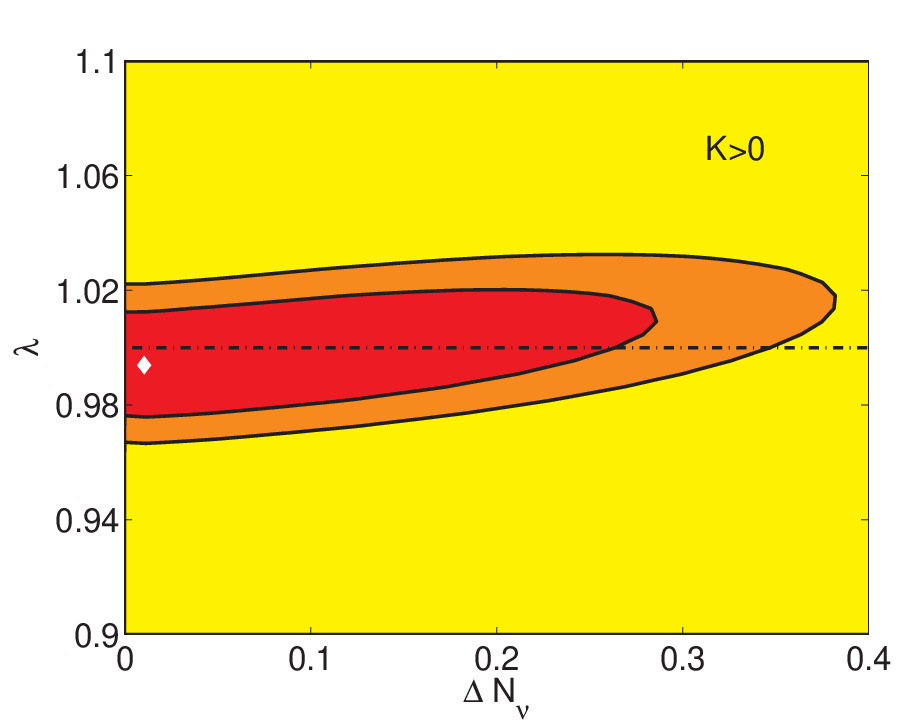
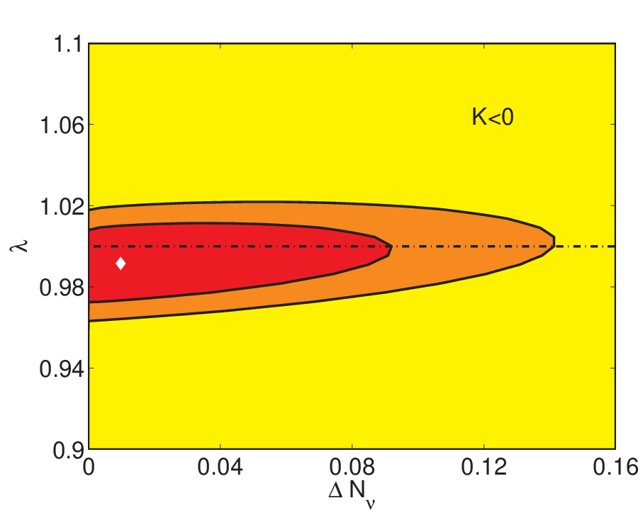
In summary, the scenario at hand involves seven model parameters namely the cosmological parameters $\Omega_{m0}$, $\Omega_{b0}$, $\Omega_{k0}$, $\Omega_{r0}$ and $H_{0}$ and the model parameters $\lambda$, $\omega$ and $\Delta N_{\nu}$, subject to constraint equations (32) and (33). We marginalize over the cosmological parameters $\Omega_{m0}$, $\Omega_{b0}$, $\Omega_{r0}$ and $H_{0}$. Of the four remaining parameters, only two are independent. We choose $\lambda$ and $\Delta N_{\nu}$ as our free parameters. Once these are chosen, and for a given choice of curvature, $\Omega_{K0}$ and $\omega$ are immediately fixed from the constraint equations. In particular, $\omega$ can be determined by eliminating $\Omega_{K0}$ from relations (32) and (33):

This fractional-order equation in $\omega$ can have one or two roots. In the latter case we use the larger one, since our goal is to set an upper limit on $\omega$ (and hence on $\Lambda$). $\Omega_{K0}$ can then be found from $\omega$ using (33).

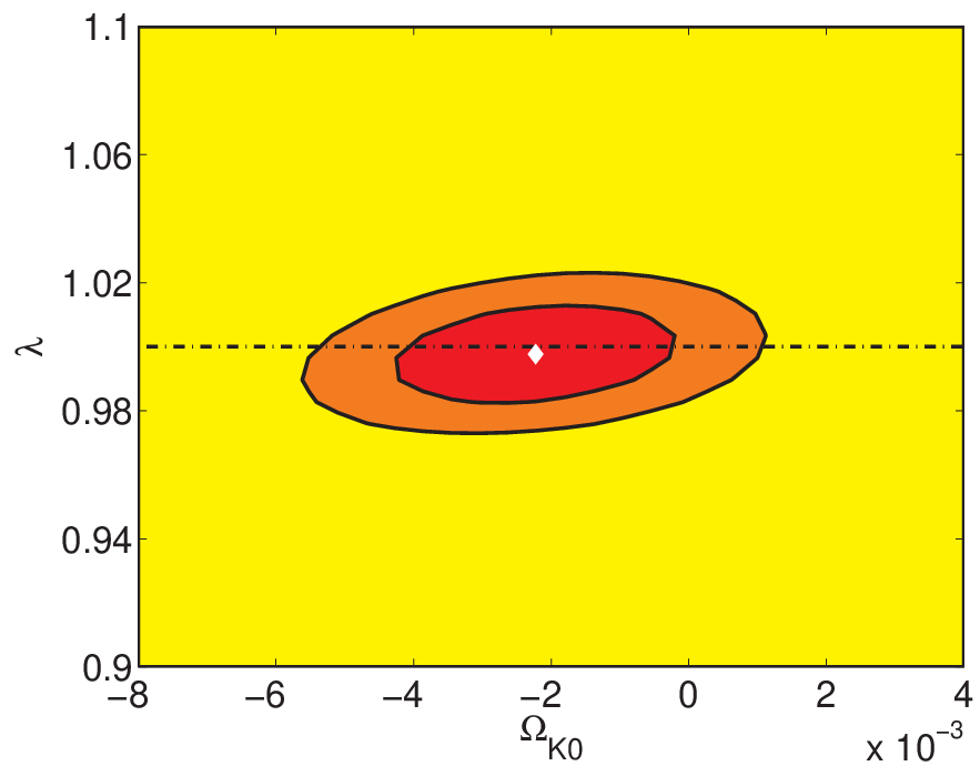
In Fig. 1 we display the likelihood-contours for the free parameters $\lambda$ vs $\Delta N_{\nu}$ for both positive and negative curvature. All other parameters have been marginalized over. The details and the techniques of the fitting procedure can be found in the Appendix of [109]. Additionally, in Table 1 we summarize the $1\sigma$ limits on the parameter values for the detailed-balance scenario. These bounds are in agreement with the corresponding ones of our previous work [109]. Furthermore, as we observe, the data constrain $\lambda$ to roughly $\lambda=1^{+0.01}_{-0.02}$ at the $1\sigma$ level, while its best fit value is very close to $1$ ($\lambda_{b.f}=0.006$) for both positive and negative curvature.

In units where $8\pi G_{\rm grav}=1$ relation (24) gives

Using this value and following the procedure of the previous subsection, the Friedmann equation (18) can be written as

where we have introduced the dimensionless parameters $\omega_{1}$, $\omega_{3}$ and $\omega_{4}$, related to the model parameters $\sigma_{1}$, $\sigma_{3}$ and $\sigma_{4}$ through:

Additionally, we consider the combination $\omega_{4}$ to be positive, in order to ensure that the Hubble parameter is real for all redshifts. $\omega_{4}>0$ is required also for the stability of the gravitational perturbations of the theory [13, 15]. For convenience we moreover assume $\sigma_{3}\geq 0$, that is $\omega_{3}\geq 0$.

In summary, the present scenario involves the following parameters: the cosmological parameters $H_{0}$, $\Omega_{m0}$, $\Omega_{K0}$, $\Omega_{b0}$, $\Omega_{r0}$, and the model parameters $\lambda$, $\omega_{1}$, $\omega_{3}$ and $\omega_{4}$. Similarly to the detailed-balance section these are subject to two constraints. The first one arises from the Friedman equation at $z=0$, which leads to

This constraint eliminates the parameter $w_{1}$. The second constraint arises from BBN considerations. The term involving $\omega_{3}$ represents the usual dark-radiation component. In addition, the $\omega_{4}$-term represents a kination-like component (a quintessence field dominated by kinetic energy [135, 136]). If $\Delta N_{\nu}$ represents the BBN upper limit on the total energy density of the universe beyond standard model constituents, then as we show in the Appendix of [109] we acquire the following constraint at the time of BBN ($z=z_{\rm BBN}$) [111, 112, 113, 114]:

It is clear that BBN imposes an extremely strong constraint on $\omega_{4}$, since its largest possible value (corresponding to $\omega_{3}=0$) is $\sim 10^{-24}$. Finally, $\omega_{3\text{max}}$ denotes the upper limit on $\omega_{3}$. In the following, we use expression (39) to eliminate $\omega_{4}$. For convenience, instead of $\omega_{3}$ we define a new parameter

which has the interesting physical meaning of denoting the ratio of the energy density of the Hořava-Lifshitz dark radiation to the total energy density of Hořava-Lifshitz dark radiation and kination-like components at the time of BBN.

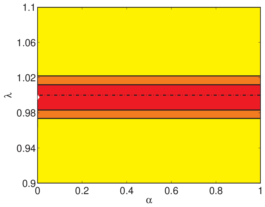
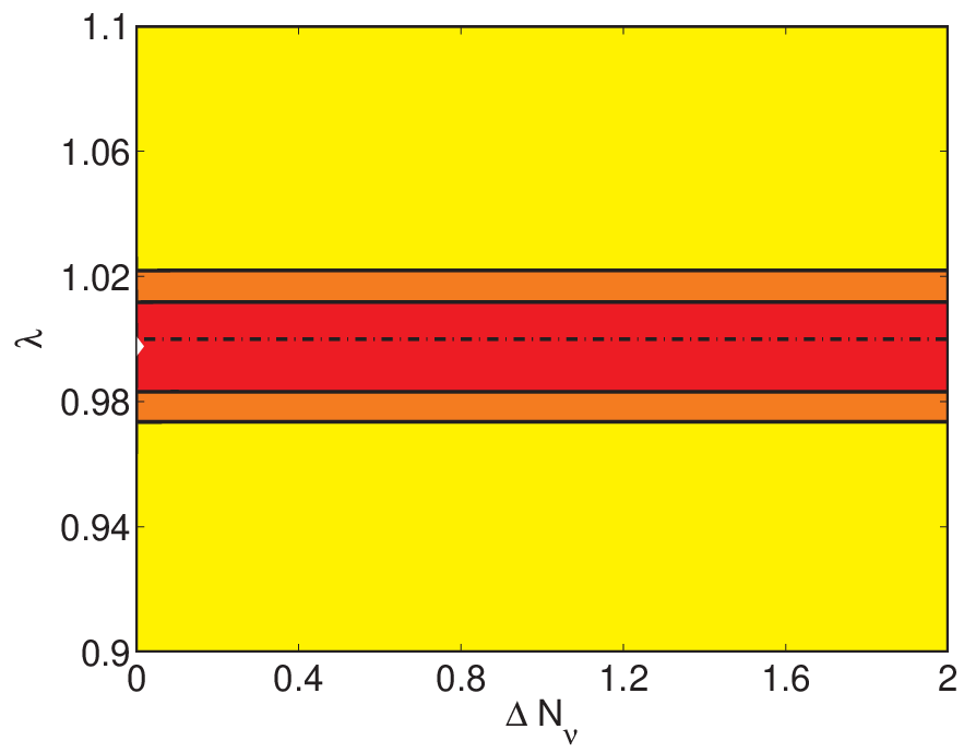
We use relation (39) to eliminate $\omega_{4}$ in favor of $\alpha$ and $\Delta N_{\nu}$, and treat $\lambda$, $\alpha$, $\Omega_{K0}$ and $\Delta N_{\nu}$ as our free parameters, marginalizing over $H_{0}$, $\Omega_{m0}$, $\Omega_{b0}$ and $\Omega_{r0}$. Using the combined SNIa+CMB+BAO data, we construct likelihood contours for different combinations of the above parameters, which are presented in Fig. 2. In each case, the free parameters not included in the plot have been marginalized over. The details and the techniques of the construction have been described in the Appendix of [109], with the only difference being that in the present work WMAP 7-year data [133] and the more recent Constitution Supernovae dataset [134] have been used. In Table 2 we summarize the $1\sigma$ limits on the parameter values for the beyond-detailed-balance scenario.

Furthermore, as we observe, in $1\sigma$ confidence the running parameter $\lambda$ of Hořava-Lifshitz gravity is restricted to the interval $|\lambda-1|\lesssim 0.02$, for the entire allowed range of $\omega_{3}$ (that is of $\sigma_{3}$). Finally, the best fit value for $\lambda$ restricts $|\lambda-1|$ to much more smaller values, namely $|\lambda_{b.f}-1|\approx 0.002$.

References

- [1] P. Horava, arXiv:0811.2217 [hep-th].
- [2] P. Horava, JHEP 0903, 020 (2009) [arXiv:0812.4287 [hep-th]].
- [3] P. Horava, Phys. Rev. D 79, 084008 (2009) [arXiv:0901.3775 [hep-th]].
- [4] P. Hořava, arXiv:0902.3657 [hep-th].
- [5] G. E. Volovik, arXiv:0904.4113 [gr-qc].
- [6] R. G. Cai, Y. Liu and Y. W. Sun, arXiv:0904.4104 [hep-th].
- [7] R. G. Cai, B. Hu and H. B. Zhang, arXiv:0905.0255 [hep-th].
- [8] D. Orlando and S. Reffert, arXiv:0905.0301 [hep-th].
- [9] T. Nishioka, arXiv:0905.0473 [hep-th].
- [10] R. A. Konoplya, arXiv:0905.1523 [hep-th].
- [11] C. Charmousis, G. Niz, A. Padilla and P. M. Saffin, arXiv:0905.2579 [hep-th].
- [12] T. P. Sotiriou, M. Visser and S. Weinfurtner, Phys. Rev. Lett. 102, 251601 (2009) [arXiv:0904.4464 [hep-th]].
- [13] T. P. Sotiriou, M. Visser and S. Weinfurtner, JHEP 0910, 033 (2009) [arXiv:0905.2798 [hep-th]].
- [14] C. Germani, A. Kehagias and K. Sfetsos, JHEP 0909, 060 (2009) [arXiv:0906.1201 [hep-th]].
- [15] C. Bogdanos and E. N. Saridakis, arXiv:0907.1636 [hep-th].
- [16] J. Kluson, arXiv:0907.3566 [hep-th].
- [17] N. Afshordi, arXiv:0907.5201 [hep-th].
- [18] Y. S. Myung, arXiv:0907.5256 [hep-th].
- [19] J. Alexandre, K. Farakos, P. Pasipoularides and A. Tsapalis, arXiv:0909.3719 [hep-th].
- [20] D. Blas, O. Pujolas and S. Sibiryakov, arXiv:0909.3525 [hep-th].
- [21] D. Capasso and A. P. Polychronakos, arXiv:0909.5405 [hep-th].
- [22] B. Chen, S. Pi and J. Z. Tang, arXiv:0910.0338 [hep-th].
- [23] S. Nojiri and S. D. Odintsov, arXiv:0905.4213 [hep-th].
- [24] J. Kluson, arXiv:0910.5852 [hep-th].
- [25] J. Kluson, arXiv:1002.2849 [hep-th].
- [26] M. Li and Y. Pang, arXiv:0905.2751 [hep-th].
- [27] M. Visser, arXiv:0902.0590 [hep-th].
- [28] J. Chen and Y. Wang, arXiv:0905.2786 [gr-qc].
- [29] B. Chen and Q. G. Huang, arXiv:0904.4565 [hep-th].
- [30] F. W. Shu and Y. S. Wu, arXiv:0906.1645 [hep-th].
- [31] G. Calcagni, arXiv:0904.0829 [hep-th].
- [32] E. Kiritsis and G. Kofinas, arXiv:0904.1334 [hep-th].
- [33] H. Lu, J. Mei and C. N. Pope, arXiv:0904.1595 [hep-th].
- [34] H. Nastase, arXiv:0904.3604 [hep-th].
- [35] E. O. Colgain and H. Yavartanoo, arXiv:0904.4357 [hep-th].
- [36] A. Ghodsi, arXiv:0905.0836 [hep-th].
- [37] M. Minamitsuji, arXiv:0905.3892 [astro-ph.CO].
- [38] A. Ghodsi and E. Hatefi, arXiv:0906.1237 [hep-th].
- [39] P. Wu and H. W. Yu, arXiv:0909.2821 [gr-qc].
- [40] I. Cho and G. Kang, arXiv:0909.3065 [hep-th].
- [41] C. G. Boehmer and F. S. N. Lobo, arXiv:0909.3986 [gr-qc].
- [42] D. Momeni, arXiv:0910.0594 [gr-qc].
- [43] M. R. Setare and D. Momeni, arXiv:0911.1877 [hep-th].
- [44] E. Kiritsis, arXiv:0911.3164 [hep-th].
- [45] R. G. Cai and A. Wang, arXiv:1001.0155 [hep-th].
- [46] M. Chaichian, S. Nojiri, S. D. Odintsov, M. Oksanen and A. Tureanu, arXiv:1001.4102 [hep-th].
- [47] A. Ali, S. Dutta, E. N. Saridakis and A. A. Sen, arXiv:1004.2474 [astro-ph.CO].
- [48] S. Carloni, E. Elizalde and P. J. Silva, arXiv:0909.2219 [hep-th].
- [49] G. Leon and E. N. Saridakis, JCAP 0911, 006 (2009) [arXiv:0909.3571 [hep-th]].
- [50] Y. S. Myung, Y. W. Kim, W. S. Son and Y. J. Park, arXiv:0911.2525 [gr-qc].
- [51] I. Bakas, F. Bourliot, D. Lust and M. Petropoulos, Class. Quant. Grav. 27, 045013 (2010) [arXiv:0911.2665 [hep-th]].
- [52] Y. S. Myung, Y. W. Kim, W. S. Son and Y. J. Park, arXiv:1001.3921 [gr-qc].
- [53] S. Mukohyama, K. Nakayama, F. Takahashi and S. Yokoyama, arXiv:0905.0055 [hep-th].
- [54] T. Takahashi and J. Soda, arXiv:0904.0554 [hep-th].
- [55] S. Koh, arXiv:0907.0850 [hep-th].
- [56] M. i. Park, arXiv:0910.1917 [hep-th].
- [57] M. i. Park, arXiv:0910.5117 [hep-th].
- [58] Y. S. Myung, arXiv:0911.0724 [hep-th].
- [59] S. Mukohyama, arXiv:0904.2190 [hep-th].
- [60] Y. S. Piao, arXiv:0904.4117 [hep-th].
- [61] X. Gao, arXiv:0904.4187 [hep-th].
- [62] B. Chen, S. Pi and J. Z. Tang, arXiv:0905.2300 [hep-th].
- [63] X. Gao, Y. Wang, R. Brandenberger and A. Riotto, arXiv:0905.3821 [hep-th].
- [64] Y. F. Cai and X. Zhang, Phys. Rev. D 80, 043520 (2009) [arXiv:0906.3341 [astro-ph.CO]].
- [65] A. Wang and R. Maartens, arXiv:0907.1748 [hep-th].
- [66] T. Kobayashi, Y. Urakawa and M. Yamaguchi, arXiv:0908.1005 [astro-ph.CO].
- [67] A. Wang, D. Wands and R. Maartens, arXiv:0909.5167 [hep-th].
- [68] T. Kobayashi, Y. Urakawa and M. Yamaguchi, arXiv:1002.3101 [hep-th].
- [69] R. Brandenberger, arXiv:0904.2835 [hep-th].
- [70] R. H. Brandenberger, arXiv:0905.1514 [hep-th].
- [71] Y. F. Cai and E. N. Saridakis, JCAP 0910, 020 (2009) [arXiv:0906.1789 [hep-th]].
- [72] T. Suyama, arXiv:0909.4833 [hep-th].
- [73] E. Czuchry, arXiv:0911.3891 [hep-th].
- [74] X. Gao, Y. Wang, W. Xue and R. Brandenberger, arXiv:0911.3196 [hep-th].
- [75] U. H. Danielsson and L. Thorlacius, JHEP 0903, 070 (2009) [arXiv:0812.5088 [hep-th]].
- [76] R. G. Cai, L. M. Cao and N. Ohta, arXiv:0904.3670 [hep-th].
- [77] Y. S. Myung and Y. W. Kim, arXiv:0905.0179 [hep-th].
- [78] A. Kehagias and K. Sfetsos, Phys. Lett. B 678, 123 (2009) [arXiv:0905.0477 [hep-th]].
- [79] R. B. Mann, arXiv:0905.1136 [hep-th].
- [80] G. Bertoldi, B. A. Burrington and A. Peet, arXiv:0905.3183 [hep-th].
- [81] M. i. Park, JHEP 0909, 123 (2009) [arXiv:0905.4480 [hep-th]].
- [82] A. Castillo and A. Larranaga, arXiv:0906.4380 [gr-qc].
- [83] M. Botta-Cantcheff, N. Grandi and M. Sturla, arXiv:0906.0582 [hep-th].
- [84] H. W. Lee, Y. W. Kim and Y. S. Myung, arXiv:0907.3568 [hep-th].
- [85] N. Varghese and V. C. Kuriakose, arXiv:0909.4944 [gr-qc].
- [86] E. Kiritsis and G. Kofinas, JHEP 1001, 122 (2010) [arXiv:0910.5487 [hep-th]].
- [87] B. R. Majhi, Phys. Lett. B 686, 49 (2010) [arXiv:0911.3239 [hep-th]].
- [88] J. Greenwald, A. Papazoglou and A. Wang, arXiv:0912.0011 [hep-th].
- [89] F. S. N. Lobo, T. Harko and Z. Kovacs, arXiv:1001.3517 [gr-qc].
- [90] E. N. Saridakis, arXiv:0905.3532 [hep-th].
- [91] M. i. Park, arXiv:0906.4275 [hep-th].
- [92] C. Appignani, R. Casadio and S. Shankaranarayanan, arXiv:0907.3121 [hep-th].
- [93] M. R. Setare, arXiv:0909.0456 [hep-th].
- [94] R. Garattini, arXiv:0912.0136 [gr-qc].
- [95] M. Jamil and E. N. Saridakis, arXiv:1003.5637 [physics.gen-ph].
- [96] S. S. Kim, T. Kim and Y. Kim, arXiv:0907.3093 [hep-th].
- [97] L. Iorio and M. L. Ruggiero, arXiv:0909.2562 [gr-qc].
- [98] L. Iorio and M. L. Ruggiero, arXiv:0909.5355 [gr-qc].
- [99] K. Izumi and S. Mukohyama, arXiv:0911.1814 [hep-th].
- [100] T. Harko, Z. Kovacs and F. S. N. Lobo, arXiv:0908.2874 [gr-qc].
- [101] A. Wang and Y. Wu, arXiv:0905.4117 [hep-th].
- [102] R. G. Cai, L. M. Cao and N. Ohta, arXiv:0905.0751 [hep-th].
- [103] R. G. Cai and N. Ohta, arXiv:0910.2307 [hep-th].
- [104] D. Blas, O. Pujolas and S. Sibiryakov, JHEP 0910, 029 (2009) [arXiv:0906.3046 [hep-th]].
- [105] K. Koyama and F. Arroja, arXiv:0910.1998 [hep-th].
- [106] A. Papazoglou and T. P. Sotiriou, arXiv:0911.1299 [hep-th].
- [107] M. Henneaux, A. Kleinschmidt and G. L. Gomez, Phys. Rev. D 81, 064002 (2010) [arXiv:0912.0399 [hep-th]].
- [108] J. O. Gong, S. Koh and M. Sasaki, arXiv:1002.1429 [hep-th].
- [109] S. Dutta and E. N. Saridakis, JCAP 1001, 013 (2010) [arXiv:0911.1435 [hep-th]].
- [110] S. M. Carroll and E. A. Lim, Phys. Rev. D 70, 123525 (2004) [arXiv:hep-th/0407149].
- [111] K. Hagiwara et al. [Particle Data Group], Phys. Rev. D 66, 010001 (2002).
- [112] K. A. Olive, G. Steigman and T. P. Walker, Phys. Rept. 333, 389 (2000) [arXiv:astro-ph/9905320].
- [113] G. Steigman, Int. J. Mod. Phys. E 15, 1 (2006) [arXiv:astro-ph/0511534].
- [114] R. A. Malaney and G. J. Mathews, Phys. Rept. 229, 145 (1993).
- [115] E. Komatsu et al. [WMAP Collaboration], Astrophys. J. Suppl. 180, 330 (2009) [arXiv:0803.0547 [astro-ph]].
- [116] A. R. Liddle and R. J. Scherrer, Phys. Rev. D 59, 023509 (1999) [arXiv:astro-ph/9809272].
- [117] R. Dave, R. R. Caldwell and P. J. Steinhardt, Phys. Rev. D 66, 023516 (2002) [arXiv:astro-ph/0206372].
- [118] D. C. Dai, S. Dutta and D. Stojkovic, Phys. Rev. D 80, 063522 (2009) [arXiv:0909.0024 [astro-ph.CO]].
- [119] T. Chiba, S. Dutta and R. J. Scherrer, Phys. Rev. D 80, 043517 (2009) [arXiv:0906.0628 [astro-ph.CO]].
- [120] S. Dutta, E. N. Saridakis and R. J. Scherrer, Phys. Rev. D 79, 103005 (2009) [arXiv:0903.3412 [astro-ph.CO]].
- [121] S. Dutta and R. J. Scherrer, Phys. Lett. B 676, 12 (2009) [arXiv:0902.1004 [astro-ph.CO]].
- [122] S. Dutta and R. J. Scherrer, Phys. Rev. D 78, 123525 (2008) [arXiv:0809.4441 [astro-ph]].
- [123] S. Dutta and R. J. Scherrer, Phys. Rev. D 78, 083512 (2008) [arXiv:0805.0763 [astro-ph]].
- [124] J. L. Crooks, J. O. Dunn, P. H. Frampton, H. R. Norton and T. Takahashi, Astropart. Phys. 20, 361 (2003) [arXiv:astro-ph/0305495].
- [125] K. Ichikawa and T. Takahashi, Phys. Rev. D 73, 083526 (2006) [arXiv:astro-ph/0511821].
- [126] G. Barenboim, E. Fernandez-Martinez, O. Mena and L. Verde, arXiv:0910.0252 [astro-ph.CO].
- [127] Y. Wang and P. Mukherjee, Phys. Rev. D 76, 103533 (2007) [arXiv:astro-ph/0703780].
- [128] E. L. Wright, Astrophys. J. 664, 633 (2007) [arXiv:astro-ph/0701584].
- [129] K. Ichikawa, M. Kawasaki, T. Sekiguchi and T. Takahashi, JCAP 0612, 005 (2006) [arXiv:astro-ph/0605481].
- [130] K. Ichikawa and T. Takahashi, JCAP 0702, 001 (2007) [arXiv:astro-ph/0612739].
- [131] C. Clarkson, M. Cortes and B. A. Bassett, JCAP 0708, 011 (2007) [arXiv:astro-ph/0702670].
- [132] J. M. Virey, D. Talon-Esmieu, A. Ealet, P. Taxil and A. Tilquin, JCAP 0812, 008 (2008) [arXiv:0802.4407 [astro-ph]].
- [133] E. Komatsu et al., arXiv:1001.4538 [astro-ph.CO].
- [134] M. Hicken et al., Astrophys. J. 700, 1097 (2009) [arXiv:0901.4804 [astro-ph.CO]].
- [135] M. Joyce, Phys. Rev. D 55, 1875 (1997) [arXiv:hep-ph/9606223].
- [136] M. Joyce and T. Prokopec, Phys. Rev. D 57, 6022 (1998) [arXiv:hep-ph/9709320].
- [137] D. Blas, O. Pujolas and S. Sibiryakov, arXiv:0912.0550 [hep-th].
- [138] L. I. Schiff, Proc. Nat. Acad. Sci. 46, 871 (1960).
- [139] K. Nordtvedt, Phys. Rev. 169, 1017 (1968).
- [140] C. M. Will, Astrophys. J. 163, 611 (1971).
- [141] C. M. Will, Theory and experiment in gravitational physics, Cambridge University Press, Cambridge, UK (1993).