跳到论文正文
W Papers独立论文阅读器 arXiv:1002.3330 论文正文 计算阅读时间 · 0%
引用这篇论文根据当前论文元数据生成,正式投稿前建议核对。


License: arXiv.org perpetual non-exclusive license
arXiv:1002.3330v2 [cs.LO] 18 Feb 2010

Deriving Relationship Between Semantic Models - An Approach for cCSP

Shamim H. Ripon , Michael Butler ††thanks: S. Ripon is the corresponding author Affiliation:  Department of Computing Science, University of Glasgow, UK Affiliation:  School of Electronics and Computer Science, University of Southampton, UK
Abstract

Formal semantics offers a complete and rigorous definition of a language. It is important to define different semantic models for a language and different models serve different purposes. Building equivalence between different semantic models of a language strengthen its formal foundation. This paper shows the derivation of denotational semantics from operational semantics of the language cCSP. The aim is to show the correspondence between operational and trace semantics. We extract traces from operational rules and use induction over traces to show the correspondence between the two semantics of cCSP.

Index Terms:
Compensating CSP, semantic relationship, trace semantics, operational semantics.

I Introduction

A formal semantics offers a complete, and rigorous definition of a language. Operational and denotational semantics are two well-known methods of assigning meaning to programming languages and both semantics are necessary for a complete description of the language. Denotational semantics associates an element of a semantic domain to each expression in the language and the semantic is compositional. Traces are one of the ways to define denotational semantics. A trace gives the global picture of the behaviour. The common way of defining operational semantics is to provide state transition systems for the language, where the transition system models the computation steps of expressions in the language and allows the formal analysis of the language.

Compensating CSP (cSCP) [1] is a language defined to model long running business transactions within the framework of Hoare’s CSP [2] process algebra. Business transactions need to deal with faults that can arise at any stage of the transactions. Compensation is defined in [3] as an action taken to recover from error in business transactions or cope with a change of plan. cCSP provides constructs for orchestration of compensations to model business transactions. With the introduction of the language, both traces [1] and operational [4] semantics have been defined. Both semantics have valuable non-overlapping application and we want to use them both. The key question is ”How they are related?”.

This paper draws the correspondence of two different semantic representation of a language which strengthen the formal foundation of the language. In particular, the aim is to accomplish the unification between operational and denotational approach of cCSP. The unification is based on the approach where we use the transition rules from operational semantics to derive the traces and then show that these derived traces correspond to the original traces by using induction over the derived traces. Completing the derivation means that any of the presentations can be accepted as a primary definition of the meaning of the language and each of the definitions can even safely and consistently be used at different times and for different purposes.

The reset of the paper is organised as follows. A brief overview of cCSP along with an example is given in Section II. The trace and the operational semantics of cCSP are outlined in Section III. We describe the how we define and prove a relationship between the semantic models in Section IV. We define theorems and supporting lemmas to establish the relationship for both standard and compensable processes. We outline some lessons from the experiment and then summarise some related work in Section V and Section VI respectively. We draw our conclusion in Section VII.

II Compensating CSP

The introduction of the cCSP language was inspired by two ideas: transaction processing features, and process algebra. Like standard CSP, processes in cCSP are modelled in terms of the atomic events they can engage in. The language provides operators that support sequencing, choice, parallel composition of processes. In order to support failed transaction, compensation operators are introduced. The processes are categorised into standard, and compensable processes. A standard process does not have any compensation, but compensation is part of a compensable process that is used to compensate a failed transaction. We use notations, such as, P,Q,..P,Q,.. to identify standard processes, and PP,QQ,..PP,QQ,.. to identify compensable processes. A subset of the original cCSP is considered in this paper, which includes most of the operators, is summarised in Fig. 1.

Refer to caption

Fig. 1: cCSP syntax

The basic unit of the standard processes is an atomic event (AA). The other operators are the sequential (P​ ; ​QP\mbox{\penalty\ ;\penalty\ }Q), and the parallel composition (P∥QP\mathrel{\mathord{\parallel}}Q), the choice operator (P2QP\mathrel{\mathord{\Box}}Q), the interrupt handler (P�QP\rhd Q), the empty process SKIPSKIP, raising an interrupt THROWTHROW, and yielding to an interrupt YIELDYIELD. A process that is ready to terminate is also willing to yield to an interrupt. In a parallel composition, throwing an interrupt by one process synchronises with yielding in another process. Yield points are inserted in a process through YIELDYIELD. For example, (P​ ; ​YIELD​ ; ​QP\mbox{\penalty\ ;\penalty\ }YIELD\mbox{\penalty\ ;\penalty\ }Q) is willing to yield to an interrupt in between the execution of PP, and QQ. The basic way of constructing a compensable process is through a compensation pair (P÷QP\div Q), which is constructed from two standard processes, where PP is called the forward behaviour that executes during normal execution, and QQ is called the associated compensation that is designed to compensate the effect of PP when needed. The sequential composition of compensable processes is defined in such a way that the compensations of the completed tasks will be accumulated in reverse to the order of their original composition, whereas compensations from the compensable parallel processes will be placed in parallel. In this paper, we define only the asynchronous composition of processes, where processes interleave with each other during normal execution, and synchronise during termination. By enclosing a compensable process PPPP inside a transaction block [PP][\,PP\,], we get a complete transaction and the transaction block itself is a standard process. Successful completion of PPPP represents successful completion of the block. But, when the forward behaviour of PPPP throws an interrupt, the compensations are executed inside the block, and the interrupt is not observable from outside of the block. SKIPP,THROWWSKIPP,THROWW, and YIELDDYIELDD are the compensable counterpart of the corresponding standard processes and they are defined as follows:

S​K​I​P​P\displaystyle SKIPP =\displaystyle= S​K​I​P÷S​K​I​P,\displaystyle SKIP\div SKIP,
Y​I​E​L​D​D\displaystyle YIELDD =\displaystyle= Y​I​E​L​D÷S​K​I​P\displaystyle YIELD\div SKIP
T​H​R​O​W​W\displaystyle THROWW =\displaystyle= T​H​R​O​W÷S​K​I​P\displaystyle THROW\div SKIP

To illustrate the use of cCSP, we present an example of a transaction for processing customer orders in a warehouse in Fig.2. The first step in the transaction is a compensation pair. The primary action of this pair is to accept the order and deduct the order quantity from the inventory database. The compensation action simply adds the order quantity back to the total in the inventory database. After an order is received from a customer, the order is packed for shipment, and a courier is booked to deliver the goods to the customer. The PackOrder process packs each of the items in the order in parallel. Each 𝑃𝑎𝑐𝑘𝐼𝑡𝑒𝑚\mathit{PackItem} activity can be compensated by a corresponding 𝑈𝑛𝑝𝑎𝑐𝑘𝐼𝑡𝑒𝑚\mathit{UnpackItem}. Simultaneously with the packing of the order, a credit check is performed on the customer. The credit check is performed in parallel because it normally succeeds, and in this normal case the company does not wish to delay the order unnecessarily. In the case that a credit check fails, an interrupt is thrown causing the transaction to stop its execution, with the courier possibly having been booked and possibly some of the items having being packed. In case of failure, the semantics of the transaction block will ensure that the appropriate compensation activities will be invoked for those activities that already did take place.
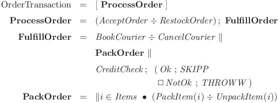
Refer to caption
Fig. 2: Warehouse order processing

III Semantic Models

This section briefly outlines the trace and the operational semantics of cCSP.

III-A Trace Semantics

A trace of a process records the history of behaviour up to some point. We show the operators on traces which are then lifted to operators on set of traces. Traces considered for cCSP are non-empty sets.

The trace of a standard process is of the form s​⟨ω⟩s\langle\omega\rangle where s∈Σ∗s\in\Sigma^{*} (Σ\Sigma is alphabet of normal events) and ω∈Ω\omega\in\Omega (Ω={X,!,?}\Omega=\{\tick,\,!,\,?\}), which means all traces end with any of the events in Ω\Omega, which is called a terminal event. The terminal events represent the termination of a process. Successful termination is shown by a X\tick. Termination by either throwing or yielding an interrupt is shown by !! or ?? respectively. In sequential composition (p​ ; ​q)(p\mbox{\penalty\ ;\penalty\ }q), the concatenated observable traces pp and qq, only when pp terminates successfully,(ends with X\tick), otherwise the trace is only pp. The traces of two parallel processes are p​⟨ω⟩|q​⟨ω′⟩p\langle\omega\rangle\|q\langle\omega^{\prime}\rangle which corresponds to the set (p∣​∣​∣qp\mathrel{\mathord{\mid}\mathord{\mid}\mathord{\mid}}q), the possible interleaving of traces of both processes and followed by ω&ω′\omega\&\omega^{\prime}, the synchronisation of ω\omega and ω′\omega^{\prime}. The trace semantics of standard processes are shown in Fig. 3.

Refer to caption

Fig. 3: Trace semantics of standard processes

Compensable processes are comprised of forward and compensation behaviour. The traces of compensable processes are of pair of traces of the form (s⁡⟨ω⟩,s′​⟨ω′⟩)(s\langle\omega\rangle,s^{\prime}\langle\omega^{\prime}\rangle), where s​⟨ω⟩s\langle\omega\rangle is the forward behaviour and s′​⟨ω′⟩s^{\prime}\langle\omega^{\prime}\rangle is the compensation behaviour. In sequential composition, the forward traces correspond to the original forward behaviour and followed by the traces of the compensation. Traces of parallel composition are defined as the interleaving of forward traced and then follows the interleaving of compensation. The traces of a compensation pair are the traces of both of the processes of the pair when the forward process (PP) terminate with a ⟨X⟩\langle\tick\rangle, otherwise the traces of the pair are the traces of the forward process followed by only a ⟨X⟩\langle\tick\rangle. The traces of a transaction block are only the traces of compensable processes inside the block when the process terminates with a ⟨X⟩\langle\tick\rangle, otherwise when the forward process inside the block terminates with a ⟨!⟩\langle!\rangle the traces of the block are the traces of the forward process followed by the traces of the compensation. Fig. 4 outlines the traces of compensable processes.

Refer to caption

Fig. 4: Trace semantics of compensable processes

The following healthiness conditions declare that processes consist of some terminating or interrupting behaviour which ensures that the traces of processes are non-empty:

  • •

    p​⟨X⟩∈T⁡(P)p\langle\tick\rangle\in T(P) or p⟨!⟩∈T(P)p\langle\,!\,\rangle\in T(P), for some pp

  • •

    (p⁡⟨X⟩,p′)∈T⁡(PP)(p\langle\tick\rangle,p^{\prime})\in T(PP) or (p⟨!⟩,p′)∈T(PP),(p\langle\,!\,\rangle,p^{\prime})\in T(PP), for some p,p′p,p^{\prime}

III-B Operational Semantics

By using labelled transition systems [5], the operational semantics specifies the relation between states of a program. Two types of transitions are define to present the transition relation of process terms: normal and terminal. A normal transition is defined by a normal event (a∈Σa\in\Sigma) and a terminal transition is defined by a terminal event (ω∈Ω\omega\in\Omega) .

For a standard process, a normal transition makes the transition of a process term from one state to its another state (PP to P′P^{\prime}). The terminal transition, on the other hand terminates a standard process to a null process (0):

P⟶aP′,\displaystyle P\stackrel{{\scriptstyle a}}{{\longrightarrow}}P^{\prime}, P⟶ω0\displaystyle P\stackrel{{\scriptstyle\omega}}{{\longrightarrow}}0

In sequential composition (P​ ; ​QP\mbox{\penalty\ ;\penalty\ }Q), the process QQ can start only when the process PP terminates successfully (with X\tick). If PP terminates with !! or ?? the process QQ will not start. In parallel composition each process can evolve independently and processes synchronise only on terminal events. The transition rules for standard processes are outlined in Fig. 5.

Refer to caption

Fig. 5: Operational semantics of standard processes

For compensable processes, the normal transitions are same as standard processes. However, the terminal events terminate the forward behaviour of compensable processes, additionally, the compensation are stored for future reference.

P​P⟶aP​P′,\displaystyle PP\stackrel{{\scriptstyle a}}{{\longrightarrow}}PP^{\prime}, P​P⟶ωP(P is the compensation)\displaystyle PP\stackrel{{\scriptstyle\omega}}{{\longrightarrow}}P\quad\mbox{($P$ is the compensation)}

In sequential composition (PP​ ; ​QQPP\mbox{\penalty\ ;\penalty\ }QQ), when PPPP terminates, its compensation (PP) is stored and QQQQ starts to execute. In this scenario, we get an auxiliary construct (⟨QQ,P⟩\langle QQ,P\rangle) where the processes have no particular operational relation between them. After termination of the process QQQQ, its compensation (QQ) is accumulated in front of PP i.e., (Q​ ; ​PQ\mbox{\penalty\ ;\penalty\ }P). In the parallel composition, the main difference with the standard processes is that after termination of the forward behaviour the compensations are accumulated in parallel. The transition rules of compensable processes are summarised in Fig. 6.

Refer to caption

Fig. 6: Operational semantics of compensable processes

A non-terminal event changes the state of the process inside the block. Successful completion of the forward process inside the block means completion of the whole block, but throwing a interrupt by the compensable process inside the block results the compensation to run. In compensation pair, after successful completion of the forward behaviour the compensation will be stored for future use, however, unsuccessful termination, i.e, terminates by !! or ?? results an empty compensation (Fig. 5).

IV Relating Semantic Models

In this section we describe the steps to derive a relationship between the two semantic models of cCSP. We follow a systematic approach to derive the relationship where traces are first extracted from the transition rules and prove that the extracted traces correspond to the original trace definition. The steps of deriving the semantic relation are shown in Fig. 7.

Refer to caption
Fig. 7: Steps to derive relationship between semantic models

The operational semantics leads to lifted transition relations labelled by sequences of events. This is defined recursively. For a standard process PP,

P⟶⟨ω⟩Q\displaystyle P\stackrel{{\scriptstyle\langle\omega\rangle}}{{\longrightarrow}}Q =\displaystyle\penalty\ =\, P⟶ωQ\displaystyle P\stackrel{{\scriptstyle\omega}}{{\longrightarrow}}Q
P⟶⟨a⟩​tQ\displaystyle P\stackrel{{\scriptstyle\langle a\rangle t}}{{\longrightarrow}}Q =\displaystyle\penalty\ =\, ∃P′⋅P⟶aP′∧P′⟶tQ\displaystyle\mathop{\mathstrut{\exists}}\nolimits P^{\prime}\cdot P\stackrel{{\scriptstyle a}}{{\longrightarrow}}P^{\prime}\,\mathrel{\wedge}\,P^{\prime}\stackrel{{\scriptstyle t}}{{\longrightarrow}}Q

The derived traces of a standard process PP is defined as DT⁡(P)DT(P). Let t∈DT⁡(P)t\in DT(P), then we get the following definition,

t∈D​T​(P)\displaystyle t\in DT(P) =\displaystyle= P⟶t0\displaystyle P\stackrel{{\scriptstyle t}}{{\longrightarrow}}0 (1)

Compensable processes have both forward and compensation behaviour. A compensable process is defined as a pair of traces. Hence, it is required to extract traces from both forward and compensation behaviour. The forward behaviour of a compensable process PPPP is defined as follows:

P​P⟶tR(t ends with ω)\displaystyle PP\stackrel{{\scriptstyle t}}{{\longrightarrow}}R\quad(\mbox{$t$ ends with $\omega$})

where tt is the trace of the forward behaviour. RR is the attached compensation. The behaviour of compensation is similar to standard processes and by reusing that we get the following definition:

P​P⟶(t,t′)0\displaystyle PP\stackrel{{\scriptstyle(t,t^{\prime})}}{{\longrightarrow}}0 =\displaystyle\penalty\ =\, ∃R⋅P​P⟶tR∧R⟶t′0\displaystyle\mathop{\mathstrut{\exists}}\nolimits R\cdot PP\stackrel{{\scriptstyle t}}{{\longrightarrow}}R\,\mathrel{\wedge}\,R\stackrel{{\scriptstyle t^{\prime}}}{{\longrightarrow}}0

where t′t^{\prime} is the trace of the compensation. For a compensable process PPPP, the derived traces DT⁡(PP)DT(PP) is defined as follows:

(t,t′)∈D​T​(P​P)\displaystyle(t,t^{\prime})\in DT(PP) =\displaystyle\penalty\ =\, P​P⟶(t,t′)0\displaystyle PP\stackrel{{\scriptstyle(t,t^{\prime})}}{{\longrightarrow}}0

By using the definition of derived traces and the original traces we state the following theorem to define the relationship between the semantic models,

Theorem 1

For any standard process term PP, where P≠0P\neq 0

D​T​(P)=T⁡(P)\displaystyle DT(P)\,\,=\,\,T(P)

For any compensable process terms PPPP, where PP≠0PP\neq 0 and does not contain the term ⟨PP,P⟩\langle PP,P\rangle,

D​T​(P​P)\displaystyle DT(PP) =\displaystyle\penalty\ =\, T⁡(P​P)\displaystyle T(PP)

Traces are extracted for each term of the language, and its correspondence is shown with the corresponding traces in the trace semantics. Assume PP and QQ are standard process terms, then for all the operators, we prove that

t∈D​T​(P⊗Q)\displaystyle t\in DT(P\otimes Q) =\displaystyle\penalty\ \,=\,\, t∈T⁡(P⊗Q)\displaystyle t\in T(P\otimes Q) (2)

For each such operator ⊗\otimes, the proof is performed by induction over traces. In the proof we assume that, DT⁡(P)=T⁡(P)DT(P)\,=\,T(P) and DT⁡(Q)=T⁡(Q)DT(Q)\,=\,T(Q).

We follow similar style for compensable processes. Assuming DT⁡(PP)=T⁡(PP)DT(PP)\,=\,T(PP) and DT⁡(QQ)=T⁡(QQ)DT(QQ)\,=\,T(QQ) we show that,

(t,t′)∈D​T​(P​P⊗Q​Q)\displaystyle(t,t^{\prime})\in DT(PP\otimes QQ)\,\, =\displaystyle= (t,t′)∈T⁡(P​P⊗Q​Q)\displaystyle(t,t^{\prime})\in T(PP\otimes QQ) (3)

In the following sections we outline the proof steps showing the correspondence in (2) and (3) for both standard and compensable process terms.

IV-A Standard Processes

Sequential Composition: By using (2) the relationship between the semantic models is derived by showing that,

t∈DT⁡(P​ ; ​Q)=t∈T⁡(P​ ; ​Q)t\in DT(P\mbox{\penalty\ ;\penalty\ }Q)\,\,=\,\,t\in T(P\mbox{\penalty\ ;\penalty\ }Q)

From (1) we get the derived traces of the sequential composition,

t∈D​T​(P​ ; ​Q)\displaystyle t\in DT(P\mbox{\penalty\ ;\penalty\ }Q) =\displaystyle= (P​ ; ​Q)⟶t0\displaystyle(P\mbox{\penalty\ ;\penalty\ }Q)\stackrel{{\scriptstyle t}}{{\longrightarrow}}0

We also expand the definition of trace semantics as follows:

t\displaystyle t ∈T⁡(P​ ;​Q)\displaystyle\in\,T(P\mbox{\penalty\ \large{;}}\,Q)
=∃p,q⋅t=(p​ ; ​q)∧p∈T⁡(P)∧q∈T⁡(Q)\displaystyle=\,\mathop{\mathstrut{\exists}}\nolimits p,q\cdot t=(p\mbox{\penalty\ ;\penalty\ }q)\,\,\mathrel{\wedge}\,\,p\in T(P)\,\,\mathrel{\wedge}\,\,q\in T(Q)
=∃p,q⋅t=(p​ ; ​q)∧p∈D​T​(P)∧q∈D​T​(Q)\displaystyle=\,\mathop{\mathstrut{\exists}}\nolimits p,q\cdot t=(p\mbox{\penalty\ ;\penalty\ }q)\,\,\mathrel{\wedge}\,\,p\in DT(P)\,\,\mathrel{\wedge}\,\,q\in DT(Q)
=∃p,q⋅t=(p​ ; ​q)∧P⟶p0∧Q⟶q0\displaystyle=\,\mathop{\mathstrut{\exists}}\nolimits p,q\cdot t=(p\mbox{\penalty\ ;\penalty\ }q)\,\,\mathrel{\wedge}\,\,P\stackrel{{\scriptstyle p}}{{\longrightarrow}}0\,\,\mathrel{\wedge}\,\,Q\stackrel{{\scriptstyle q}}{{\longrightarrow}}0

Finally, from the above definitions of traces, the following lemma is formulated for the sequential composition of standard processes:

Lemma 1
(P​ ; ​Q)⟶t0=∃p,q⋅t=(p​ ; ​q)∧P⟶p0∧Q⟶q0\displaystyle(P\mbox{\penalty\ ;\penalty\ }Q)\stackrel{{\scriptstyle t}}{{\longrightarrow}}0\,=\,\mathop{\mathstrut{\exists}}\nolimits p,q\cdot t=(p\mbox{\penalty\ ;\penalty\ }q)\,\mathrel{\wedge}\,P\stackrel{{\scriptstyle p}}{{\longrightarrow}}0\,\mathrel{\wedge}\,Q\stackrel{{\scriptstyle q}}{{\longrightarrow}}0

The lemma is proved by applying induction over the trace tt, where t=⟨ω⟩t=\langle\omega\rangle is considered as the base case, and t=⟨a⟩​tt=\langle a\rangle t is considered as the inductive case. To support the proof of the lemma, two equations are derived from the transition rules. These derived equations are based on the event by which the transition rules are defined:

(P​ ; ​Q)⟶ω0\displaystyle(P\mbox{\penalty\ ;\penalty\ }Q)\stackrel{{\scriptstyle\omega}}{{\longrightarrow}}0 =\displaystyle\penalty\ =\, P⟶X0∧Q⟶ω0\displaystyle P\stackrel{{\scriptstyle\tick}}{{\longrightarrow}}0\,\mathrel{\wedge}\,Q\stackrel{{\scriptstyle\omega}}{{\longrightarrow}}0
∨\displaystyle\vee P⟶ω0∧ω≠X\displaystyle P\stackrel{{\scriptstyle\omega}}{{\longrightarrow}}0\,\mathrel{\wedge}\,\omega\neq\tick
(P​ ; ​Q)⟶aR\displaystyle(P\mbox{\penalty\ ;\penalty\ }Q)\stackrel{{\scriptstyle a}}{{\longrightarrow}}R =\displaystyle\penalty\ =\, ∃P′⋅P⟶aP′∧R=(P′​ ; ​Q)\displaystyle\mathop{\mathstrut{\exists}}\nolimits P^{\prime}\cdot P\stackrel{{\scriptstyle a}}{{\longrightarrow}}P^{\prime}\,\mathrel{\wedge}\,R=(P^{\prime}\mbox{\penalty\ ;\penalty\ }Q)
∨\displaystyle\vee P⟶X0∧Q⟶aR\displaystyle P\stackrel{{\scriptstyle\tick}}{{\longrightarrow}}0\,\mathrel{\wedge}\,Q\stackrel{{\scriptstyle a}}{{\longrightarrow}}R
Proof:


Basic step:  t=⟨ω⟩t=\langle\omega\rangle
(P​ ; ​Q)⟶⟨ω⟩0=(P​ ; ​Q)⟶ω0\begin{array}[]{rcl}(P\mbox{\penalty\ ;\penalty\ }Q)\stackrel{{\scriptstyle\langle\omega\rangle}}{{\longrightarrow}}0&=&(P\mbox{\penalty\ ;\penalty\ }Q)\stackrel{{\scriptstyle\omega}}{{\longrightarrow}}0\end{array}
“From transition rules sequential composition”

=\displaystyle= P⟶X0∧Q⟶ω0\displaystyle\penalty\ \,\,\,P\stackrel{{\scriptstyle\tick}}{{\longrightarrow}}0\,\,\wedge\,\,Q\stackrel{{\scriptstyle\omega}}{{\longrightarrow}}0 (4)
∨\displaystyle\vee P⟶ω0∧ω≠X\displaystyle\penalty\ P\stackrel{{\scriptstyle\omega}}{{\longrightarrow}}0\,\,\wedge\,\,\omega\neq\tick (5)

From (4)

P⟶X0∧Q⟶ω0\displaystyle P\stackrel{{\scriptstyle\tick}}{{\longrightarrow}}0\,\,\wedge\,\,Q\stackrel{{\scriptstyle\omega}}{{\longrightarrow}}0
=\displaystyle= ∃p,q⋅p=⟨X⟩∧q=⟨ω⟩∧⟨ω⟩=(p​ ; ​q)\displaystyle\mathop{\mathstrut{\exists}}\nolimits p,q\cdot\,p=\langle\tick\rangle\,\wedge\,q=\langle\omega\rangle\,\wedge\,\langle\omega\rangle=(p\mbox{\penalty\ ;\penalty\ }q)
∧\displaystyle\wedge P⟶p0∧Q⟶q0\displaystyle P\stackrel{{\scriptstyle p}}{{\longrightarrow}}0\,\wedge\,Q\stackrel{{\scriptstyle q}}{{\longrightarrow}}0
=\displaystyle= ∃p,q⋅⟨ω⟩=(p​ ; ​q)∧p=⟨X⟩\displaystyle\mathop{\mathstrut{\exists}}\nolimits p,q\cdot\langle\omega\rangle=(p\mbox{\penalty\ ;\penalty\ }q)\,\,\wedge\,\,p=\langle\tick\rangle
∧\displaystyle\wedge P⟶p0∧Q⟶q0\displaystyle\penalty\ P\stackrel{{\scriptstyle p}}{{\longrightarrow}}0\,\,\wedge\,\,Q\stackrel{{\scriptstyle q}}{{\longrightarrow}}0

From (5)

P⟶ω0∧ω≠X\displaystyle P\stackrel{{\scriptstyle\omega}}{{\longrightarrow}}0\,\,\wedge\,\,\omega\neq\tick
=\displaystyle= ∃p,q⋅p=⟨ω⟩∧ω≠X∧⟨ω⟩=(p​ ; ​q)\displaystyle\mathop{\mathstrut{\exists}}\nolimits p,q\cdot p=\langle\omega\rangle\,\,\wedge\,\,\omega\neq\tick\,\,\wedge\,\,\langle\omega\rangle=(p\mbox{\penalty\ ;\penalty\ }q)
∧\displaystyle\wedge P⟶p0∧Q⟶q0\displaystyle P\stackrel{{\scriptstyle p}}{{\longrightarrow}}0\,\,\wedge\,\,Q\stackrel{{\scriptstyle q}}{{\longrightarrow}}0
=\displaystyle= ∃p,q⋅⟨ω⟩=(p​ ; ​q)∧p≠⟨X⟩\displaystyle\mathop{\mathstrut{\exists}}\nolimits p,q\cdot\langle\omega\rangle=(p\mbox{\penalty\ ;\penalty\ }q)\,\,\wedge\,\,p\neq\langle\tick\rangle
∧\displaystyle\wedge P⟶p0∧Q⟶q0\displaystyle P\stackrel{{\scriptstyle p}}{{\longrightarrow}}0\,\,\wedge\,\,Q\stackrel{{\scriptstyle q}}{{\longrightarrow}}0

Therefore, for t=⟨ω⟩t=\langle\omega\rangle from (4) and (5)

∃p,q⋅⟨ω⟩=(p​ ; ​q)∧p=⟨X⟩\displaystyle\mathop{\mathstrut{\exists}}\nolimits p,q\cdot\langle\omega\rangle=(p\mbox{\penalty\ ;\penalty\ }q)\,\,\wedge\,\,p=\langle\tick\rangle
∧P⟶p0∧Q⟶q0\displaystyle\wedge\,P\stackrel{{\scriptstyle p}}{{\longrightarrow}}0\,\,\wedge\,\,Q\stackrel{{\scriptstyle q}}{{\longrightarrow}}0
∨\displaystyle\vee ∃p,q⋅⟨ω⟩=(p​ ; ​q)∧p≠⟨X⟩\displaystyle\mathop{\mathstrut{\exists}}\nolimits p,q\cdot\langle\omega\rangle=(p\mbox{\penalty\ ;\penalty\ }q)\,\,\wedge\,\,p\neq\langle\tick\rangle
∧P⟶p0∧Q⟶q0\displaystyle\wedge\,P\stackrel{{\scriptstyle p}}{{\longrightarrow}}0\,\,\wedge\,\,Q\stackrel{{\scriptstyle q}}{{\longrightarrow}}0
=\displaystyle= ∃p,q⋅⟨ω⟩=(p​ ; ​q)∧P⟶p0∧Q⟶q0\displaystyle\mathop{\mathstrut{\exists}}\nolimits p,q\cdot\langle\omega\rangle=(p\mbox{\penalty\ ;\penalty\ }q)\,\,\wedge\,\,P\stackrel{{\scriptstyle p}}{{\longrightarrow}}0\,\,\wedge\,\,Q\stackrel{{\scriptstyle q}}{{\longrightarrow}}0

Inductive step: t=⟨a⟩​tt=\langle a\rangle t
P​ ;​Q⟶⟨a⟩​t0=∃R⋅(P​ ; ​Q)⟶aR∧R⟶t0\begin{array}[]{rcl}P\mbox{\penalty\ \large{;}}\,Q\stackrel{{\scriptstyle\langle a\rangle t}}{{\longrightarrow}}0&=&\mathop{\mathstrut{\exists}}\nolimits R\cdot\,(P\mbox{\penalty\ ;\penalty\ }Q)\stackrel{{\scriptstyle a}}{{\longrightarrow}}R\,\,\wedge\,\,R\stackrel{{\scriptstyle t}}{{\longrightarrow}}0\end{array}

“From operational rules”

=\displaystyle= ∃P′⋅P⟶aP′∧(P′​ ; ​Q)⟶t0\displaystyle\penalty\ \,\,\,\mathop{\mathstrut{\exists}}\nolimits P^{\prime}\cdot\,P\stackrel{{\scriptstyle a}}{{\longrightarrow}}P^{\prime}\,\,\wedge\,\,(P^{\prime}\mbox{\penalty\ ;\penalty\ }Q)\stackrel{{\scriptstyle t}}{{\longrightarrow}}0 (6)
∨∃Q′⋅P⟶X0∧Q⟶aQ′∧Q′⟶t0\displaystyle\vee\,\mathop{\mathstrut{\exists}}\nolimits Q^{\prime}\cdot\,P\stackrel{{\scriptstyle\tick}}{{\longrightarrow}}0\,\,\wedge\,\,Q\stackrel{{\scriptstyle a}}{{\longrightarrow}}Q^{\prime}\,\,\wedge\,\,Q^{\prime}\stackrel{{\scriptstyle t}}{{\longrightarrow}}0 (7)

From (6)

∃P′⋅P⟶aP′∧(P′​ ; ​Q)⟶t0\displaystyle\mathop{\mathstrut{\exists}}\nolimits P^{\prime}\cdot\,P\stackrel{{\scriptstyle a}}{{\longrightarrow}}P^{\prime}\,\,\wedge\,\,(P^{\prime}\mbox{\penalty\ ;\penalty\ }Q)\stackrel{{\scriptstyle t}}{{\longrightarrow}}0
=\displaystyle= “Inductive hypothesis”
∃P′⋅P⟶aP′∧∃p′,q⋅t=(p′​ ; ​q)\displaystyle\mathop{\mathstrut{\exists}}\nolimits P^{\prime}\cdot\,P\stackrel{{\scriptstyle a}}{{\longrightarrow}}P^{\prime}\,\,\wedge\,\,\mathop{\mathstrut{\exists}}\nolimits p^{\prime},q\cdot\,t=(p^{\prime}\mbox{\penalty\ ;\penalty\ }q)
∧\displaystyle\wedge P′⟶p′0∧Q⟶q0\displaystyle P^{\prime}\stackrel{{\scriptstyle p^{\prime}}}{{\longrightarrow}}0\,\,\wedge\,\,Q\stackrel{{\scriptstyle q}}{{\longrightarrow}}0
=\displaystyle= “Combining existential quantifications”
∃p′,q⋅t=(p′​ ; ​q)∧P⟶⟨a⟩​p′0∧Q⟶q0\displaystyle\mathop{\mathstrut{\exists}}\nolimits p^{\prime},q\cdot\,t=(p^{\prime}\mbox{\penalty\ ;\penalty\ }q)\,\,\wedge\,\,P\stackrel{{\scriptstyle\langle a\rangle p^{\prime}}}{{\longrightarrow}}0\,\,\wedge\,\,Q\stackrel{{\scriptstyle q}}{{\longrightarrow}}0
=\displaystyle= “Using trace rule ​⟨a⟩​t=⟨a⟩​(p′​ ; ​q)=(⟨a⟩​p′)​ ; ​q​”\displaystyle\mbox{``Using trace rule\penalty\ \penalty\ }\langle a\rangle t=\langle a\rangle(p^{\prime}\mbox{\penalty\ ;\penalty\ }q)=(\langle a\rangle p^{\prime})\mbox{\penalty\ ;\penalty\ }q\,\mbox{"}
∃p′,q⋅⟨a⟩​t=(⟨a⟩​p′​ ; ​q)∧P⟶⟨a⟩​p′0∧Q⟶q0\displaystyle\mathop{\mathstrut{\exists}}\nolimits p^{\prime},q\cdot\,\langle a\rangle t=(\langle a\rangle p^{\prime}\mbox{\penalty\ ;\penalty\ }q)\,\,\wedge\,\,P\stackrel{{\scriptstyle\langle a\rangle p^{\prime}}}{{\longrightarrow}}0\,\,\wedge\,\,Q\stackrel{{\scriptstyle q}}{{\longrightarrow}}0
=\displaystyle= ∃p,q⋅p=⟨a⟩​p′∧⟨a⟩​t=(p​ ; ​q)\displaystyle\mathop{\mathstrut{\exists}}\nolimits p,q\cdot p=\langle a\rangle p^{\prime}\,\,\wedge\,\,\langle a\rangle t=(p\mbox{\penalty\ ;\penalty\ }q)
∧\displaystyle\wedge P⟶p0∧Q⟶q0\displaystyle P\stackrel{{\scriptstyle p}}{{\longrightarrow}}0\,\,\wedge\,\,Q\stackrel{{\scriptstyle q}}{{\longrightarrow}}0

From (7)

∃Q′⋅P⟶X0∧Q⟶aQ′∧Q′⟶t0\displaystyle\mathop{\mathstrut{\exists}}\nolimits Q^{\prime}\cdot\,P\stackrel{{\scriptstyle\tick}}{{\longrightarrow}}0\,\,\wedge\,\,Q\stackrel{{\scriptstyle a}}{{\longrightarrow}}Q^{\prime}\,\,\wedge\,\,Q^{\prime}\stackrel{{\scriptstyle t}}{{\longrightarrow}}0
=\displaystyle= P⟶X0∧Q⟶⟨a⟩​t0\displaystyle P\stackrel{{\scriptstyle\tick}}{{\longrightarrow}}0\,\,\wedge\,\,Q\stackrel{{\scriptstyle\langle a\rangle t}}{{\longrightarrow}}0
=\displaystyle= ∃p,q⋅p=⟨X⟩∧q=⟨a⟩​t∧⟨a⟩​t=(p​ ; ​q)\displaystyle\mathop{\mathstrut{\exists}}\nolimits p,q\cdot\,p=\langle\tick\rangle\,\,\wedge\,\,q=\langle a\rangle t\,\,\wedge\,\,\langle a\rangle t=(p\mbox{\penalty\ ;\penalty\ }q)
∧\displaystyle\wedge P⟶p0∧Q⟶q0\displaystyle P\stackrel{{\scriptstyle p}}{{\longrightarrow}}0\,\,\wedge\,\,Q\stackrel{{\scriptstyle q}}{{\longrightarrow}}0
=\displaystyle= ∃p,q⋅⟨a⟩​t=(p​ ; ​q)∧p=⟨X⟩\displaystyle\mathop{\mathstrut{\exists}}\nolimits p,q\cdot\,\langle a\rangle t=(p\mbox{\penalty\ ;\penalty\ }q)\,\,\wedge\,\,p=\langle\tick\rangle
∧\displaystyle\wedge P⟶p0∧Q⟶q0\displaystyle P\stackrel{{\scriptstyle p}}{{\longrightarrow}}0\,\,\wedge\,\,Q\stackrel{{\scriptstyle q}}{{\longrightarrow}}0

Therefore for t=⟨a⟩​tt=\langle a\rangle t, from (6) ∨\vee (7)

∃p,q⋅p=⟨a⟩​p′∧⟨a⟩​t=(p​ ; ​q)∧P⟶p0∧Q⟶q0\displaystyle\penalty\ \mathop{\mathstrut{\exists}}\nolimits p,q\cdot p=\langle a\rangle p^{\prime}\,\,\wedge\,\,\langle a\rangle t=(p\mbox{\penalty\ ;\penalty\ }q)\,\,\wedge\,\,P\stackrel{{\scriptstyle p}}{{\longrightarrow}}0\,\,\wedge\,\,Q\stackrel{{\scriptstyle q}}{{\longrightarrow}}0
∨\displaystyle\vee ∃p,q⋅p=⟨X⟩∧⟨a⟩​t=(p​ ; ​q)∧P⟶p0∧Q⟶q0\displaystyle\penalty\ \mathop{\mathstrut{\exists}}\nolimits p,q\cdot\,p=\langle\tick\rangle\,\,\wedge\,\,\langle a\rangle t=(p\mbox{\penalty\ ;\penalty\ }q)\,\,\wedge\,\,P\stackrel{{\scriptstyle p}}{{\longrightarrow}}0\,\,\wedge\,\,Q\stackrel{{\scriptstyle q}}{{\longrightarrow}}0
=\displaystyle=  “Combining existential quantifications”
∃p,q⋅(p=⟨X⟩∨p=⟨a⟩​p′)∧⟨a⟩​t=(p​ ; ​q)\displaystyle\penalty\ \mathop{\mathstrut{\exists}}\nolimits p,q\cdot\,(p=\langle\tick\rangle\,\vee\,p=\langle a\rangle p^{\prime})\,\,\wedge\,\,\langle a\rangle t=(p\mbox{\penalty\ ;\penalty\ }q)
∧P⟶p0∧Q⟶q0\displaystyle\wedge\,P\stackrel{{\scriptstyle p}}{{\longrightarrow}}0\,\,\wedge\,\,Q\stackrel{{\scriptstyle q}}{{\longrightarrow}}0
=\displaystyle= ∃p,q⋅⟨a⟩​t=(p​ ; ​q)∧P⟶p0∧Q⟶q0\displaystyle\penalty\ \mathop{\mathstrut{\exists}}\nolimits p,q\cdot\langle a\rangle t=(p\mbox{\penalty\ ;\penalty\ }q)\,\,\wedge\,\,P\stackrel{{\scriptstyle p}}{{\longrightarrow}}0\,\,\wedge\,\,Q\stackrel{{\scriptstyle q}}{{\longrightarrow}}0

∎This completes the proof of the lemma. We follow the same approach to prove other lemmas in the rest of the paper.

Parallel Composition:  The parallel composition of two processes is defined to be the interleaving of their observable events followed by the synchronisation of their terminal events. For example, considering asynchronous actions, A∥BA\mathrel{\mathord{\parallel}}B can execute AA followed by BB or BB followed by AA. For traces pp and qq we write p∣​∣​∣qp\mathrel{\mathord{\mid}\mathord{\mid}\mathord{\mid}}q to denote the set of interleaving of pp and qq and it follows the following definition:

⟨⟩∈p∣​∣​∣q\displaystyle\langle\rangle\in p\mathrel{\mathord{\mid}\mathord{\mid}\mathord{\mid}}q =\displaystyle= p=⟨⟩∧q=⟨⟩\displaystyle p=\langle\rangle\,\,\wedge\,\,q=\langle\rangle
⟨a⟩​t∈p∣​∣​∣q\displaystyle\langle a\rangle t\in p\mathrel{\mathord{\mid}\mathord{\mid}\mathord{\mid}}q =\displaystyle= ∃p′⋅p=⟨a⟩​p′∧t∈p′∣​∣​∣q\displaystyle\mathop{\mathstrut{\exists}}\nolimits p^{\prime}\cdot\,p=\langle a\rangle p^{\prime}\,\,\wedge\,\,t\in p^{\prime}\mathrel{\mathord{\mid}\mathord{\mid}\mathord{\mid}}q
∨\displaystyle\vee ∃q′⋅q=⟨a⟩​q′∧t∈p∣​∣​∣q′\displaystyle\mathop{\mathstrut{\exists}}\nolimits q^{\prime}\cdot\,q=\langle a\rangle q^{\prime}\,\,\wedge\,\,t\in p\mathrel{\mathord{\mid}\mathord{\mid}\mathord{\mid}}q^{\prime}

By following similar steps as sequential composition, we define the following lemma for parallel composition:

Lemma 2
(P∥Q)⟶t0=∃p,q⋅t∈(p∥q)∧P⟶p0∧Q⟶q0(P\mathrel{\mathord{\parallel}}Q)\stackrel{{\scriptstyle t}}{{\longrightarrow}}0\,=\,\mathop{\mathstrut{\exists}}\nolimits p,q\cdot\,t\in(p\mathrel{\mathord{\parallel}}q)\,\wedge\,P\stackrel{{\scriptstyle p}}{{\longrightarrow}}0\,\wedge\,Q\stackrel{{\scriptstyle q}}{{\longrightarrow}}0

We derive two supporting equation from the transition rules of parallel composition:

P∥Q⟶aR\displaystyle P\mathrel{\mathord{\parallel}}Q\stackrel{{\scriptstyle a}}{{\longrightarrow}}R =\displaystyle= P⟶aP′∧R=P′∥Q\displaystyle P\stackrel{{\scriptstyle a}}{{\longrightarrow}}P^{\prime}\,\,\wedge\,\,R=P^{\prime}\mathrel{\mathord{\parallel}}Q
∨\displaystyle\vee Q⟶aQ′∧R=P∥Q′\displaystyle Q\stackrel{{\scriptstyle a}}{{\longrightarrow}}Q^{\prime}\,\,\wedge\,\,R=P\mathrel{\mathord{\parallel}}Q^{\prime}
P∥Q⟶ω0\displaystyle P\mathrel{\mathord{\parallel}}Q\stackrel{{\scriptstyle\omega}}{{\longrightarrow}}0 =\displaystyle= P⟶ω​10∧Q⟶ω​20∧ω∈ω​1&ω​2\displaystyle P\stackrel{{\scriptstyle\omega 1}}{{\longrightarrow}}0\,\,\wedge\,\,Q\stackrel{{\scriptstyle\omega 2}}{{\longrightarrow}}0\,\,\wedge\,\,\omega\in\omega 1\&\omega 2
Proof:

The proof of the base case is trivial and omitted from the presentation. The inductive case is described here:

(P∥Q)⟶⟨a⟩​t0\displaystyle(P\mathrel{\mathord{\parallel}}Q)\stackrel{{\scriptstyle\langle a\rangle t}}{{\longrightarrow}}0
=\displaystyle= ∃R⋅(P∥Q)⟶⟨a⟩R∧R⟶t0\displaystyle\mathop{\mathstrut{\exists}}\nolimits R\cdot(P\mathrel{\mathord{\parallel}}Q)\stackrel{{\scriptstyle\langle a\rangle}}{{\longrightarrow}}R\,\,\wedge\,\,R\stackrel{{\scriptstyle t}}{{\longrightarrow}}0
=\displaystyle= “Using the operational rules”
∃P′⋅P⟶aP′∧(P′∥Q)⟶t0\displaystyle\mathop{\mathstrut{\exists}}\nolimits P^{\prime}\cdot P\stackrel{{\scriptstyle a}}{{\longrightarrow}}P^{\prime}\,\,\wedge\,\,(P^{\prime}\mathrel{\mathord{\parallel}}Q)\,\stackrel{{\scriptstyle t}}{{\longrightarrow}}0
∨\displaystyle\vee ∃Q′⋅Q⟶aQ′∧(P∥Q′)⟶t0\displaystyle\mathop{\mathstrut{\exists}}\nolimits Q^{\prime}\cdot Q\stackrel{{\scriptstyle a}}{{\longrightarrow}}Q^{\prime}\,\,\wedge\,\,(P\mathrel{\mathord{\parallel}}Q^{\prime})\stackrel{{\scriptstyle t}}{{\longrightarrow}}0
=\displaystyle= “Inductive hypothesis”
∃P′⋅P⟶aP′∧∃p′,q⋅t∈(p′∥q)\displaystyle\mathop{\mathstrut{\exists}}\nolimits\,P^{\prime}\cdot\,P\stackrel{{\scriptstyle a}}{{\longrightarrow}}P^{\prime}\,\,\wedge\,\,\mathop{\mathstrut{\exists}}\nolimits p^{\prime},q\cdot\,t\in(p^{\prime}\mathrel{\mathord{\parallel}}q)
∧\displaystyle\wedge P′⟶p′0∧Q⟶q0\displaystyle P^{\prime}\stackrel{{\scriptstyle p^{\prime}}}{{\longrightarrow}}0\,\,\wedge\,\,Q\stackrel{{\scriptstyle q}}{{\longrightarrow}}0
∨\displaystyle\vee ∃Q′⋅Q⟶aQ′∧∃p,q′⋅t∈(p∥q′)\displaystyle\mathop{\mathstrut{\exists}}\nolimits\,Q^{\prime}\cdot\,Q\stackrel{{\scriptstyle a}}{{\longrightarrow}}Q^{\prime}\,\,\wedge\,\,\mathop{\mathstrut{\exists}}\nolimits p,q^{\prime}\cdot\,t\in(p\mathrel{\mathord{\parallel}}q^{\prime})
∧\displaystyle\wedge P⟶p0∧Q′⟶q′0\displaystyle P\stackrel{{\scriptstyle p}}{{\longrightarrow}}0\,\,\wedge\,\,Q^{\prime}\stackrel{{\scriptstyle q^{\prime}}}{{\longrightarrow}}0
=\displaystyle= “Combining existential quantifications”
=\displaystyle= ∃p′,q⋅t∈(p′∥q)∧P⟶⟨a⟩​p′0∧Q⟶q0\displaystyle\mathop{\mathstrut{\exists}}\nolimits p^{\prime},q\cdot\,t\in(p^{\prime}\mathrel{\mathord{\parallel}}q)\,\,\wedge\,\,P\stackrel{{\scriptstyle\langle a\rangle p^{\prime}}}{{\longrightarrow}}0\,\,\wedge\,\,Q\stackrel{{\scriptstyle q}}{{\longrightarrow}}0
∨\displaystyle\vee ∃p,q′⋅t∈(p∥q′)∧P⟶p0∧Q⟶⟨a⟩​q′0\displaystyle\mathop{\mathstrut{\exists}}\nolimits p,q^{\prime}\cdot\,t\in(p\mathrel{\mathord{\parallel}}q^{\prime})\,\,\wedge\,\,P\stackrel{{\scriptstyle p}}{{\longrightarrow}}0\,\,\wedge\,\,Q\stackrel{{\scriptstyle\langle a\rangle q^{\prime}}}{{\longrightarrow}}0
=\displaystyle= ∃p,q⋅p=⟨a⟩​p′∧t∈(p′∥q)\displaystyle\mathop{\mathstrut{\exists}}\nolimits p,q\cdot p=\langle a\rangle p^{\prime}\,\,\wedge\,\,t\in(p^{\prime}\mathrel{\mathord{\parallel}}q)
∧P⟶p0∧Q⟶q0\displaystyle\mathrel{\wedge}P\stackrel{{\scriptstyle p}}{{\longrightarrow}}0\,\,\wedge\,\,Q\stackrel{{\scriptstyle q}}{{\longrightarrow}}0
∨\displaystyle\vee ∃p,q⋅q=⟨a⟩​q′∧t∈(p∥q′)\displaystyle\mathop{\mathstrut{\exists}}\nolimits p,q\cdot q=\langle a\rangle q^{\prime}\,\,\wedge\,\,t\in(p\mathrel{\mathord{\parallel}}q^{\prime})
∧P⟶p0∧Q⟶q0\displaystyle\mathrel{\wedge}P\stackrel{{\scriptstyle p}}{{\longrightarrow}}0\,\,\wedge\,\,Q\stackrel{{\scriptstyle q}}{{\longrightarrow}}0
=\displaystyle= “Combining”
∃p,q⋅(p=⟨a⟩​p′∧t∈(p′∥q)∨q=⟨a⟩​q′CLOSE\displaystyle\mathop{\mathstrut{\exists}}\nolimits p,q\cdot\,(p=\langle a\rangle p^{\prime}\,\,\wedge\,\,t\in(p^{\prime}\mathrel{\mathord{\parallel}}q)\,\,\vee\,\,q=\langle a\rangle q^{\prime}
OPEN∧t∈(p∥q′))∧P⟶p0∧Q⟶q0\displaystyle\wedge\,\,t\in(p\mathrel{\mathord{\parallel}}q^{\prime}))\,\,\wedge\,\,P\stackrel{{\scriptstyle p}}{{\longrightarrow}}0\,\,\wedge\,\,Q\stackrel{{\scriptstyle q}}{{\longrightarrow}}0
=\displaystyle= “By the definition the interleaving of traces”
∃p,q⋅⟨a⟩​t∈(p∥q)∧P⟶p0∧Q⟶q0\displaystyle\mathop{\mathstrut{\exists}}\nolimits p,q\cdot\langle a\rangle t\in(p\mathrel{\mathord{\parallel}}q)\,\,\wedge\,\,P\stackrel{{\scriptstyle p}}{{\longrightarrow}}0\,\,\wedge\,\,Q\stackrel{{\scriptstyle q}}{{\longrightarrow}}0

∎

IV-B Compensable Processes

Sequential Composition: For compensable processes PPPP and QQQQ, let (t,t′)∈DT⁡(PP​ ; ​QQ)(t,t^{\prime})\in DT(PP\mbox{\penalty\ ;\penalty\ }QQ) and according to trace derivation rule we get

(t,t′)∈D​T​(P​P​ ; ​Q​Q)=∃R⋅(P​P​ ; ​Q​Q)⟶tR∧R⟶t′0\displaystyle(t,t^{\prime})\in DT(PP\mbox{\penalty\ ;\penalty\ }QQ)=\,\mathop{\mathstrut{\exists}}\nolimits R\cdot(PP\mbox{\penalty\ ;\penalty\ }QQ)\stackrel{{\scriptstyle t}}{{\longrightarrow}}R\mathrel{\wedge}R\stackrel{{\scriptstyle t^{\prime}}}{{\longrightarrow}}0

The following lemma is stated to define the relationship for the lifted forward behaviour of sequential composition of compensable processes:

Lemma 3
(P​P​ ; ​Q​Q)⟶tR\displaystyle(PP\mbox{\penalty\ ;\penalty\ }QQ)\stackrel{{\scriptstyle t}}{{\longrightarrow}}R =\displaystyle= ∃P,Q,p,q⋅t=(p​ ; ​q)\displaystyle\mathop{\mathstrut{\exists}}\nolimits P,Q,p,q\cdot t\,=\,(p\mbox{\penalty\ ;\penalty\ }q)
∧\displaystyle\mathrel{\wedge} P​P⟶pP∧Q​Q⟶qQ\displaystyle PP\stackrel{{\scriptstyle p}}{{\longrightarrow}}P\mathrel{\wedge}QQ\stackrel{{\scriptstyle q}}{{\longrightarrow}}Q
∧\displaystyle\mathrel{\wedge} R=C​O​N​D​(l​a​s​t​(p)=X,(Q​ ; ​P),P)\displaystyle R\,=\,COND(last(p)=\text{$\mathchar 88$},(Q\mbox{\penalty\ ;\penalty\ }P),P)
W​h​e​r​e,\displaystyle Where, C​O​N​D​(t​r​u​e,e​1,e​2)=e​1\displaystyle COND(true,e1,e2)\,=\,e1
C​O​N​D​(f​a​l​s​e,e​1,e​2)=e​2\displaystyle COND(false,e1,e2)\,=\,e2

CONDCOND expression is used to state that when process PPPP terminates successfully (terminate by X\mathchar 88), compensation from both PPPP and QQQQ are accumulated in reverse order, otherwise only compensation from PPPP is stored. The following equations are derived from the transition rules to support the proof of the above lemma.

(P​P​ ; ​Q​Q)⟶aR​R\displaystyle(PP\mbox{\penalty\ ;\penalty\ }QQ)\stackrel{{\scriptstyle a}}{{\longrightarrow}}RR =\displaystyle= P​P⟶aP​P′∧R​R=(P​P′​ ; ​Q​Q)\displaystyle PP\stackrel{{\scriptstyle a}}{{\longrightarrow}}PP^{\prime}\,\mathrel{\wedge}\,RR=(PP^{\prime}\mbox{\penalty\ ;\penalty\ }QQ)
∨\displaystyle\vee P​P⟶XP∧Q​Q⟶aQ​Q′\displaystyle PP\stackrel{{\scriptstyle\tick}}{{\longrightarrow}}P\,\mathrel{\wedge}\,QQ\stackrel{{\scriptstyle a}}{{\longrightarrow}}QQ^{\prime}
∧\displaystyle\mathrel{\wedge} R=⟨Q​Q′,P⟩\displaystyle R=\langle QQ^{\prime},P\rangle
(P​P​ ; ​Q​Q)⟶ωR\displaystyle(PP\mbox{\penalty\ ;\penalty\ }QQ)\stackrel{{\scriptstyle\omega}}{{\longrightarrow}}R =\displaystyle= P​P⟶XP∧Q​Q⟶aQ∧R=(Q​ ;​P)\displaystyle PP\stackrel{{\scriptstyle\tick}}{{\longrightarrow}}P\mathrel{\wedge}QQ\stackrel{{\scriptstyle a}}{{\longrightarrow}}Q\mathrel{\wedge}R=(Q\mbox{\penalty\ \large{;}}\,P)
∨\displaystyle\vee P​P⟶ωP∧ω≠X∧R=P\displaystyle\penalty\ PP\stackrel{{\scriptstyle\omega}}{{\longrightarrow}}P\,\mathrel{\wedge}\,\omega\neq\tick\,\mathrel{\wedge}\,R=P

In the inductive case of the lemma we get the following intermediate step involving the auxiliary construct ⟨QQ,P⟩\langle QQ,P\rangle.

P​P​ ; ​Q​Q⟶⟨a⟩​tR\displaystyle PP\mbox{\penalty\ ;\penalty\ }QQ\stackrel{{\scriptstyle\langle a\rangle t}}{{\longrightarrow}}R =\displaystyle= ∃R​R⋅P​P​ ;​Q​Q⟶aR​R∧R​R⟶tR\displaystyle\mathop{\mathstrut{\exists}}\nolimits RR\cdot\,PP\mbox{\penalty\ \large{;}}\,QQ\stackrel{{\scriptstyle a}}{{\longrightarrow}}RR\,\wedge\,RR\stackrel{{\scriptstyle t}}{{\longrightarrow}}R (8)
=\displaystyle= ∃P​P′⋅P​P⟶aP​P′∧P​P′​ ;​Q​Q⟶tR\displaystyle\mathop{\mathstrut{\exists}}\nolimits PP^{\prime}\cdot\,PP\stackrel{{\scriptstyle a}}{{\longrightarrow}}PP^{\prime}\,\,\wedge\,\,PP^{\prime}\mbox{\penalty\ \large{;}}\,QQ\stackrel{{\scriptstyle t}}{{\longrightarrow}}R\,
∨\displaystyle\vee ∃P,Q​Q′⋅P​P⟶XP∧Q​Q⟶aQ​Q′\displaystyle\mathop{\mathstrut{\exists}}\nolimits P,QQ^{\prime}\cdot\,PP\stackrel{{\scriptstyle\tick}}{{\longrightarrow}}P\,\,\wedge\,\,QQ\stackrel{{\scriptstyle a}}{{\longrightarrow}}QQ^{\prime}
∧\displaystyle\wedge ⟨Q​Q′,P⟩⟶tR\displaystyle\langle QQ^{\prime},P\rangle\stackrel{{\scriptstyle t}}{{\longrightarrow}}R

To deal with this we need another lemma which will support the removal of auxiliary construct in (8). This lemma considers the situation where the forward behaviour of the first process of sequential composition is terminated with X\tick and its compensation is stored and the second process of the composition has started. Here to mention that tt in (8) above is a complete trace.

Lemma 4
⟨QQ,P⟩⟶tR=∃Q⋅QQ⟶tQ∧R=(Q​ ;​P)\langle QQ,P\rangle\stackrel{{\scriptstyle t}}{{\longrightarrow}}R\,=\,\mathop{\mathstrut{\exists}}\nolimits Q\cdot\,QQ\stackrel{{\scriptstyle t}}{{\longrightarrow}}Q\,\mathrel{\wedge}\,R=(Q\mbox{\penalty\ \large{;}}\,P)

The lemma is proved by induction over traces. By using this lemma, we prove Lemma 3 by following the similar approach of applying induction over traces.

Parallel Composition:Let (t,t′)∈DT⁡(PP∥QQ)(t,t^{\prime})\in DT(PP\mathrel{\mathord{\parallel}}QQ) By using the trace derivation rule we get,

(t,t′)∈D​T​(P​P∥Q​Q)=∃R⋅(P​P∥Q​Q)⟶tR∧R⟶t′0\displaystyle(t,t^{\prime})\in DT(PP\mathrel{\mathord{\parallel}}QQ)\,=\,\mathop{\mathstrut{\exists}}\nolimits R\cdot\,(PP\mathrel{\mathord{\parallel}}QQ)\stackrel{{\scriptstyle t}}{{\longrightarrow}}R\mathrel{\wedge}R\stackrel{{\scriptstyle t^{\prime}}}{{\longrightarrow}}0

We then define the following lemma to establish the semantic correspondence for parallel composition of compensable processes:

Lemma 5


(PP∥QQ)⟶tR=∃P,Q,p,q⋅t∈(p∥q)∧PP⟶pP∧QQ⟶qP∧R=P∥Q\begin{array}[]{rl}(PP\mathrel{\mathord{\parallel}}QQ)\stackrel{{\scriptstyle t}}{{\longrightarrow}}R&=\,\mathop{\mathstrut{\exists}}\nolimits P,Q,p,q\cdot\,t\in(p\mathrel{\mathord{\parallel}}q)\\ &\mathrel{\wedge}\,PP\stackrel{{\scriptstyle p}}{{\longrightarrow}}P\,\wedge\,QQ\stackrel{{\scriptstyle q}}{{\longrightarrow}}P\,\wedge\,R=P\mathrel{\mathord{\parallel}}Q\end{array}

The lemma is proved by using induction over traces similar to other lemmas.

Compensation Pair: A compensation pair (P÷Q)(P\div Q) consists of two standard processes: a standard process (PP) and its compensation (Q)(Q). The semantics of compensation pair is defined in such a way that the behaviour of the compensation QQ is augmented only with successfully completed forward behaviour of PP, otherwise, the compensation is empty. For a compensation pair, we show that

(t,t′)∈D​T​(P÷Q)\displaystyle(t,t^{\prime})\in DT(P\div Q) =\displaystyle\penalty\ =\, (t,t′)∈T⁡(P÷Q)\displaystyle(t,t^{\prime})\in T(P\div Q)

To prove the semantic correspondence between the semantics model, we state the following lemma:

Lemma 6
(P÷Q)⟶(t,t′)0=∃p,q⋅(t,t′)=(p÷Q)∧P⟶p0∧Q⟶q0(P\div Q)\stackrel{{\scriptstyle(t,t^{\prime})}}{{\longrightarrow}}0\,=\,\mathop{\mathstrut{\exists}}\nolimits p,q\cdot(t,t^{\prime})=(p\div Q)\mathrel{\wedge}P\stackrel{{\scriptstyle p}}{{\longrightarrow}}0\mathrel{\wedge}Q\stackrel{{\scriptstyle q}}{{\longrightarrow}}0

The lemma is proved by induction as previous lemmas. To support the inductive proof, the following two equations are derived from the transitions rules shown earlier,

(P÷Q)⟶ωR\displaystyle(P\div Q)\stackrel{{\scriptstyle\omega}}{{\longrightarrow}}R =\displaystyle\penalty\ =\, P⟶X0∧R=Q\displaystyle P\stackrel{{\scriptstyle\tick}}{{\longrightarrow}}0\,\,\mathrel{\wedge}\,\,R=Q
∨\displaystyle\vee P⟶ω0∧ω≠X∧R=S​K​I​P\displaystyle P\stackrel{{\scriptstyle\omega}}{{\longrightarrow}}0\,\,\mathrel{\wedge}\,\,\omega\neq\tick\,\mathrel{\wedge}\,R=SKIP
(P÷Q)⟶aR​R\displaystyle(P\div Q)\stackrel{{\scriptstyle a}}{{\longrightarrow}}RR =\displaystyle\penalty\ =\, P⟶aP′∧R​R=P′÷Q\displaystyle P\stackrel{{\scriptstyle a}}{{\longrightarrow}}P^{\prime}\,\,\mathrel{\wedge}\,\,RR=P^{\prime}\div Q

Unlike the lemmas defined earlier for compensable processes, Lemma 6 includes the traces of both forward and compensation behaviour. The following trace rules for the compensation pair are used in the proof of the lamma:

when​p=p′​⟨X⟩​(t,t′)\displaystyle\mbox{when}\,\,p=p^{\prime}\langle\tick\rangle(t,t^{\prime}) =\displaystyle= (p′​⟨X⟩÷q)=(p,q)\displaystyle(p^{\prime}\langle\tick\rangle\div q)\,=\,(p,q)
when​p=p′​⟨ω⟩∧ω≠X⁡(t,t′)\displaystyle\mbox{when}\,p=p^{\prime}\langle\omega\rangle\mathrel{\wedge}\omega\neq\tick(t,t^{\prime}) =\displaystyle= (p′​⟨ω⟩÷q)=(p,⟨X⟩)\displaystyle(p^{\prime}\langle\omega\rangle\div q)\,=\,(p,\langle\tick\rangle)

Transaction Block: Transaction block is a standard process. We let t∈DT⁡([PP])t\in DT([PP]) and by following the trace derivation rule we get

t∈D​T​([P​P])\displaystyle t\in DT([PP]) =\displaystyle= [P​P]⟶t0\displaystyle[PP]\stackrel{{\scriptstyle t}}{{\longrightarrow}}0

The semantic correspondence is then derived by proving the following lemma:

Lemma 7


[PP]⟶t0=∃p,p′⋅t=[p,p′]∧PP⟶p,p′0[PP]\stackrel{{\scriptstyle t}}{{\longrightarrow}}0=\mathop{\mathstrut{\exists}}\nolimits p,p^{\prime}\cdot t=[p,p^{\prime}]\,\,\wedge\,\,PP\stackrel{{\scriptstyle p,p^{\prime}}}{{\longrightarrow}}0

The operational semantics provide us the following equations to support the proof of the above lemma.

[P​P]⟶aR\displaystyle[\,PP\,]\stackrel{{\scriptstyle a}}{{\longrightarrow}}R =\displaystyle= P​P⟶aP​P′∧R=[P​P′]\displaystyle PP\stackrel{{\scriptstyle a}}{{\longrightarrow}}PP^{\prime}\,\,\wedge\,\,R=[\,PP^{\prime}\,]
∨\displaystyle\vee P​P⟶!P∧P⟶aP′∧R=P′\displaystyle PP\stackrel{{\scriptstyle!}}{{\longrightarrow}}P\,\,\wedge\,\,P\stackrel{{\scriptstyle a}}{{\longrightarrow}}P^{\prime}\,\,\wedge\,\,R=P^{\prime}
[P​P]⟶ω 0\displaystyle[\,PP\,]\stackrel{{\scriptstyle\omega}}{{\longrightarrow}}\,0 =\displaystyle= P​P⟶XP∧P⟶p′0\displaystyle PP\stackrel{{\scriptstyle\tick}}{{\longrightarrow}}P\,\,\wedge\,\,P\stackrel{{\scriptstyle p^{\prime}}}{{\longrightarrow}}0
∨\displaystyle\vee P​P⟶!P∧P⟶ω0\displaystyle PP\stackrel{{\scriptstyle!}}{{\longrightarrow}}P\,\,\wedge\,\,P\stackrel{{\scriptstyle\omega}}{{\longrightarrow}}0

The block operator runs the compensation of a terminating forward behaviour and discards the compensation of successfully completed forward behaviour. It removes the traces of an yielding forward behaviour.

We left two operators from the correspondence proof presented here. First one is the choice operator (P​2​QP\,\Box Q). The trace of choice is the union of their traces and the operational rules shows that either process (PP or QQ) can evolve independently. Correspondence proof of this operator is trivial. Another operator that was left is interrupt handler (P�QP\rhd Q). It is quite similar to standard sequential composition except that the flow of control from the first to the second process is caused by a throw (!!) rather than a X\tick and hence, showing its correspondence proof would be repetitive.

V Lessons Learned

We have adopted a systematic approach to show the correspondence between the two semantic models of cCSP. Traces are derived from the operational rules and then applying induction over the traces we showed the correspondence. Due to the way of defining operational rules the trace derivation was done easily. We used labelled transition system to define the operational rules. In [6] operational rules are defined for a similar language as ours but same symbol is used to define the labels of different transition rules. However, we used special symbols for different kinds of transitions. Transition between states are caused by two kinds of events: normal and terminal and we used these events as labels in our transition rules. The advantage of this approach of defining labels is that these labels are the traces of the transition and we can then derive these traces from the transition rules.

The trace operators play a significant role in defining the lemmas as well as in the correspondence proofs. The operators are used both at the trace levels and at the process levels. All the lemmas defined in this chapter have a common pattern applicable to both standard and compensable processes. For example, for standard processes PP and QQ, and their traces pp and qq, the lemmas for all the operators are defined as follows:

(P⊗Q)⟶t0=∃p,q⋅t=(p⊗q)∧P⟶p0∧Q⟶q0\displaystyle(P\,\otimes\,Q)\stackrel{{\scriptstyle t}}{{\longrightarrow}}0\,\,=\,\,\mathop{\mathstrut{\exists}}\nolimits p,q\cdot t=(p\otimes q)\,\wedge\,P\stackrel{{\scriptstyle p}}{{\longrightarrow}}0\,\wedge\,Q\stackrel{{\scriptstyle q}}{{\longrightarrow}}0
(for parallel operator use t∈(p⊗q)t\in(p\otimes q) instead of t=(p⊗q)t=(p\otimes q))

Similar definitions are also given for the forward behaviour of compensable processes. The use of operators at both trace and process levels allow us to apply appropriate rules for the operators (rules for terminal and observable events from operational and trace semantics).

The correspondence was proved by using structural induction. First, the induction was applied on process terms of the language and then on the derived traces. The lower level induction which is on traces support the induction on upper level which is on process terms

VI Related Work

The semantic correspondence presented here is based on the technique of applying structural induction. A similar approach is also applied by S. Schneider [7], where an equivalence relation was established between the operational and denotational semantics of timed CSP [8][9]. Operational rules are defined for timed CSP and then timed traces and refusals are extracted from the transition rules of a program, and it is shown that the pertinent information corresponds to the semantics obtained from the denotational semantic function. By applying structural induction over the terms of timed CSP, it was proved that the behaviour of the transition system is identical to those provided by the denotational semantics.

A similar problem was also investigated in [10], where a metric structure was employed to relate the operational and denotational models of a given language. In order to relate the semantic models it was proved that the two models coincide. The denotational models were extended and structural induction was applied over the terms of the language to relate the semantic models.

Other than using induction, Hoare and He [11] presented the idea of unifying different programming paradigms and showed how to derive operational semantics from its denotational presentation of a sequential language. They derive algebraic laws from the denotational definition and then derive the operational semantics from the algebraic laws. Similar to our work, Huibiao et al. [12] derived denotational semantics from operational semantics for a subset of Verilog [13]. However the derivation was done in a different way than our method where the authors defined transitional condition and phase semantics from the operational semantics. The denotational semantics are derived from the sequential composition of the phase semantics. The authors also derived operational semantics from denotational semantics [14].

Unlike our approach, the unification between the two semantics was shown in [15] by extending the operational semantics to incorporate the denotational properties. The equivalence was shown for a language having simple models without any support for concurrency. Similar problem was also investigated in [16] for a simple sequential language, which support recursion and synchronisation in the form of interleaving. The relation between operational and denotational semantics is obtained via an intermediate semantics.

VII Concluding Remarks

It is of great importance to have the description of both operational and denotational semantics. Having both of the semantics we need to establish a relationship between these two. Demonstrating the relationship between these two semantics of the same language ensures the consistency of the whole semantic description of the language.

The main contribution of this paper is to show the correspondence between the operational semantics and the trace semantics of a subset of cCSP language. The correspondence is shown by deriving the traces from the operational rules and then applying the induction over the derived traces. Two level of induction is applied. In one level induction is applied over the operational rules and in the next level induction is applied over the derived traces.

The correspondence shown here are completely done by hand which is error prone and there are strong possibilities to miss some of the important parts during the proof. As part of the future work our goal is to use an automated/mechanized prover which will help us to use the similar approach that we followed here i.e, mathematical induction, and at the same time prove the theorems automatically. Among several tools we are currently using PVS (Prototype Verification System) [17] for our purpose. The specification language of PVS is based on classical, typed, high order logic and contains the constructs intended to ease the natural development of specification. The PVS proof checker is interactive and provides powerful basic commands and a mechanism for building re-usable strategies based on these.

The parallel operator of cCSP does not support synchronization on normal events. Synchronization of events is significant for the development of a language. Currently we are working on adding synchronization to cCSP. Adding synchronization and then using mechanized theorem prover for showing the correspondence will strengthen the formal foundation of the language.

References

  • [1] M. Butler, T. Hoare, and C. Ferreira, “A trace semactics for long-running transaction,” in Proceedings of 25 Years of CSP, ser. LNCS, A. Abdallah, C. Jones, and J. Sanders, Eds., vol. 3525. London: Springer-Verlag, 2004.
  • [2] C. Hoare, Communicating Sequential Process. Prentice Hall, 1985.
  • [3] J. Gray and A. Reuter, Transaction Processing : Concepts and Techniques. Morgan Kaufmann Publishers, 1993.
  • [4] M. Butler and S. Ripon, “Executable semantics for compensating CSP,” in WS-FM 2005, ser. LNCS, M. Bravetti, L. Kloul, and G. Zavattaro, Eds., vol. 3670. Versailles, France: Springer-Verlag, September 1-3 2005, pp. 243–256.
  • [5] G. D. Plotkin, “A structural approach to operational semantics.” Aarhus University, Computer Science Department, Tech. Rep. DAIMI FN-19, September 1981.
  • [6] R. Bruni, H. Melgratti, and U. Montanari, “Theoretical foundations for compensations in flow composition languages,” in POPL, 12-14 January 2005, pp. 209–220.
  • [7] S. Schneider, “An operational semantics for timed CSP,” Journal of Information and computing, vol. 116, no. 2, pp. 193–213, 1995.
  • [8] G. M. Reed and A. W. Roscoe, “A timed model for communicating sequential processes,” Theoretical Computer Science, vol. 58, no. 1-3, pp. 249–261, June 1988.
  • [9] S. Schneider, J. Davies, D. M. Jackson, G. M. Reed, J. N. Reed, and A. W. Roscoe, “Timed CSP: Theory and practice,” in REX Workshop, ser. LNCS, vol. 600, 1991, pp. 640–675.
  • [10] F. van Breugel, “An introduction to metric semantics: operational and denotational models for programming and specification languages,” Theoretical Computer Science, vol. 258, no. 1-2, pp. 1–98, May 2001.
  • [11] C. Hoare and H. Jifeng, Unifying Theories of Programming. Prentice Hall International Series in Computer Science, 1998.
  • [12] H. Zhu, J. P. Bowen, and J. He, “From operational semantics to denotational semantics for Verilog,” in CHARME 2001, ser. LNCS, T. Margaria and T. F. Melham, Eds., vol. 2144, 2001, pp. 449–466.
  • [13] M. Gordon, “The semantic challenge of Verilog HDL,” in Proceedings of the 10th Annual IEEE Symposium on Logic in Computer Science (LICS ’95: ). IEEE Computer Society, June 1995, pp. 136–145.
  • [14] H. Zhu, J. P. Bowen, and J. He, “Deriving operational semantics from denotational semantics for Verilog,” in 8th Asia-Pacific Software Engineering Conference (APSEC 2001). IEEE Computer Society, 4-7 Dec 2001, pp. 177 – 184.
  • [15] S. F. Smith, “From operational to denotational semantics,” in Proceedings of the 7th International Conference on Mathematical Foundations of Programming Semantics, ser. LNCS, vol. 598, 1992, pp. 54–76.
  • [16] J.-J. C. Meyer and E. Vink, On Relating Denotational and Operational Semantics for Programming Languages with Recursion and Concurrency, ser. Open Problems in Topology. Elsevier, 1990, ch. 24, pp. 387–406.
  • [17] S. Owre, J. Rushby, and N. Shankar, “PVS: A Prototype Verification System,” in 11th International Conference on Automated Deduction (CADE), ser. Lecture Notes in Artificial Intelligence, D. Kapur, Ed., vol. 607. Springer-Verlag, June 1992, pp. 748–752.