跳到论文正文
W Papers独立论文阅读器 arXiv:1002.3307 论文正文 计算阅读时间 · 0%
引用这篇论文根据当前论文元数据生成,正式投稿前建议核对。


License: arXiv.org perpetual non-exclusive license
arXiv:1002.3307v1 [cs.AI] 17 Feb 2010

Graph Zeta Function in the Bethe Free Energy and Loopy Belief Propagation

Yusuke Watanabe Affiliation: The Institute of Statistical Mathematics Affiliation: 10-3 Midori-cho, Tachikawa Affiliation: Tokyo 190-8562, Japan Email: watay@ism.ac.jp    Kenji Fukumizu Affiliation: The Institute of Statistical Mathematics Affiliation: 10-3 Midori-cho, Tachikawa Affiliation: Tokyo 190-8562, Japan Email: fukumizu@ism.ac.jp
Abstract

We propose a new approach to the analysis of Loopy Belief Propagation (LBP) by establishing a formula that connects the Hessian of the Bethe free energy with the edge zeta function. The formula has a number of theoretical implications on LBP. It is applied to give a sufficient condition that the Hessian of the Bethe free energy is positive definite, which shows non-convexity for graphs with multiple cycles. The formula clarifies the relation between the local stability of a fixed point of LBP and local minima of the Bethe free energy. We also propose a new approach to the uniqueness of LBP fixed point, and show various conditions of uniqueness.


1 Introduction

Pearl’s belief propagation [1] provides an efficient method for exact computation in the inference with probabilistic models associated to trees. As an extension to general graphs allowing cycles, Loopy Belief Propagation (LBP) algorithm [2] has been proposed, showing successful performance in various problems such as computer vision and error correcting codes.

One of the interesting theoretical aspects of LBP is its connection with the Bethe free energy [3]. It is known, for example, the fixed points of LBP correspond to the stationary points of the Bethe free energy. Nonetheless, many of the properties of LBP such as exactness, convergence and stability are still unclear, and further theoretical understanding is needed.

This paper theoretically analyzes LBP by establishing a formula asserting that the determinant of the Hessian of the Bethe free energy equals the reciprocal of the edge zeta function up to a positive factor. This formula derives a variety of results on the properties of LBP such as stability and uniqueness, since the zeta function has a direct link with the dynamics of LBP as we show.

The first application of the formula is the condition for the positive definiteness of the Hessian of the Bethe free energy. The Bethe free energy is not necessarily convex, which causes unfavorable behaviors of LBP such as oscillation and multiple fixed points. Thus, clarifying the region where the Hessian is positive definite is an importance problem. Unlike the previous approaches which consider the global structure of the Bethe free energy such as [4, 5], we focus the local structure. Namely, we provide a simple sufficient condition that determines the positive definite region: if all the correlation coefficients of the pseudomarginals are smaller than a value given by a characteristic of the graph, the Hessian is positive definite. Additionally, we show that the Hessian always has a negative eigenvalue around the boundary of the domain if the graph has at least two cycles.

Second, we clarify a relation between the local stability of a LBP fixed point and the local structure of the Bethe free energy. Such a relation is not necessarily obvious, since LBP is not the gradient descent of the Bethe free energy. In this line of studies, Heskes [6] shows that a locally stable fixed point of LBP is a local minimum of the Bethe free energy. It is thus interesting to ask which local minima of the Bethe free energy are stable or unstable fixed points of LBP. We answer this question by elucidating the conditions of the local stability of LBP and the positive definiteness of the Bethe free energy in terms of the eigenvalues of a matrix, which appears in the graph zeta function.

Finally, we discuss the uniqueness of LBP fixed point by developing a differential topological result on the Bethe free energy. The result shows that the determinant of the Hessian at the fixed points, which appears in the formula of zeta function, must satisfy a strong constraint. As a consequence, in addition to the known result on the one-cycle case, we show that the LBP fixed point is unique for any unattractive connected graph with two cycles without restricting the strength of interactions.

2 Loopy belief propagation algorithm and the Bethe free energy

Throughout this paper, G=(V,E)G=(V,E) is a connected undirected graph with VV the vertices and EE the undirected edges. The cardinality of VV and EE are denoted by NN and MM respectively.

In this article we focus on binary variables, i.e., xi∈{±1}x_{i}\in\{\pm 1\}. Suppose that the probability distribution over the set of variables 𝒙=(xi)i∈V\boldsymbol{x}=(x_{i})_{i\in V} is given by the following factorization form with respect to GG:

p⁡(𝒙)=1Z​∏i​j∈Eψi​j​(xi,xj)​∏i∈Vψi​(xi),p(\boldsymbol{x})=\frac{1}{Z}\prod_{ij\in E}\psi_{ij}(x_{i},x_{j})\prod_{i\in V}\psi_{i}(x_{i}), (1)

where ZZ is a normalization constant and ψi​j​ and ​ψi\psi_{ij}\text{ and }\psi_{i} are positive functions given by ψi​j​(xi,xj)=exp⁡(Ji​j​xi​xj)\psi_{ij}(x_{i},x_{j})=\exp(J_{ij}x_{i}x_{j}) and ψi​(xi)=exp⁡(hi​xi)\psi_{i}(x_{i})=\exp(h_{i}x_{i}) without loss of generality.

In various applications, the computation of marginal distributions pi​(xi):=∑𝒙∖{xi}p⁡(𝒙)p_{i}(x_{i}):=\sum_{\boldsymbol{x}\setminus\{x_{i}\}}p(\boldsymbol{x}) and pi​j​(xi,xj):=∑𝒙∖{xi​xj}p⁡(𝒙)p_{ij}(x_{i},x_{j}):=\sum_{\boldsymbol{x}\setminus\{x_{i}x_{j}\}}p(\boldsymbol{x}) is required though the exact computation is intractable for large graphs. If the graph is a tree, they are efficiently computed by Pearl’s belief propagation algorithm [1]. Even if the graph has cycles, it is empirically known that the direct application of this algorithm, called Loopy Belief Propagation (LBP), often gives good approximation.

LBP is a message passing algorithm. For each directed edge, a message vector μi→j​(xj)\mu_{i\rightarrow j}(x_{j}) is assigned and initialized arbitrarily. The update rule of messages is given by

μi→jnew​(xj)∝∑xiψj​i​(xj,xi)​ψi​(xi)​∏k∈Ni∖jμk→i​(xi),\mu^{{\rm new}}_{i\rightarrow j}(x_{j})\propto\sum_{x_{i}}\psi_{ji}(x_{j},x_{i})\psi_{i}(x_{i})\prod_{k\in N_{i}\setminus j}\mu_{k\rightarrow i}(x_{i}), (2)

where NiN_{i} is the neighborhood of i∈Vi\in V. The order of edges in the update is arbitrary. In this paper we consider parallel update, that is, all edges are updated simultaneously. If the messages converge to a fixed point {μi→j∞}\{\mu^{\infty}_{i\rightarrow j}\}, the approximations of pi​(xi)p_{i}(x_{i}) and pi​j​(xi,xj)p_{ij}(x_{i},x_{j}) are calculated by the beliefs,

bi​(xi)∝ψi​(xi)​∏k∈Niμk→i∞​(xi),bi​j​(xi,xj)∝ψi​j​(xi,xj)​ψi​(xi)​ψj​(xj)​∏k∈Ni∖jμk→i∞​(xi)​∏k∈Nj∖iμk→j∞​(xj),b_{i}(x_{i})\propto\psi_{i}(x_{i})\hskip-2.84526pt\prod_{k\in N_{i}}\mu^{\infty}_{k\rightarrow i}(x_{i}),\quad b_{ij}(x_{i},x_{j})\propto\psi_{ij}(x_{i},x_{j})\psi_{i}(x_{i})\psi_{j}(x_{j})\hskip-5.69054pt\prod_{k\in N_{i}\setminus j}\hskip-4.2679pt\mu^{\infty}_{k\rightarrow i}(x_{i})\hskip-2.84526pt\prod_{k\in N_{j}\setminus i}\hskip-4.2679pt\mu^{\infty}_{k\rightarrow j}(x_{j}), (3)

with normalization ∑xibi​(xi)=1\sum_{x_{i}}b_{i}(x_{i})=1 and ∑xi,xjbi​j​(xi,xj)=1\sum_{x_{i},x_{j}}b_{ij}(x_{i},x_{j})=1. From (2) and (3), the constraints bi​j​(xi,xj)>0b_{ij}(x_{i},x_{j})>0 and ∑xjbi​j​(xi,xj)=bi​(xi)\sum_{x_{j}}b_{ij}(x_{i},x_{j})=b_{i}(x_{i}) are automatically satisfied.

We introduce the Bethe free energy as a tractable approximation of the Gibbs free energy. The exact distribution (1) is characterized by a variational problem p⁡(𝒙)=argminp^FG​i​b​b​s​(p^)p(\boldsymbol{x})=\argmin_{\hat{p}}F_{Gibbs}(\hat{p}), where the minimum is taken over all probability distributions on (xi)i∈V(x_{i})_{i\in V} and FG​i​b​b​s​(p^)F_{Gibbs}(\hat{p}) is the Gibbs free energy defined by FG​i​b​b​s(p^)=KL(p^||p)−logZF_{Gibbs}(\hat{p})=KL(\hat{p}||p)-\log Z. Here KL(p^||p)=∫p^log(p^/p)KL(\hat{p}||p)=\int\hat{p}\log(\hat{p}/p) is the Kullback-Leibler divergence from p^\hat{p} to pp. Note that FG​i​b​b​s​(p^)F_{Gibbs}(\hat{p}) is a convex function of p^\hat{p}.

In the Bethe approximation, we confine the above minimization to the distribution of the form b⁡(𝒙)∝∏i​j∈Ebi​j​(xi,xj)​∏i∈Vbi​(xi)1−dib(\boldsymbol{x})\propto\prod_{ij\in E}b_{ij}(x_{i},x_{j})\prod_{i\in V}b_{i}(x_{i})^{1-d_{i}} , where di:=|Ni|d_{i}:=|N_{i}| is the degree and the constraints bi​j​(xi,xj)>0b_{ij}(x_{i},x_{j})>0, ∑xi,xjbi​j​(xi,xj)=1\sum_{x_{i},x_{j}}b_{ij}(x_{i},x_{j})=1 and ∑xjbi​j​(xi,xj)=bi​(xi)\sum_{x_{j}}b_{ij}(x_{i},x_{j})=b_{i}(x_{i}) are satisfied. A set {bi​(xi),bi​j​(xi,xj)}\{b_{i}(x_{i}),b_{ij}(x_{i},x_{j})\} satisfying these constraints is called pseudomarginals. For computational tractability, we modify the Gibbs free energy to the objective function called Bethe free energy:

F⁡(b):=\displaystyle F(b):= −∑i​j∈E∑xi​xjbi​j(xi,xj)logψi​j(xi,xj)−∑i∈V∑xibi(xi)logψi(xi)\displaystyle-\sum_{ij\in E}\sum_{x_{i}x_{j}}b_{ij}(x_{i},x_{j})\log{\psi_{ij}(x_{i},x_{j})}-\sum_{i\in V}\sum_{x_{i}}b_{i}(x_{i})\log{\psi_{i}(x_{i})}
+∑i​j∈E∑xi​xjbi​j(xi,xj)logbi​j(xi,xj)+∑i∈V(1−di)∑xibi(xi)logbi(xi).\displaystyle\qquad+\sum_{ij\in E}\sum_{x_{i}x_{j}}b_{ij}(x_{i},x_{j})\log{b_{ij}(x_{i},x_{j})}+\sum_{i\in V}(1-d_{i})\sum_{x_{i}}b_{i}(x_{i})\log{b_{i}(x_{i})}. (4)

The domain of the objective function FF is the set of pseudomarginals. The function FF does not necessarily have a unique minimum. The outcome of this modified variational problem is the same as that of LBP [3]. To put it more precisely, There is a one-to-one correspondence between the set of stationary points of the Bethe free energy and the set of fixed points of LBP.

It is more convenient if we work with minimal parameters, mean mi=Ebi​[xi]m_{i}=\text{E}_{b_{i}}[x_{i}] and correlation χi​j=Ebi​j​[xi​xj]\chi_{ij}=\text{E}_{b_{ij}}[x_{i}x_{j}]. Then we have an effective parametrization of pseudomarginals:

bi​j​(xi,xj)=14​(1+mi​xi+mj​xj+χi​j​xi​xj),bi​(xi)=12​(1+mi).b_{ij}(x_{i},x_{j})=\frac{1}{4}(1+m_{i}x_{i}+m_{j}x_{j}+\chi_{ij}x_{i}x_{j}),\quad\quad b_{i}(x_{i})=\frac{1}{2}(1+m_{i}). (5)

The Bethe free energy (4) is rewritten as

F\displaystyle F ({mi,χi​j})=−∑i​j∈EJi​jχi​j−∑i∈Vhimi\displaystyle(\{m_{i},\chi_{ij}\})=-\sum_{ij\in E}J_{ij}\chi_{ij}-\sum_{i\in V}h_{i}m_{i}
+∑i​j∈E∑xi​xjη(1+mi​xi+mj​xj+χi​j​xi​xj4)+∑i∈V(1−di)∑xiη(1+mi​xi2),\displaystyle+\sum_{ij\in E}\sum_{x_{i}x_{j}}\eta\Big(\frac{\hskip-1.13809pt1\hskip-1.13809pt+\hskip-1.13809ptm_{i}x_{i}\hskip-1.13809pt+\hskip-1.13809ptm_{j}x_{j}\hskip-1.13809pt+\chi_{ij}x_{i}x_{j}}{4}\Big)+\sum_{i\in V}(1-d_{i})\sum_{x_{i}}\eta\Big(\frac{1+\hskip-1.13809ptm_{i}x_{i}\hskip-1.13809pt}{2}\Big),\vskip-2.84526pt (6)

where η⁡(x):=x​log⁡x\eta(x):=x\log x. The domain of FF is written as

L(G):={{mi,χi​j}∈ℝN+M|1+mixi+mjxj+χi​jxixj>0 for all ij∈E and xi,xj=±1}.L(G):=\Big\{\{m_{i},\chi_{ij}\}\in\mathbb{R}^{N+M}|1+m_{i}x_{i}+m_{j}x_{j}+\chi_{ij}x_{i}x_{j}>0\text{ for all }ij\in E\text{ and }x_{i},x_{j}=\pm 1\Big\}.

The Hessian of FF, which consists of the second derivatives with respect to {mi,χi​j}\{m_{i},\chi_{ij}\}, is a square matrix of size N+MN+M and denoted by ∇2F\nabla^{2}F. This is considered to be a matrix-valued function on L⁡(G)L(G). Note that, from (6), ∇2F\nabla^{2}F does not depend on Ji​jJ_{ij} and hih_{i}.

3 Zeta function and Hessian of Bethe free energy

3.1 Zeta function and Ihara’s formula

For each undirected edge of GG, we make a pair of oppositely directed edges, which form a set of directed edges E→\vec{E}. Thus |E→|=2​M|\vec{E}|=2M. For each directed edge e∈E→e\in\vec{E}, o⁡(e)∈Vo(e)\in V is the origin of ee and t⁡(e)∈Vt(e)\in V is the terminus of ee. For e∈E→e\in\vec{E}, the inverse edge is denoted by e¯\bar{e}, and the corresponding undirected edge by [e]=[e¯]∈E[e]=[\bar{e}]\in E.

A closed geodesic in GG is a sequence (e1,…,ek)(e_{1},\ldots,e_{k}) of directed edges such that t⁡(ei)=o⁡(ei+1)​ and ​ei≠e¯i+1t(e_{i})=o(e_{i+1})\text{ and }e_{i}\neq\bar{e}_{i+1} for i∈ℤ/k​ℤi\in\mathbb{Z}/k\mathbb{Z}. Two closed geodesics are said to be equivalent if one is obtained by cyclic permutation of the other. An equivalent class of closed geodesics is called a prime cycle if it is not a repeated concatenation of a shorter closed geodesic. Let PP be the set of prime cycles of GG. For given weights 𝒖=(ue)e∈E→\boldsymbol{u}=(u_{e})_{e\in\vec{E}}, the edge zeta function [7, 8] is defined by

ζG(𝒖):=∏𝔭∈P(1−g(𝔭))−1,g(𝔭):=ue1⋯uek for 𝔭=(e1,…,ek),\zeta_{G}(\boldsymbol{u}):=\prod_{\mathfrak{p}\in P}(1-g(\mathfrak{p}))^{-1},\quad g(\mathfrak{p}):=u_{e_{1}}\cdots u_{e_{k}}\quad\text{ for }\mathfrak{p}=(e_{1},\ldots,e_{k}),

where ue∈ℂu_{e}\in\mathbb{C} is assumed to be sufficiently small for convergence. This is an analogue of the Riemann zeta function which is represented by the product over all the prime numbers.

Example 1.

If GG is a tree, which has no prime cycles, ζG​(𝒖)=1\zeta_{G}(\boldsymbol{u})=1. For 1-cycle graph CNC_{N} of length NN, the prime cycles are (e1,e2,…,eN)(e_{1},e_{2},\ldots,e_{N}) and (e¯N,e¯N−1,…,e¯1)(\bar{e}_{N},\bar{e}_{N-1},\ldots,\bar{e}_{1}), and thus ζCN​(𝒖)=(1−∏l=1Nuel)−1​(1−∏l=1Nue¯l)−1.\zeta_{C_{N}}(\boldsymbol{u})=(1-\prod_{l=1}^{N}u_{e_{l}})^{-1}(1-\prod_{l=1}^{N}u_{\bar{e}_{l}})^{-1}. Except for these two types of graphs, the number of prime cycles is infinite.

It is known that the edge zeta function has the following simple determinant formula, which gives analytical continuation to the whole ℂ2​M\mathbb{C}^{2M}. Let C⁡(E→)C(\vec{E}) be the set of functions on the directed edges. We define a matrix on C⁡(E→)C(\vec{E}), which is determined by the graph GG, by

ℳe,e′:={1if ​e≠e′¯​ and ​o​(e)=t⁡(e′),0otherwise.\mathcal{M}_{e,e^{\prime}}:=\begin{cases}1\qquad\text{if }e\neq\bar{e^{\prime}}\text{ and }o(e)=t(e^{\prime}),\\ 0\qquad\text{otherwise.}\end{cases} (7)
Theorem 1 ([8], Theorem 3).
ζG​(𝒖)=det(I−𝒰​ℳ)−1,\zeta_{G}(\boldsymbol{u})=\det(I-\mathcal{U}\mathcal{M})^{-1}, (8)

where 𝒰\mathcal{U} is a diagonal matrix defined by 𝒰e,e′:=ue​δe,e′\mathcal{U}_{e,e^{\prime}}:=u_{e}\delta_{e,e^{\prime}}.

We need to show another determinant formula of the edge zeta function, which is used in the proof of Theorem 3. We leave the proof of Theorem 2 to the supplementary material.

Theorem 2 (Multivariable version of Ihara’s formula).

Let C⁡(V)C(V) be the set of functions on VV. We define two linear operators on C⁡(V)C(V) by

(𝒟^​f)​(i):=(∑e∈E→t⁡(e)=iue​ue¯1−ue​ue¯)​f​(i),(𝒜^​f)​(i):=∑e∈E→t⁡(e)=iue1−ue​ue¯​f​(o⁡(e)), where ​f∈C⁡(V).(\mathcal{\hat{D}}f)(i):=\Big(\sum_{e\in\vec{E}\atop t(e)=i}\frac{u_{e}u_{\bar{e}}}{1-u_{e}u_{\bar{e}}}\Big)f(i),\quad(\mathcal{\hat{A}}f)(i):=\sum_{e\in\vec{E}\atop t(e)=i}\frac{u_{e}}{1-u_{e}u_{\bar{e}}}f(o(e)),\quad\text{ where }f\in C(V). (9)

Then we have

(ζG​(𝒖)−1=)​det(I−𝒰​ℳ)=det(I+𝒟^−𝒜^)​∏[e]∈E(1−ue​ue¯).\Big(\zeta_{G}(\boldsymbol{u})^{-1}=\Big)\det(I-\mathcal{U}\mathcal{M})=\det(I+\mathcal{\hat{D}}-\mathcal{\hat{A}})\prod_{[e]\in E}(1-u_{e}u_{\bar{e}}). (10)

If we set ue=uu_{e}=u for all e∈E→e\in\vec{E} , the edge zeta function is called the Ihara zeta function [9] and denoted by ζG​(u)\zeta_{G}(u). In this single variable case, Theorem 2 is reduced to Ihara’s formula [10]:

ζG​(u)−1=det(I−u​ℳ)=(1−u2)M​det(I+u21−u2​𝒟−u1−u2​𝒜),\zeta_{G}(u)^{-1}=\det(I-u\mathcal{M})=(1-u^{2})^{M}\det(I+\frac{u^{2}}{1-u^{2}}\mathcal{D}-\frac{u}{1-u^{2}}\mathcal{A}), (11)

where 𝒟\mathcal{D} is the degree matrix and 𝒜\mathcal{A} is the adjacency matrix defined by

(𝒟f)(i):=dif(i),(𝒜f)(i):=∑e∈E→,t⁡(e)=if(o(e)), f∈C(V).(\mathcal{D}f)(i):=d_{i}f(i),\quad(\mathcal{A}f)(i):=\sum_{e\in\vec{E},t(e)=i}f(o(e)),\quad\text{ }f\in C(V).

3.2 Main formula

Theorem 3 (Main Formula).

The following equality holds at any point of L⁡(G)L(G):

(ζG(𝒖)−1=)det(I−𝒰ℳ)=det(∇2F)∏i​j∈E∏xi,xj=±1bi​j(xi,xj)∏i∈V∏xi=±1bi(xi)1−di 22​N+4​M,\Big(\zeta_{G}(\boldsymbol{u})^{-1}\hskip-2.84526pt=\hskip-2.84526pt\Big)\det(I-\mathcal{U}\mathcal{M})=\det(\nabla^{2}F)\prod_{ij\in E}\prod_{x_{i},x_{j}=\pm 1}\hskip-7.11317ptb_{ij}(x_{i},x_{j})\prod_{i\in V}\prod_{x_{i}=\pm 1}\hskip-2.84526ptb_{i}(x_{i})^{1-d_{i}}\text{ }2^{2N+4M}, (12)

where bi​jb_{ij} and bib_{i} are given by (5) and

ui→j:=χi​j−mi​mj1−mj2.u_{i\rightarrow j}:=\frac{\chi_{ij}-m_{i}m_{j}}{1-m_{j}^{2}}. (13)
Proof.

(The detail of the computation is given in the supplementary material.)
From (6), it is easy to see that the (E,E)-block of the Hessian is a diagonal matrix given by

∂2F∂χi​j​∂χk​l=δi​j,k​l​14​(11+mi+mj+χi​j+11−mi+mj−χi​j+11+mi−mj−χi​j+11−mi−mj+χi​j).\frac{\partial^{2}F}{\partial\chi_{ij}\partial\chi_{kl}}=\delta_{ij,kl}\frac{1}{4}\Big(\frac{1}{\hskip-1.13809pt1\hskip-1.13809pt+\hskip-1.13809ptm_{i}\hskip-1.13809pt+\hskip-1.13809ptm_{j}\hskip-1.13809pt+\hskip-1.13809pt\chi_{ij}\hskip-1.13809pt}+\frac{1}{\hskip-1.13809pt1\hskip-1.13809pt-\hskip-1.13809ptm_{i}\hskip-1.13809pt+\hskip-1.13809ptm_{j}\hskip-1.13809pt-\hskip-1.13809pt\chi_{ij}\hskip-1.13809pt}+\frac{1}{\hskip-1.13809pt1\hskip-1.13809pt+\hskip-1.13809ptm_{i}\hskip-1.13809pt-\hskip-1.13809ptm_{j}\hskip-1.13809pt-\hskip-1.13809pt\chi_{ij}\hskip-1.13809pt}+\frac{1}{\hskip-1.13809pt1\hskip-1.13809pt-\hskip-1.13809ptm_{i}\hskip-1.13809pt-\hskip-1.13809ptm_{j}\hskip-1.13809pt+\hskip-1.13809pt\chi_{ij}\hskip-1.13809pt}\Big).

Using this diagonal block, we erase (V,E)-block and (E,V)-block of the Hessian. In other words, we choose a square matrix XX such that detX=1\det X=1 and

XT​(∇2F)​X=[Y00(∂2F∂χi​j​∂χk​l)].X^{T}(\nabla^{2}F)X=\begin{bmatrix}\quad Y&0\\ \quad 0&\Big(\frac{\partial^{2}F}{\partial\chi_{ij}\partial\chi_{kl}}\Big)\end{bmatrix}.

After the computation given in the supplementary material, we see that

(Y)i,j={11−mi2+∑k∈Ni(χi​k−mi​mk)2(1−mi2)​(1−mi2−mk2+2​mi​mk​χi​k−χi​k2) if ​i=j,−𝒜i,j​χi​j−mi​mj1−mi2−mj2+2​mi​mj​χi​j−χi​j2 otherwise. (Y)_{i,j}=\begin{cases}\frac{1}{1-m_{i}^{2}}+\sum_{k\in N_{i}}\frac{(\chi_{ik}-m_{i}m_{k})^{2}}{(1-m_{i}^{2})(1-m_{i}^{2}-m_{k}^{2}+2m_{i}m_{k}\chi_{ik}-\chi_{ik}^{2})}&\text{ if }i=j,\\ -\mathcal{A}_{i,j}\frac{\chi_{ij}-m_{i}m_{j}}{1-m_{i}^{2}-m_{j}^{2}+2m_{i}m_{j}\chi_{ij}-\chi_{ij}^{2}}&\text{ otherwise. }\end{cases} (14)

From uj→i=χi​j−mi​mj1−mi2u_{j\rightarrow i}=\frac{\chi_{ij}-m_{i}m_{j}}{1-m_{i}^{2}}, it is easy to check that IN+𝒟^−𝒜^=Y​WI_{N}+\mathcal{\hat{D}}-\mathcal{\hat{A}}=YW, where 𝒜^\mathcal{\hat{A}} and 𝒟^\mathcal{\hat{D}} is defined in (9) and WW is a diagonal matrix defined by Wi,j:=δi,j​(1−mi2)W_{i,j}:=\delta_{i,j}(1-m_{i}^{2}). Therefore,

det(I−𝒰​ℳ)=det(Y)​∏i∈V(1−mi2)​∏[e]∈E(1−ue​ue¯)= R.H.S. of (12)\det(I-\mathcal{U}\mathcal{M})=\det(Y)\prod_{i\in V}(1-m_{i}^{2})\prod_{[e]\in E}(1-u_{e}u_{\bar{e}})=\text{ R.H.S. of (\ref{eqthmmain})}

For the left equality, Theorem 2 is used. ∎

Theorem 3 shows that the determinant of the Hessian of the Bethe free energy is essentially equal to det(I−𝒰​ℳ)\det(I-\mathcal{U}\mathcal{M}), the reciprocal of the edge zeta function. Since the matrix 𝒰​ℳ\mathcal{U}\mathcal{M} has a direct connection with LBP as seen in section 5, the above formula derives many consequences shown in the rest of the paper.

4 Application to positive definiteness conditions

The convexity of the Bethe free energy is an important issue, as it guarantees uniqueness of the fixed point. Pakzad et al [11] and Heskes [5] derive sufficient conditions of convexity and show that the Bethe free energy is convex for trees and graphs with one cycle. In this section, instead of such global structure, we shall focus the local structure of the Bethe free energy as an application of the main formula.

For given square matrix XX, Spec⁡(X)⊂ℂ{\rm Spec}(X)\subset\mathbb{C} denotes the set of eigenvalues (spectra), and ρ⁡(X)\rho(X) the spectral radius of a matrix XX, i.e., the maximum of the modulus of the eigenvalues.

Theorem 4.

Let ℳ\mathcal{M} be the matrix given by (7). For given {mi,χi​j}∈L⁡(G)\{m_{i},\chi_{ij}\}\in L(G), 𝒰\mathcal{U} is defined by (13). Then, Spec⁡(𝒰​ℳ)⊂ℂ∖ℝ≥1⟹∇2F​ is a positive definite matrix at ​{mi,χi​j}.\hskip 11.38109pt{\rm Spec}(\mathcal{U}\mathcal{M})\hskip 1.42262pt\subset\hskip 1.42262pt\mathbb{C}\setminus\mathbb{R}_{\geq 1}\quad\Longrightarrow\quad\nabla^{2}F\text{ is a positive definite matrix at }\{m_{i},\chi_{ij}\}.

Proof.

We define mi​(t):=mim_{i}(t):=m_{i} and χi​j​(t):=t​χi​j+(1−t)​mi​mj\chi_{ij}(t):=t\chi_{ij}+(1-t)m_{i}m_{j}. Then {mi​(t),χi​j​(t)}∈L⁡(G)\{m_{i}(t),\chi_{ij}(t)\}\in L(G) and {mi​(1),χi​j​(1)}={mi,χi​j}\{m_{i}(1),\chi_{ij}(1)\}=\{m_{i},\chi_{ij}\}. For t∈[0,1]t\in[0,1], we define 𝒰⁡(t)\mathcal{U}(t) and ∇2F​(t)\nabla^{2}F(t) in the same way by {mi​(t),χi​j​(t)}\{m_{i}(t),\chi_{ij}(t)\}. We see that 𝒰⁡(t)=t​𝒰\mathcal{U}(t)=t\mathcal{U}. Since Spec⁡(𝒰​ℳ)⊂ℂ∖ℝ≥1{\rm Spec}(\mathcal{U}\mathcal{M})\subset\mathbb{C}\setminus\mathbb{R}_{\geq 1}, we have det(I−t​𝒰​ℳ)≠0\det(I-t\mathcal{U}\mathcal{M})\neq 0 t∀∈[0,1]{}^{\forall}t\in[0,1]. From Theorem 3, det(∇2F​(t))≠0\det(\nabla^{2}F(t))\neq 0 holds on this interval. Using (14) and χi​j​(0)=mi​(0)​mj​(0)\chi_{ij}(0)=m_{i}(0)m_{j}(0), we can check that ∇2F​(0)\nabla^{2}F(0) is positive definite. Since the eigenvalues of ∇2F​(t)\nabla^{2}F(t) are real and continuous with respect tt, the eigenvalues of ∇2F​(1)\nabla^{2}F(1) must be positive reals. ∎

We define the symmetrization of ui→ju_{i\rightarrow j} and uj→iu_{j\rightarrow i} by

βi→j=βj→i:=χi​j−mi​mj{(1−mi2)​(1−mj2)}1/2=Covbi​j​[xi,xj]{Varbi​[xi]​Varbj​[xj]}1/2.\beta_{i\rightarrow j}=\beta_{j\rightarrow i}:=\frac{\chi_{ij}-m_{i}m_{j}}{\{(1-m_{i}^{2})(1-m_{j}^{2})\}^{1/2}}=\frac{{\rm Cov}_{b_{ij}}[x_{i},x_{j}]}{\{{\rm Var}_{b_{i}}[x_{i}]{\rm Var}_{b_{j}}[x_{j}]\}^{1/2}}. (15)

Thus, ui→j​uj→i=βi→j​βj→iu_{i\rightarrow j}u_{j\rightarrow i}=\beta_{i\rightarrow j}\beta_{j\rightarrow i}. Since βi→j=βj→i\beta_{i\rightarrow j}=\beta_{j\rightarrow i}, we sometimes abbreviate βi→j\beta_{i\rightarrow j} as βi​j\beta_{ij}. From the final expression, we see that |βi​j|<1|\beta_{ij}|<1. Define diagonal matrices 𝒵\mathcal{Z} and ℬ\mathcal{B} by (𝒵)e,e′:=δe,e′​(1−mt⁡(e)2)1/2(\mathcal{Z})_{e,e^{\prime}}:=\delta_{e,e^{\prime}}{(1-m_{t(e)}^{2})^{1/2}} and (ℬ)e,e′:=δe,e′​βe(\mathcal{B})_{e,e^{\prime}}:=\delta_{e,e^{\prime}}\beta_{e} respectively. Then we have 𝒵​𝒰​ℳ​𝒵−1=ℬ​ℳ\mathcal{Z}\mathcal{U}\mathcal{M}\mathcal{Z}^{-1}=\mathcal{B}\mathcal{M}, because

(𝒵𝒰ℳ𝒵−1)e,e′=(1−mt⁡(e)2)1/2ue(ℳ)e,e′(1−mo⁡(e)2)−1/2=βe(ℳ)e,e′.(\mathcal{Z}\mathcal{U}\mathcal{M}\mathcal{Z}^{-1})_{e,e^{\prime}}=(1-m_{t(e)}^{2})^{1/2}u_{e}(\mathcal{M})_{e,e^{\prime}}(1-m_{o(e)}^{2})^{-1/2}\\ =\beta_{e}(\mathcal{M})_{e,e^{\prime}}.

Therefore Spec⁡(𝒰​ℳ)=Spec⁡(ℬ​ℳ){\rm Spec}(\mathcal{U}\mathcal{M})={\rm Spec}(\mathcal{B}\mathcal{M}).

The following corollary gives a more explicit condition of the region where the Hessian is positive definite in terms of the correlation coefficients of the pseudomarginals.

Corollary 1.

Let α\alpha be the Perron Frobenius eigenvalue of ℳ\mathcal{M} and define Lα−1​(G):={{mi,χi​j}∈L⁡(G)||βe|<α−1​ for all ​e∈E→}L_{\alpha^{-1}}(G):=\{\{m_{i},\chi_{ij}\}\in L(G)||\beta_{e}|<\alpha^{-1}\text{ for all }e\in\vec{E}\}. Then, the Hessian ∇2F\nabla^{2}F is positive definite on Lα−1​(G)L_{\alpha^{-1}}(G).

Proof.

Since |βe|<α−1|\beta_{e}|<\alpha^{-1}, we have ρ⁡(ℬ​ℳ)<ρ⁡(α−1​ℳ)=1\rho(\mathcal{B}\mathcal{M})<\rho(\alpha^{-1}\mathcal{M})=1 ([12] Theorem 8.1.18). Therefore Spec⁡(ℬ​ℳ)∩ℝ≥1=ϕ{\rm Spec}(\mathcal{B}\mathcal{M})\cap\mathbb{R}_{\geq 1}=\phi. ∎

As is seen from (11), α−1\alpha^{-1} is the distance from the origin to the nearest pole of Ihara’s zeta ζG​(u)\zeta_{G}(u). From example 1, we see that ζG​(u)=1\zeta_{G}(u)=1 for a tree GG and ζCN​(u)=(1−uN)−2\zeta_{C_{N}}(u)=(1-u^{N})^{-2} for a 1-cycle graph CNC_{N}. Therefore α−1\alpha^{-1} is ∞\infty and 11 respectively. In these cases, Lα−1​(G)=L​(G)L_{\alpha^{-1}}(G)=L(G) and FF is a strictly convex function on L⁡(G)L(G), because |βe|<1|\beta_{e}|<1 always holds. This reproduces the results shown in [11]. In general, using Theorem 8.1.22 of [12], we have mini∈V⁡di−1≤α≤maxi∈V⁡di−1.\min_{i\in V}d_{i}-1\leq\alpha\leq\max_{i\in V}d_{i}-1.

Theorem 3 is also useful to show non-convexity.

Corollary 2.

Let {mi​(t):=0,χi​j​(t):=t}∈L⁡(G)\{m_{i}(t):=0,\chi_{ij}(t):=t\}\in L(G) for t<1t<1. Then we have

limt→1det(∇2F​(t))​(1−t)M+N−1=−2−M−N+1​(M−N)​κ​(G),\lim_{t\rightarrow 1}\det(\nabla^{2}F(t))(1-t)^{M+N-1}=-2^{-M-N+1}(M-N)\kappa(G), (16)

where κ⁡(G)\kappa(G) is the number of spanning trees in GG. In particular, FF is never convex on L⁡(G)L(G) for any connected graph with at least two linearly independent cycles, i.e. M−N≥1M-N\geq 1.

Proof.

The equation (16) is obtained by Hashimoto’s theorem [13], which gives the u→1u\rightarrow 1 limit of the Ihara zeta function. (See supplementary material for the detail.) If M−N≥1M-N\geq 1, the right hand side of (16) is negative. As approaches to {mi=0,χi​j=1}∈L⁡(G)\{m_{i}=0,\chi_{ij}=1\}\in L(G), the determinant of the Hessian diverges to −∞-\infty. Therefore the Hessian is not positive definite near the point. ∎

Summarizing the results in this section, we conclude that FF is convex on L⁡(G)L(G) if and only if GG is a tree or a graph with one cycle. To the best of our knowledge, this is the first proof of this fact.

5 Application to stability analysis

In this section we discuss the local stability of LBP and the local structure of the Bethe free energy around a LBP fixed point. Heskes [6] shows that a locally stable fixed point of sufficiently damped LBP is a local minima of the Bethe free energy. The converse is not necessarily true in general, and we will elucidate the gap between these two properties.

First, we regard the LBP update as a dynamical system. Since the model is binary, each message μi→j​(xj)\mu_{i\rightarrow j}(x_{j}) is parametrized by one parameter, say ηi→j\eta_{i\rightarrow j}. The state of LBP algorithm is expressed by 𝜼=(ηe)e∈E→∈C⁡(E→)\boldsymbol{\eta}=(\eta_{e})_{e\in\vec{E}}\in C(\vec{E}), and the update rule (2) is identified with a transform TT on C⁡(E→)C(\vec{E}), 𝜼new=T⁡(𝜼)\boldsymbol{\eta}^{{\rm new}}=T(\boldsymbol{\eta}). Then, the set of fixed points of LBP is {𝜼∞∈C⁡(E→)|T⁡(𝜼∞)=𝜼∞}\{\boldsymbol{\eta}^{\infty}\in C(\vec{E})|T(\boldsymbol{\eta}^{\infty})=\boldsymbol{\eta}^{\infty}\}.

A fixed point 𝜼∞\boldsymbol{\eta}^{\infty} is called locally stable if LBP starting with a point sufficiently close to 𝜼∞\boldsymbol{\eta}^{\infty} converges to 𝜼∞\boldsymbol{\eta}^{\infty}. The local stability is determined by the linearizion T′T^{\prime} around the fixed point. As is discussed in [14], 𝜼∞\boldsymbol{\eta}^{\infty} is locally stable if and only if Spec⁡(T′​(𝜼∞))⊂{λ∈ℂ||λ|<1}{\rm Spec}(T^{\prime}(\boldsymbol{\eta}^{\infty}))\subset\{\lambda\in\mathbb{C}||\lambda|<1\}.

To suppress oscillatory behaviors of LBP, damping of update Tϵ:=(1−ϵ)​T+ϵ​IT_{\epsilon}:=(1-\epsilon)T+\epsilon I is sometimes useful, where 0≤ϵ<10\leq\epsilon<1 is a damping strength and II is the identity. A fixed point is locally stable with some damping if and only if Spec⁡(T′​(𝜼∞))⊂{λ∈ℂ|Re​λ<1}{\rm Spec}(T^{\prime}(\boldsymbol{\eta}^{\infty}))\subset\{\lambda\in\mathbb{C}|{\rm Re}\lambda<1\}.

There are many representations of the linearization (derivative) of LBP update (see [14, 15]), we choose a good coordinate following Furtlehner et al [16]. In section 4 of [16], they transform messages as μi→j→μi→j/μi→j∞\mu_{i\rightarrow j}\rightarrow\mu_{i\rightarrow j}/\mu^{\infty}_{i\rightarrow j} and functions as ψi​j→bi​j/(bi​bj)\psi_{ij}\rightarrow b_{ij}/(b_{i}b_{j}) and ψi→bi\psi_{i}\rightarrow b_{i}, where μi→j∞\mu^{\infty}_{i\rightarrow j} is the message of the fixed point. This changes only the representations of messages and functions, and does not affect LBP essentially. This transformation causes T′​(𝜼∞)→P​T′​(𝜼∞)​P−1T^{\prime}(\boldsymbol{\eta}^{\infty})\rightarrow PT^{\prime}(\boldsymbol{\eta}^{\infty})P^{-1} with an invertible matrix PP. Using this transformation, we see that the following fact holds. (See supplementary material for the detail.)

Theorem 5 ([16], Proposition 4.5).

Let ui→ju_{i\rightarrow j} be given by (3), (5) and (13) at a LBP fixed point 𝛈∞\boldsymbol{\eta}^{\infty}. The derivative T′​(𝛈∞)T^{\prime}(\boldsymbol{\eta}^{\infty}) is similar to 𝒰​ℳ\mathcal{U}\mathcal{M}, i.e. 𝒰​ℳ=P​T′​(𝛈∞)​P−1\mathcal{U}\mathcal{M}=PT^{\prime}(\boldsymbol{\eta}^{\infty})P^{-1} with an invertible matrix PP.

Since det(I−T′(𝜼∞))=det(I−𝒰ℳ)\det(I-T^{{}^{\prime}}(\boldsymbol{\eta}^{\infty}))=\det(I-\mathcal{U}\mathcal{M}), the formula in Theorem 3 implies a direct link between the linearization T′(𝜼∞)T^{{}^{\prime}}(\boldsymbol{\eta}^{\infty}) and the local structure of the Bethe free energy. From Theorem 4, we have that a fixed point of LBP is a local minimum of the Bethe free energy if   Spec⁡(T′​(𝜼∞))⊂ℂ∖ℝ≥1{\rm Spec}(T^{\prime}(\boldsymbol{\eta}^{\infty}))\subset\mathbb{C}\setminus\mathbb{R}_{\geq 1}.

It is now clear that the condition for positive definiteness, local stability of damped LBP and local stability of undamped LBP are given in terms of the set of eigenvalues, ℂ∖ℝ≥1\mathbb{C}\setminus\mathbb{R}_{\geq 1}, {λ∈ℂ|Re​λ<1}\{\lambda\in\mathbb{C}|{\rm Re}\lambda<1\} and {λ∈ℂ||λ|<1}\{\lambda\in\mathbb{C}||\lambda|<1\} respectively. A locally stable fixed point of sufficiently damped LBP is a local minimum of the Bethe free energy, because {λ∈ℂ|Re​λ<1}\{\lambda\in\mathbb{C}|{\rm Re}\lambda<1\} is included in ℂ∖ℝ≥1\mathbb{C}\setminus\mathbb{R}_{\geq 1}. This reproduces Heskes’s result [6]. Moreover, we see the gap between the locally stable fixed points with some damping and the local minima of the Bethe free energy: if Spec⁡(T′​(𝜼∞)){\rm Spec}(T^{\prime}(\boldsymbol{\eta}^{\infty})) is included in ℂ∖ℝ≥1\mathbb{C}\setminus\mathbb{R}_{\geq 1} but not in {λ∈ℂ|Re​λ<1}\{\lambda\in\mathbb{C}|{\rm Re}\lambda<1\}, the fixed point is a local minimum of the Bethe free energy though it is not a locally stable fixed point of LBP with any damping.

It is interesting to ask under which condition a local minimum of the Bethe free energy is a stable fixed point of (damped) LBP. While we do not know a complete answer, for an attractive model, which is defined by Ji​j≥0J_{ij}\geq 0, the following theorem implies that if a stable fixed point becomes unstable by changing Ji​jJ_{ij} and hih_{i}, the corresponding local minimum also disappears.

Theorem 6.

Let us consider continuously parametrized attractive models {ψi​j​(t),ψi​(t)}\{\psi_{ij}(t),\psi_{i}(t)\}, e.g. tt is a temperature: ψi​j​(t)=exp⁡(t−1​Ji​j​xi​xj)\psi_{ij}(t)=\exp(t^{-1}J_{ij}x_{i}x_{j}) and ψi​(t)=exp⁡(t−1​hi​xi)\psi_{i}(t)=\exp(t^{-1}h_{i}x_{i}). For given tt, run LBP algorithm and find a (stable) fixed point. If we continuously change tt and see the LBP fixed point becomes unstable across t=t0t=t_{0}, then the corresponding local minimum of the Bethe free energy becomes a saddle point across t=t0t=t_{0}.

Proof.

From (3), we see bi​j​(xi,xj)∝exp⁡(Ji​j​xi​xj+θi​xi+θj​xj)b_{ij}(x_{i},x_{j})\propto\exp(J_{ij}x_{i}x_{j}+\theta_{i}x_{i}+\theta_{j}x_{j}) for some θi\theta_{i} and θj\theta_{j}. From Ji​j≥0J_{ij}\geq 0, we have Covbi​j​[xi,xj]=χi​j−mi​mj≥0{\rm Cov}_{b_{ij}}[x_{i},x_{j}]=\chi_{ij}-m_{i}m_{j}\geq 0, and thus ui→j≥0u_{i\rightarrow j}\geq 0. When the LBP fixed point becomes unstable, the Perron Frobenius eigenvalue of 𝒰​ℳ\mathcal{U}\mathcal{M} goes over 11, which means det(I−𝒰​ℳ)\det(I-\mathcal{U}\mathcal{M}) crosses 00. From Theorem 3 we see that det(∇2F)\det(\nabla^{2}F) becomes positive to negative at t=t0t=t_{0}. ∎

Theorem 6 extends Theorem 2 of [14], which discusses only the case of vanishing local fields hi=0h_{i}=0 and the trivial fixed point (i.e. mi=0m_{i}=0).

6 Application to uniqueness of LBP fixed point

The uniqueness of LBP fixed point is a concern of many studies, because the property guarantees that LBP finds the global minimum of the Bethe free energy if it converges. The major approaches to the uniqueness is to consider equivalent minimax problem [5], contraction property of LBP dynamics [17, 18], and to use the theory of Gibbs measure [19]. We will propose a different, differential topological approach to this problem.

In our approach, in combination with Theorem 3, the following theorem is the basic apparatus.

Theorem 7.

If det∇2F​(q)≠0\det\nabla^{2}F(q)\neq 0 for all q∈(∇F)−1​(0)q\in(\nabla F)^{-1}(0) then

∑q:∇F​(q)=0sgn(det∇2F(q))=1, where sgn(x):={1 if ​x>0,−1​ if ​x<0.\sum_{q:\nabla F(q)=0}\sgn\left(\det\nabla^{2}F(q)\right)=1,\quad\text{ where }\sgn(x):=\begin{cases}1\quad\text{ if }x>0,\\ -1\text{ if }x<0.\end{cases}

We call each summand, which is +1+1 or −1-1, the index of FF at qq.

Note that the set (∇F)−1​(0)(\nabla F)^{-1}(0), which is the stationary points of the Bethe free energy, coincides with the fixed points of LBP. The above theorem asserts that the sum of indexes of all the fixed points must be one. As a consequence, the number of the fixed points of LBP is always odd. Note also that the index is a local quantity, while the assertion expresses the global structure of the function FF.

For the proof of Theorem 7, we prepare two lemmas. The proof of Lemma 1 is shown in the supplementary material. Lemma 2 is a standard result in differential topology, and we refer [20] Theorem 13.1.2 and comments in p.104 for the proof.

Lemma 1.

If a sequence {qn}⊂L⁡(G)\{q_{n}\}\subset L(G) converges to a point q∗∈∂L⁡(G)q_{*}\in\partial L(G), then ∥∇F​(qn)∥→∞\lVert\nabla F(q_{n})\rVert\rightarrow\infty, where ∂L⁡(G)\partial L(G) is the boundary of L⁡(G)⊂ℝN+ML(G)\subset\mathbb{R}^{N+M}.

Lemma 2.

Let M1M_{1} and M2M_{2} be compact, connected and orientable manifolds with boundaries. Assume that the dimensions of M1M_{1} and M2M_{2} are the same. Let f:M1→M2f:M_{1}\rightarrow M_{2} be a smooth map satisfying f⁡(∂M1)⊂∂M2f(\partial M_{1})\subset\partial M_{2}. For a regular value of p∈M2p\in M_{2}, i.e. det(∇f​(q))≠0\det(\nabla f(q))\neq 0 for all q∈f−1​(p)q\in f^{-1}(p), we define the degree of the map ff by deg⁡f:=∑q∈f−1​(p)sgn(det∇f​(q)).\deg f:=\sum_{q\in f^{-1}(p)}\sgn(\det\nabla f(q)). Then deg⁡f\deg f does not depend on the choice of a regular value p∈M2p\in M_{2}.

Sketch of proof.

Define a map Φ:L⁡(G)→ℝN+M\Phi:L(G)\rightarrow\mathbb{R}^{N+M} by Φ:=∇F+(𝒉𝑱)\Phi:=\nabla F+\binom{\boldsymbol{h}}{\boldsymbol{J}}. Note that Φ\Phi does not depend on 𝒉\boldsymbol{h} and 𝑱\boldsymbol{J} as seen from (6). Then it is enough to prove

∑q∈Φ−1​((𝒉𝑱))sgn(det∇Φ​(q))=∑q∈Φ−1​(0)sgn(det∇Φ​(q)),\sum_{q\in\Phi^{-1}(\binom{\boldsymbol{h}}{\boldsymbol{J}})}\sgn(\det\nabla\Phi(q))=\sum_{q\in\Phi^{-1}(0)}\sgn(\det\nabla\Phi(q)), (17)

because Φ−1​(0)\Phi^{-1}(0) has a unique element {mi=0,χi​j=0}\{m_{i}=0,\chi_{ij}=0\}, at which ∇2F\nabla^{2}F is positive definite, and the right hand side of (45) is equal to one. Define a sequence of manifolds {Cn}\{C_{n}\} by Cn:={q∈L(G)|∑i​j∈E∑xi,xj−logbi​j≤n}C_{n}:=\{q\in L(G)|\sum_{ij\in E}\sum_{x_{i},x_{j}}\hskip-5.69054pt-\log b_{ij}\leq n\}, which increasingly converges to L⁡(G)L(G). Take K>0K>0 and ϵ>0\epsilon>0 to satisfy K−ϵ>∥(𝒉𝑱)∥K-\epsilon>\lVert\binom{\boldsymbol{h}}{\boldsymbol{J}}\rVert. From Lemma 1, for sufficiently large n0n_{0}, we have Φ−1​(0),Φ−1​(𝒉𝑱)⊂Cn0\Phi^{-1}(0),\Phi^{-1}\binom{\boldsymbol{h}}{\boldsymbol{J}}\subset C_{n_{0}} and Φ⁡(∂Cn0)∩B0​(K)=ϕ\Phi(\partial C_{n_{0}})\cap B_{0}(K)=\phi, where B0​(K)B_{0}(K) is the closed ball of radius KK at the origin. Let Πϵ:ℝN+M→B0​(K)\Pi_{\epsilon}:\mathbb{R}^{N+M}\rightarrow B_{0}(K) be a smooth map that is the identity on B0​(K−ϵ)B_{0}(K-\epsilon), monotonically increasing on ∥x∥\lVert x\rVert, and Πϵ​(x)=K∥x∥​x\Pi_{\epsilon}(x)=\frac{K}{\lVert x\rVert}x for ∥x∥≥K\lVert x\rVert\geq K. We obtain a map Φ~:=Πϵ∘Φ:Cn0→B0​(K)\tilde{\Phi}:=\Pi_{\epsilon}\circ\Phi:C_{n_{0}}\rightarrow B_{0}(K) such that Φ~​(∂Cn0)⊂∂B0​(K)\tilde{\Phi}(\partial C_{n_{0}})\subset\partial B_{0}(K). Applying Lemma 2 yields (45). ∎

If we can guarantee that the index of every fixed point is +1+1 in advance of running LBP, we conclude that fixed point of LBP is unique. We have the following a priori information for β\beta.

Lemma 3.

Let βi​j\beta_{ij} be given by (15) at any fixed point of LBP. Then |βi​j|≤tanh⁡(|Ji​j|)|\beta_{ij}|\leq\tanh(|J_{ij}|) and sgn(βi​j)=sgn(Ji​j)\sgn(\beta_{ij})=\sgn(J_{ij}) hold.

Proof.

From (3), we see that bi​j​(xi,xj)∝exp⁡(Ji​j​xi​xj+θi​xi+θj​xj)b_{ij}(x_{i},x_{j})\propto\exp(J_{ij}x_{i}x_{j}+\theta_{i}x_{i}+\theta_{j}x_{j}) for some θi\theta_{i} and θj\theta_{j}. With (15) and straightforward computation, we obtain βi​j=sinh(2Ji​j)(cosh(2θi)+cosh(2Ji​j))−1/2(cosh(2θj)+cosh(2Ji​j))−1/2\beta_{ij}=\sinh(2J_{ij})(\cosh(2\theta_{i})+\cosh(2J_{ij}))^{-1/2}(\cosh(2\theta_{j})+\cosh(2J_{ij}))^{-1/2}. The bound is attained when θi=0\theta_{i}=0 and θj=0\theta_{j}=0. ∎

From Theorem 7 and Lemma 3, we can immediately obtain the uniqueness condition in [18], though the stronger contractive property is proved under the same condition in [18].

Corollary 3 ([18]).

If ρ⁡(𝒥​ℳ)<1\rho(\mathcal{J}\mathcal{M})<1, then the fixed point of LBP is unique, where 𝒥\mathcal{J} is a diagonal matrix defined by 𝒥e,e′=tanh⁡(|Je|)​δe,e′\mathcal{J}_{e,e^{\prime}}=\tanh(|J_{e}|)\delta_{e,e^{\prime}}.

Proof.

Since |βi​j|≤tanh⁡(|Ji​j|)|\beta_{ij}|\leq\tanh(|J_{ij}|), we have ρ⁡(ℬ​ℳ)≤ρ⁡(𝒥​ℳ)<1\rho(\mathcal{B}\mathcal{M})\leq\rho(\mathcal{J}\mathcal{M})<1. ([12] Theorem 8.1.18.) Then det(I−ℬ​ℳ)=det(I−𝒰​ℳ)>0\det(I-\mathcal{B}\mathcal{M})=\det(I-\mathcal{U}\mathcal{M})>0 implies that the index of any LBP fixed point must be +1+1. ∎

In the proof of the above corollary, we only used the bound of modulus. In the following case of Corollary 4, we can utilize the information of signs. To state the corollary, we need a terminology. The interactions {Ji​j,hi}\{J_{ij},h_{i}\} and {Ji​j′,hi′}\{J^{\prime}_{ij},h^{\prime}_{i}\} are said to be equivalent if there exists (si)∈{±1}V(s_{i})\in\{\pm 1\}^{V} such that Ji​j′=Ji​j​si​sjJ^{\prime}_{ij}=J_{ij}s_{i}s_{j} and hi′=hi​sih^{\prime}_{i}=h_{i}s_{i}. Since an equivalent model is obtained by gauge transformation xi→xi​six_{i}\rightarrow x_{i}s_{i}, the uniqueness property of LBP for equivalent models is unchanged.

Corollary 4.

If the number of linearly independent cycle of GG is two (i.e. M−N+1=2M-N+1=2), and the interaction is not equivalent to attractive model, then the LBP fixed point is unique.

The proof is shown in the supplementary material. We give an example to illustrate the outline.

Example 2.

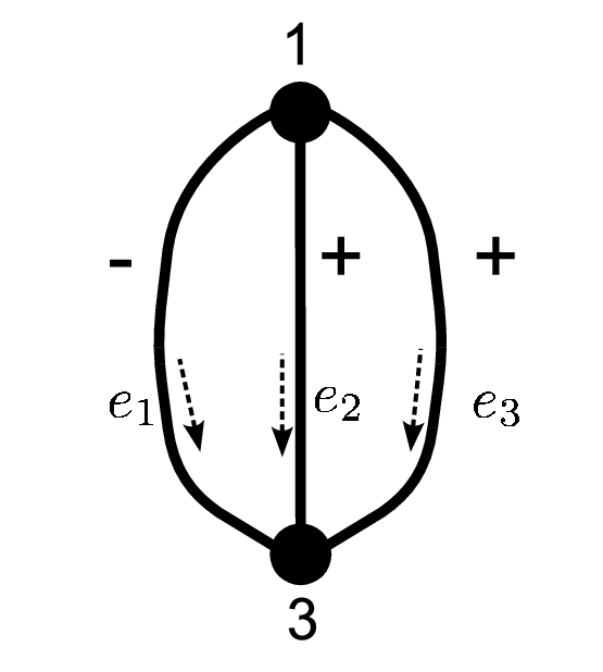
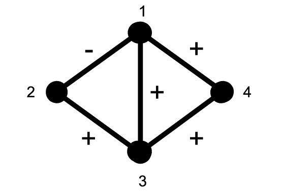
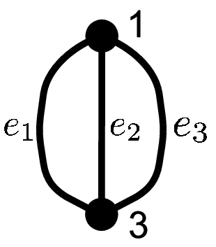
Let V:={1,2,3,4}V:=\{1,2,3,4\} and E:={12,13,14,23,34}E:=\{12,13,14,23,34\}. The interactions are given by arbitrary {hi}\{h_{i}\} and {−J12,J13,J14,J23,J34}\{-J_{12},J_{13},J_{14},J_{23},J_{34}\} with Ji​j≥0J_{ij}\geq 0. See figure 3. It is enough to check that det(I−ℬ​ℳ)>0\det(I-\mathcal{B}\mathcal{M})>0 for arbitrary 0≤β13,β23,β14,β34<10\leq\beta_{13},\beta_{23},\beta_{14},\beta_{34}<1 and −1<β12≤0-1<\beta_{12}\leq 0. Since the prime cycles of GG bijectively correspond to those of G^\hat{G} (in figure 3), we have det(I−ℬ​ℳ)=det(I−ℬ^​ℳ^)\det(I-\mathcal{B}\mathcal{M})=\det(I-\mathcal{\hat{B}}\mathcal{\hat{M}}), where β^e1=β12​β23\hat{\beta}_{e_{1}}=\beta_{12}\beta_{23}, β^e2=β13\hat{\beta}_{e_{2}}=\beta_{13}, and β^e3=β34\hat{\beta}_{e_{3}}=\beta_{34}. We see that det(I−ℬ^​ℳ^)=(1−β^e1​β^e2−β^e1​β^e3−β^e2​β^e3−2​β^e1​β^e2​β^e3)​(1−β^e1​β^e2−β^e1​β^e3−β^e2​β^e3+2​β^e1​β^e2​β^e3)>0\det(I-\mathcal{\hat{B}}\mathcal{\hat{M}})=(1-\hat{\beta}_{e_{1}}\hat{\beta}_{e_{2}}-\hat{\beta}_{e_{1}}\hat{\beta}_{e_{3}}-\hat{\beta}_{e_{2}}\hat{\beta}_{e_{3}}-2\hat{\beta}_{e_{1}}\hat{\beta}_{e_{2}}\hat{\beta}_{e_{3}})(1-\hat{\beta}_{e_{1}}\hat{\beta}_{e_{2}}-\hat{\beta}_{e_{1}}\hat{\beta}_{e_{3}}-\hat{\beta}_{e_{2}}\hat{\beta}_{e_{3}}+2\hat{\beta}_{e_{1}}\hat{\beta}_{e_{2}}\hat{\beta}_{e_{3}})>0. In other cases, we can reduce to the graph G^\hat{G} or the graphs in figure 3 similarly (see the supplementary material).

For attractive models, the fixed point of the LBP is not necessarily unique.

For graphs with multiple cycles, all the existing results on uniqueness make assumptions that upperbound |Ji​j||J_{ij}| essentially. In contrast, Corollary 4 applies to arbitrary strength of interactions if the graph has two cycles and the interactions are not attractive. It is noteworthy that, from Corollary 2, the Bethe free energy is non-convex in the situation of Corollary 4, while the fixed point is unique.
Refer to caption
Figure 1: Graph of Example 2.
Refer to caption
Figure 2: Graph G^\hat{G}.
Refer to caption
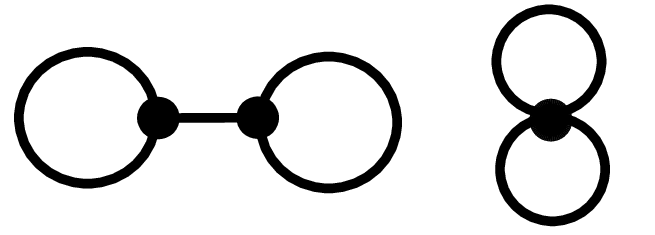
Figure 3: Two other types.

7 Concluding remarks

For binary pairwise models, we show the connection between the edge zeta function and the Bethe free energy in Theorem 3, in the proof of which the multi-variable version of Ihara’s formula (Theorem 2) is essential. After the initial submission of this paper, we found that Theorem 3 is extended to a more general class of models including multinomial models and Gaussian models represented by arbitrary factor graphs. We will discuss the extended formula and its applications in a future paper.

Some recent researches on LBP have suggested the importance of zeta function. In the context of the LDPC code, which is an important application of LBP, Koetter et al [21, 22] show the connection between pseudo-codewords and the edge zeta function. On the LBP for the Gaussian graphical model, Johnson et al [23] give zeta-like product formula of the partition function. While these are not directly related to our work, pursuing covered connections is an interesting future research topic.

Acknowledgements

This work was supported in part by Grant-in-Aid for JSPS Fellows 20-993 and Grant-in-Aid for Scientific Research (C) 19500249.

References

  • [1] J. Pearl. Probabilistic Reasoning in Intelligent Systems: Networks of Plausible Inference. Morgan Kaufmann Publishers, San Mateo, CA, 1988.
  • [2] K. Murphy, Y. Weiss, and M.I. Jordan. Loopy belief propagation for approximate inference: An empirical study. Proc. of Uncertainty in AI, 15:467–475, 1999.
  • [3] J.S. Yedidia, W.T. Freeman, and Y. Weiss. Generalized belief propagation. Adv. in Neural Information Processing Systems, 13:689–95, 2001.
  • [4] Y. Weiss. Correctness of Local Probability Propagation in Graphical Models with Loops. Neural Computation, 12(1):1–41, 2000.
  • [5] T. Heskes. On the uniqueness of loopy belief propagation fixed points. Neural Computation, 16(11):2379–2413, 2004.
  • [6] T. Heskes. Stable fixed points of loopy belief propagation are minima of the Bethe free energy. Adv. in Neural Information Processing Systems, 15, pages 343–350, 2002.
  • [7] K. Hashimoto. Zeta functions of finite graphs and representations of p-adic groups. Automorphic forms and geometry of arithmetic varieties, 15:211–280, 1989.
  • [8] H.M. Stark and A.A. Terras. Zeta functions of finite graphs and coverings. Advances in Mathematics, 121(1):124–165, 1996.
  • [9] Y. Ihara. On discrete subgroups of the two by two projective linear group over p-adic fields. Journal of the Mathematical Society of Japan, 18(3):219–235, 1966.
  • [10] H. Bass. The Ihara-Selberg zeta function of a tree lattice. Internat. J. Math, 3(6):717–97, 1992.
  • [11] P. Pakzad and V. Anantharam. Belief propagation and statistical physics. Conference on Information Sciences and Systems, (225), 2002.
  • [12] R.A. Horn and C.R. Johnson. Matrix analysis. Cambridge University Press, 1990.
  • [13] K. Hashimoto. On zeta and L-functions of finite graphs. Internat. J. Math, 1(4):381–396, 1990.
  • [14] J.M. Mooij and H.J. Kappen. On the properties of the Bethe approximation and loopy belief propagation on binary networks. J. Stat. Mech: Theory Exp., P11012, 2005.
  • [15] S. Ikeda, T. Tanaka, and S. Amari. Information geometry of turbo and low-density parity-check codes. IEEE Transactions on Information Theory, 50(6):1097–1114, 2004.
  • [16] C. Furtlehner, J.M. Lasgouttes, and A. De La Fortelle. Belief propagation and Bethe approximation for traffic prediction. INRIA RR-6144, Arxiv preprint physics/0703159, 2007.
  • [17] A.T. Ihler, JW Fisher, and A.S. Willsky. Loopy belief propagation: Convergence and effects of message errors. Journal of Machine Learning Research, 6(1):905–936, 2006.
  • [18] J. M. Mooij and H. J. Kappen. Sufficient Conditions for Convergence of the Sum-Product Algorithm. IEEE Transactions on Information Theory, 53(12):4422–4437, 2007.
  • [19] S. Tatikonda and M.I. Jordan. Loopy belief propagation and Gibbs measures. Uncertainty in AI, 18:493–500, 2002.
  • [20] B.A. Dubrovin, A.T. Fomenko, S.P. Novikov, and Burns R.G. Modern Geometry: Methods and Applications: Part 2: the Geometry and Topology of Manifolds . Springer-Verlag, 1985.
  • [21] R. Koetter, W.C.W. Li, PO Vontobel, and JL Walker. Pseudo-codewords of cycle codes via zeta functions. IEEE Information Theory Workshop, pages 6–12, 2004.
  • [22] R. Koetter, W.C.W. Li, P.O. Vontobel, and J.L. Walker. Characterizations of pseudo-codewords of (low-density) parity-check codes. Advances in Mathematics, 213(1):205–229, 2007.
  • [23] J.K. Johnson, V.Y. Chernyak, and M. Chertkov. Orbit-Product Representation and Correction of Gaussian Belief Propagation. Proc. of the 26th International Conference on Machine Learning, pages 473–480, 2009.
  • [24] C.D. Godsil and G. Royle. Algebraic Graph Theory. Springer, 2001.
  • [25] M. Kotani and T. Sunada. Zeta functions of finite graphs. J. Math. Sci. Univ. Tokyo, 7(1):7–25, 2000.
  • [26] S. Northshield. A note on the zeta function of a graph. Journal of Combinatorial Theory, Series B, 74(2):408–410, 1998.

Supplementary Material for
“Graph Zeta Function in the Bethe Free Energy and
Loopy Belief Propagation”
Yusuke Watanabe and Kenji Fukumizu, NIPS 2009


Appendix A Proof of Theorem 2

Proof.

First, we define three linear operators 𝒪:C⁡(V)→C⁡(E→)\mathcal{O}:C(V)\rightarrow C(\vec{E}), 𝒯∗:C⁡(E→)→C⁡(V)\mathcal{T}^{*}:C(\vec{E})\rightarrow C(V), and ι:C⁡(E→)→C⁡(E→)\iota:C(\vec{E})\rightarrow C(\vec{E}) as follows:

(𝒪​f)​(e):=f⁡(o⁡(e)),(𝒯∗​g)​(i):=∑e∈E→,t⁡(e)=ig⁡(e),(ι​g)​(e):=g⁡(e¯) where ​f∈C⁡(V)​ and ​g∈C⁡(E→).(\mathcal{O}f)(e):=f(o(e)),\quad(\mathcal{T}^{*}g)(i):=\hskip-11.38109pt\sum_{e\in\vec{E},t(e)=i}\hskip-8.53581ptg(e),\quad(\iota g)(e):=g(\bar{e})\quad\text{ where }f\in C(V)\text{ and }g\in C(\vec{E}).

We see that ℳ=𝒪​𝒯∗−ι\mathcal{M}=\mathcal{O}\mathcal{T}^{*}-\iota, because

((𝒪​𝒯∗−ι)​g)​(e)=∑e′∈E→,t⁡(e′)=o⁡(e)g⁡(e′)−g⁡(e¯)=(ℳ​g)​(e) for ​g∈C⁡(E→).\displaystyle\big((\mathcal{O}\mathcal{T}^{*}-\iota)g\big)(e)=\hskip-5.69054pt\sum_{e^{\prime}\in\vec{E},t(e^{\prime})=o(e)}\hskip-17.07164ptg(e^{\prime})\hskip 5.69054pt-g(\bar{e})=(\mathcal{M}g)(e)\quad\text{ for }g\in C(\vec{E}).

Then we have

det(I−𝒰​ℳ)\displaystyle\det(I-\mathcal{U}\mathcal{M}) =det(I−𝒰​𝒪​𝒯∗​(I+𝒰​ι)−1)​det(I+𝒰​ι)\displaystyle=\det\Big(I-\mathcal{U}\mathcal{O}\mathcal{T}^{*}(I+\mathcal{U}\iota)^{-1}\Big)\det(I+\mathcal{U}\iota)
=det(I−𝒯∗​(I+𝒰​ι)−1​𝒰​𝒪)​det(I+𝒰​ι).\displaystyle=\det\Big(I-\mathcal{T}^{*}(I+\mathcal{U}\iota)^{-1}\mathcal{U}\mathcal{O}\Big)\det(I+\mathcal{U}\iota).

In the second equality, we used det(In−A​B)=det(Im−B​A)\det(I_{n}-AB)=\det(I_{m}-BA) for n×mn\times m and m×nm\times n matrices AA and BB ([24], Lemma 8.2.4). The linear operator ι\iota is a block diagonal matrix with standard basis. The (e,e¯)(e,\bar{e}) block of I+𝒰​ιI+\mathcal{U}\iota is

[1ueue¯1].\begin{bmatrix}1&u_{e}\\ u_{\bar{e}}&1\end{bmatrix}.

Therefore, we have det(I+𝒰​ι)=∏[e]∈E(1−ue​ue¯)\det(I+\mathcal{U}\iota)=\prod_{[e]\in E}(1-u_{e}u_{\bar{e}}).

Finally, we check that 𝒯∗​(I+𝒰​ι)−1​𝒰​𝒪=𝒜^−𝒟^\mathcal{T}^{*}(I+\mathcal{U}\iota)^{-1}\mathcal{U}\mathcal{O}=\mathcal{\hat{A}}-\mathcal{\hat{D}}. The matrix (I+𝒰​ι)−1(I+\mathcal{U}\iota)^{-1} is a block diagonal matrix with (e,e¯)(e,\bar{e}) block

11−ue​ue¯​[1−ue−ue¯1].\frac{1}{1-u_{e}u_{\bar{e}}}\begin{bmatrix}1&-u_{e}\\ -u_{\bar{e}}&1\end{bmatrix}. (18)

For f∈C⁡(V)f\in C(V), we have

(𝒯∗​(I+𝒰​ι)−1​𝒰​𝒪​f)​(i)\displaystyle\Big(\mathcal{T}^{*}(I+\mathcal{U}\iota)^{-1}\mathcal{U}\mathcal{O}f\Big)(i) =∑e∈E→,t⁡(e)=i((I+𝒰​ι)−1​𝒰​𝒪​f)​(e)\displaystyle=\sum_{e\in\vec{E},t(e)=i}\Big((I+\mathcal{U}\iota)^{-1}\mathcal{U}\mathcal{O}f\Big)(e)
=∑e∈E→,t⁡(e)=i11−ue​ue¯​((𝒰​𝒪​f)​(e)−ue​(𝒰​𝒪​f)​(e¯))\displaystyle=\sum_{e\in\vec{E},t(e)=i}\frac{1}{1-u_{e}u_{\bar{e}}}\Big((\mathcal{U}\mathcal{O}f)(e)-u_{e}(\mathcal{U}\mathcal{O}f)(\bar{e})\Big)
=∑e∈E→,t⁡(e)=i11−ue​ue¯​(ue​f​(o⁡(e))−ue​ue¯​f​(o⁡(e¯)))\displaystyle=\sum_{e\in\vec{E},t(e)=i}\frac{1}{1-u_{e}u_{\bar{e}}}\Big(u_{e}f(o(e))-u_{e}u_{\bar{e}}f(o(\bar{e}))\Big)
=(𝒜^​f)​(i)−(𝒟^​f)​(i).\displaystyle=(\mathcal{\hat{A}}f)(i)-(\mathcal{\hat{D}}f)(i).

∎

Appendix B Proof of Theorem 3

B.1 Explicit formula of derivatives of the Bethe free energy

In the proof of Theorem 3, the graph G=(V,E)G=(V,E) is assumed to be a simple graph, i.e., there is no multiple edges and loop-edge

For the proof, we need explicit expressions of the second derivatives of the Bethe free energy. We list them below.

The first derivatives of the Bethe Free Energy are

∂F∂mi\displaystyle\frac{\partial F}{\partial m_{i}} =−hi+(1−di)​12​∑xi=±1xi​log⁡bi​(xi)+14​∑k∈Ni∑xi,xk=±1xi​log⁡bi​k​(xi,xk),\displaystyle=-h_{i}+(1-d_{i})\frac{1}{2}\sum_{x_{i}=\pm 1}x_{i}\log b_{i}(x_{i})+\frac{1}{4}\sum_{k\in N_{i}}\sum_{x_{i},x_{k}=\pm 1}x_{i}\log b_{ik}(x_{i},x_{k}), (19)
∂F∂χi​j\displaystyle\frac{\partial F}{\partial\chi_{ij}} =−Ji​j+14​∑xi,xj=±1xi​xj​log⁡bi​j​(xi,xj).\displaystyle=-J_{ij}+\frac{1}{4}\sum_{x_{i},x_{j}=\pm 1}x_{i}x_{j}\log b_{ij}(x_{i},x_{j}). (20)

The second derivatives of the Bethe Free Energy are

∂2F∂mi​∂mj\displaystyle\frac{\partial^{2}F}{\partial m_{i}\partial m_{j}} ={(1−di)​11−mi2+14​∑k∈Ni∑xi,xk11+mi​xi+mk​xk+χi​k​xi​xk if ​i=j,14​∑xi,xjxi​xj1+mi​xi+mj​xj+χi​j​xi​xj if ​i​ and ​j​ are adjacent ​(i≠j),0 otherwise,\displaystyle=\begin{cases}(1-d_{i})\frac{1}{1-m_{i}^{2}}+\frac{1}{4}\sum_{k\in N_{i}}\sum_{x_{i},x_{k}}\frac{1}{1+m_{i}x_{i}+m_{k}x_{k}+\chi_{ik}x_{i}x_{k}}\quad\text{ if }i=j,\\ \frac{1}{4}\sum_{x_{i},x_{j}}\frac{x_{i}x_{j}}{1+m_{i}x_{i}+m_{j}x_{j}+\chi_{ij}x_{i}x_{j}}\quad\text{ if }i\text{ and }j\text{ are adjacent }(i\neq j),\\ 0\hskip 133.72795pt\text{ otherwise,}\end{cases} (21)
∂2F∂mk​∂χi​j\displaystyle\frac{\partial^{2}F}{\partial m_{k}\partial\chi_{ij}} ={14​∑xi,xjxj1+mi​xi+mj​xj+χi​j​xi​xj if ​k=i,14​∑xi,xjxi1+mi​xi+mj​xj+χi​j​xi​xj if ​k=j,0 otherwise, \displaystyle=\begin{cases}\frac{1}{4}\sum_{x_{i},x_{j}}\frac{x_{j}}{1+m_{i}x_{i}+m_{j}x_{j}+\chi_{ij}x_{i}x_{j}}\quad\text{ if }k=i,\\ \frac{1}{4}\sum_{x_{i},x_{j}}\frac{x_{i}}{1+m_{i}x_{i}+m_{j}x_{j}+\chi_{ij}x_{i}x_{j}}\quad\text{ if }k=j,\\ 0\hskip 133.72795pt\text{ otherwise, }\\ \end{cases} (22)
∂2F∂χi​j​∂χk​l\displaystyle\frac{\partial^{2}F}{\partial\chi_{ij}\partial\chi_{kl}} ={14​∑xi​xj11+mi​xi+mj​xj+χi​j​xi​xj if ​i​j=k​l,0 otherwise. \displaystyle=\begin{cases}\frac{1}{4}\sum_{x_{i}x_{j}}\frac{1}{1+m_{i}x_{i}+m_{j}x_{j}+\chi_{ij}x_{i}x_{j}}\hskip 2.84526pt\quad\text{ if }ij=kl,\\ 0\hskip 133.72795pt\text{ otherwise. }\\ \end{cases} (23)

We use notations

ri​j:=14​∑xi,xj11+mi​xi+mj​xj+χi​j​xi​xj,\displaystyle r_{ij}:=\frac{1}{4}\sum_{x_{i},x_{j}}\frac{1}{1+m_{i}x_{i}+m_{j}x_{j}+\chi_{ij}x_{i}x_{j}}, (24)
si​j:=14​∑xi,xjxj1+mi​xi+mj​xj+χi​j​xi​xj,\displaystyle s_{ij}:=\frac{1}{4}\sum_{x_{i},x_{j}}\frac{x_{j}}{1+m_{i}x_{i}+m_{j}x_{j}+\chi_{ij}x_{i}x_{j}}, (25)
ti​j:=14​∑xi,xjxi​xj1+mi​xi+mj​xj+χi​j​xi​xj.\displaystyle t_{ij}:=\frac{1}{4}\sum_{x_{i},x_{j}}\frac{x_{i}x_{j}}{1+m_{i}x_{i}+m_{j}x_{j}+\chi_{ij}x_{i}x_{j}}. (26)

Note that ri​j=rj​ir_{ij}=r_{ji} and ti​j=tj​it_{ij}=t_{ji}, but si​j≠sj​is_{ij}\neq s_{ji} in general.

B.2 Detailed proof of Theorem 3

Proof.

First, note that the Hessian of the Bethe free energy is a square matrix of size N+MN+M:

∇2F​({mi,χi​j}):=[(∂2F∂mi​∂mj)(∂2F∂mi​∂χs​t)(∂2F∂χu​v​∂mj)(∂2F∂χu​v​∂χs​t)].\nabla^{2}F(\{m_{i},\chi_{ij}\}):=\begin{bmatrix}\Big(\frac{\partial^{2}F}{\partial m_{i}\partial m_{j}}\Big)&\Big(\frac{\partial^{2}F}{\partial m_{i}\partial\chi_{st}}\Big)\\ \Big(\frac{\partial^{2}F}{\partial\chi_{uv}\partial m_{j}}\Big)&\Big(\frac{\partial^{2}F}{\partial\chi_{uv}\partial\chi_{st}}\Big)\end{bmatrix}.

Recall that NN is the number of vertices and MM is the number of undirected edges.

Step1: Computation of Y
From (23), the (E,E)-block of the Hessian is a diagonal matrix given by

∂2F∂χi​j​∂χk​l=δi​j,k​l​ri​j.\frac{\partial^{2}F}{\partial\chi_{ij}\partial\chi_{kl}}=\delta_{ij,kl}r_{ij}.

Using this diagonal block, we erase (V,E)-block and (E,V)-block of the Hessian. Thus, we obtain a square matrix XX such that detX=1\det X=1 and

XT​(∇2F)​X=[Y00(∂2F∂χi​j​∂χk​l)].X^{T}(\nabla^{2}F)X=\begin{bmatrix}\quad Y&0\\ \quad 0&\Big(\frac{\partial^{2}F}{\partial\chi_{ij}\partial\chi_{kl}}\Big)\end{bmatrix}.

Applying an identity

(10−si​jri​j01−sj​iri​j001)​(witi​jsi​jti​jwjsj​isi​jsj​iri​j)​(100010−si​jri​j−sj​iri​j1)=(wi−si​j2ri​jti​j−si​j​sj​iri​j0ti​j−si​j​sj​iri​jwj−sj​i2ri​j000ri​j)\begin{pmatrix}1&0&\frac{-s_{ij}}{r_{ij}}\\ 0&1&\frac{-s_{ji}}{r_{ij}}\\ 0&0&1\end{pmatrix}\begin{pmatrix}w_{i}&t_{ij}&s_{ij}\\ t_{ij}&w_{j}&s_{ji}\\ s_{ij}&s_{ji}&r_{ij}\end{pmatrix}\begin{pmatrix}1&0&0\\ 0&1&0\\ \frac{-s_{ij}}{r_{ij}}&\frac{-s_{ji}}{r_{ij}}&1\end{pmatrix}=\begin{pmatrix}w_{i}-\frac{s_{ij}^{2}}{r_{ij}}&t_{ij}-\frac{s_{ij}s_{ji}}{r_{ij}}&0\\ t_{ij}-\frac{s_{ij}s_{ji}}{r_{ij}}&w_{j}-\frac{s_{ji}^{2}}{r_{ij}}&0\\ 0&0&r_{ij}\end{pmatrix}

for each edge, we have

(Y)i,j\displaystyle(Y)_{i,j} ={(1−di)​11−mi2+∑k∈Ni(ri​k−si​k2ri​k) if ​i=j,ti​j−si​j​sj​iri​j if ​i​ and ​j​ are adjacent ,0 otherwise.\displaystyle=\begin{cases}(1-d_{i})\frac{1}{1-m_{i}^{2}}+\sum_{k\in N_{i}}(r_{ik}-\frac{{s_{ik}^{2}}}{r_{ik}})\quad\text{ if }i=j,\\ t_{ij}-\frac{s_{ij}s_{ji}}{r_{ij}}\quad\text{ if }i\text{ and }j\text{ are adjacent },\\ 0\quad\qquad\qquad\text{ otherwise.}\end{cases}

The elements of YY are represented in terms of {mi,χi​j}\{m_{i},\chi_{ij}\} as follows:

(Y)i,i\displaystyle(Y)_{i,i} =11−mi2+∑k∈Ni(ri​k−si​k2ri​k−11−mi2)\displaystyle=\frac{1}{1-m_{i}^{2}}+\sum_{k\in N_{i}}(r_{ik}-\frac{{s_{ik}^{2}}}{r_{ik}}-\frac{1}{1-m_{i}^{2}})
=11−mi2+∑k∈Ni(χi​k−mi​mk)2(1−mi2)​(1−mi2−mk2+2​mi​mk​χi​k−χi​k2) and,\displaystyle=\frac{1}{1-m_{i}^{2}}+\sum_{k\in N_{i}}\frac{(\chi_{ik}-m_{i}m_{k})^{2}}{(1-m_{i}^{2})(1-m_{i}^{2}-m_{k}^{2}+2m_{i}m_{k}\chi_{ik}-\chi_{ik}^{2})}\quad\text{ and, }
(Y)i,j\displaystyle(Y)_{i,j} =ti​j−si​j​sj​iri​j\displaystyle=t_{ij}-\frac{s_{ij}s_{ji}}{r_{ij}}
=−(χi​j−mi​mj)(1−mi2−mj2+2​mi​mj​χi​j−χi​j2) for adjacent i and j.\displaystyle=\frac{-(\chi_{ij}-m_{i}m_{j})}{(1-m_{i}^{2}-m_{j}^{2}+2m_{i}m_{j}\chi_{ij}-\chi_{ij}^{2})}\quad\text{ for adjacent }i\text{ and }j.

Step2: Computation of IN+𝒟^−𝒜^I_{N}+\mathcal{\hat{D}}-\mathcal{\hat{A}}
From the definition (13) of uj→iu_{j\rightarrow i}, we see that

ui→j​uj→i1−ui→j​uj→i\displaystyle\frac{u_{i\rightarrow j}u_{j\rightarrow i}}{1-u_{i\rightarrow j}u_{j\rightarrow i}} =(χi​j−mi​mj)2(1−mi2−mj2+2​mi​mj​χi​j−χi​j2),\displaystyle=\frac{(\chi_{ij}-m_{i}m_{j})^{2}}{(1-m_{i}^{2}-m_{j}^{2}+2m_{i}m_{j}\chi_{ij}-\chi_{ij}^{2})},
ui→j1−ui→j​uj→i\displaystyle\frac{u_{i\rightarrow j}}{1-u_{i\rightarrow j}u_{j\rightarrow i}} =(1−mi2)​(χi​j−mi​mj)(1−mi2−mj2+2​mi​mj​χi​j−χi​j2).\displaystyle=\frac{(1-m_{i}^{2})(\chi_{ij}-m_{i}m_{j})}{(1-m_{i}^{2}-m_{j}^{2}+2m_{i}m_{j}\chi_{ij}-\chi_{ij}^{2})}.

Therefore, the diagonal element is

(IN+𝒟^−𝒜^)i,i=(IN+𝒟^)i,i\displaystyle(I_{N}+\mathcal{\hat{D}}-\mathcal{\hat{A}})_{i,i}=(I_{N}+\mathcal{\hat{D}})_{i,i} =1+∑k∈Niui→k​uk→i1−ui→k​uk→i\displaystyle=1+\sum_{k\in N_{i}}\frac{u_{i\rightarrow k}u_{k\rightarrow i}}{1-u_{i\rightarrow k}u_{k\rightarrow i}}
=1+∑k∈Ni(χi​k−mi​mk)2(1−mi2−mk2+2​mi​mk​χi​k−χi​k2),\displaystyle=1+\sum_{k\in N_{i}}\frac{(\chi_{ik}-m_{i}m_{k})^{2}}{(1-m_{i}^{2}-m_{k}^{2}+2m_{i}m_{k}\chi_{ik}-\chi_{ik}^{2})},

and for adjacent ii and jj,

(IN+𝒟^−𝒜^)i,j=−(𝒜^)i,j\displaystyle(I_{N}+\mathcal{\hat{D}}-\mathcal{\hat{A}})_{i,j}=-(\mathcal{\hat{A}})_{i,j} =−uj→i1−ui→j​uj→i\displaystyle=\frac{-u_{j\rightarrow i}}{1-u_{i\rightarrow j}u_{j\rightarrow i}}
=−(1−mj2)​(χi​j−mi​mj)(1−mi2−mj2+2​mi​mj​χi​j−χi​j2).\displaystyle=\frac{-(1-m_{j}^{2})(\chi_{ij}-m_{i}m_{j})}{(1-m_{i}^{2}-m_{j}^{2}+2m_{i}m_{j}\chi_{ij}-\chi_{ij}^{2})}.

Combining the results of step 1 and 2, we have

IN+𝒟^−𝒜^=Y⁡[1−m120…001−m22…0⋮⋮⋱⋮00…1−mN2].I_{N}+\mathcal{\hat{D}}-\mathcal{\hat{A}}=Y\left[\begin{array}[]{cccc}1-m_{1}^{2}&0&\ldots&0\\ 0&1-m_{2}^{2}&\dots&0\\ \vdots&\vdots&\ddots&\vdots\\ 0&0&\ldots&1-m_{N}^{2}\end{array}\right].

Step3: Final step
We see that

ζG​(𝒖)−1\displaystyle\zeta_{G}(\boldsymbol{u})^{-1} =det(I−𝒰​ℳ)\displaystyle=\det(I-\mathcal{U}\mathcal{M}) (27)
=det(IN+𝒟^−𝒜^)​∏[e]∈E(1−ue​ue¯)\displaystyle=\det(I_{N}+\mathcal{\hat{D}}-\mathcal{\hat{A}})\prod_{[e]\in E}(1-u_{e}u_{\bar{e}}) (28)
=det(Y)​∏i∈V(1−mi2)​∏[e]∈E(1−ue​ue¯)\displaystyle=\det(Y)\prod_{i\in V}(1-m_{i}^{2})\prod_{[e]\in E}(1-u_{e}u_{\bar{e}})
=det(∇2F)​∏i∈V(1−mi2)​∏i​j∈E1−ui→j​uj→iri​j\displaystyle=\det(\nabla^{2}F)\prod_{i\in V}(1-m_{i}^{2})\prod_{ij\in E}\frac{1-u_{i\rightarrow j}u_{j\rightarrow i}}{r_{ij}}
=det(∇2F)​∏i∈V(1−mi2)1−di​∏i​j∈E(1−ui→j​uj→i)​(1−mi2)​(1−mj2)ri​j.\displaystyle=\det(\nabla^{2}F)\prod_{i\in V}(1-m_{i}^{2})^{1-d_{i}}\prod_{ij\in E}\frac{(1-u_{i\rightarrow j}u_{j\rightarrow i})(1-m_{i}^{2})(1-m_{j}^{2})}{r_{ij}}. (29)

From (27) to (28), we used the edge zeta version of Ihara’s formula (Theorem 2).

Furthermore, with a straightforward computation we see that

(1−ui→j​uj→i)​(1−mi2)​(1−mj2)ri​j=44​∏xi,xj=±1bi​j​(xi,xj),\displaystyle\frac{(1-u_{i\rightarrow j}u_{j\rightarrow i})(1-m_{i}^{2})(1-m_{j}^{2})}{r_{ij}}=4^{4}\prod_{x_{i},x_{j}=\pm 1}b_{ij}(x_{i},x_{j}),
(1−mi2)1−di=22−2​di​∏xi=±1bi​(xi)1−di,\displaystyle(1-m_{i}^{2})^{1-d_{i}}=2^{2-2d_{i}}\prod_{x_{i}=\pm 1}b_{i}(x_{i})^{1-d_{i}},

where bi​j​(xi,xj)=14​(1+mi​xi+mj​xj+χi​j​xi​xj)b_{ij}(x_{i},x_{j})=\frac{1}{4}(1+m_{i}x_{i}+m_{j}x_{j}+\chi_{ij}x_{i}x_{j}) and bi​(xi)=12​(1+mi)b_{i}(x_{i})=\frac{1}{2}(1+m_{i}).

Therefore,

(29) =2∑i∈V(2−2​di)​44​M​det(∇2F)​∏i∈V∏xi=±1bi​(xi)1−di​∏i​j∈E∏xi,xj=±1bi​j​(xi,xj)\displaystyle=2^{\sum_{i\in V}(2-2d_{i})}4^{4M}\det(\nabla^{2}F)\prod_{i\in V}\prod_{x_{i}=\pm 1}b_{i}(x_{i})^{1-d_{i}}\prod_{ij\in E}\prod_{x_{i},x_{j}=\pm 1}b_{ij}(x_{i},x_{j})
=22​N+4​M​det(∇2F)​∏i∈V∏xi=±1bi​(xi)1−di​∏i​j∈E∏xi,xj=±1bi​j​(xi,xj).\displaystyle=2^{2N+4M}\det(\nabla^{2}F)\prod_{i\in V}\prod_{x_{i}=\pm 1}b_{i}(x_{i})^{1-d_{i}}\prod_{ij\in E}\prod_{x_{i},x_{j}=\pm 1}b_{ij}(x_{i},x_{j}).

∎

Appendix C Proof of Corollary 2

Here, we prove the limit formula in Corollary 2.

Proof.

We can easily check that ui→j​(t)=tu_{i\rightarrow j}(t)=t,

∏i​j∈E∏xi,xj=±1bi​j​(xi,xj)=4−4​M​(1−t)2​M​(1+t)2​M, and\displaystyle\prod_{ij\in E}\prod_{x_{i},x_{j}=\pm 1}b_{ij}(x_{i},x_{j})=4^{-4M}(1-t)^{2M}(1+t)^{2M},\text{ and}
∏i∈V∏xi=±1bi​(xi)1−di=2−2​N+4​M\displaystyle\prod_{i\in V}\prod_{x_{i}=\pm 1}b_{i}(x_{i})^{1-d_{i}}=2^{-2N+4M}

on this interval. Therefore

limt→1det(∇2F​(t))​(1−t)M+N−1\displaystyle\lim_{t\rightarrow 1}\det(\nabla^{2}F(t))(1-t)^{M+N-1} =limt→1ζG​(𝒖⁡(t))−1​(1−t)M+N−1\displaystyle=\lim_{t\rightarrow 1}\zeta_{G}(\boldsymbol{u}(t))^{-1}(1-t)^{M+N-1}
(4−4​M​(1−t)2​M​(1+t)2​M​2−2​N+4​M​22​N+4​M)−1\displaystyle\qquad\Big(4^{-4M}(1-t)^{2M}(1+t)^{2M}2^{-2N+4M}2^{2N+4M}\Big)^{-1}
=limt→1ζG​(t)−1​(1−t)−M+N−1​2−2​M\displaystyle=\lim_{t\rightarrow 1}\zeta_{G}(t)^{-1}(1-t)^{-M+N-1}2^{-2M}
=−(M−N)​κ​(G)​2−M−N+1.\displaystyle=-(M-N)\kappa(G)2^{-M-N+1}.

On the final equality, we used Hashimoto’s formula:

limu→1ζG​(u)−1​(1−u)−M+N−1=−2M−N+1​(M−N)​κ​(G).\lim_{u\rightarrow 1}\zeta_{G}(u)^{-1}(1-u)^{-M+N-1}=-2^{M-N+1}(M-N)\kappa(G).

We refer to [13, 25, 26] for this formula. ∎

Appendix D Transformation of messages and proof of Theorem 5

D.1 Transformation of messages

First, we make an easy observation on the LBP update.

Proposition 1.

Let {πi→j}\{\pi_{i\rightarrow j}\} be any set of messages. We define a transformation from messages {μi→jt}\{{\mu}^{t}_{i\rightarrow j}\} to messages {μ~i→jt}\{\tilde{\mu}^{t}_{i\rightarrow j}\} by

μ~i→jt​(xj)∝μi→jt​(xj)πi→j​(xj).\tilde{\mu}^{t}_{i\rightarrow j}(x_{j})\propto\frac{\mu^{t}_{i\rightarrow j}(x_{j})}{\pi_{i\rightarrow j}(x_{j})}. (30)

We also define transformation from functions {ψi​j,ψi}\{\psi_{ij},\psi_{i}\} to functions {ψ~i​j,ψ~i}\{\tilde{\psi}_{ij},\tilde{\psi}_{i}\} by

ψ~i​j​(xi,xj)∝ψi​j​(xi,xj)πi→j​(xj)​πj→i​(xi),\displaystyle\tilde{\psi}_{ij}(x_{i},x_{j})\propto\frac{\psi_{ij}(x_{i},x_{j})}{\pi_{i\rightarrow j}(x_{j})\pi_{j\rightarrow i}(x_{i})}, (31)
ψ~i​(xi)∝ψi​(xi)​∏k∈Niπk→i​(xi).\displaystyle\tilde{\psi}_{i}(x_{i})\propto\psi_{i}(x_{i})\prod_{k\in N_{i}}\pi_{k\rightarrow i}(x_{i}). (32)

Then the update

μi→jt+1​(xj)∝∑xiψj​i​(xj,xi)​ψi​(xi)​∏k∈Ni∖jμk→it​(xi),\mu^{t+1}_{i\rightarrow j}(x_{j})\propto\sum_{x_{i}}\psi_{ji}(x_{j},x_{i})\psi_{i}(x_{i})\prod_{k\in N_{i}\setminus j}\mu^{t}_{k\rightarrow i}(x_{i}),\vskip-2.84526pt (33)

is equivalent to

μ~i→jt+1​(xj)∝∑xiψ~j​i​(xj,xi)​ψ~i​(xi)​∏k∈Ni∖jμ~k→it​(xi).\tilde{\mu}^{t+1}_{i\rightarrow j}(x_{j})\propto\sum_{x_{i}}\tilde{\psi}_{ji}(x_{j},x_{i})\tilde{\psi}_{i}(x_{i})\prod_{k\in N_{i}\setminus j}\tilde{\mu}^{t}_{k\rightarrow i}(x_{i}).\vskip-2.84526pt (34)
Proof.

The equivalence of (33) and (34) is easily checked by (30), (31), and (32). ∎

Symbolically, Proposition 1 implies that

Π∘T∘Π−1=T~,\Pi\circ T\circ\Pi^{-1}=\tilde{T}, (35)

where Π\Pi is the transformation of the messages by πi→j\pi_{i\rightarrow j}, TT is the LBP update with {ψi​j,ψi}\{\psi_{ij},\psi_{i}\}, and T~\tilde{T} is the LBP update with {ψ~i​j,ψ~i}\{\tilde{\psi}_{ij},\tilde{\psi}_{i}\} . Differentiation of this relation gives the transformation of the linearization matrix.

If we choose {πi→j}\{\pi_{i\rightarrow j}\} as πi→j​(xj)=μi→j∞​(xj)\pi_{i\rightarrow j}(x_{j})=\mu^{\infty}_{i\rightarrow j}(x_{j}), then (30), (31) and (32) becomes

μ~i→jt​(xj)∝μi→jt​(xj)μi→j∞​(xj)\displaystyle\tilde{\mu}^{t}_{i\rightarrow j}(x_{j})\propto\frac{\mu^{t}_{i\rightarrow j}(x_{j})}{\mu^{\infty}_{i\rightarrow j}(x_{j})} (36)
ψ~i​j​(xi,xj)∝bi​j​(xi,xj)bi​(xi)​bj​(xj)\displaystyle\tilde{\psi}_{ij}(x_{i},x_{j})\propto\frac{b_{ij}(x_{i},x_{j})}{b_{i}(x_{i})b_{j}(x_{j})} (37)
ψ~i​(xi)∝bi​(xi).\displaystyle\tilde{\psi}_{i}(x_{i})\propto b_{i}(x_{i}). (38)

This is the transformation used in the paper.

D.2 Proof of Theorem 5

Proof.

Let {μi→j∞​(xj)}\{\mu^{\infty}_{i\rightarrow j}(x_{j})\} be the set of messages at the fixed point and let Π\Pi be the transformation of messages defined by the fixed point messages. We parameterize the messages by ηi→jt=μi→jt​(+)/μi→jt​(−)\eta_{i\rightarrow j}^{t}=\mu^{t}_{i\rightarrow j}(+)/\mu^{t}_{i\rightarrow j}(-). It is enough to prove the assertion after the transformation and in this parameterization, because these operations cause similar linearization matrices.

After the transformation, the LBP update is given in terms of η~\tilde{\eta} as follows:

η~i→jt+1\displaystyle\tilde{\eta}^{t+1}_{i\rightarrow j} =∑xiψ~j​i​(+,xi)​ψi~​(xi)​∏k∈Ni∖jμ~k→i​(xi)∑xiψ~j​i​(−,xi)​ψi~​(xi)​∏k∈Ni∖jμ~k→i​(xi)\displaystyle=\frac{\sum_{x_{i}}\tilde{\psi}_{ji}(+,x_{i})\tilde{\psi_{i}}(x_{i})\prod_{k\in N_{i}\setminus j}\tilde{\mu}_{k\rightarrow i}(x_{i})}{\sum_{x_{i}}\tilde{\psi}_{ji}(-,x_{i})\tilde{\psi_{i}}(x_{i})\prod_{k\in N_{i}\setminus j}\tilde{\mu}_{k\rightarrow i}(x_{i})}
=bj​i​(+,+)bj​(+)​∏k∈Ni∖jη~k→i​(xi)+bj​i​(+,−)bj​(+)bj​i​(−,+)bj​(−)​∏k∈Ni∖jη~k→i​(xi)+bj​i​(−,−)bj​(−).\displaystyle=\frac{\frac{b_{ji}(+,+)}{b_{j}(+)}\prod_{k\in N_{i}\setminus j}\tilde{\eta}_{k\rightarrow i}(x_{i})+\frac{b_{ji}(+,-)}{b_{j}(+)}}{\frac{b_{ji}(-,+)}{b_{j}(-)}\prod_{k\in N_{i}\setminus j}\tilde{\eta}_{k\rightarrow i}(x_{i})+\frac{b_{ji}(-,-)}{b_{j}(-)}}.

Let 𝜼~∞:=Π⁡(𝜼∞){\boldsymbol{\tilde{\eta}}^{\infty}}:=\Pi(\boldsymbol{\eta}^{\infty}), then η~e∞=1\tilde{\eta}^{\infty}_{e}=1 for all e∈E→e\in\vec{E}. We can compute T′~​(𝜼~∞)\tilde{T^{\prime}}({\boldsymbol{\tilde{\eta}}^{\infty}}) as follows:

T′~​(𝜼~∞)\displaystyle\tilde{T^{\prime}}({\boldsymbol{\tilde{\eta}}^{\infty}}) =∂η~i→jt+1∂η~k→lt|𝜼~t=1\displaystyle=\frac{\partial\tilde{\eta}^{t+1}_{i\rightarrow j}}{\partial\tilde{\eta}^{t}_{k\rightarrow l}}\Big|_{\boldsymbol{\tilde{\eta}}^{t}=1}
=(bj​i​(+,+)bj​(+)−bj​i​(−,+)bj​(−))​ℳi→j,k→l\displaystyle=\Big(\frac{b_{ji}(+,+)}{b_{j}(+)}-\frac{b_{ji}(-,+)}{b_{j}(-)}\Big)\mathcal{M}_{i\rightarrow j,k\rightarrow l}
=χi​j−mi​mj1−mj2​ℳi→j,k→l.\displaystyle=\frac{\chi_{ij}-m_{i}m_{j}}{1-m_{j}^{2}}\mathcal{M}_{i\rightarrow j,k\rightarrow l}.

∎

Appendix E Idea and proof of Theorem 7

E.1 Idea of Theorem 7

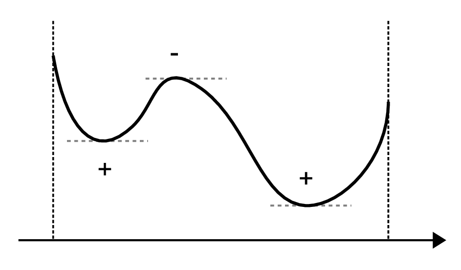
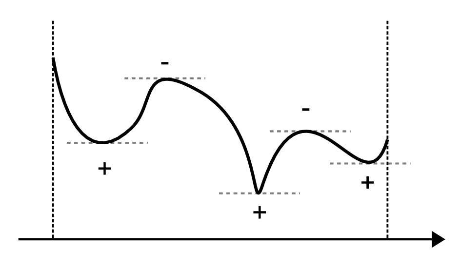
In Theorem 7, we show that the sum of indexes is equal to one. This is not so special. The simplest example that illustrate the idea of the theorem is sketched in figure 5. For each stationary point, plus or minus sign is assigned depending on the sign of the second derivative. When we deform the function, the sum is still equal to one as long as the outward gradients are positive at the boundaries. (See figure 5.)

Lemma 1, combined with Lemma 2, describes the behavior of the Bethe free energy near the boundary of L⁡(G)L(G).

Refer to caption
Figure 4: The sum of indexes is one.
Refer to caption
Figure 5: The sum of indexes is still one.

E.2 Proof of Lemma 1

Proof.

First, note that it is enough to prove the assertion when hi=0h_{i}=0 and Ji​j=0J_{ij}=0.

We prove by contradiction. Assume that ∥∇F​(qn)∥↛∞\lVert\nabla F(q_{n})\rVert\not\rightarrow\infty. Then, there exists R>0R>0 such that ∥∇F​(qn)∥≤R\lVert\nabla F(q_{n})\rVert\leq R for infinitely many nn. Let B0​(R)B_{0}(R) be the closed ball of radius RR centered at the origin. Taking subsequences, if necessary, we can assume that

∇F(qn)→(𝝃𝜼)∃∈B0(R),\nabla F(q_{n})\rightarrow{}^{\exists}\binom{\boldsymbol{\xi}}{\boldsymbol{\eta}}\in B_{0}(R), (39)

because of the compactness of B0​(R)B_{0}(R). Let bi​j(n)​(xi,xj)b_{ij}^{(n)}(x_{i},x_{j}) and bi(n)​(xi)b_{i}^{(n)}(x_{i}) be the pseudomarginals corresponding to qnq_{n}. Since qn→q∗∈∂L⁡(G)q_{n}\rightarrow q_{*}\in\partial L(G), there exist i​j∈Eij\in E, xix_{i} and xjx_{j} such that

bi​j(n)​(xi,xj)→0.b_{ij}^{(n)}(x_{i},x_{j})\rightarrow 0.

Without loss of generality, we assume that xi=+1x_{i}=+1 and xj=+1x_{j}=+1. From (39), we have

∇F(qn)i​j=14logbi​j(n)​(+,+)​bi​j(n)​(−,−)bi​j(n)​(+,−)​bi​j(n)​(−,+)⟶ηi​j.\nabla F(q_{n})_{ij}=\frac{1}{4}\log\frac{b_{ij}^{(n)}(+,+)b_{ij}^{(n)}(-,-)}{b_{ij}^{(n)}(+,-)b_{ij}^{(n)}(-,+)}\longrightarrow\eta_{ij}. (40)

Therefore bi​j(n)​(+,−)→0b_{ij}^{(n)}(+,-)\rightarrow 0 or bi​j(n)​(−,+)→0b_{ij}^{(n)}(-,+)\rightarrow 0 holds; we assume bi​j(n)​(+,−)→0b_{ij}^{(n)}(+,-)\rightarrow 0 without loss of generality. Now we have

bi(n)​(+)=bi​j(n)​(+,−)+bi​j(n)​(+,+)→0.b_{i}^{(n)}(+)=b_{ij}^{(n)}(+,-)+b_{ij}^{(n)}(+,+)\rightarrow 0.

In this situation, the following claim holds.

Claim.

Let k∈Nik\in N_{i}. In the limit of n→∞n\rightarrow\infty,

∑xi,xk=±1xi​log⁡bi​k(n)​(xi,xk)bi(n)​(xi)=log⁡[bi​k(n)​(+,+)​bi​k(n)​(+,−)​bi(n)​(−)2bi​k(n)​(−,+)​bi​k(n)​(−,−)​bi(n)​(+)2]\sum_{x_{i},x_{k}=\pm 1}x_{i}\log\frac{b^{(n)}_{ik}(x_{i},x_{k})}{b^{(n)}_{i}(x_{i})}=\log\left[\frac{b_{ik}^{(n)}(+,+)b_{ik}^{(n)}(+,-)b_{i}^{(n)}(-)^{2}}{b_{ik}^{(n)}(-,+)b_{ik}^{(n)}(-,-)b_{i}^{(n)}(+)^{2}}\right] (41)

converges to a finite value.

proof of claim.

From bi(n)​(+)→0b_{i}^{(n)}(+)\rightarrow 0, we have

bi​k(n)​(+,−),bi​k(n)​(+,+)⟶0 and bi(n)​(−)→1.b_{ik}^{(n)}(+,-),b_{ik}^{(n)}(+,+)\longrightarrow 0\quad\text{ and }\quad b_{i}^{(n)}(-)\rightarrow 1.

Case 1: bi​k(n)​(−,+)⟶bi​k∗​(−,+)≠0b_{ik}^{(n)}(-,+)\longrightarrow b_{ik}^{*}(-,+)\neq 0 and bi​k(n)​(−,−)⟶bi​k∗​(−,−)≠0b_{ik}^{(n)}(-,-)\longrightarrow b_{ik}^{*}(-,-)\neq 0.
In the same way as (40),

∇F(qn)i​k=14logbi​k(n)​(+,+)​bi​k(n)​(−,−)bi​k(n)​(+,−)​bi​k(n)​(−,+)⟶ηi​k.\nabla F(q_{n})_{ik}=\frac{1}{4}\log\frac{b_{ik}^{(n)}(+,+)b_{ik}^{(n)}(-,-)}{b_{ik}^{(n)}(+,-)b_{ik}^{(n)}(-,+)}\longrightarrow\eta_{ik}.

Therefore

bi​k(n)​(+,+)bi​k(n)​(+,−)⟶∃r≠0.\frac{b_{ik}^{(n)}(+,+)}{b_{ik}^{(n)}(+,-)}\longrightarrow{}^{\exists}r\neq 0.

Then we see that (41) converges to a finite value.

Case 2: bi​k(n)​(−,+)⟶1b_{ik}^{(n)}(-,+)\longrightarrow 1 and bi​k(n)​(−,−)⟶0b_{ik}^{(n)}(-,-)\longrightarrow 0.
Similar to the case 1, we have

bi​k(n)​(+,+)​bi​k(n)​(−,−)bi​k(n)​(+,−)⟶∃r≠0.\frac{b_{ik}^{(n)}(+,+)b_{ik}^{(n)}(-,-)}{b_{ik}^{(n)}(+,-)}\longrightarrow{}^{\exists}r\neq 0.

Therefore bi​k(n)​(+,−)bi​k(n)​(+,+)→0\frac{b_{ik}^{(n)}(+,-)}{b_{ik}^{(n)}(+,+)}\rightarrow 0. This implies that bi(n)​(+)bi​k(n)​(+,+)→1\frac{b_{i}^{(n)}(+)}{b_{ik}^{(n)}(+,+)}\rightarrow 1. Then we see that (41) converges to a finite value.

Case 3: bi​k(n)​(−,+)⟶0b_{ik}^{(n)}(-,+)\longrightarrow 0 and bi​k(n)​(−,−)⟶1b_{ik}^{(n)}(-,-)\longrightarrow 1.
Same as the case 2. ∎

Now let us get back to the proof of Lemma 1. We rewrite (19) as

∇F(qn)i=12logbi(n)(+)−12logbi(n)(−)+14∑k∈Ni∑xi,xk=±1xilogbi​k(n)​(xi,xk)bi(n)​(xi)\nabla F(q_{n})_{i}=\frac{1}{2}\log b^{(n)}_{i}(+)-\frac{1}{2}\log b^{(n)}_{i}(-)+\frac{1}{4}\sum_{k\in N_{i}}\sum_{x_{i},x_{k}=\pm 1}x_{i}\log\frac{b^{(n)}_{ik}(x_{i},x_{k})}{b^{(n)}_{i}(x_{i})} (42)

From (39), this value converges to ξi\xi_{i}. The second and the third terms in (42) converges to a finite value, while the first value converges to infinite. This is a contradiction. ∎

E.3 Detailed proof of Theorem 7

Proof.

Define a map Φ:L⁡(G)→ℝN+M\Phi:L(G)\rightarrow\mathbb{R}^{N+M} by

Φ​(q)i\displaystyle\Phi(q)_{i} =(1−di)​12​∑xi=±1xi​log⁡bi​(xi)+14​∑k∈Ni∑xi,xk=±1xi​log⁡bi​k​(xi,xk),\displaystyle=(1-d_{i})\frac{1}{2}\sum_{x_{i}=\pm 1}x_{i}\log b_{i}(x_{i})+\frac{1}{4}\sum_{k\in N_{i}}\sum_{x_{i},x_{k}=\pm 1}x_{i}\log b_{ik}(x_{i},x_{k}), (43)
Φ​(q)i​j\displaystyle\Phi(q)_{ij} =14​∑xi,xj=±1xi​xj​log⁡bi​j​(xi,xj),\displaystyle=\frac{1}{4}\sum_{x_{i},x_{j}=\pm 1}x_{i}x_{j}\log b_{ij}(x_{i},x_{j}), (44)

where bi​j​(xi,xj)b_{ij}(x_{i},x_{j}) and bi​(xi)b_{i}(x_{i}) are given by q={mi,χi​j}∈L⁡(G)q=\{m_{i},\chi_{ij}\}\in L(G). Therefore, we have ∇F=Φ−(𝒉𝑱)\nabla F=\Phi-\binom{\boldsymbol{h}}{\boldsymbol{J}} and ∇Φ=∇2F\nabla\Phi=\nabla^{2}F. Then following claim holds.

Claim.

The sets Φ−1​((𝐡𝐉)),Φ−1​(0)⊂L⁡(G)\Phi^{-1}(\binom{\boldsymbol{h}}{\boldsymbol{J}}),\Phi^{-1}(0)\subset L(G) are finite and

∑q∈Φ−1​(hJ)sgn(det∇Φ​(q))=∑q∈Φ−1​(0)sgn(det∇Φ​(q)),\sum_{q\in\Phi^{-1}({h\atop J})}\sgn(\det\nabla\Phi(q))=\sum_{q\in\Phi^{-1}(0)}\sgn(\det\nabla\Phi(q)), (45)

holds.

Before the proof of this claim, we prove Theorem 7 under the claim.

From (43) and (44), it is easy to see that Φ⁡(q)=0⇔q={mi=0,χi​j=0}\Phi(q)=0\Leftrightarrow q=\{m_{i}=0,\chi_{ij}=0\}. At this point, we can easily check that ∇Φ=∇2F\nabla\Phi=\nabla^{2}F is a positive definite matrix. Therefore the right hand side of (45) is equal to one. The left hand side of (45) is equal to the left hand side of (), because q∈Φ−1​((𝒉𝑱))⇔∇F​(q)=0q\in\Phi^{-1}(\binom{\boldsymbol{h}}{\boldsymbol{J}})\Leftrightarrow\nabla F(q)=0. Then the assertion of Theorem 7 is proved. ∎

Proof of the claim.

First, we prove that Φ−1​((𝒉𝑱))=(∇F)−1​(0)\Phi^{-1}(\binom{\boldsymbol{h}}{\boldsymbol{J}})=(\nabla F)^{-1}(0) is a finite set. If not, we can choose a sequence {qn}\{q_{n}\} of distinct points from this set. Let L⁡(G)¯\overline{L(G)} be the closure of L⁡(G)L(G). Since L⁡(G)¯\overline{L(G)} is compact, we can choose a subsequence that converges to some point q∗∈L⁡(G)¯q_{*}\in\overline{L(G)}. From Lemma 1, q∗∈L⁡(G)q_{*}\in L(G) and ∇F​(q∗)=0\nabla F(q_{*})=0 hold. By the assumption in Theorem 7, we have det∇2F​(q∗)≠0\det\nabla^{2}F(q_{*})\neq 0. This implies that ∇F​(q)≠0\nabla F(q)\neq 0 in some neighborhood of q∗q_{*}. This is a contradiction because qn→q∗q_{n}\rightarrow q_{*}.

Secondly, we prove the equality (45) using Lemma 2. Define a sequence of compact convex sets Cn:={q∈L(G)|∑i​j∈E∑xi,xj−logbi​j≤n}C_{n}:=\{q\in L(G)|\sum_{ij\in E}\sum_{x_{i},x_{j}}-\log b_{ij}\leq n\}, which increasingly converges to L⁡(G)L(G). Since Φ−1​(0)\Phi^{-1}(0) and Φ−1​(𝒉𝑱)\Phi^{-1}\binom{\boldsymbol{h}}{\boldsymbol{J}} are finite, they are included in CnC_{n} for sufficiently large nn. Take K>0K>0 and ϵ>0\epsilon>0 to satisfy K−ϵ>∥(𝒉𝑱)∥K-\epsilon>\lVert\binom{\boldsymbol{h}}{\boldsymbol{J}}\rVert. From Lemma 1, we see that Φ⁡(∂Cn)∩B0​(K)=ϕ\Phi(\partial C_{n})\cap B_{0}(K)=\phi for sufficiently large nn. Let non_{o} be such a large number. Let Πϵ:ℝN+M→B0​(K)\Pi_{\epsilon}:\mathbb{R}^{N+M}\rightarrow B_{0}(K) be a smooth map that is identity on B0​(K−ϵ)B_{0}(K-\epsilon), monotonically increasing on ∥x∥\lVert x\rVert, and Πϵ​(x)=K∥x∥​x\Pi_{\epsilon}(x)=\frac{K}{\lVert x\rVert}x for ∥x∥≥K\lVert x\rVert\geq K. Then we obtain a composition map Φ~:=Πϵ∘Φ:Cn0→B0​(K)\tilde{\Phi}:=\Pi_{\epsilon}\circ\Phi:C_{n_{0}}\rightarrow B_{0}(K) that satisfy Φ~​(∂Cn0)⊂∂B0​(K)\tilde{\Phi}(\partial C_{n_{0}})\subset\partial B_{0}(K). By definition, we have Φ−1​(0)=Φ~−1​(0)\Phi^{-1}(0)=\tilde{\Phi}^{-1}(0) and Φ−1​(𝒉𝑱)=Φ~−1​(𝒉𝑱)\Phi^{-1}\binom{\boldsymbol{h}}{\boldsymbol{J}}=\tilde{\Phi}^{-1}\binom{\boldsymbol{h}}{\boldsymbol{J}}. Therefore, both 00 and (𝒉𝑱)\binom{\boldsymbol{h}}{\boldsymbol{J}} are regular values of Φ~\tilde{\Phi}. From Lemma 2, we have

∑q∈Φ~−1​(hJ)sgn(det∇Φ~​(q))=∑q∈Φ~−1​(0)sgn(det∇Φ~​(q)).\sum_{q\in\tilde{\Phi}^{-1}({h\atop J})}\sgn(\det\nabla\tilde{\Phi}(q))=\sum_{q\in\tilde{\Phi}^{-1}(0)}\sgn(\det\nabla\tilde{\Phi}(q)).

Then, the assertion of the claim is proved. ∎

Appendix F Proof of Corollary 4

F.1 Detailed proof of Example 2

Refer to caption
Figure 6: The graph GG.
Refer to caption
Figure 7: The graph G^\hat{G}.

In this subsection we prove the assertion of Corollary 4 for the graph of Example 2, which is displayed in figure 7. The ++ and −- signs represent that of two body interactions.

It is enough to check that det(I−ℬ​ℳ)>0\det(I-\mathcal{B}\mathcal{M})>0 for arbitrary 0≤β13,β23,β14,β34<10\leq\beta_{13},\beta_{23},\beta_{14},\beta_{34}<1 and −1<β12≤0-1<\beta_{12}\leq 0. The graph G^\hat{G} in figure 7 is obtained by erasing vertices 22 and 44 in GG. To compute det(I−ℬ​ℳ)\det(I-\mathcal{B}\mathcal{M}), it is enough to consider G^\hat{G}. In fact

det(I−ℬ​ℳ)\displaystyle\det(I-\mathcal{B}\mathcal{M}) =ζG​(𝜷)−1\displaystyle=\zeta_{G}(\boldsymbol{\beta})^{-1}
=∏𝔭∈P(1−g⁡(𝔭))\displaystyle=\prod_{\mathfrak{p}\in P}(1-g(\mathfrak{p})) (46)
=∏𝔭^∈P^(1−g⁡(𝔭^))\displaystyle=\prod_{\mathfrak{\hat{p}}\in\hat{P}}(1-g(\mathfrak{\hat{p}})) (47)
=ζG^​(𝜷^)−1=det(I−ℬ^​ℳ^),\displaystyle=\zeta_{\hat{G}}(\boldsymbol{\hat{\beta}})^{-1}=\det(I-\mathcal{\hat{B}}\mathcal{\hat{M}}),

where β^e1:=β12​β23\hat{\beta}_{e_{1}}:=\beta_{12}\beta_{23}, β^e2:=β13\hat{\beta}_{e_{2}}:=\beta_{13}, β^e3:=β14​β34\hat{\beta}_{e_{3}}:=\beta_{14}\beta_{34} and β^ei=β^ei¯\hat{\beta}_{e_{i}}=\hat{\beta}_{\bar{e_{i}}}. The equality between (46) and (47) is obtained by the one to one correspondence between prime cycles of GG and G^\hat{G}.

By definition, we have

ℬ^​ℳ^=[0000β^e1β^e1000β^e20β^e2000β^e3β^e300β^e1β^e1000β^e20β^e2000β^e3β^e30000],\mathcal{\hat{B}}\mathcal{\hat{M}}=\left[\begin{array}[]{cccccc}0&0&0&0&\hat{\beta}_{e_{1}}&\hat{\beta}_{e_{1}}\\ 0&0&0&\hat{\beta}_{e_{2}}&0&\hat{\beta}_{e_{2}}\\ 0&0&0&\hat{\beta}_{e_{3}}&\hat{\beta}_{e_{3}}&0\\ 0&\hat{\beta}_{e_{1}}&\hat{\beta}_{e_{1}}&0&0&0\\ \hat{\beta}_{e_{2}}&0&\hat{\beta}_{e_{2}}&0&0&0\\ \hat{\beta}_{e_{3}}&\hat{\beta}_{e_{3}}&0&0&0&0\end{array}\right],

where the rows and columns are indexed by e1,e2,e3,e1¯,e2¯e_{1},e_{2},e_{3},\bar{e_{1}},\bar{e_{2}} and e3¯\bar{e_{3}}. Then the determinant is

det(I−ℬ^​ℳ^)\displaystyle\det(I-\mathcal{\hat{B}}\mathcal{\hat{M}}) =det[I−(0β^e1β^e1β^e20β^e2β^e3β^e30)]​det[I+(0β^e1β^e1β^e20β^e2β^e3β^e30)]\displaystyle=\det\left[I-\left(\begin{array}[]{ccc}0&\hat{\beta}_{e_{1}}&\hat{\beta}_{e_{1}}\\ \hat{\beta}_{e_{2}}&0&\hat{\beta}_{e_{2}}\\ \hat{\beta}_{e_{3}}&\hat{\beta}_{e_{3}}&0\end{array}\right)\right]\det\left[I+\left(\begin{array}[]{ccc}0&\hat{\beta}_{e_{1}}&\hat{\beta}_{e_{1}}\\ \hat{\beta}_{e_{2}}&0&\hat{\beta}_{e_{2}}\\ \hat{\beta}_{e_{3}}&\hat{\beta}_{e_{3}}&0\end{array}\right)\right]
=(1−β^e1​β^e2−β^e1​β^e3−β^e2​β^e3−2​β^e1​β^e2​β^e3)\displaystyle=(1-\hat{\beta}_{e_{1}}\hat{\beta}_{e_{2}}-\hat{\beta}_{e_{1}}\hat{\beta}_{e_{3}}-\hat{\beta}_{e_{2}}\hat{\beta}_{e_{3}}-2\hat{\beta}_{e_{1}}\hat{\beta}_{e_{2}}\hat{\beta}_{e_{3}})
(1−β^e1​β^e2−β^e1​β^e3−β^e2​β^e3+2​β^e1​β^e2​β^e3).\displaystyle\quad\qquad(1-\hat{\beta}_{e_{1}}\hat{\beta}_{e_{2}}-\hat{\beta}_{e_{1}}\hat{\beta}_{e_{3}}-\hat{\beta}_{e_{2}}\hat{\beta}_{e_{3}}+2\hat{\beta}_{e_{1}}\hat{\beta}_{e_{2}}\hat{\beta}_{e_{3}}).

Since −1<β^e1≤0-1<\hat{\beta}_{e_{1}}\leq 0 and 0≤β^e2,β^e3<10\leq\hat{\beta}_{e_{2}},\hat{\beta}_{e_{3}}<1, we conclude that this is positive.

F.2 Other cases

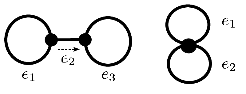
There are two operations on graphs that do not change the set of prime cycles. The first one is adding or removing a vertex of degree two on any edge. The second one is adding or removing an edge with a vertex of degree one. With these two operations, all graphs that have two linearly independent cycles are reduced to three types of graphs. The first type is in figure 7. The other types are in figure 8.
Refer to caption
Figure 8: Two other types of graphs.
Refer to caption
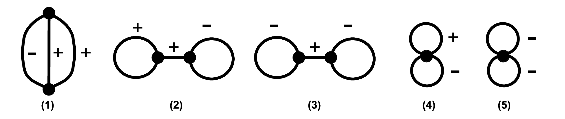
Figure 9: List of interaction types.

Up to equivalence of interactions, all types of signs of two body interactions are listed in figure 9 except for the attractive case. We check the uniqueness for each case in order.

Case (1): Proved in Example 2.

Case (2): In this case,

ℬ​ℳ=[βe1000βe10βe200βe2000βe3βe3000000βe1βe1000βe200βe20βe3000βe3],\mathcal{B}\mathcal{M}=\left[\begin{array}[]{cccccc}{\beta}_{e_{1}}&0&0&0&{\beta}_{e_{1}}&0\\ {\beta}_{e_{2}}&0&0&{\beta}_{e_{2}}&0&0\\ 0&{\beta}_{e_{3}}&{\beta}_{e_{3}}&0&0&0\\ 0&0&0&{\beta}_{e_{1}}&{\beta}_{e_{1}}&0\\ 0&0&{\beta}_{e_{2}}&0&0&{\beta}_{e_{2}}\\ 0&{\beta}_{e_{3}}&0&0&0&{\beta}_{e_{3}}\end{array}\right],

where rows and columns are labeled by e1,e2,e3,e1¯,e2¯e_{1},e_{2},e_{3},\bar{e_{1}},\bar{e_{2}} and e3¯\bar{e_{3}}. Then the determinant is

det(I−ℬ​ℳ)=(1−βe1)​(1−βe3)​(1−βe1−βe3+βe1​βe3−4​βe1​βe22​βe3).\det(I-\mathcal{B}\mathcal{M})=(1-{\beta}_{e_{1}})(1-{\beta}_{e_{3}})(1-{\beta}_{e_{1}}-{\beta}_{e_{3}}+{\beta}_{e_{1}}{\beta}_{e_{3}}-4{\beta}_{e_{1}}{\beta}_{e_{2}}^{2}{\beta}_{e_{3}}). (48)

This is positive when 0≤βe1,βe2<10\leq\beta_{e_{1}},{\beta}_{e_{2}}<1 and −1<βe3≤0-1<\beta_{e_{3}}\leq 0.

Case (3): The determinant (48) is also positive when 0≤βe2<10\leq{\beta}_{e_{2}}<1 and −1<βe1,βe3≤0-1<\beta_{e_{1}},\beta_{e_{3}}\leq 0.

Case (4): In this case,

ℬ​ℳ=[βe1βe10βe1βe2βe2βe200βe1βe1βe1βe20βe2βe2],\mathcal{B}\mathcal{M}=\left[\begin{array}[]{cccc}{\beta}_{e_{1}}&{\beta}_{e_{1}}&0&{\beta}_{e_{1}}\\ {\beta}_{e_{2}}&{\beta}_{e_{2}}&{\beta}_{e_{2}}&0\\ 0&{\beta}_{e_{1}}&{\beta}_{e_{1}}&{\beta}_{e_{1}}\\ {\beta}_{e_{2}}&0&{\beta}_{e_{2}}&{\beta}_{e_{2}}\end{array}\right],

where rows and columns are labeled by e1,e2,e1¯e_{1},e_{2},\bar{e_{1}} and e2¯\bar{e_{2}}. Then we have

det(I−ℬ​ℳ)=(1−βe1)​(1−βe2)​(1−βe1−βe2−3​βe1​βe2).\det(I-\mathcal{B}\mathcal{M})=(1-{\beta}_{e_{1}})(1-{\beta}_{e_{2}})(1-{\beta}_{e_{1}}-{\beta}_{e_{2}}-3{\beta}_{e_{1}}{\beta}_{e_{2}}). (49)

This is positive when 0≤βe1<10\leq{\beta}_{e_{1}}<1 and −1<βe2≤0-1<\beta_{e_{2}}\leq 0.

Case (5): The determinant (49) is positive when −1<βe1,βe2≤0-1<\beta_{e_{1}},\beta_{e_{2}}\leq 0.