Cup-length estimates for leaf-wise intersections

Let $(M,\omega)$ be a symplectic manifold and $\Sigma\subset M$ be a hypersurface. Then $\Sigma$ is foliated by the characteristic foliation induced by the line bundle $\ker\omega|_{\Sigma}\to\Sigma$. We denote by $L_{x}$ the leaf through $x\in\Sigma$. Let $\psi\in\mathrm{Ham}(M)$ be a Hamiltonian diffeomorphisms. Then a leaf-wise intersection is a point $x\in\Sigma$ with the property that $\psi(x)\in L_{x}$.

Let $(M,\omega)$ be a symplectic manifold and $f\in C^{\infty}(M)$ an autonomous Hamiltonian function. Since energy is preserved the hypersurface $\Sigma:=f^{-1}(0)$ is invariant under the Hamiltonian flow $\phi_{f}^{t}$ of $f$. The Hamiltonian flow $\phi_{f}^{t}$ is generated by the Hamiltonian vector field $X_{f}$ which is uniquely defined by the equation $\omega(X_{f},\cdot)=df$. If $0$ is a regular value of $f$ the hypersurface is a coisotropic submanifold which is foliated by 1-dimensional isotropic leaves, see [MS98, Section 3.3]. If we denote by $L_{x}$ the leaf through $x\in\Sigma$ we have the equality

Given a time-dependent Hamiltonian function $H:[0,1]\times M\longrightarrow\mathbb{R}$ with Hamiltonian flow $\phi_{H}^{t}$ we are interested in points $x\in\Sigma$ with the property

This notion was introduced and studied by Moser in [Mos78]. Such points are called leaf-wise intersections. We recall some notions from [AF10a].

Let $(M,\omega=d\lambda)$ be an exact symplectic manifold. Then for a Moser pair $\mathfrak{M}=(F,H)$ the perturbed Rabinowitz action functional is defined by

where $\mathscr{L}_{M}:=C^{\infty}(S^{1},M)$. A critical point $(v,\eta)$ of $\mathcal{A}^{\mathfrak{M}}$ is a solution of

In [AF10a] it is proved that critical points of $\mathcal{A}^{\mathfrak{M}}$ give rise to leaf-wise intersections.

In [CF09] Cieliebak and Frauenfelder construct a Floer homology for the unperturbed Rabinowitz action functional. This has been extended to the perturbed case by the first author and Frauenfelder in [AF10a]. The corresponding Floer equation for maps $u:\mathbb{R}\times S^{1}\to M$ and $\eta:\mathbb{R}\to\mathbb{R}$ is

Here $J$ is a smooth $(s,t)$-dependent family of compatible almost complex structures and $H_{s}:S^{1}\times M\longrightarrow\mathbb{R}$ is a smooth $s$-dependent family of functions. Counting solutions of the $s$-independent equation modulo $\mathbb{R}$-action defines the boundary operator in Rabinowitz Floer homology. In this paper we do not need the full machinery of Rabinowitz Floer homology.

We set $w=(u,\eta)$ for solutions of (2.6). We will think of $w$ also as a map $w:\mathbb{R}\longrightarrow\mathscr{L}_{M}\times\mathbb{R}$.

The following has been established in [AF10a].

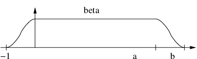
Let $k\geq 1$ be a natural number. We choose a smooth family of functions $\beta_{R}\in C^{\infty}(\mathbb{R},[0,1])$ satisfying

1. (1)

   for $R\geq 1$: $\beta_{R}^{\prime}(s)\cdot s\leq 0$ for all $s\in\mathbb{R}$, $\beta_{R}(s)=1$ for $s\in[0,(k+1)R]$, and $\beta_{R}(s)=0$ for $s\leq-1$ and $s\geq(k+1)R+1$,

2. (2)

   for $R\leq 1$: $\beta_{R}(s)\leq R$ for all $s\in\mathbb{R}$ and $\mathrm{supp}\beta_{R}\subset[-1,k+2]$,

3. (3)

   $\lim_{R\to\infty}\beta_{R}(s)=:\beta_{\infty}^{+}(s)$ and $\lim_{R\to\infty}\beta_{R}(s+(k+1)R)=:\beta_{\infty}^{-}(s)$ exists, where the limit is taken with respect to the $C^{\infty}_{loc}$ topology.

We fix a Hamiltonian function $H:[0,1]\times M\to\mathbb{R}$ with $H(t,\cdot)=0$ for all $t\in[\tfrac{1}{2},1]$ and set $K_{R}(s,t,x):=\beta_{R}(s)H(t,x)$ and

For every $R\geq 0$ we define

and

see figure 2.

We fix a natural number $k\geq 1$. The moduli space $\mathcal{M}(R)$ carries an evaluation map

For $R=0$ the evaluation map is under the identification $\mathcal{M}(0)\cong\Sigma$ the diagonal embedding $\Sigma\hookrightarrow\Delta_{\Sigma}\subset M^{k}$. Similarly, $\mathcal{M}[0,R]$ has an evaluation map $\mathrm{EV}(r,w):=\mathrm{ev}_{r}(w)$ to $M^{k}$.

Next, we define a Morse theoretic realization of the cohomology operation

where $\iota:\Sigma\hookrightarrow M$ is the inclusion map.

For that we choose Morse functions $f_{1},\ldots,f_{k}:M\to\mathbb{R}$ and $f_{*}:\Sigma\to\mathbb{R}$ and Riemannian metrics $g_{1},\ldots,g_{k},g_{*}$. We set for critical points $x_{j}\in\mathrm{Crit}(f_{j})$ and $x_{*}^{\pm}\in\mathrm{Crit}(f_{*})$

see figure 3. In particular, $\mathcal{M}(0,x_{1},\ldots,x_{k},x_{*}^{\pm})=\emptyset$ unless $\bigcap W^{s}(x_{i},f_{i})\cap\Sigma\neq\emptyset$. We denote by $\mathrm{CM}^{*}(f)$ the Morse chain complex associated to a Morse-Smale pair $(f,g)$.

Since the moduli space $\mathcal{M}(R)$ is the zero-set of a Fredholm section $\mathcal{F}(R)$ and since $\mathcal{M}(R)$ is compact we can choose an arbitrarily small abstract perturbation of the Fredholm section $\mathcal{F}(R)$ such that the zero-set $\widetilde{\mathcal{M}}(R)$ of the perturbed Fredholm section $\widetilde{\mathcal{F}}(R)$ is a smooth compact finite-dimensional manifold. Since $\mathcal{M}(R)$ is already transverse for sufficiently small $R$ we can arrange that $\widetilde{\mathcal{M}}(R)=\mathcal{M}(R)$ for small $R$. We point out that $\mathcal{M}[0,R]$ has a natural projection to $[0,R]$. The same abstract perturbation procedure gives rise to smooth perturbed moduli spaces $\widetilde{\mathcal{M}}[0,R]$ where the perturbation can be chosen with fixed ends, i.e., the fibers over $0$ resp. $R$ are $\mathcal{M}(0)$ resp.  $\widetilde{\mathcal{M}}(R)$. The perturbed moduli space $\widetilde{\mathcal{M}}(R)$ resp. $\widetilde{\mathcal{M}}[0,R]$ still carries an evaluation map $\widetilde{\mathrm{ev}}(R):\widetilde{\mathcal{M}}(R)\to M^{k}$ resp. $\widetilde{\mathrm{EV}}:\widetilde{\mathcal{M}}[0,R]\to M^{k}$.

For Morse functions $f_{1},\ldots,f_{k}:M\to\mathbb{R}$ and $f_{*}:\Sigma\to\mathbb{R}$, Riemannian metrics $g_{1},\ldots,g_{k},g_{*}$, and critical points $x_{j}\in\mathrm{Crit}(f_{j})$ and $x_{*}^{\pm}\in\mathrm{Crit}(f_{*})$ we set

see figure 4.

We assume that $\psi$ has only finitely many leaf-wise intersections since otherwise we are done. We set $k:=\mathrm{cl}(\Sigma,M)$. It has been proved in [AF10a] that $\nu_{\text{leaf}}(\psi)\geq 1$ if $||\psi||<\wp(\Sigma,\alpha)$. Thus, we may assume that $k\geq 1$. We choose a Hamiltonian $H:[0,1]\times M\to\mathbb{R}$ with $H(t,\cdot)=0$ for $t\in[\tfrac{1}{2},1]$ such that $\phi_{H}^{1}=\psi$. Let $\mathcal{LI}\subset\Sigma$ be the set of leaf-wise intersections of $\psi$.

We choose Morse functions $f_{1},\ldots,f_{k}$ and Riemannian metrics $g_{1},\ldots,g_{k}$ on $M$ and $f_{*}$, $g_{*}$ on $\Sigma$ with the following properties

1. (1)

   For $x_{i}\in\mathrm{Crit}(f_{i})$ with Morse index $\mu_{\mathrm{Morse}}(x_{i},f_{i})\neq 0$ we have $W^{s}(x_{i},f_{i})\cap\mathcal{LI}=\emptyset$.

2. (2)

   For all $n\in\mathbb{N}$ the evaluation maps $\widetilde{\mathrm{ev}}_{n}:\widetilde{\mathcal{M}}(n)\to M^{k}$ are transverse to the products of stable manifolds of the $(f_{i},g_{i})$.

3. (3)

   For all $n\in\mathbb{N}$ the evaluation maps at $\pm\infty$ are transverse to all stable and unstable manifolds of $(f_{*},g_{*})$.

The second and third property holds for a fixed $n$ for a Baire set of Morse functions and Riemannian metrics as explained in the proofs of Propositions 4.2 and 4.4. Intersecting these Baire sets over $n\in\mathbb{N}$ we see (2) and (3) is a generic property. Avoiding finitely many unstable manifolds not of top dimension is clearly also a generic condition.

By definition of $k$ we find cohomology classes $a_{1},\ldots,a_{k}\in\mathrm{H}^{\geq 1}(M)$ with $\iota^{*}(a_{1}\cup\ldots\cup a_{k})\neq 0\in\mathrm{H}^{*}(\Sigma)$. Thus, the cohomology operation $\Theta$, see equation (4.2), is non-zero. According to Propositions 4.2 and 4.4 the cohomology operations $\theta_{R}$ then have to be non-zero for all $R\geq 0$. Thus, we can find critical points $x_{i}\in\mathrm{Crit}(f_{i})$ with Morse index $\mu_{\mathrm{Morse}}(x_{i},f_{i})\neq 0$ and $x_{*}^{\pm}\in\mathrm{Crit}(f_{*})$ such that for all $n\in\mathbb{N}$ the moduli spaces

In fact, the choice of $x_{i}\in\mathrm{Crit}(f_{i})$ will depend on $n$ in general. For notational convenience we suppress the $n$. In fact, there exists a subsequence $n_{k}$ for which we can choose $x_{i}$ fixed. We conclude

If the unperturbed moduli space $\mathcal{M}(n)$, see equation (3.2), were empty then for sufficiently small perturbations of the Fredholm section also the moduli space $\widetilde{\mathcal{M}}(n)$ would be empty. Indeed, if $\mathcal{M}(n)=\emptyset$ then the corresponding Fredholm section is transverse. Since $\mathcal{M}(n)$ is compact a sufficiently small perturbation of the Fredholm section remains empty and thus transverse. Therefore, we conclude that

Now we can choose a sequence $w_{n}\in\mathcal{M}(n)$, that is, $w_{n}$ solves equation (2.8) with Hamiltonian perturbation $\beta_{n}(s)H(t,x)$. Since $\widetilde{\mathcal{M}}(n)\cap_{\widetilde{\mathrm{ev}}_{n}}\big(W^{s}(x_{1},f_{1})\times\ldots\times W^{s}(x_{k},f_{k})\big)\neq\emptyset$ and all evaluation maps are transverse a similar argument as above allows us to conclude that

By Lemma 3.1 the action $\mathcal{A}^{\mathfrak{M}_{n}}(w_{n}(s))$ is uniformly bounded and we can apply Theorem 2.10. We consider the following sequences

For $j=1,\ldots,k$ these sequences converge (after choosing a subsequence) to solutions $\varpi^{j}=(u^{j},\eta^{j}):\mathbb{R}\to\mathscr{L}_{M}\times\mathbb{R}$ of

of energy

The sequence $w_{n}(s)$ converges to a solution $\varpi^{0}=(u^{0},\eta^{0})$ of

References

• [AF08] P. Albers and U. Frauenfelder, Infinitely many leaf-wise intersections on cotangent bundles, 2008, arXiv:0812.4426.
• [AF10a] by same author, Leaf-wise intersections and Rabinowitz Floer homology, J. Topol. Anal. 2 (2010), no. 1, 77–98.
• [AF10b] by same author, On a Theorem by Ekeland-Hofer, 2010, arXiv:1001.3386, to appear in Israel Journal of Mathematics.
• [AF10c] by same author, Spectral invariants in Rabinowitz Floer homology and global Hamiltonian perturbations, 2010, arXiv:1001.2920.
• [AM09] P. Albers and M. McLean, Non-displaceable contact embeddings and infinitely many leaf-wise intersections, 2009, arXiv:0904.3564, to appear in Journal of Symplectic Geometry.
• [Ban80] A. Banyaga, On fixed points of symplectic maps, Invent. Math. 56 (1980), no. 3, 215–229.
• [CF09] K. Cieliebak and U. Frauenfelder, A Floer homology for exact contact embeddings, Pacific J. Math. 293 (2009), no. 2, 251–316.
• [Dra08] D. L. Dragnev, Symplectic rigidity, symplectic fixed points, and global perturbations of Hamiltonian systems, Comm. Pure Appl. Math. 61 (2008), no. 3, 346–370.
• [EH89] I. Ekeland and H. Hofer, Two symplectic fixed-point theorems with applications to Hamiltonian dynamics, J. Math. Pures Appl. (9) 68 (1989), no. 4, 467–489 (1990).
• [Flo89] A. Floer, Cuplength estimates on Lagrangian intersections, Comm. Pure Appl. Math. 42 (1989), no. 4, 335–356.
• [Gin07] V. L. Ginzburg, Coisotropic intersections, Duke Math. J. 140 (2007), no. 1, 111–163.
• [Gür09] B. Gürel, Leafwise Coisotropic Intersections, Int. Math. Res. Not. (2009), article ID rnp 164.
• [Hof88] H. Hofer, Lusternik-Schnirelman-theory for Lagrangian intersections, Ann. Inst. H. Poincaré Anal. Non Linéaire 5 (1988), no. 5, 465–499.
• [Hof90] by same author, On the topological properties of symplectic maps, Proc. Roy. Soc. Edinburgh Sect. A 115 (1990), no. 1-2, 25–38.
• [Kan09] J. Kang, Existence of leafwise intersection points in the unrestricted case, 2009, arXiv:0910.2369.
• [Liu05] C.-G. Liu, Cup-length estimate for Lagrangian intersections, J. Differential Equations 209 (2005), no. 1, 57–76.
• [Mer10] W. Merry, On the Rabinowitz Floer homology of twisted cotangent bundles, 2010, arXiv:1002.0162.
• [Mos78] J. Moser, A fixed point theorem in symplectic geometry, Acta Math. 141 (1978), no. 1–2, 17–34.
• [MS98] D. McDuff and D. A. Salamon, Introduction to symplectic topology, second ed., Oxford Mathematical Monographs, The Clarendon Press Oxford University Press, New York, 1998.
• [Sch93] M. Schwarz, Morse homology, Progress in Mathematics, vol. 111, Birkhäuser Verlag, Basel, 1993.
• [Sch98] by same author, A quantum cup-length estimate for symplectic fixed points, Invent. Math. 133 (1998), no. 2, 353–397.
• [Zil08] F. Ziltener, Coisotropic Submanifolds, Leafwise Fixed Points, and Presymplectic Embeddings, 2008, arXiv:0811.3715, to appear in Journal of Symplectic Geometry.