QUANTUM SPIN CHAINS AT FINITE TEMPERATURES

Let ${\cal H}$ be the Hamiltonian of a 1D quantum system of size $L$ and $V$ its space of states. Our goal is to calculate the thermal expectation value of any physical quantity ${\cal O}$ at temperature $T(=1/\beta)$¹¹ 1 The Boltzmann constant $k_{B}$ is set to be unity in this report. in the limit $L\rightarrow\infty$,

Here $E_{j}$ stands for an eigenvalue of ${\cal H}$.

The definition requires both diagonalization and summation. Below we shall show how we can avoid the latter within the framework of QTM.

To be concrete, we specify a Hamiltonian. As a prototypical integrable lattice system we choose the 1D spin $\frac{1}{2}$ XXZ model,

where the $\sigma^{a}\,(a=x,y,z)$ are the Pauli matrices. The periodic boundary conditions (PBCs) imply $\sigma^{a}_{L+1}=\sigma^{a}_{1}$. The anisotropy is parameterized as $\Delta=\cos\gamma$. The Hamiltonian acts on “the physical space” $V_{\rm phys}:=\bigotimes_{j=1}^{L}V_{j}$ where $V_{j}$ denotes the $j$th copy of a two-dimensional vector space $c_{1}{\bf e}_{+}+c_{2}{\bf e}_{-}$. The trace in (1) must be performed over $V_{\rm phys}$. By definition the “Hamiltonian density” $\hat{h}_{j,j+1}$ is the $j$th summand in the first sum in (2). It acts non-trivially only on $V_{j}\otimes V_{j+1}$.

The above Hamiltonian is integrable in the following sense. Let $R(u,v)$ be the $U_{q}(\widehat{\mathfrak{sl}_{2}})$ $R$ matrix[6],

depending on the spectral parameters (or rapidities) $u,v\in\mathbb{C}$. We define $E^{\alpha}_{\beta}$ s.t. $(E^{\alpha}_{\beta})_{i,j}=\delta_{\alpha,i}\delta_{\beta,j}$. Then the matrix elements $R_{\beta\delta}^{\alpha\gamma}$ can be read off from

The index $1(2)$ refers to ${\bf e}_{+}({\bf e}_{-})$. See fig. 1 for a graphic representation.

We put arrows, to distinguish the $R$ matrix from other $R$ matrices appearing below. The reader should not confuse them with physical variables.

By $R_{j,j+1}(u,v)$ we mean the $R$ matrix acting non-trivially only on the tensor product $V_{j}(u)\otimes V_{j+1}(v)$ of $U_{q}(\widehat{\mathfrak{sl}_{2}})$ modules. We also introduce the intertwiner $R^{\vee}_{j,j+1}(u,v)=P_{j,j+1}R_{j,j+1}(u,v)$, where $P:V_{j}(u)\otimes V_{j+1}(v)\rightarrow V_{j+1}(v)\otimes V_{j}(u)$. Then, with $q={\rm e}^{i\gamma}$, we have the expansion

where $\hat{h^{\prime}}_{j,j+1}:=iJ\sin\gamma(\sigma^{z}_{j}-\sigma^{z}_{j+1})$. We introduce the row-to-row (RTR) transfer matrix $T_{\rm RTR}(u)\in{\rm End}(V_{\rm phys})$,

With the lattice translation operator ${\rm e}^{iP}$, shifting the state by one site, we obtain the Baxter-Lüscher formula[3]

Note that the $\hat{h^{\prime}}_{j,j+1}$ terms cancel due to the PBCs. The huge symmetry $U_{q}(\widehat{\mathfrak{sl}_{2}})$ is at the bottom of the integrability of the Hamiltonian.

We first present the formula for the free energy per site in the QTM formalism. A supplemental discussion will be given in subsequent sections.

We introduce the transposed $R$ matrix $R^{t}_{j,k}(u,v)$[7] by $(R^{t})^{\alpha\gamma}_{\beta\delta}(u,v)=R^{\delta\alpha}_{\gamma\beta}(v,u).$ See fig. 2.

The QTM does not act on $V_{\rm phys}$ but on a fictitious space $V_{\rm Trotter}=V_{1}(u)\otimes V_{2}(-u)\otimes\cdots V_{N-1}(u)\otimes V_{N}(-u)$. The fictitious system size $N$ is often referred to as the Trotter number. The parameter $u$ is fixed to be

In its most sophisticated version, the QTM is explicitly defined by [7],

The new parameter $x$ will later play the role of a spectral parameter. The factor $i$ is introduced for convenience.

We are now in a position to write down the formula for the free energy per site in the thermodynamic limit, $f=-\lim_{L\rightarrow\infty}\frac{T}{L}\ln Z_{{\rm 1D}}(\beta)$.

The limit $N\rightarrow\infty$ is referred to as the Trotter limit. As was announced earlier, eq. (6) expresses $f$ without recourse to any summation. We also note that $\ln\Lambda_{0}$ itself is already intensive, which may reflect the size dependent interaction of the system.

The quantitative analysis of (6) is most efficiently performed by means of the NLIE. Having in mind the examples, from now on we are considering only for $J=\frac{1}{4},\gamma\rightarrow 0$ and $u=-\frac{\beta}{N}$, consequently. Let $\mathfrak{a}$ be the unique solution to the NLIE²² 2 To be precise, there are, in general, several equivalent versions of NLIEs. We present one of these below.

Here the contour ${\cal C}$ is a closed narrow loop which encircles all “Bethe roots”. We added a Zeeman term $\frac{h}{2}\sum_{j}\sigma^{z}_{j}$ to the Hamiltonian so that ${\rm diag}(\exp(-\frac{\beta h}{2}),\exp(\frac{\beta h}{2}))$ is inserted in the trace in (5). Then we have the following

Note that the NLIE (7) and the expression for $f$ in (8) are independent of $N$. The extension to arbitrary $J,\gamma$ is straightforward.

Below we shall comment on the derivation of the formula. By presenting supplementary arguments, we wish to convince the reader that the above formalism, seemingly complicated, is actually necessary and efficient for many purposes. Hereafter we set again $h=0$ for simplicity.

We define a rotated R matrix $\widetilde{R}(u,v)$ by $\widetilde{R}^{\alpha\gamma}_{\beta\delta}(u,v)=R^{\gamma\beta}_{\delta\alpha}(v,u)$ (fig. 3). Then we introduce a rotated transfer matrix $\widetilde{T}_{\rm RTR}(u)\in{\rm End}(V_{\rm phys})$ by

Analogous to (4) $\widetilde{T}_{\rm RTR}(u)={\rm e}^{-iP}\bigl(1+u\,{\cal H}+O(u^{2})\bigr).$

We thus obtain an important identity,

where $T_{\rm double}(u):=T_{\rm RTR}(u)\widetilde{T}_{\rm RTR}(u)$. The rhs of (9) can be interpreted as a partition function of a 2D classical system defined on $N\times L$ sites (fig. 4),

This equivalence lies in the heart of the QTM formalism. The expression (9) itself, however, is of no direct use for the actual evaluation of physical quantities for the following reason.

Let the eigenvalue spectrum of $T_{\rm RTR}(u)$ be $\lambda_{0}(x)>\lambda_{1}(x)\geq\lambda_{2}(x)\geq\cdots$. We introduced $x=i^{-1}(u+1)$ for technical reasons. It is easy to see that $\widetilde{T}_{\rm RTR}(u)$ has the same spectrum. Thus,

The eigenvalue $\lambda_{j}(x)$ is characterized by its zeros $\pm\theta_{a}\,(a=1,2,\dots)$ on the real axis (holes). We know numerically that for low excitations, $\theta_{a}\sim\ln L$ and also that $\lambda_{j}(x)$ is analytic and nonzero in the strip $|\Im{\rm m}x|\leq 1$ except at $\pm\theta_{a}$. Let us introduce an analytic and nonzero function near the real axis, ${\lambda}^{\sharp}_{j}$, by $\lambda_{j}(x)=\prod_{a}\tgh\frac{\pi}{4}(x-\theta_{a})\tgh\frac{\pi}{4}(x+\theta_{a}){\lambda}^{\sharp}_{j}(x)$. It approximately satisfies the inversion relation for $L\gg 1$,

where $\phi(x)$ is a known function common to any $j$. Thus, we simply have

For very low excitations, we take a single pair of holes, substitute $\theta_{a}\sim\frac{2}{\pi}\ln\frac{2\pi L}{\Delta_{j}}$ and take the large $L$ limit. Then we arrive at the estimate ($u\sim 0$)

For a usual 2D classical system we can consider an infinitely long cylinder and take $\frac{N}{L}\gg 1$. We thus have to take into account only the first term on the rhs in (10). By contrast, the spectral parameter depends on the fictitious system size $u=-\frac{\beta}{N}$ in the present case. Therefore, as long as $T\neq 0$, we have

Fig. 5 presents numerical evidence for the above argument. The left figure shows the histogram of the distribution of $|\lambda_{j}/\lambda_{0}|$ for $q=1,L=10,u=-0.01$ in the sector with vanishing magnetization. One clearly sees that the maximum of the distribution lies near $|\lambda_{j}/\lambda_{0}|\sim 1$. The right figure magnifies the region near $|\lambda_{j}/\lambda_{0}|\sim 1$. The maximum is located around $|\lambda_{j}/\lambda_{0}|\sim 0.96$. We believe that, with increasing $L$, the peak moves towards $|\lambda_{j}/\lambda_{0}|\sim 1$. These findings are consistent with (12).

Hence, we conclude that infinitely many terms of the sum in the rhs of (10) contribute non-trivially, and eq. (9) is of no practical use.

A crucial observation was made in reference[4]. We start from the same two-dimensional classical model in fig. 4. We consider, however, the transfer matrix propagating in horizontal direction, that is, $T^{\prime}_{\rm QTM}(u)$. Equivalently, one can rotate the system by 90^∘. Then we define a transfer matrix propagating in vertical direction, $T_{\rm QTM}(u)$ (see fig. 6). The latter is more convenient for our formulation.

The partition function is then given by,

Let the eigenvalue spectrum of $T_{\rm QTM}(u)$ be $\Lambda_{0}(u)>\Lambda_{1}(u)\geq\Lambda_{2}(u)\geq\cdots$. Then we have an expansion similar to (10)

Our physical interest is in the free energy per site $f$ in the thermodynamic limit $L\rightarrow\infty$.

We supplement an argument which claims that the second term in the second line in (15) is negligible for $L\rightarrow\infty$. The previous argument, using the inversion relation (11) can not be applied directly as the spectral parameter $u$ is already fixed as $-\frac{\beta}{N}$ in the present problem.

We introduce a slight generalization, a commuting QTM $T_{QTM}(x,u)$, by assigning the parameter $ix$ in “horizontal” direction[10]. The substitution $x=0$ recovers the previous results. The precise definition is shown in (5). Hereafter we drop the $u$ dependence as it is always $-\frac{\beta}{N}$. Let ${\cal T}_{\rm QTM}(x)$ be the corresponding monodromy matrix. Then it is easy to see that monodromy matrices are intertwined by the same $R$ matrix as in the RTR case,

This immediately proves the commutativity of ${T}_{\rm QTM}(x)$ with different $x$’s.

The most important consequence of introducing $x$ is that we have the inversion relation in this new “coordinate”,

where we set again $\Lambda_{j}(x)=\prod_{a}\tgh\frac{\pi}{4}(x-\theta_{a})\tgh\frac{\pi}{4}(x+\theta_{a}){\Lambda}^{\sharp}_{j}(x)$. Note that ${\Lambda}^{\sharp}_{j}(x)$ also depends on the “old” spectral parameter $u$, which is set to be $-\frac{\beta}{N}$ on both sides. The known function $\psi$ is again independent of $j$. The analysis of the Bethe ansatz equation associated to the QTM implies that $\theta_{a}\sim\frac{2}{\pi}\ln\frac{4\beta}{\Delta_{j}}$ for large $\beta$. Then, proceeding as before, we obtain,

The diagonalization for fixed $N$ clearly shows the gap between the eigenvalues, which is consistent with the above argument. Thus, at any finite temperature, the second term in (15) is negligible for $L\rightarrow\infty$. We then conclude that the formula (6) is valid.

Although we made use of the integrability of the model in the above argument, the validity of the formula is actually independent of it. See the proof in reference[4].

Thanks to (16), one can apply the machinery of the quantum inverse scattering method, devised originally for the diagonalization of $T_{\rm RTR}$, to the diagonalization of $T_{\rm QTM}$. We skip the derivation and present only results relevant for our subsequent discussion³³ 3 A technical remark: the vacuum is conveniently chosen $(+,-,+,-,\cdots)$.. We fix $N$ for a while. Then the eigenvalue of $T_{\rm QTM}$ is given by

The different sets of Bethe roots $\{x_{j}\}$ correspond to the different eigenvalues. They satisfy the Bethe ansatz equation (BAE),

For the largest eigenvalue the number of roots $m$ equals $\frac{N}{2}$.

To evaluate $f$ via (6) we need the largest $\Lambda^{(N)}$ for $N\rightarrow\infty$. This means we must deal with infinitely many roots in the limit, which resembles the situation encountered in the evaluation of the free energy in the thermodynamic limit of a classical 2D model by means of the RTR transfer matrix. Still, we would like to comment on the qualitative difference in the root distribution between such “standard” case and the problem under discussion.

Fig. 7 shows the distribution of the positive half of BAE roots for the largest eigenvalue of $T_{\rm RTR}$ (left) and $T_{\rm QTM}$ (right) for various system sizes.

The distribution of RTR roots behaves smoothly for large system size. The limiting shape of the distribution (the root density function) is a smooth function satisfying a linear integral equation. For $T_{\rm QTM}$, on the other hand, a few large roots remain isolated at almost the same positions as $N$ increases, while close to the origin more and more Bethe roots cluster.

Let us describe this in detail. Using the NLIE technique, we can derive an approximate BAE equation (see the discussion after (25)),

The hole $\theta_{a}$ corresponds to the branch cut integer $I_{\rm max}=\frac{N}{4}-\frac{1}{2}$, and this implies $\theta_{a}\sim\frac{1}{\pi}\ln\beta$ for $\beta\gg 1$, which was used in the last subsection.

Near the origin, we set $x_{j}=\frac{\beta}{N}\widehat{x}_{j}$, and obtain the approximate distribution of $\widehat{x}_{j}$ as an algebraic function,

This differs from the usual root density function which decays exponentially as $|x|\rightarrow\infty$. In the original variable, if we take the Trotter limit naively,

Namely the distribution of the BAE roots for $T_{\rm QTM}$ is singular in the Trotter limit. We thus conclude that the usual root density method may not be applicable, and we have to devise a different tool.

One must intrinsically deal with a finite size system with coupling constant $u$ depending on the Trotter size, and then take the Trotter limit. Such an attempt was executed first numerically[8] by extrapolation in $N$. The analytic low temperature expansion was performed[9] based on the Wiener-Hopf method. Below we shall present the most sophisticated approach which utilizes the commuting QTM in a most efficient manner[7].

The introduction of the new spectral parameter $x$ plays a fundamental role. Instead of dealing with the BAE roots directly, we make use of the analyticity of specially chosen auxiliary functions in the complex $x$ plane.

There are various approaches. One of them is to introduce the fusion hierarchy of the QTM, which contains the original $T_{\rm QTM}$ as $T_{1}$. In place of the BAE one uses the functional relations among fusion transfer matrices,

Here $\psi_{1}$ is nothing but $\psi$ in the inversion relation (17), where the small term $T_{0}T_{2}/\psi_{1}$ was neglected. As $\{T_{m}\}$ constitutes a commuting family, the same relation holds among the eigenvalues. We thus use the same symbol $T_{m}$ for the eigenvalue. After a change of variables, $y_{m}(x)=T_{m-1}(x)T_{m+1}(x)/\psi_{m}(x)$, one can transform the algebraic equations into integral equations under certain assumptions on the analyticity of $y_{m}$. The resultant equations coincide with the Thermodynamic Bethe Ansatz equations[10, 11]. The string hypothesis is thus replaced by an assumption on the analyticity of $y_{m}$. The coupled set of equations may fix the values of $T_{1}(x)$. Then $\Lambda_{0}=T_{1}(0)$ yields the free energy per site $f$. A technical problem in this approach is that we must deal with an infinite number of $y_{m}$ functions, which requires a truncation of the equations in an approximate manner.

Below we shall discuss another approach originally devised in the context of the evaluation of finite size corrections[12]. We define the auxiliary function $\mathfrak{a}_{N}(x)$ by the ratio of the two terms in $\Lambda^{(N)}(x)$ (18),

The suffix $N$ is introduced to recall that we are fixing $N$ finite here. The BAE (19) is equivalent to the condition

We also note that $\lim_{|x|\rightarrow\infty}\mathfrak{a}_{N}(x)=1$ by construction.

We then adopt the following assumptions for the analytic properties of $\mathfrak{A}_{N}(x)$ corresponding to the largest eigenvalue. They are supported by numerical calculations.

1. 1.

   There are $\frac{N}{2}$ simple zeros of $\mathfrak{A}_{N}(x)$ on the real axis. They coincide with the BAE roots. There are additional zeros, sufficiently far away from the real axis, so that ${\cal C}$ does not include them inside.

2. 2.

   The only pole of $\mathfrak{A}_{N}(x)$ in $\Im x\in[-1,1]$ is located at $x=iu$ and is of order $\frac{N}{2}$.

Once these assumptions are granted, one immediately derives the following NLIE,

The largest eigenvalue $\Lambda$ can be similarly represented by

Note that only the driving term in (23) depends on $N$. We can thus take the Trotter limit easily, with $\mathfrak{a}:=\lim_{N\rightarrow\infty}\mathfrak{a}_{N}$, and obtain the NLIE in (7) (for $h=0$). To evaluate the free energy one has to first set $x=0$, then take the Trotter limit. Or otherwise one meets a spurious divergence. Then we obtain the expression for the free energy in Theorem 2.2.

One still needs to make an effort to achieve a high numerical accuracy, especially at very low temperatures. The introduction of another pair of auxiliary functions solves this problem. We define $\bar{\mathfrak{a}}_{N},\bar{\mathfrak{A}}_{N}$ by $\bar{\mathfrak{a}}_{N}(x)=(\mathfrak{a}_{N}(x))^{-1}$, $\bar{\mathfrak{A}}_{N}(x)=1+\bar{\mathfrak{a}}_{N}(x)$.

Numerically one finds that $|\mathfrak{a}_{N}|\lessgtr 1$ for $\Im x\gtrless 0$. Thus, we use $\mathfrak{a}_{N},\mathfrak{A}_{N}$ in the upper half plane and $\bar{\mathfrak{a}}_{N},\bar{\mathfrak{A}}_{N}$ in the lower half plane. It is straightforward to rewrite (23) in the coupled form,

where $C_{+}(C_{-})$ is a straight contour slightly above (below) the real axis. In the first (second) equation we understand that $x\in C_{+}(C_{-})$. Note that the convolution terms bring only minor contributions as they are defined on those contours where the auxiliary functions are small. Therefore the main contributions come from the known functions. This enables us to perform numerics with high accuracy. We can drop the convolution terms for the lowest order approximation. Thanks to eq. (22) this leads to eq. (20).

Similarly, for the largest eigenvalue we have

We obtain the NLIE and the eigenvalue in the Trotter limit by replacing $\mathfrak{a}_{N}\rightarrow\mathfrak{a}$ etc. and

For the actual calculation, it is even better to deal with $\mathfrak{b}(x):=\mathfrak{a}(x+i)$ and $\bar{\mathfrak{b}}(x):=\bar{\mathfrak{a}}(x-i)$ so that the singularities of $\ln(1+\mathfrak{b}),\ln(1+\bar{\mathfrak{b}})$ are away from the integration contours. We omit, however, the details.

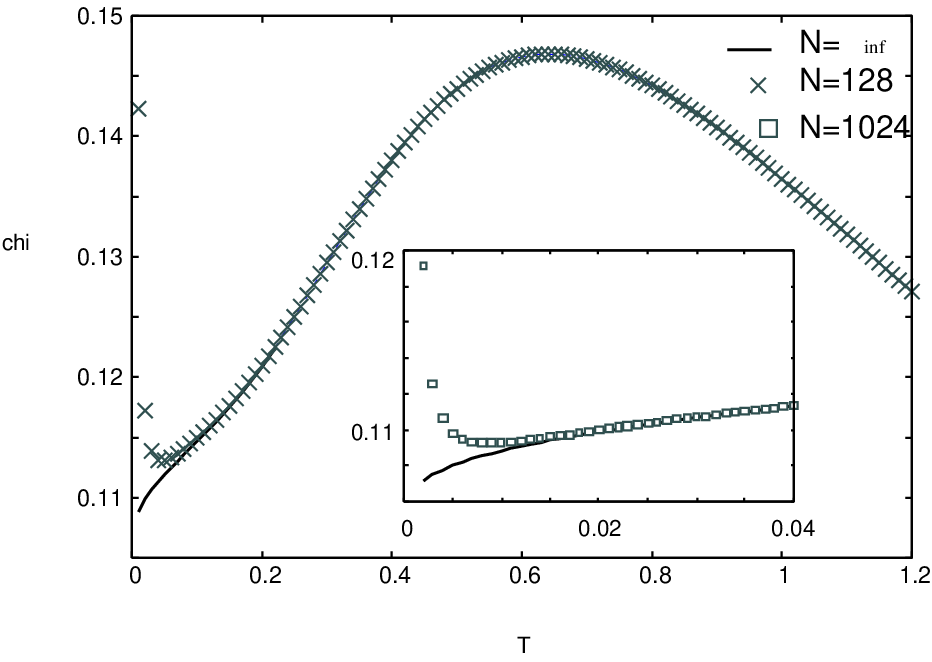
As a concrete example for the evaluation of bulk quantities we plot the susceptibility, $\chi=\partial^{2}_{h}f$, in fig. 8 (left). Note that at low temperatures the physical result in the Trotter limit (solid line) deviates from its finite Trotter number approximation.

The above approach has been successfully applied to many models of physical relevance[13, 14, 15, 16, 17, 18, 19].

The correlation length $\xi$ characterizes the decay of correlation functions at large distance, e.g.,

It is evaluated from the ratio of the largest and the second largest eigenvalues of the QTM[20, 9, 21, 22]. For the second largest eigenvalue state, our assumption (1) on $\mathfrak{A}$ is no longer valid: a pair of holes $\theta_{a}$ lies on the real axis, and they are zeros of $\mathfrak{A}$ other than Bethe roots. Nevertheless, a small modification leads to a set of equations that fixes the second largest eigenvalue. The resultant NLIE has a form similar to (25) containing, however, additional inhomogeneous terms. Fig. 8 (right) shows a plot of $\xi T$ against temperature for the XXZ model with $q={\rm e}^{i\frac{\pi}{p}}$ for $p=3,4,5$[21].

When $h\neq 0$, we have to replace $a(x),d(x)$ in (18) by ${\rm e}^{-\beta h/2}a(x)$, ${\rm e}^{\beta h/2}d(x)$. Then we add $\beta h$ $(-\frac{\beta h}{2})$ to the rhs of (23) ((24)). Also $D^{(N)}_{\pm}$ must be replaced by $D^{(N)}_{\pm}\pm\frac{\beta h}{2}$.

Before closing this section, we would like to mention another formulation of thermodynamics also based on the QTM[23]. It is described by a NLIE for $\Lambda_{j}$ directly and allows one to efficiently calculate high temperature expansions. The good numerical accuracy in the low temperature region is, however, hard to achieve. Moreover, we point out that the equation is the same for any eigenvalue. Thus, one should know a priori good initial values in order to select the convergence to the desired eigenvalue.

References

- [1] M. Gaudin, Phys. Rev. Lett. 26 (1971) 1301.
- [2] M. Takahashi and M. Suzuki, Prog. Theor. Phys. 48 (1972) 2187-2209.
- [3] R. J. Baxter, Ann. Phys. 76 (1973) 1, ibid, 25, ibid 48.
- [4] M. Suzuki, Phys. Rev. B 31 (1985) 2957-2965.
- [5] For earlier reviews on the QTM and finite size correction method, see e.g. J. Suzuki, T. Nagao and M. Wadati, Int. J. Mod. Phys. B 6 (1992) 1119-1180. A. Klümper, Lecture Notes in Phys. 645 (2004) 349-379, or the review chapters in the book by F. H. L. Essler, H. Frahm, F. Göhmann, A. Klümper and V. E. Korepin, “The One-Dimensional Hubbard Model” (Cambridge Press 2005).
- [6] M. Jimbo, Lett. Math. Phys. 10 (1985) 63-69.
- [7] A. Klümper, Z. Phys. B 91 (1993) 507-519.
- [8] T. Koma, Prog. Theor. Phys. 78 (1987) 1213-1218.
- [9] J. Suzuki, Y. Akutsu and M. Wadati, J. Phys. Soc. Jpn. 59 (1990) 2667-2680.
- [10] A. Klümper, Ann. Physik (Lpz.) 1 (1992) 540.
- [11] A. Kuniba, K. Sakai and J. Suzuki, Nucl. Phys. B 525 [FS] (1998) 597-626.
- [12] A. Klümper, M. T. Batchelor and P. A. Pearce, J. Phys. A 24 (1991) 3111-3133.
- [13] G. Jüttner and A. Klümper, Euro. Phys. Lett. 37 (1997) 335-340.
- [14] G. Jüttner, A. Klümper and J. Suzuki, Nucl. Phys. B 486 (1997) 650-574, J. Phys. A 30 (1997) 1881-1886, Nucl. Phys. B 512 (1998) 581-600, Nucl. Phys. B 522 (1998) 471-502.
- [15] J. Suzuki, Nucl. Phys. B 528 (1998) 683-700.
- [16] A. Fujii and A. Klümper, Nucl. Phys. B 546 (1999) 751-764.
- [17] J. Suzuki, J. Phys. A 32 (1999) 2341-2359.
- [18] M. Bortz and A. Klümper, Eur. Phys. J. B 40 (2004) 25-42.
- [19] J. Damerau and A. Klümper, JSTAT (2006) P12014.
- [20] M. Suzuki and M. Inoue, Prog. Theor. Phys. 78 (1987) 787.
- [21] K. Sakai, M. Shiroishi, J. Suzuki and Y. Umeno, Phys. Rev. B 60 (1999) 5186-5201.
- [22] A. Klümper, J. R. Reyes Martinez, C. Scheeren, M. Shiroishi, J. Stat. Phys. 102 (2001) 937-951.
- [23] M. Shirosihi and M. Takahashi, Phys. Rev. Lett. 89 (2002) 117201(4pp). Z. Tsuboi, J. Phys. A 37 (2004) 1747-1758.
- [24] M. Jimbo, K. Miki, T. Miwa, A. Nakayashiki, Phys. Lett. A 16 (1992) 256-263.
- [25] M. Jimbo and T. Miwa, J. Phys. A 29 (1996) 2923-2958.
- [26] N. Kitanine, J. M. Maillet and V. Terras, Nucl. Phys. B 567 (2000) 554-582. N. Kitanine, J. M. Maillet, N. A. Slavnov, V. Terras, Nucl. Phys. B 641 (2002) 487-518.
- [27] F. Göhmann, A. Klümper and A. Seel, J. Phys. A 37 (2004) 7625-7651.
- [28] F. Göhmann, N. Hasenclever and A. Seel, JSTAT (2005) P10015.
- [29] M. Bortz and F. Göhmann, Eur. Phys. J. B 46 (2005) 399-408.
- [30] Z. Tsuboi, Physica A 377 (2007) 95-101.
- [31] H. E. Boos and V. E. Korepin, J. Phys. A 34 (2001) 5311-5316. H. E. Boos, V. E. Korepin and F. A. Smirnov, Nucl. Phys. B 658 (2003) 417-439, J. Phys. A 37 (2004) 323-336.
- [32] K. Sakai, M. Shiroishi, Y. Nishiyama and M. Takahashi, Phys. Rev. E 67 (2003) 06510(R) (4pp). G. Kato, M. Shiroishi, M. Takahashi, K. Sakai, J. Phys. A 36 (2003) L337-L344. J. Sato, M. Shiroishi, M. Takahashi JSTAT (2006) P017.
- [33] H. Boos, M. Jimbo, T. Miwa, F. Smirnov, Y. Takeyama, Comm. Math. Phys. 261 (2006) 245-276, Annales Henri-Poincare 7 (2006) 1395-1428, Comm. Math. Phys 272 (2007) 263-281, Comm. Math. Phys. 286 (2009) 875-932.
- [34] H. E. Boos, F. Göhmann, A. Klümper and J. Suzuki, JSTAT 0604 (2006) P001, J. Phys. A 40 (2007) 10699-10728.
- [35] H. E. Boos, J. Damerau, F. Göhmann, A. Klümper and J. Suzuki and A. Weiße, JSTAT 0808 (2008) P08010.
- [36] K. Fabricius and B. M. McCoy, Phys. Rev. B 59 (1999) 381-386. K. Fabricius, A. Klümper and B. M. McCoy, Phys. Rev. Lett. 82 (1999) 5365-5368.
- [37] M. Jimbo, T. Miwa and F. Smirnov, J. Phys. A 42 (2009) 304018 (31pp).
- [38] H. Boos and F. Göhmann, J. Phys. A42 (2009) 315001 (27pp).