A Distributed Sequential Algorithm for Collaborative Intrusion Detection Networks

In this section, we use sequential hypothesis testing to make decisions with minimum number of feedback from the peer IDSs, [11], [12]. An IDS asks for feedback from its acquaintance list until a sufficient number of answers are collected. Let $\Omega^{i}$ denote all the possible collections of feedback in the acquaintance list to an IDS $i$ and $\omega^{i}\in\Omega^{i}$ denotes a particular collection of feedback. Let $N^{i}(\omega^{i})$ be a random variable denoting the number of feedbacks used until a decision is made. A sequential decision rule is formed by a pair $(\phi,\delta)$, where $\phi^{i}=\{\phi_{n}^{i},n\in\mathbb{N}\}$ is a stopping rule and $\delta^{i}=\{\delta_{n}^{i},n\in\mathbb{N}\}$ is the terminal decision rule. Introduce a stopping rule with $n$ feedback, $\phi^{i}_{n}:\mathcal{Y}_{n}^{i}:=\prod_{j\in\mathcal{N}_{i,n}}\mathcal{Y}_{j}\rightarrow\{0,1\}$, where $\mathcal{N}_{i,n}$ is the set of nodes an IDS $i$ asks up to time $n$. $\phi^{i}_{n}=0$ indicates that IDS $i$ needs to take more samples after $n$ rounds whereas $\phi^{i}_{n}=1$ means to stop asking for feedback and a decision can be made by the rule $\delta_{n}^{i}$. The minimum number of feedbacks is given by

$$N^{i}(\omega^{i})=\min\{n:\phi_{n}^{i}=1,n\in\mathbb{N}\}.$$

(5)

Note that $N^{i}(\omega^{i})$ is the stopping time of the decision rule. The decision rule $\delta^{i}$ is not used until $N.$ We assume that no cost has incurred when a correct decision is made while the cost of a missed intrusion is denoted by $C^{i}_{M}$ and the cost of a false alarm is denoted by $C_{F}^{i}$. In addition, we assume each feedback incurs a cost $D^{i}$. We introduce an optimal sequential rule that minimizes Bayes risk given by

$$R^{i}(\phi^{i},\delta^{i})=R(\phi^{i},\delta^{i}|H_{0})\pi_{0}^{i}+R(\phi^{i},\delta^{i}|H_{1})\pi_{1}^{i},$$

(6)

where $R(\phi^{i},\delta^{i}|H_{l}),l=0,1$, are the Bayes risks under hypotheses $H_{0}$ and $H_{1}$, respectively:

	$\displaystyle R^{i}(\phi^{i},\delta^{i}|H_{0})=C_{F}^{i}\mathbb{P}[\delta_{N}(Y_{j},j\in\mathcal{N}_{i,N})=1|H_{0}]+D^{i}\mathbb{E}[N|H_{0}],$
	$\displaystyle R^{i}(\phi^{i},\delta^{i}|H_{1})=C_{M}^{i}\mathbb{P}[\delta_{N}(Y_{j},j\in\mathcal{N}_{i,N})=0|H_{1}]+D^{i}\mathbb{E}[N|H_{1}].$

Let $V^{i}(\pi_{0}^{i})=\min_{\phi^{i},\delta^{i}}R^{i}(\phi^{i},\delta^{i})$ be the optimal value function. It is clear that when no feedback are obtained from the peers, the Bayes risks reduce to

	$\displaystyle R^{i}(\phi_{0}^{i}=1,\delta_{0}^{i}=1)$	$\displaystyle=$	$\displaystyle C_{F}^{i}\pi_{0}^{i},$		(7)
	$\displaystyle R^{i}(\phi_{0}^{i}=1,\delta_{0}^{i}=0)$	$\displaystyle=$	$\displaystyle C_{M}^{i}\pi_{1}^{i}.$		(8)

Hence, $H_{1}$ is chosen when $C_{F}^{i}\pi_{0}^{i}<C_{M}^{i}\pi_{1}^{i}$ or $\pi_{0}<\frac{C_{M}^{i}}{C_{F}^{i}+C_{M}^{i}}$, and $H_{0}$ is chosen otherwise. The minimum Bayes risk under no feedback is thus obtained as a function of $\pi_{0}^{i}$ and is denoted by

$$T^{i}(\pi_{0}^{i})=\left\{\begin{array}[]{ll}C_{F}^{i}\pi_{0}^{i}&\textrm{~if~}\pi_{0}<\frac{C_{M}^{i}}{C_{F}^{i}+C_{M}^{i}},\\ C^{i}_{M}(1-\pi_{0}^{i})&\textrm{~otherwise.~}\end{array}\right.$$

(9)

The minimum cost function (9) is a piecewise linear function. For $\phi^{i}$ such that $\phi_{0}^{i}=0$, i.e., at least one feedback is obtained, let the minimum Bayes risk be denoted by $J^{i}(\pi_{0}^{i})=\min_{\{(\phi^{i},\delta^{i}):\phi^{i}_{0}=0\}}R^{i}(\phi^{i},\delta^{i})$. Hence, the optimal Bayes risk needs to satisfy

$$V^{i}(\pi_{0}^{i})=\min\{T^{i}(\pi_{0}^{i}),J^{i}(\pi_{0}^{i})\}.$$

(10)

Note that $J^{i}(\pi_{0}^{i})$ must be greater than the cost of one sample $D^{i}$ as a sample request incurs $D^{i}$ and $J^{i}(\pi_{0}^{i})$ is concave in $\pi_{0}^{i}$ as a consequence of minimizing the linear Bayes risk (6). If the cost $D^{i}$ is high enough so that $J^{i}(\pi_{0}^{i})>T^{i}(\pi_{0}^{i})$ for all $\pi_{0}^{i}$, then no feedback will be requested. In this case, $V^{i}(\pi_{0}^{i})=T^{i}(\pi_{0}^{i}),$ and the terminal rule is described in (9). For other values of $D^{i}>0$, due to the piecewise linearity of $T^{i}(\pi_{0}^{i})$ and concavity of $J^{i}(\pi_{0}^{i})$, we can see that $J^{i}(\pi_{0}^{i})$ and $T^{i}(\pi_{0}^{i})$ have two intersection points $\pi_{L}^{i}$ and $\pi_{H}^{i}$ such that $\pi_{L}^{i}\leq\pi_{H}^{i}$. It can be shown that for some reasonably low cost $D^{i}$ and $\pi_{0}^{i}$ such that $\pi_{L}^{i}<\pi_{0}^{i}<\pi_{H}^{i}$, an IDS optimizes its risk by requesting another feedback; otherwise, an IDS should choose to raise an alarm when $\pi_{0}^{i}\leq\pi^{i}_{L}$ and report no intrusion when $\pi_{0}^{i}\leq\pi^{i}_{L}$.

Assuming that it takes the same cost $D^{i}$ for IDS $i$ to acquire a feedback, the problem has the same form after obtaining a feedback from a peer. IDS $i$ can use the feedback to update its apriori probability. After $n$ feedback are obtained, $\pi_{0}^{i}$ can be updated as follows:

$\displaystyle\pi_{0}^{i}(n)$

$\displaystyle=$

$\displaystyle\frac{\pi_{0}^{i}}{\pi_{0}^{i}+(1-\pi_{0}^{i})L^{i}_{n}};$

(11)

where $L_{n}^{i}:=\prod_{j\in\mathcal{N}_{i,n}}\frac{p(y_{j}|H_{1})}{p(y_{j}|H_{0})}.$ We can thus obtain the optimum Bayesian rule captured by Algorithm 1 below, known as the sequential probability ratio test (SPRT) for a reasonable cost $D^{i}$.

In the above section, the conditional probabilities $p^{i}(y_{i}|H_{l}),i\in\mathcal{N},l=\{0,1\}$ are assumed to be known. In this section, we use the beta distribution and its Gaussian approximation to find the probabilities. We let $p^{i}(y_{i}=0|H_{1}):=p^{i}_{M}$ be the probability of miss of an IDS $i$’s diagnosis, also known as the false negative (FN) rate; and let $p^{i}_{F}:=p^{i}(y_{i}=1|H_{0})$ be the probability of false alarm or false positive (FP) rate. The probability of detection, or true positive (TP) rate, can be expressed as $p^{i}_{D}=1-p^{i}_{M}$.

Based on historical data, an IDS $j$ can assess the distributions over its peer IDS $i$’s probabilities of detection and false alarm as beta functions parameterized by $\alpha_{i}^{F},\alpha_{i}^{D}$ and $\beta_{i}^{F},\beta_{i}^{F}$;

	$\displaystyle p^{i}_{F}\sim$	$\displaystyle\textrm{Beta}(x^{i}|\alpha^{i}_{F},\beta^{i}_{F})=\frac{\Gamma(\alpha^{i}_{F}+\beta^{i}_{F})}{\Gamma(\alpha_{F}^{i})\Gamma(\beta^{i}_{F})}x_{i}^{\alpha^{i}_{F}-1}(1-x_{i})^{\beta^{i}_{F}-1},$			(13)
	$\displaystyle p^{i}_{D}\sim$	$\displaystyle\textrm{Beta}(y_{i}|\alpha^{i}_{D},\beta^{i}_{D})=\frac{\Gamma(\alpha^{i}_{D}+\beta^{i}_{D})}{\Gamma(\alpha^{i}_{D})\Gamma(\beta^{i}_{D})}y_{i}^{\alpha^{i}_{D}-1}(1-y_{i})^{\beta^{i}_{D}-1},$			(14)

where $x_{i},y_{i}\in[0,1]$; $\alpha_{i}^{F},\alpha_{i}^{D}$ and $\beta_{i}^{F},\beta_{i}^{F}$ are beta function parameters that are updated according to historical data as follows.

	$\displaystyle\alpha^{i}_{F}=\sum_{k\in\mathcal{M}_{0}}(\lambda_{F}^{i})^{t_{k}^{i}}r^{i}_{F,k},$	$\displaystyle\beta^{i}_{F}=\sum_{k\in\mathcal{M}_{0}}(\lambda_{F}^{i})^{t_{k}^{i}}(1-r^{i}_{F,k});$			(15)
	$\displaystyle\alpha^{i}_{D}=\sum_{k\in\mathcal{M}_{1}}(\lambda_{D}^{i})^{t_{k}^{i}}r^{i}_{D,k},$	$\displaystyle\beta^{i}_{D}=\sum_{k\in\mathcal{M}_{1}}(\lambda_{D}^{i})^{t_{k}^{i}}(1-r^{i}_{D,k}).$			(16)

The introduction of the discount factors $\lambda_{F}^{i},\lambda_{D}^{i}\in[0,1]$ allows more weights on recent data from IDS $i$ while less on the old ones. The discount factors on the data can be different for false negative and false positive rates. The parameter $t_{k}^{i}$ denotes the time when $k$-th diagnosis data is generated (and sent to its peer) by IDS $i$. The parameter $r^{i}_{F,k},r^{i}_{M,k}\in[0,1]$ is the revealed results of the $k$-th diagnosis data: $r^{i}_{F,k}=1$ suggests that the $k$-th diagnosis data from peer $i$ yields a undetected intrusion while $r^{i}_{F,k}=0$ means otherwise; similarly, $r^{i}_{D,k}=1$ indicates the data from the peer $i$ results in a correct detection under intrusion and $r^{i}_{D,k}=0$ suggests otherwise. The total reported diagnosis data is the set $\mathcal{M}$ and they are classified into two groups: one is where the result is either false positive or true negative under no intrusion, denoted by the set $\mathcal{M}_{0}$; and the other is where the result is either false negative or true positive under intrusion, denoted by the set $\mathcal{M}_{1}$. Both sets are disjoint satisfying $\mathcal{M}_{0}\cup\mathcal{M}_{1}=\mathcal{M}$ and $\mathcal{M}_{0}\cap\mathcal{M}_{1}=\emptyset$.

Each peer $j$ can assess a peer $i$ using (13) and (15), where we have not included index $j$ in the expressions for simplicity. However, it is clear that (13) and (15) are assessed from the perspective of a certain IDS $j$. In addition, the discount factors in (15) need not be the same for all $j$. Hence, we can implicitly view (15) dependent on $j$.

When parameters of the beta functions $\alpha$ and $\beta$ in (13) are sufficiently large, i.e., enough data are collected, beta distribution can be approximated by a Gaussian distribution as

$$\textrm{Beta}(\alpha,\beta)\approx N\left(\frac{\alpha}{\alpha+\beta},\sqrt{\frac{\alpha\beta}{(\alpha+\beta)^{2}(\alpha+\beta+1)}}\right).$$

(17)

Note that we have dropped the superscripts and subscripts in (17) for generality as it can be applied to all $i$ in (13). Hence, using the Gaussian approximation and (15), the expected $p^{i}_{D}$ and $p^{i}_{M}$ are given by

$$\mathbb{E}[p^{i}_{F}]=\frac{\alpha_{F}^{i}}{\alpha_{F}^{i}+\beta_{F}^{i}},~~\mathbb{E}[p^{i}_{D}]=\frac{\alpha_{D}^{i}}{\alpha_{D}^{i}+\beta_{D}^{i}}.$$

(18)

The mean values in (18) under large data can be intuitively interpreted as the proportion of results of false alarm and detection in the set $\mathcal{M}_{0}$ and $\mathcal{M}_{1}$, respectively. They can thus be used in (1) as the assessment of the peer probability distribution $p_{j}$.

In the likelihood sequential ratio test of Algorithm 1, the threshold values $A$ and $B$ need to be calculated by finding $\pi^{i}_{L}$ and $\pi^{i}_{H}$ from $J^{i}(\pi_{0}^{i})$ and $T^{i}(\pi_{0}^{i})$ in (10). The search for these values can be quite involved using dynamic programming. However, in this subsection, we introduce an approximation method to find the thresholds. The approximation is based on theoretical studies made in [11] and [12] where a random walk or martingale model is used to yield a relation between thresholds and false positive and false negative rates. Let $P^{i}_{D},P^{i}_{F}$ be the probability of detection and the probability of false alarm of an IDS $i$ after applying the sequential hypothesis testing for feedback aggregation. We need to point out that these probabilities are different from the probabilities $p^{i}_{D},p^{i}_{F}$ discussed in the previous subsection, which are the raw detection probabilities without feedback in the collaborative network. Let $\bar{P}_{D}^{i}$ and $\bar{P}_{F}^{i}$ be reasonable desired performance bounds such that ${P}_{F}^{i}\leq\bar{P}_{F}^{i},~{P}_{D}^{i}\geq\bar{P}_{D}^{i}.$ Then, the thresholds can be chosen such that $A^{i}=\frac{1-\bar{P}_{D}^{i}}{1-\bar{P}_{F}}^{i},~B^{i}=\frac{\bar{P}_{D}^{i}}{\bar{P}_{F}^{i}}.$

The next proposition gives a result on the bound of the users that need to be on the acquaintance list to achieve the desired performances.

The simulation environment uses an IDN of $N$ nodes. Each IDS is represented by two parameters, expertise level $l$ and decision threshold $\tau_{p}$. At the beginning, each peer receives an initial acquaintance list containing all the other neighbor nodes. In the process of the collaborative intrusion detection, a node sends out requests to its acquaintances for intrusion assessments. The feedback collected are used to make a final decision, i.e., whether to raise an alarm or not. We implement three different feedback mechanisms, namely, simple average aggregation, weighted average aggregation, and hypothesis testing aggregation. We compare their efficiency by the average cost of false decisions.

To simulate the intrusion detection capability of each node, we use a Beta distribution for the decision model of an IDS. A Beta density function is given by

	$\displaystyle f(\bar{p}|\bar{\alpha},\bar{\beta})=\frac{1}{B(\bar{\alpha},\bar{\beta})}\bar{p}^{\bar{\alpha}-1}(1-\bar{p})^{\bar{\beta}-1},$		(23)
	$\displaystyle\bar{\alpha}=1+\frac{l(1-d)}{d(1-l)}r,~~\bar{\beta}=1+\frac{l(1-d)}{d(1-l)}(1-r).$

where $B(\bar{\alpha},\bar{\beta})=\int_{0}^{1}t^{\bar{\alpha}-1}(1-t)^{\bar{\beta}-1}dt$, $\bar{p}\in[0,1]$ is the probability of intrusion assessed by the host IDS. $f(\bar{p}|\bar{\alpha},\bar{\beta})$ is the probability that a peer with expertise level $l\in[0,1]$ answers with a value of $\bar{p}$ to an intrusion assessment of difficulty level $d\in[0,1]$. Higher values of $d$ are associated with attacks that are difficult to detect, i.e., many peers may fail to identify them. Higher values of $l$ imply a higher probability of producing correct intrusion assessment. $r\in\{0,1\}$ is the expected result of detection. $r=1$ indicates that there is an intrusion and $r=0$ indicates that there is no intrusion.

Let $\tau_{p}$ be the decision threshold of $\bar{p}$. If $\bar{p}>\tau_{p}$, a peer sends feedback $1$ (i.e., under-attack); otherwise, feedback $0$ (i.e., no-attack) is generated.

For a fixed difficulty level, the preceding model assigns higher probabilities of producing correct intrusion diagnosis to peers with higher level of expertise. $l=1$ or $d=0$ represent extreme cases where the peer can always accurately detect the intrusion. This is reflected in the Beta distribution with $\bar{\alpha},\bar{\beta}\rightarrow\infty$.

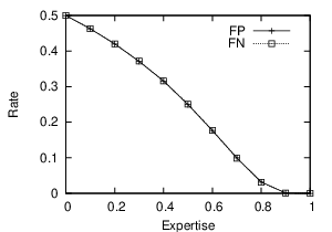
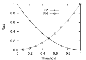
Figure 7 shows that both the FP and FN decrease when the expertise level of an IDS increases. We notice that the curves of FP rate and FN rate overlap. This is because the IDS detection density distributions are symmetric under $r=0$ and $r=1$. Figure 7 shows that the FP rate decreases with the decision threshold while the FN rate increases with the decision threshold. When the decision threshold is $0$, all feedback are positive (under-attack); when the decision threshold is $1$, all feedback are negative (no-attack).

One of the most important metrics to evaluate a feedback aggregation scheme is the cost of incorrect decisions. In this experiment, we study the costs of the three aggregation models using a simulated network. We set $N=10$ and fix the expertise level $l$ of all nodes to $0.5$ and set $C_{10}=C_{01}=1$ in (3) for the fairness of comparison, since the simple average and the weighted average models do not account for the cost difference between FP and FN. We fix the decision threshold for each IDS ($\tau_{p}$) to $0.1$ for the first batch run and then increase it by $0.1$ in each subsequent batch run until it reaches $0.9$. We measure the cost of the three models. As shown in Figure 7, the costs yielded by the aggregation using hypothesis testing remains the lowest among the three under all threshold settings. The costs of the weighted average and the simple average are close to each other. This is because in this experiment, the weights of all IDSs are the same. Therefore, the difference between the weighted average and the simple average is not substantial. We also observe that changing the threshold has a big impact on the costs of the weighted average and the simple average, while the cost of the hypothesis testing changes only slightly with the thresholds. All costs reach a minimum when the threshold is $0.5$ and increase when it deviates from $0.5$.

In the next experiment, the expertise levels of all nodes remain $0.5$ and their decision thresholds vary from $0.1$ to $0.9$. We set $C_{10}=C_{01}=1$ in the first batch run and increase $C_{01}$ by $1$ in every subsequent batch run. We observe the costs under three different models. Figure 7 shows that the costs of the simple average model and the weighted average model increase linearly with $C_{01}$ while cost of hypothesis testing model grows the slowest among the three. This is because the hypothesis testing model has a flexible threshold to optimize its cost. The hypothesis testing model has superiority when the cost difference between FP and FN is large.

In this experiment, we study the number of acquaintances needed for consultation to reach a predefined goal. Suppose the TP lower-bound $\bar{P}_{D}=0.95$ and FP upper-bound $\bar{P}_{F}=0.1$. We observe the change of FP rate and TP rate with the number of acquaintances consulted ($n$). Figure 7 shows that FP rate decreases and TP rate increases with $n$. Consulting higher expertise nodes leads to a higher TP rate and a lower FP rate. In the next experiment we implement Algorithm 1 on each node and measure the average number of acquaintances needed to reach the predefined TP lower-bound and the FP upper-bound. Figure 7 compares the simulation results with the theoretical results (see (22)), where the former confirms the latter. In both cases, the number of consultations decreases quickly with the expertise levels of acquaintances. For example, the IDS needs to consult around $50$ acquaintances of expertise $0.2$, while only $3$ acquaintances of expertise $0.7$ are needed for the same purpose. This is partly because low expertise nodes are more likely to make conflicting feedbacks and consequently increase the number of consultations. The analytical results can be useful for IDSs to design the size of their acquaintance lists.

References

- [1] P. Resnick, R. Zeckhauser, J. Swanson, and K. Lockwood, “The value of reputation on eBay: A controlled experiment,” Experimental Economics, vol. 9, no. 2, pp. 79–101, 2006.
- [2] C. Duma, M. Karresand, N. Shahmehri, and G. Caronni, “A trust-aware, p2p-based overlay for intrusion detection,” in DEXA Workshops, 2006.
- [3] C. Fung, J. Zhang, I. Aib, and R. Boutaba, “Robust and scalable trust management for collaborative intrusion detection,” in 11th IFIP/IEEE International Symposium on Integrated Network Management, 2009.
- [4] R. Janakiraman and M. Zhang, “Indra: a peer-to-peer approach to network intrusion detection and prevention,” Proceedings of the 12th IEEE International Workshops on Enabling Technologies, 2003.
- [5] V. Yegneswaran, P. Barford, and S. Jha, “Global intrusion detection in the domino overlay system,” in Proceedings of Network and Distributed System Security Symposium, 2004.
- [6] M. Cai, K. Hwang, Y. Kwok, S. Song, and Y. Chen, “Collaborative internet worm containment,” IEEE Security & Privacy, vol. 3, no. 3, pp. 25–33, 2005.
- [7] A. Ghosh and S. Sen, “Agent-based distributed intrusion alert system,” in Proceedings of the 6th International Workshop on Distributed Computing (IWDC’04). Springer, 2004.
- [8] C. Fung, O. Baysal, J. Zhang, I. Aib, and R. Boutaba, “Trust management for host-based collaborative intrusion detection,” in 19th IFIP/IEEE International Workshop on Distributed Systems, 2008.
- [9] J. Tsitsiklis, “Decentralized detection,” Advances in Statistical Signal Processing, pp. 297–344, 1993.
- [10] K. Nguyen, T. Alpcan, and T. Başar, “A Decentralized Bayesian Attack Detection Algorithm for Network Security,” in Proceedings of the 23rd International Information Security Conference, 2005.
- [11] A. Wald, Sequential Analysis. John Wiley and Sons, 1947.
- [12] B. C. Levy, Principles of Signal Detection and Parameter Estimation. Springer-Verlag, 2008.