Model Data Fusion: developing Bayesian inversion to constrain equilibrium and mode structure

With the advent of large scale neutral beam heating, magnetically confined fusion plasmas have drifted from the simple picture of ideal magnetohydrodynamics (MHD), which describes the plasma as a single, stationary, isotropic Maxwellian fluid. Due principally to neutral beam heating, several tokamak experiments now boast plasma toroidal rotation speeds that approach the thermal Mach speed and have significant stored energy residing in the energetic particle population produced by charge exchange with thermals. Motivated by these developments, a range of new descriptions have emerged that include thermal rotation [1] as well as energetic particles [2]. Despite this, ideal MHD is still the foundation of nearly all analysis. Detailed magnetic reconstruction based on this treatment ignores the energetic complexity of the plasma, and can result in model-data inconsistencies, such as thermal pressure profiles which are inconsistent with the total stored kinetic energy of the plasma.

A parallel development has been the improvement in the diversity, accuracy and resolution of plasma diagnostics. Interpretation, however, often requires a detailed knowledge of the plasma equilibrium. For example, inference of the toroidal current profile $j_{\phi}(\psi)$ from line of sight measurements of the polarization angle requires a knowledge of the poloidal flux $\psi$ across the plasma. Formally, diagnostic forward functions relate the vector of plasma parameters $\mathbf{\mathcal{I}}$ to the measurement vector $\mathbf{\mathcal{D}}$. For a linear system, such as toroidal current inference in a double null configuration, $\mathbf{\mathcal{I}}$ and $\mathbf{\mathcal{D}}$ are normally related through a response matrix $\mathbf{\mathcal{M}}$ with additional contributions $\mathbf{\mathcal{C}}$, such that $\mathbf{\mathcal{D}}=\mathbf{\mathcal{M}}\mathbf{\mathcal{I}}+\mathbf{\mathcal{C}}$. Inference involves inverting this relationship to give plasma parameters $\mathbf{\mathcal{I}}$ that are consistent with the data $\mathbf{\mathcal{D}}$. A widespread technique used is least-square fitting, in which prior assumptions are included via a penalty term in the fit.

The confluence of higher performance plasmas with diagnostic development has however led to a dichotomy: data is often inconsistent with ideal MHD equilibria, sometimes misleading scientists to propose new phenomena to describe data “artifacts”. An example is filamentation of flux surfaces in the Rijhnuizen Tokamak, which was inferred from fluctuations in measurements of electron temperature [3]. Subsequent analysis of the Thomson scattering detection chain revealed that with the correct photoelectron statistics and 2D instrument profile, similar structures could arise from noise. [4, 5].

Recently, a new integrated data-modelling approach for inference of fusion plasma parameters has emerged which offers a natural framework with which to resolve artifacts from model behaviour. In contrast to least square fitting, the Bayesian approach to inference involves the specification of an initial prior probability distribution function (pdf), $P(\mathbf{\mathcal{I}})$, which is then updated by taking into account information that the measurements provide through the likelihood pdf $P(\mathbf{\mathcal{D}}|\mathbf{\mathcal{I}})$. The result is the posterior distribution $P(\mathbf{\mathcal{I}}|\mathbf{\mathcal{D}})$ given by Bayes’ formula

$$P(\mathbf{\mathcal{I}}|\mathbf{\mathcal{D}})=P(\mathbf{\mathcal{D}}|\mathbf{\mathcal{I}})P(\mathbf{\mathcal{I}})/P(\mathbf{\mathcal{D}}).$$

(1)

The advantage of the Bayesian approach over traditional inversion techniques is two-fold: (i) prior knowledge, including known parameter inter-dependencies is made explicit, and (ii) as the formulation is probabilistic, random errors, systematic uncertainties and instrumental bias are integral part of the analysis rather than an afterthought.

In this work we present initial results of forward models of current tomography in the Mega Ampere Spherical Tokamak (MAST), we formulate Bayesian inference of force balance, and we identify plans for inference of mode structure in the H1 heliac. The paper is structured as follows: Sec. 2 briefly outlines the MAST experiment and present first results for Bayesian inference of poloidal flux and current profiles from MAST motional Stark effect (MSE) measurements. Section 3 outlines a Bayesian inference framework for force balance, synthesizes a pressure profile posterior given the flux surfaces from MSE and Thomson Scattering data, and computes an estimate of $f(\psi)f^{\prime}(\psi)$, with $f(\psi)$ the toroidal flux function. Using this, we are able to quantify the impact of poloidal currents on the equilibrium configuration. Section 4 outlines a Bayesian inference model for mode structure and develops a plasma model to compute candidate modes in the H-1 heliac. Finally, Sec. 5 contains concluding remarks.

The Mega Ampere Spherical Tokamak, which first published physics results in 2001 [6], is one of the world’s largest spherical tokamaks. While MAST physics and technology development have contributed across a broad range of fusion science [7, 8], two properties of MAST help motivate this research: high performance, and precision diagnostics. It is the combination of these properties in a spherical tokamak, which has a relatively weak toroidal field and therefore large sensitivity to poloidal currents compared to conventional tokamaks, which helps motivate selection of MAST to develop Bayesian inference for force balance.

Recently, both MAST neutral beam injectors have been upgraded to 3.8 MW. This has enabled plasma performance to be routinely lifted above $\beta_{n}\approx 5$, which was reported in 2005 [9]. MAST is equipped with an array of precision diagnostics [8], including a high spatial resolution, single-time point, ruby Thomson Scattering system, a multi-time point Nd:YAG Thomson Scattering system with a coarser spatial resolution, Motional Stark effect, Charge Exchange Recombination, and fast magnetics [10].

Our development of Bayesian inference of the current profile on MAST closely follows the seminal work of Svensson and Werner [11]. In that work, the plasma was represented as a grid of toroidal axisymmetric current beams, each with rectangular cross-section and each beam carrying a uniform current density. In MAST, we have placed these beams so as to fill-out the entire limiter region as depicted in Figure 1. The magnetic field generated is a summation of Biot-Savart’s law over current beams.

A key advantage to using a series of current beams with finite cross-section to model the plasma current (as opposed to a filamentary model) is that the semi-analytic expressions for the corresponding magnetic field and vector potential have no singularities, even at points within the current beam itself. Indeed, if one were to use filaments to model the plasma current, there would be many singular points in the calculated magnetic field within the plasma that would make subsequent flux-surface calculations difficult and somewhat questionable [11].

The physics goal of our work is to exploit the improved resolution of diagnostics to infer the validity of different force balance descriptions. Specifically, we have in mind development of a framework that will validate energetic plasma resolved force balance models. To build towards this goal, we commence by applying Bayesian inference to the axisymmetric Grad-Shafranov equilibrium description of ideal MHD force balance, $\mathbf{J}\times\mathbf{B}=\nabla P$.

The well known Grad-Shafranov equation [13] can be written

$$F(R,Z)=0$$

(16)

where

	$\displaystyle\hskip-28.45274ptF(R,Z)$	$\displaystyle\hskip-8.5359pt=$	$\displaystyle\hskip-8.5359pt-\mu_{0}Rj_{\phi}(\psi)+\mu_{0}R^{2}p^{\prime}(\psi)+\mu_{0}^{2}f(\psi)f^{\prime}(\psi),$		(17)
	$\displaystyle\hskip-28.45274pt-\mu_{0}Rj_{\phi}(\psi)$	$\displaystyle\hskip-8.5359pt=$	$\displaystyle\hskip-8.5359ptR\frac{\partial}{\partial R}\frac{1}{R}\frac{\partial\psi}{\partial R}+\frac{\partial^{2}\psi}{\partial z^{2}}.$		(18)

For a real plasma, the presence of nonideal effects will mean $F(R,Z)$ is nonzero. Our long term aim is to compute $P(\mathbf{\mathcal{F}}|\mathbf{\mathcal{D}})$ using Bayes formula, such that $P(\mathbf{\mathcal{D}}|\mathbf{\mathcal{F}})=P(\mathbf{\mathcal{D}}|\mathbf{\mathcal{F}})P(\mathbf{\mathcal{F}})/P(\mathbf{\mathcal{D}})$. Here,the vector $\mathbf{\mathcal{D}}$ comprises all the magnetics, motional Stark effect, Thomson scattering and charge exchange recombination data, while the column vector $\mathbf{\mathcal{F}}$ contains $F(R,Z)$ evaluated from Eq. (17) at different $(R,Z)$ across the plasma.

An integral representation for the prior $P(\mathbf{\mathcal{F}})$ can be obtained by using the transformation property

	$\displaystyle\hskip-28.45274ptP(\mathbf{\mathcal{F}},p^{\prime}(\psi),f(\psi)f^{\prime}(\psi)\times\left|{\frac{\partial(\mathbf{\mathcal{F}},p^{\prime}(\psi),f(\psi)f^{\prime}(\psi))}{\partial(j_{\phi}(\psi),p^{\prime}(\psi),f(\psi)f^{\prime}(\psi))}}\right|=$
	$\displaystyle P(j_{\phi}(\psi),p^{\prime}(\psi),f(\psi)f^{\prime}(\psi))$		(19)

and integrating both sides across $\mathbf{p}$ and $\mathbf{f}$. That is,

$$\hskip-28.45274ptP(\mathbf{\mathcal{F}})=\int\frac{P(j_{\phi}(\psi),p^{\prime}(\psi),f(\psi)f^{\prime}(\psi))}{\left|{\frac{\partial(\mathbf{\mathcal{F}},p^{\prime}(\psi),f(\psi)f^{\prime}(\psi))}{\partial(j_{\phi}(\psi),p^{\prime}(\psi),f(\psi)f^{\prime}(\psi))}}\right|}dp^{\prime}dff^{\prime}(\psi)$$

(20)

where the integrand $dp^{\prime}dff^{\prime}=dp^{\prime}(\psi)df(\psi)f^{\prime}(\psi)$. An ideal MHD plasma satisfies Eq. (16), such that the residual force is zero, and so $P(\mathbf{\mathcal{F}})=\delta(\mathbf{\mathcal{F}})$. Unfortunately, the joint distribution function $P(j_{\phi}(\psi),p^{\prime}(\psi),f(\psi)f^{\prime}(\psi))$ is non-separable, preventing direct integration of Eq. (20). In future work we will fold interdependency of $j_{\phi},p^{\prime}$ and $f(\psi)f^{\prime}(\psi)$ together to enable calculation of $P(j_{\phi}(\psi),p^{\prime}(\psi),f(\psi)f^{\prime}(\psi)$.

A second objective of the project is to test predictions of MHD mode theory, particularly mode structure. To achieve this goal we intend to develop a Bayesian inference tool to identify oscillations using the mode structure of a collection of candidate modes. The low beta heliac plasma configuration of H-1NF is ideally suited to this task, as there is little uncertainty in the equilibrium, and precision control of the helical coil currents enables access to a wide range of magnetic rotational transform ($\,\iota\!\!$-) profiles, as shown in Fig. 6. The combination thus offers a rich testing ground for Bayesian mode analysis.

For inference of mode structure, the relevant plasma parameters $\mathbf{\mathcal{I}}$ are the set of eigenmode-specifying parameters (frequency, mode numbers, radial structure moments) and $\mathbf{\mathcal{D}}$ is a set of Mirnov array measurements made outside the plasma. By solving the eigenmode problem in the plasma, and computing the vacuum-region magnetic field corresponding to a given plasma mode we obtain the forward model for $\mathbf{\mathcal{D}}$ given $\mathbf{\mathcal{I}}$. Given some prior $P(\mathbf{\mathcal{I}})$, the likelihood $P(\mathbf{\mathcal{D}}|\mathbf{\mathcal{I}})$ can then be constructed.

In the remainder of this section we derive the forward model for Global Alfvén Eigenmodes (GAEs) in H-1 plasmas. As a starting point to this sub-task, we compute GAEs in a cylindrical plasma model (coordinates $(r,\theta,z)$) incorporating a vacuum region in the region $r_{p}<r<r_{w}$ which is encased by a perfectly conducting wall at $r=r_{w}$.

GAEs are discrete modes that accumulate at the minimum $\omega_{min}^{2}$ of the Alfvén continuum $\omega_{A}^{2}=k_{\parallel}^{2}v_{A}^{2}$[15] where $k_{\parallel}$ denotes the component of the wave vector parallel to the equilibrium magnetic field and $v_{A}$ denotes the Alfvén speed. Expanding $k_{\parallel}=\mathbf{k}\cdot\mathbf{B}$ and substituting into $\omega_{A}^{2}=k_{\parallel}^{2}v_{A}^{2}$ yields $\omega_{A}^{2}\propto(n-\mbox{$\,\iota\!\!$-}m)^{2}/\rho$ where $m,n$ are the poloidal and toroidal mode numbers respectively, and $\rho$ is the mass density profile, assumed to take the form $\rho=\rho_{0}\left({1-r^{2}/r_{p}^{2}}\right)$ with $\rho_{0}$ the density on-axis. We define $\omega_{min}^{2}$ to be the global minimum of $\omega_{A}^{2}$ over the interval $(0,r_{p})$, if such a minimum exists. That is, $\omega_{min}^{2}$ is the smallest $\omega_{A}^{2}(r_{0})$ with both ${\omega_{A}^{2}}^{\prime}(r_{0})=0$ and ${\omega_{A}^{2}}^{\prime\prime}(r_{0})>0$ for some radius $r_{0}$ such that $0<r_{0}<r_{p}$. Figure 7 shows the dependency of $\omega_{min}$ on $\kappa_{h}$ for different $m$, $n$ modes. We have restricted our attention to the frequency interval $0<f<40$ kHz, where $f=\omega/(2\pi)$, since we are only interested in stable modes, and current H-1 diagnostics cannot resolve frequencies above 40 kHz. Theoretically, for a given $\kappa_{h}$, GAEs lie at frequencies just below the lines in Figure 7, accumulating at $\omega_{min}$, with an increasing number of radial nodes the closer the eigenfrequency lies to $\omega_{min}$.

We have modelled the plasma region by a stellarator normal-mode formulation in a cylindrical plasma [16, 17], corrected for non constant density profile. The eigenvalue equation for this problem can be written

$$L\varphi=\omega^{2}M\varphi,$$

(22)

where $\omega$ is given in units of inverse Alfvén time $\tau_{A}^{-1}=B_{0}/R\sqrt{\mu_{0}\rho_{0}}$, with $B_{0}$ the field strength at the magnetic axis, and where $\varphi$ is defined in terms of the radial element of the fluid displacement

$$r\xi_{r}=\exp{\left[{i(m\theta-\frac{n}{R}z)}\right]}\varphi(r),$$

(23)

with $i=\sqrt{-1}$. The operators $L$ and $M$ are give by:

	$\displaystyle\hskip-28.45274ptL$	$\displaystyle=$	$\displaystyle-\frac{1}{r}\frac{d}{dr}(n-m\mbox{$\,\iota\!\!$-})^{2}r\frac{d}{dr}+$		(24)
			$\displaystyle\frac{m^{2}}{r^{2}}\left[(n-m\mbox{$\,\iota\!\!$-})^{2}-D_{S}+\frac{\ddot{\mbox{$\,\iota\!\!$-}}}{m}(n-m\mbox{$\,\iota\!\!$-})\right],$
	$\displaystyle\hskip-28.45274ptM$	$\displaystyle=$	$\displaystyle-\frac{1}{r}\frac{d}{dr}\frac{\rho(r)}{\rho_{0}}r\frac{d}{dr}+\frac{\rho(r)}{\rho_{0}}\frac{m^{2}}{r^{2}}.$		(25)

Equation (22) is derived by averaging over helical ripple and assuming large aspect ratio. The Suydam stability parameter is given by

$$D_{S}=-\frac{\beta_{0}}{2\epsilon^{2}}p^{\prime}(r)\Omega^{\prime}(r)$$

(26)

where the average field line curvature is

$$\Omega(r)=\epsilon^{2}N\left(r^{2}\mbox{$\,\iota\!\!$-}+2\int{r\mbox{$\,\iota\!\!$-}}dr\right)$$

(27)

Here $j=\sqrt{-1}$, ’prime’ denotes radial derivatives, $\dot{\mbox{$\,\iota\!\!$-}}=r\mbox{$\,\iota\!\!$-}^{\prime}$, $p(r)$ is the normalized pressure, $\epsilon$ is the inverse aspect ratio, $N$ is the number of turns made by the helical windings and $\beta_{0}=2\mu_{0}p_{0}/B_{0}^{2}$ is the ratio of plasma pressure to magnetic pressure at magnetic axis.

Turning now to the vacuum region, the magnetic field $B$ must satisfy $\nabla\times B=0$ and $\nabla\cdot B=0$. In cylindrical geometry we can write $B$ in terms of modified Bessel functions, up to a scale factor.[18] The boundary conditions

$$[[B_{r}]]=[[B_{\parallel}]]=0$$

(28)

where $[[B]]=B_{vacuum}-B_{plasma}$, together with

	$\displaystyle\xi_{r}(0)$	$\displaystyle=$	$\displaystyle 0,|m|\neq 1,$		(29)
	$\displaystyle\xi_{r}^{\prime}(0)$	$\displaystyle=$	$\displaystyle 0,|m|=1,$		(30)
	$\displaystyle B_{r}(r_{w})$	$\displaystyle=$	$\displaystyle 0,$		(31)

relate the vacuum solution to that in the plasma.

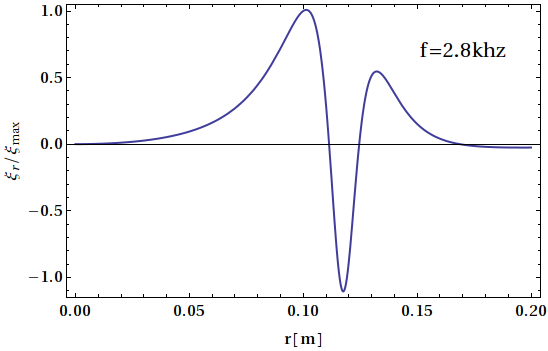
If $\omega_{min}^{2}$ appears in the plasma and is positive, a shooting method is used to find solutions to Eqs. (22), (28), (31), and Eq. (29) or Eq. (30) with frequency $0<\omega<\omega_{min}$. More explicitly, we select the appropriate boundary condition for $\xi_{r}$ at $r=0$, and then ’shoot’ out to the plasma/vacuum interface, searching frequency space in the region $0<\omega<\omega_{min}$ for eigenfrequencies that are consistent with Eq. (28). Figure 8 shows an example of an $(m,n)=(3,4)$ eigenmode found in this manner, located at the point $(\kappa_{h},\omega)$ indicated by the cross-hairs in Figure 7. The global structure seen has promising features when compared to recent spectral measurements of the mode: the mode structure is global in radial extent, and the radial position of the peaks nodes broadly matches observations.

In this work we have described a Bayesian inversion framework for inference of force-balance and mode structure. Progress has been reported in three areas: development of Bayesian inversion for current profiles; inference of the toroidal flux profile assuming the plasma satisfied ideal MHD; and calculation of a Global Alfvén eigenmnodes in a helical-ripple averaged cylindrical plasma model.

Based on working by Svensson et al. we have developed Bayesian inversion for current profiles and poloidal flux contours in MAST. The model comprises a grid of rectangular toroidally extended current beams, and is constrained by pickup coils, flux looops and MSE data. Owing to the placement of the MSE viewing optics the tangent of the polarisation angle of emitted light is linear in $B_{R}$ and $B_{Z}$. Signals from the pickup coils and flux loops are also linear in $B_{R}$ and $B_{Z}$. This feature means the prediction vector for the data is linear in the currents. We have used a conditional autoregresssive prior to describe the initial current distribution, which has the advantage of enforcing some smoothness between adjacent current beams while minimizing spatially long ranged effects. Posterior calculations of the poloidal flux contours of MAST #22254 at 320 ms illustrate good boundary agreement to EFIT.

In Sec. 3 we outlined an inference technique for the extraction of force balance, as applied to the Grad Shafranov equation. Using Thomson scattering data and a Monte Carlo simulation technique, we fitted pressure profiles to the inboard midplane chord of MAST, and computed $p^{\prime}(\psi)$. Assuming ideal MHD force balance we then calculated $f(\psi)f^{\prime}(\psi)$. While the $f(\psi)f^{\prime}(\psi)$ profile is similar to EFIT, the change in $f(\psi)$ from the core to the edge is 22%, which is slightly larger than the EFIT value. Qualitatively, this poloidal current should lift the on-axis safety factor by $\approx 22$%, and increase the change in poloidal flux across the plasma, but not change the geometry of flux surfaces or the Shafranov shift. At present, we are substituting the corrected $B_{\phi}$ profile inferred from $f(\psi)$ into MINERVA to compute the effect of poloidal currents on the calculation of $j_{\phi}$ and $\psi$ surfaces. This constitutes a first step towards combining $j_{\phi},p^{\prime}(\psi)$ and $f(\psi)f^{\prime}(\psi)$ to validate different equilibrium descriptions.

Finally, we have developed an analysis approach for the inference of mode structures, and constructed a GAE model. The model, which is in cylindrical geometry, accounts for a non constant density profile, features helical ripple averaging to compute the Suydam criterion and generate $\,\iota\!\!$-, and includes the vacuum region. The model has been applied to the range of $\,\iota\!\!$- profiles accessible to H-1 plasmas, and the minimum in the continuum computed as a function of helical winding current ratio $\kappa_{h}$. The eigenfunction of a candidate $(m,n)=(3,4)$ GAE mode was determined at an angular frequency of 12.1 krad s^-1. The eigenfunction has similar structure to recent observations in H1, including the same number of radial nodes which occur at similar radial positions.

In ongoing work we are developing forward models of Thomson scattering and charge exchange recombination spectroscopy for inference of force balance in MAST plasmas. We will be exploiting this information not only to improve equilibrium reconstruction, but to use Bayesian inference as a tool with which to resolve competing equilibrium models. In particular, we intend to compare force balance descriptions of ideal MHD, ideal MHD with flow [1], two fluid models [19], and energetic fluid resolved equilibria [2]. The Bayesian model offers a rigorous framework with which to quantify the fit and thereby elucidate the important underlying physics. With regards mode structure, we intend to transform the cylindrical eigenfunction to a beam cross-section equilibria [20] and identify a candidate mode set which spans the different type of mode structures observed. The next stage of this work involves deployment of forward models for mode structures into MINERVA to compute the posterior for the mode class and parameters. On a longer time scale we envisage the cylindrical plasma model will be replaced by a fully 3D ideal MHD wave mode code, CAS3D [21]. As with equilibrium modelling, the importance of mode analysis by Bayesian inversion is that it offers a rigorous framework in which to identify wave mode structures, some of which have deleterious effects on plasma performance.

References

- [1] L. Guazzotto, R. Betti, J. Manickam, and S. Kaye, Phys. Plasmas 11, 604 (2004).
- [2] M. J. Hole and G. Dennis, Plas. Phys. Con. Fus. 51, 035014 (2009).
- [3] N. J. L. Cardozo et al., Phys. Rev. Lett. 73, 256 (1994).
- [4] B. P. van Milligen, I. G. J. Classen, and C. J. Barth, Rev. Sci. Instrum. 74, 3998 (2003).
- [5] N. J. L. Cardozo et al., Phys. Rev. Lett. 90, 0031 (2003).
- [6] A. Sykes et al., Phys. Plas. 8, 2101 (2001).
- [7] B. Lloyd and et al, Nuc. Fus. 47, S658 (2007).
- [8] H. Meyer and et al, Nuc. Fus. 49, 104017 (2009).
- [9] M. Hole et al., Plas.Phys. Con. Fus. 47, 581 (2005).
- [10] M. J. Hole, L. C. Appel, and R. Martin, Rev. Sci. Instrum. (2009), submitted.
- [11] J. Svensson and A. Werner, Plas. Phys. Cont. Fus. 50, 085002 (2008).
- [12] J. Besag, Journal of the Royal Statistical Society. Series B 36, 192 (1974).
- [13] J. Wesson, Tokamaks, 2nd ed. (Oxford Univ. Press, Oxford, 1997).
- [14] W. H. Press, S. A. Teukolsky, W. T. Vetterling, and B. P. Flannery, Numerical Recipes in Fortran 77: The Art of Scientific Computing, 2nd ed. (Univ. of Cambridge Press, Cambridge, 1997).
- [15] K. Appert, R. Gruber, F. Troyon, and J. Vaclavik, Plas. Phys. 24, 1147 (1982).
- [16] T. Tatsuno and M. Wakatani, Nucl. Fusion 39, 1391 (1999).
- [17] R. L. Dewar et al., Phys. Rev. E 70, 0066409 (2004).
- [18] D. W. Ross, G. L. Chen, and S. M. Mahajan, Phys. Fluids 25, 652 (1982).
- [19] K. G. McClements and A. Thyagaraja, Mon. Not. R. Astron. Soc. 323, 733 (2001).
- [20] M. G. Davidson, R. L. Dewar, H. J. Gardner, and J. Howard, Aus. J. Phys. 48, 871 (1995).
- [21] C. Schwab, Phys. Fluids B - Plas. Phys. 9, 3195 (1993).