跳到论文正文
W Papers独立论文阅读器 arXiv:1002.3103 论文正文 计算阅读时间 · 0%
引用这篇论文根据当前论文元数据生成,正式投稿前建议核对。


License: CC BY-NC-SA 3.0
arXiv:1002.3103v1 [cond-mat.stat-mech] 16 Feb 2010

Infinite Cycles in Boson Lattice Models

Gerard Gordon Boland

a thesis submitted to
the national university of ireland
for the degree of

doctor of philosophy

by

Based on research carried out in the

School of Mathematical Sciences,

College of Engineering, Mathematical and Physical Sciences,

University College Dublin

under the direction of Professor Joseph V. Pulé
Head of School: Dr. Mícheal Ó Searcóid

University College Dublin \todaymonth

Abstract

We study the relationship between long cycles and Bose-Einstein condensation (BEC) in the case of several models. A convenient expression for the density of particles on cycles of length qq is obtained, in terms of qq unsymmetrised particles coupled with a boson field.

Using this formulation we reproduce known results on the Ideal Bose Gas, Mean-Field and Perturbed Mean-Field Models, where the condensate density exactly equals the long cycle density.

Then we consider the Infinite-Range-Hopping Bose-Hubbard Model:

HVBH=12​V​∑x,y=1V(ax∗−ay∗)​(ax−ay)+λ​∑x=1Vnx​(nx−1)H^{\rm BH}_{V}=\frac{1}{2V}\!\sum_{x,y=1}^{V}(a^{\ast}_{x}-a^{\ast}_{y})(a^{\phantom{*}}_{x}-a^{\phantom{*}}_{y})+\lambda\sum_{x=1}^{V}n_{x}(n_{x}-1)

in two cases, first for λ=+∞\lambda=+\infty, otherwise known as the hard-core boson model; and secondly for λ\lambda finite, representing a finite on-site repulsion interaction.

For the hard-core case, we find we may disregard the hopping contribution of the qq unsymmetrised particles, allowing us to calculate an exact expression for the density of particles on long cycles. It is shown that only the cycle of length one contributes to the cycle density. We conclude that while the existence of a non-zero long cycle density coincides with the occurrence of Bose-Einstein condensation, the respective densities are not necessarily equal.

For the case of a finite on-site repulsion, we obtain an expression for the cycle density involving the partition function for a Bose-Hubbard Hamiltonian with a single-site correction again by neglecting the qq unsymmetrised hop. Inspired by the Approximating Hamiltonian method we conjecture a simplified expression for the short cycle density as a ratio of single-site partition functions. In the absence of condensation we prove that this simplification is exact and use it to show that in this case the long-cycle density vanishes. In the presence of condensation we can justify this simplification when a gauge-symmetry breaking term is introduced in the Hamiltonian. Assuming our conjecture is correct, we compare numerically the long-cycle density with the condensate and again find that though they coexist, in general they are not equal.

Acknowledgements

I am extremely indebted to Professor Joseph V. Pulé for his guidance, encouragement and patience. He never failed to be a source of inspiration, happy to explain everything from the deepest methodologies to the slightest of mathematical details, and when leaving me with the impression he was several steps ahead, always waited patiently for me to catch up. My introduction to Quantum Statistical Mechanics has been thorough and exciting due to his tireless efforts, for which I am eternally grateful.

I thank the external examiner Professor Valentin Zagrebnov for a careful and thorough reading of the thesis and several helpful comments and suggestions for its improvement.

I also wish to thank Professor Teunis C. Dorlas for his many inputs in my education, always eager to suggest ideas, offer help and propose a new topic for discussion.

To all the friends I have made in the process of studying for this Ph.D., especially those of us who all began together; Alex Byrne, Ian Harris, Anna Heffernan, Liquin Tao, Barry Wardell, and in particular Thomas Jaeck, Ciara Morgan and Anne Ghesquiere, I want to say it is a pleasure to know you all. And thanks to those who have known me even longer, especially Cormac, Eleanor, John, Odhran, Terry and Harriet. I am lucky to have such good friends.

Also I wish to thank the administrative staff of UCD, who helped me navigate through the mire of paperwork with ease, and went out of their way to ensure everything ran smoothly.

I acknowledge the support of the Irish Research Council for Science, Engineering and Technology.

Finally I must thank my parents, my sisters Leonie and Maureen, my uncle Michael and my niece Kate, whom I always know I can depend on when I need some encouragement, distraction, comfort and humility.

Go raibh míle maith agaibh go leor.

Chapter 1 Introduction


Summary
To begin it is useful to look back through the literature to trace the progression of discoveries made by many great minds on the phenomenon of Bose-Einstein condensation in quantum statistical mechanics. We discuss the order parameters that have been postulated to indicate the presence of this condensate, and give details on all known about their relationships to date. Finally we briefly detail the layout of this thesis.


1.1 Bose-Einstein Condensation

In 1925, the phenomenon of Bose-Einstein condensation was predicted by Einstein following correspondence with S.N. Bose, who had found a novel derivation of photon statistics and the Planck distribution [36]. Einstein extended these ideas to an ideal monatomic gas [37] and observed that below some critical temperature, a number of molecules which grows with the total density, transition to an “unmoving state,” and this condensed substance coexists with the monatomic gas. These papers appeared about a year before the development of Quantum Mechanics and was the first time the wave nature of matter was explored, with particles obeying the same statistics as photons.

Since then we now know that all particles in nature can be classified into two classes according to their intrinsic angular momentum or spin. Those with half-integer spin are called fermions, those with integral spin are bosons. Fermions are restricted by the Pauli-Exclusion principle, which prevent multiple fermions from existing in the same quantum state, however bosons have no such restriction. The aforementioned “unmoving state” is now known to consist of bosons at (or near) the bosonic ground state, with particles in this state denoted as the (generalised) Bose-Einstein condensate (BEC).

Nevertheless at the time, Einstein’s claim of a phase transition in the ideal bose gas was dismissed, largely due to the criticism in 1927 of G. Uhlenbeck [83] (a graduate student of P. Ehrenfest) who argued that a gas of finitely many particles can exhibit no discontinuity, which was technically correct at the time, as it was yet to be shown that singularities in thermodynamic functions are a consequence of the thermodynamic limit (i.e. second-order phase transitions). This opinion prevailed until 1937 when H.A. Kramers pointed out the importance of the limit, causing Uhlenbeck [84] to withdraw his objections and assert that Einstein’s formula for the particle number-density is correct in the thermodynamic limit.

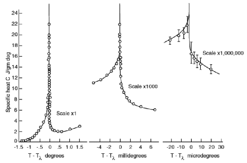
Meanwhile although the experimentalist H. Kamerlingh Onnes [85] had succeeded in liquifying Helium (4He) in 1908, it was not until 1928 that his student W.H. Keesom with M. Wolfke [55] discovered that at temperatures below 2.18K, a second phase of liquid helium appears, and christened it Helium II. Four years later Keesom and K. Clusius [54] measured the famous peak in the specific heat of helium, whose shape inspired the name λ\lambda-transition for the behaviour at the critical temperature Tλ=2.18​KT_{\lambda}=2.18K (see Figure 1.1). Further research [53, 3] in 1938 into Helium II found that a portion of the liquid flows without any apparent viscosity, a phenomenon now called superfluidity.
Refer to caption
Figure 1.1: The λ\lambda-transition in 4He.

In 1937 F. London [62] connected this curious phase transition in 4He (a bosonic gas) with the disputed ideas of Einstein on the ideal gas. He noted that Einstein’s formula for the transition temperature was a good estimate for TλT_{\lambda} and consequently introduced the concept of macroscopic occupation of the ground state and related it to the coherence properties of the condensate. That the superfluidity of 4He is due to the presence of Bose-Einstein condensation is now a fact which is largely accepted today.

Cowley and Woods [23] in 1968 were the first to experimentally detect condensate at T=1.1​KT=1.1K. Later work [2, 27] repeated and improved these experiments and found the critical temperature to be 2.24±0.04​K2.24\pm 0.04K, closely matching the corresponding value for the lambda-point TλT_{\lambda}, lending weight to a correspondence between condensation and superfluidity. A more thorough historical account of these discoveries can be found in [47]. While BEC has been proved experimentally, nevertheless it remains a valuable concept to the quantum statistical mechanics community as it is the only known phase-transition taking place in the absence of interactions, its origin being purely quantum mechanical.[4]

A general theory for condensation of interacting bosonic gasses remain to this day a notoriously difficult problem. The theory of the ideal gas has led to the formulation that “Bose-Einstein condensate” labels those particles which occupy lowest kinetic energy state, i.e.

ϱ0ρ=limV→∞⟨N0⟩V.\varrho^{\rho}_{0}=\lim_{V\to\infty}\frac{\langle N_{0}\rangle}{V}.

A rigourous proof that ϱ0ρ>0\varrho^{\rho}_{0}>0 for systems with realistic inter-particle interactions is an ongoing pursuit. In 1947 N.N. Bogoliubov computed the excitation spectrum for the weakly interacting Bose gas and pointed out the similarities with the spectrum of Helium II. This implied that the inclusion of interactions in the model had little effect upon the condensate, but instead had a pronounced impact upon the wave function.

Until recently in fact, BEC had not been proved for many-body Hamiltonians with genuine interactions except for one special case: hard core bosons on a lattice at half-filling, i.e., number of particles is exactly half the number of sites, in 1978 [35, 56]. Five years later in 1983, E. Buffet, Ph. de Smedt and J.V. Pulé [20] showed the existence of BEC for a class of homogeneous bosonic systems with interactions close to the van der Walls limit with a gap in the one-particle excitation spectrum. Independently in 2002, E. Lieb and R. Seiringer [60] considered a model of an interacting system of a trapped (and thus inhomogeneous) gas in the Gross-Pitaevski limit. J. Lauwers, A. Verbeure and V.A. Zagrebnov [58] in 2003, proved the occurrence of zero-mode Bose-Einstein condensation for a class of continuous homogeneous systems of boson particles with super-stable interactions and a one-particle energy gap.

Because of the difficulty of treating the boson gas interacting through a pair potential, various approximations have been proposed. One approach is to isolate the portion of the interaction which depends only upon the occupation numbers, separating the interaction it into a diagonal part (with respect to the occupation number basis) and an off-diagonal part (see [59]). K. Huang, C.N. Yang and J.M. Luttinger in 1957 [50] argued that some of the diagonal terms can enhance the amount of condensate, while Bogoliubov and his school claimed that it contains terms which deplete it. C.N Yang and C.P. Yang [98] considered a special case in d=1d=1 of a repulsive delta potential and prove that it exhibits no phase transition (see also [32, 31]). However considering the diagonal portion of this interaction alone, the Hamiltonian reduces to that of the Huang-Yang-Luttinger model which has a guaranteed phase transition at d=1d=1. This points to the idea that the off-diagonal terms must suppress this condensate, which indicates a more complex interplay of the diagonal and off-diagonal portions of the interaction than previously thought. Select models considering only the diagonal terms include the Mean-Field model [24, 91], the Huang-Yang-Luttinger model [89, 88], the Perturbed Mean-Field model [87, 28], and the Full-Diagonal model [29], all of which can possess a critical phase.

Another model which has been considered includes non-diagonal BCS-type interaction terms in addition to the diagonal terms [70, 100].

Analysis of further models was made possible by two Ansätze by Bogoliubov, the first to truncate the full Hamiltonian of the interacting bosons to produce the Weakly Imperfect Bose Gas (WIBG)[99], the second to perform apt substitutions of some operators by cc-numbers, known as the Bogoliubov approximation. Condensation is shown to appear in the WIBG (with some peculiarities). Investigations into the experimentally observed Mott insulator-superfluid (or condensate) phase transition [44] resulted in the analysis of the so-called Bose-Hubbard model, proposed by Fisher et. al. [43], and successfully analysed using the Bogoliubov approximation in [17, 30] to exhibit BEC.

1.2 The Feynman-Kac Integral and Cycle Lengths

An alternative parameterisation to predict the occurrence of the condensate was postulated by R.P. Feynman in 1953 [42]. He was discouraged by the fact that energies of a complex system are “hopelessly” difficult to calculate, so he tried combine his path integral formulation with Bose statistics to see if a transition could be found by other means.

The idea behind the Feynman path integral can be traced back to a paper by Dirac [26] in 1933 on an alternative formulation of quantum mechanics. Initially the quantum theories concurrently developed by Heisenberg and Schrödinger and others in the 1920 were built as a close analogy to classical mechanics where they considered the Hamiltonian HH, an energy function of coordinates and momenta. Dirac found that the Lagrangian LL, a function of the coordinates x⁡(t)x(t) and velocities x˙​(t)\dot{x}(t), to be more intuitive than the Hamiltonian approach. His reasoning is as follows, in classical dynamics the action is given by

S⁡[x⁡(⋅)]=∫L⁡(x˙​(t),x⁡(t))​𝑑tS[x(\,\cdot\,)]=\int L(\dot{x}(t),x(t))dt (1.1)

where the integral is taken between initial and final times 00 and tt. The action must depend on the path x⁡(⋅)x(\,\cdot\,) taken by the particles, and hence is a functional of these paths. The principle of least action states that for small variations of these paths, the action SS is minimised. He hoped that these classical paths could somehow be useful to describe the evolution of a quantum particle.

In his article, Dirac considers the time propagation operator e−itH/ℏ\mathrm{e}^{-itH/\hbar}. For two points xx and yy in a region Λ\Lambda, quantum mechanics tells us that we can write the probability Pt​(x,y)P_{t}(x,y) that a particle with initial position xx propagates to position yy after time tt, as Pt​(x,y)=|Kt​(x,y)|2P_{t}(x,y)=|K_{t}(x,y)|^{2}, the square of the amplitudes

K(x,y;t)=⟨y|e−itH/ℏ|x⟩.K(x,y;t)=\langle y|\mathrm{e}^{-itH/\hbar}|x\rangle.

This amplitude is the sum of the amplitudes of all possible paths which start at xx and end at yy after time tt. We will denote such a path by ωx,yt:[0,t]→Λ\omega^{t}_{x,y}:[0,t]\to\Lambda and denote its amplitude by K⁡[ωx,yt]K[\omega^{t}_{x,y}]. Let Ωx,yt\Omega^{t}_{x,y} be the set of all these paths. Then

K⁡(x,y,t)=∑ω∈Ωx,ytK⁡[ωx,yt].K(x,y;t)=\sum_{\omega\in\Omega^{t}_{x,y}}K[\omega^{t}_{x,y}].

We would like to see how each path ωx,yt\omega^{t}_{x,y} contributes to the total amplitude. Dirac suggests that the amplitude K⁡[ωx,yt]K[\omega^{t}_{x,y}] “corresponds to” the quantity

exp⁡{iℏ​S​[ωx,yt​(t)]}\exp\left\{\frac{i}{\hbar}S[\omega^{t}_{x,y}(t)]\right\}

and later writes that it is the “classical analogue” of the propagator.

By 1948 Feynman [41] had developed this suggestion and showed it was more than an analogy: it was an equality. He succeeded in formulating his “space-time approach,” deriving a third formulation of Quantum Mechanics using this expression for the propagator in terms of the action (a formulation later shown to be equivalent to the Heisenberg and Schrödinger pictures). And while Dirac considered only the classical path, Feynman showed that all paths contribute: in a sense, the quantum particle takes all paths, and the amplitudes for each path add according to the usual quantum mechanical rule for combining amplitudes. What was lacking was a rigourous definition of summing over these paths.

Surprisingly a well-defined calculus of such paths was already well known to mathematicians by the 1920s, due to N. Wiener and his study of stochastic processes and Brownian motion (extending the earlier work of Einstein and M. Smoluchowski). He introduced the concept of integration in functional spaces that now bears his name: the Wiener measure and Wiener integral. In 1949, Kac [51] considered Feynman’s path integral and realised that if one replaces the time parameter in the Dirac-Feynman expression for the action, equation (1.1), with a purely imaginary time, the Feynman path integral becomes a Wiener integral which (with some work) can be written in terms of the Hamiltonian H=H0+VH=H_{0}+V:

K(x,y;t→−iℏβ)=⟨y|e−β​H|x⟩=∫Wx​yβ(dω)exp{−∫0βV(ω(s))ds}K(x,y;t\to-i\hbar\beta)=\langle y|\mathrm{e}^{-\beta H}|x\rangle=\int W^{\beta}_{xy}(d\omega)\exp\left\{-\int_{0}^{\beta}V(\omega(s))ds\right\}

which is now called the Feynman-Kac path-integral.

Returning to Feynman’s proposition of an order parameter for BEC, he started out by analysing the partition function for a system of nn particles interacting via a pair potential of the form V⁡(x,y)=V⁡(|x−y|)V(x,y)=V(|x-y|). Using the Feynman-Kac formula, one can write the e−β​H\mathrm{e}^{-\beta H},

K(x1,…,xn;y1,…,yn)=∫Wβx1,y1(dω1)⋯∫Wβxn,yn(dωn)×exp{−∑j<k∫0βV(ωj(s)−ωk(s))ds}K(x_{1},\dots,x_{n};y_{1},\dots,y_{n})=\int W^{\beta}_{x_{1},y_{1}}(d\omega_{1})\cdots\int W^{\beta}_{x_{n},y_{n}}(d\omega_{n})\\ \times\exp\left\{-\sum_{j<k}\int_{0}^{\beta}V(\omega_{j}(s)-\omega_{k}(s))ds\right\} (1.2)

where the Wiener measure Wx,yβ​(ω)W^{\beta}_{x,y}(\omega) describes a Brownian path that starts at xx and ends at yy with “time” β\beta, i.e. ω⁡(0)=x\omega(0)=x and ω⁡(β)=y\omega(\beta)=y.

The Feynman path integral has become a very powerful tool in Statistical Mechanics. For a system of bosons with Hamiltonian HH, the canonical partition function can be written as

ZV​(n)=trace​[σ+​e−β​H]=1n!​∑π∈Sn∫d​x1​…​d​xn​K​(x1,…,xn,xπ⁡(1),…,xπ⁡(n))Z_{\hbox{\tiny{$V$}}}(n)=\text{\rm{trace}}\,\left[\sigma_{+}\mathrm{e}^{-\beta H}\right]=\frac{1}{n!}\sum_{\pi\in S_{n}}\int dx_{1}\dots dx_{n}K(x_{1},\dots,x_{n};x_{\pi(1)},\dots,x_{\pi(n)}) (1.3)

where the sum over permutations appears because we take the trace over the symmetric states (as indicated by σ+\sigma_{+}), and we integrate over all particle positions. (See Appendix A of [81] for a clear derivation of this expression).

Refer to caption
Figure 1.2: An interpretation of the Feynman-Kac representation of the partition function for a gas of bosons. The horizontal plane represents the dd spatial dimensions, and the vertical axis is the imaginary time direction. This picture considers five particles on two cycles, one of length 1 and the other of length 4 (Picture from [81]).

In Statistical Mechanics, β\beta is the inverse temperature. However if one were consider it as a time parameter for the Feynman-Kac formula, then one returns to the intuitive picture of moving particles following paths. Then equation (1.2) can be thought of as nn particles with initial positions xix_{i} and final positions yiy_{i} at “time” β\beta.

Now if one considers the integrand of the partition function expression (1.3), one sees that the initial and final positions for the particles are fixed, but a particle with initial position xix_{i} will have final position xπ⁡(i)x_{\pi(i)}, thus its path will depend upon the permutation π\pi.

Figure 1.2 provides an example, where five particles propagate in the imaginary time direction on paths with endpoints specified by the permutation

π=(1234524135)=(1243)​(5).\pi=\left(\begin{array}[]{ccccc}1&2&3&4&5\\ 2&4&1&3&5\end{array}\right)=(1243)(5).

The particle labelled five is on a closed Brownian bridge, starting and ending at the point x5x_{5}. We shall say this is a cycle of length one, whereby it took one timestep β\beta for the particle to return to its original position.

However the particle labelled one however lands on a different site, x2x_{2}, after time β\beta. Should it continue its journey, it will land at x4x_{4} at time 2​β2\beta, x3x_{3} at time 3​β3\beta and back to its starting position x1x_{1} after four timesteps. We shall call this a cycle of length four.

Feynman considered the probability that a given particle belongs to a cycle of length, say qq, and questioned if there was a strictly positive probability that, after taking the thermodynamic limit, a cycle of infinite length exist? He postulated that the occurrence of infinite (long) cycles is indicative of the presence of BEC.

Three years after Feynman’s conjecture, O. Penrose and L. Onsager [67] introduced a different order parameter for BEC, related to the concept of “off-diagonal long-range order” (OLDRO) [97] which investigates the correlation between two particles at positions xx and yy, i.e.

Dρ​(x,y)=limn/V=ρn,V→∞⟨ax∗​ay⟩.D_{\rho}(x,y)=\lim_{\stackrel{{\scriptstyle n,{\hbox{\tiny{$V$}}}\to\infty}}{{n/{\hbox{\tiny{$V$}}}=\rho}}}\langle a^{\ast}_{x}a^{\phantom{*}}_{y}\rangle.

We say the system displays OLDRO when Dρ​(x,y)>0D_{\rho}(x,y)>0 when |x−y|→∞|x-y|\to\infty. This correlation can be expressed in the Feynman-Kac representation, which involves an open cycle starting at xx and finishing at yy which may wind many times around the imaginary time direction (see Figure 1.3):

Dρ(x,y)=limn/V=ρn,V→∞1ZV​(n)​V1(n−1)!∫dx2…dxn∑π∈Sn∫dWβx1,x^π⁡(1)(ω1)⋯∫dWβxn,x^π⁡(n)(ωn)×exp{−∑j<k∫0βV(ωj(s)−ωk(s))ds}D_{\rho}(x,y)=\lim_{\stackrel{{\scriptstyle n,{\hbox{\tiny{$V$}}}\to\infty}}{{n/{\hbox{\tiny{$V$}}}=\rho}}}\frac{1}{Z_{\hbox{\tiny{$V$}}}(n)V}\frac{1}{(n-1)!}\int dx_{2}\dots dx_{n}\sum_{\pi\in S_{n}}\int dW^{\beta}_{x_{1},\hat{x}_{\pi(1)}}(\omega_{1})\cdots\int dW^{\beta}_{x_{n},\hat{x}_{\pi(n)}}(\omega_{n})\\ \times\exp\left\{-\sum_{j<k}\int_{0}^{\beta}V(\omega_{j}(s)-\omega_{k}(s))ds\right\} (1.4)

where we have set x1=x,x^1=yx_{1}=x,\hat{x}_{1}=y and x^j=xj\hat{x}_{j}=x_{j} for j=2,…,nj=2,\dots,n. As |x−y|→∞|x-y|\to\infty there corresponds a notion of infinite winding which is reminiscent of Feynman’s approach. Penrose and Onsager observed that there should be BEC when the fraction of the total particle number belonging to infinite cycles is strictly positive.

Refer to caption
Figure 1.3: Interpretation of Off-Diagonal Long-Range Order in terms of Feynman-Kac integrals

It was generally agreed at the time that this parameter is the correct one for BEC, however infinite cycles were still considered noteworthy, with for instance a possible role in superfluidity [68], and showing analogous phase transitions to various physical processes such as percolation, gelation and polymerisation, see for example [22, 75, 76, 25].

However it was not until 1993 that A. Sütő [78, 79] gave a precise mathematical and quantitative formulation relating the occurrence of BEC (and hence OLDRO) with the existence of infinite cycles. He proved in the cases of the free bose gas and the mean field gas that in fact infinite cycles do occur below the transition temperature for BEC. In 2001, D. Ueltschi [82] considered a simple lattice model in which the integral over Brownian paths is replaced by an effective weight. He proved that infinite cycles do not occur for high temperatures. Later in 2003, T.C. Dorlas, Ph. Martin and J.V. Pulé [34] considered a model of a Bose gas with some genuine short range interactions between modes using the theory of Large Deviations developed by Varadhan [95], and proved that the average fraction of infinite cycles is equal to the density of condensate.

However more recent investigations cast doubt upon the suitability of infinite cycles as an order parameter for BEC. Ueltschi [82] argues that both order parameters are identical in the case of a weakly interacting Bose gas, but in the presence of a strong inter-particle interaction this correlation breaks down. The example offered is a crystalline system. The off-diagonal correlation function decays exponentially as the inter-particle distance increases so there in no OLDRO. However Brownian motion occurs as a consequence of the interchange of particles via quantum tunnelling. Due to the strong interaction, these Brownian paths need to avoid each other, which for dimensions greater than two and for low enough temperatures can result in a macroscopic number of particles on random walks of infinite length.

As a result there exists uncertainty as to exactly what connection there is between Bose-Einstein condensation and infinite cycles, which motivates the subject of this thesis. Here we compare the long cycle density with that of the condensate for two models of interacting bosons, both of which involve an on-site repulsive interaction.

We find a weaker result than [34], that the existence of long cycles coincides with the presence of BEC, but their respective densities are not necessarily equal. In fact, the long cycle density can be both greater than or less than the condensate density. It appears that the single-site repulsion term can either increase or decrease the quantity of long cycles, depending upon the thermodynamic parameters of the system. Nevertheless this analysis does lend weight to Feynman’s conjecture in the absence of strong interactions.

Outline of Thesis

The object of this thesis is to study the relation between the occurrence of BEC and the existence of infinite cycles for some Boson lattice models, in particular the infinite-range-hopping Bose-Hubbbard model with both hard cores and without. These models correspond to bosonic systems that describe particles hopping on a lattice and interacting among themselves with the constraint that their wavefunctions are invariant under permutations of the particles. The partition function can induce a probability measure upon the set of permutations, with which one can calculate expectations of cycle lengths.

In Chapter 2 we apply the techniques for cycle statistics described in [34], following [64], to establish the general framework for evaluating the density of particles on cycles of particular lengths, and show that this formulation uniquely partitions the particles into their cycle structures.

In Chapter 3 we formulate a relation between occupation numbers and the cycle structure of models which satisfy particular conditions, which implies the condensate density equals the infinite cycle density. We then check the conditions in the case of three simple models, the Ideal Bose Gas, the Mean-Field Bose Gas and the Perturbed Mean-Field Bose gas, to reproduce the results of Sütő [78, 79] and Dorlas, Martin and Pulé [34].

In Chapter 4 we consider the Infinite-Range-Hopping Bose-Hubbard Model with hard-cores, i.e. infinite on-site repulsion to prevent multiple particles occupying individual sites. We calculate the density of particles on cycles on infinite length and compare the result with the condensate density.

In Chapter 5 we consider the Infinite-Range-Hopping Bose-Hubbard Model (without hard-cores) where now there is a finite on-site repulsion to discourage multiple particles per site. Again we consider infinite cycle density and compare the result with the condensate density.

Chapter 2 Cycle Statistics


Summary
In this chapter we will introduce a general framework for cycle statistics by expanding the bosonic partition function into a sum over permutations of an unsymmetrised trace term and inducing a probability measure upon these permutations. By decomposing these permutations into their cycle structures, we derive a convenient expression for the density of particles on cycles of particular lengths, and show that this formulation uniquely partitions the particles depending upon the cycle lengths they live on. In taking the thermodynamic limit we define the long cycles to be those which are of infinite length, and short cycles as those which are finite in length. We find that we can uniquely decompose the total density of particles into those on long cycles and those on short cycles, i.e. ρ=ϱshort+ϱlong\rho=\varrho_{\rm short}+\varrho_{\rm long}. Finally we also obtain an expression for the expectation of certain operators in terms of cycle statistics, which will be useful for analysing occupation number densities and off-diagonal long-range order in later chapters.


2.1 Cycle Representation of the Partition Function

In his paper investigating the low-temperature properties of liquid He4, R. Feynman [42] re-expressed the partition function of a boson gas in terms of the cycle structures of permutations induced by Bose-Statistics. He postulated that at low temperatures (or high densities), bosons belong to cycles of different lengths, and below some critical temperature cycles of infinite length appear. Feynman associated this critical behaviour with the phase transition of He4 known as Bose-Einstein condensation.

In this chapter we will establish a general framework for cycle statistics as described in [34], following [64]. This framework will be applied throughout this script so it is valuable to lay down the notational foundation for this thesis before applying the techniques to various models.

To begin, we shall consider a system of nn identical bosons enclosed in a region Λ\Lambda with volume |Λ||\Lambda|, in thermal equilibrium at temperature TT (i.e. in the canonical ensemble). Denote the inverse temperature β:=kB​T\beta\vcentcolon=k_{B}T, where kBk_{B} is Boltzmann’s constant. For this ensemble we take the thermodynamic limit at a fixed temperature β\beta by letting the quantities nn and |Λ||\Lambda| tend to infinity in such a way that n/|Λ|=ρn/|\Lambda|=\rho for a fixed ρ\rho. For the entirety of this text we shall fix β\beta, and drop it from our notation where possible.

Denote the single particle Hilbert space by ℋΛ\mathcal{H}_{\hbox{\tiny{$\Lambda$}}}. Let II be the identity operator on ℋΛ\mathcal{H}_{\hbox{\tiny{$\Lambda$}}}. For an operator AA on ℋΛ\mathcal{H}_{\hbox{\tiny{$\Lambda$}}} denote A(n)A^{(n)} as the operator on an unsymmetrised (i.e. no Bose-statistics) nn-particle Hilbert space ℋΛ(n):=ℋΛ⊗ℋΛ⊗⋯⊗ℋΛ⏟n times{\mathcal{H}_{{\hbox{\tiny{$\Lambda$}}}}^{(n)}}\vcentcolon=\underbrace{\mathcal{H}_{\hbox{\tiny{$\Lambda$}}}\otimes\mathcal{H}_{\hbox{\tiny{$\Lambda$}}}\otimes\cdots\otimes\mathcal{H}_{\hbox{\tiny{$\Lambda$}}}}_{\text{$n$ times}} by

A(n)=A⊗I⊗⋯⊗I+I⊗A⊗⋯⊗I+⋯+I⊗⋯⊗I⊗A.A^{(n)}=A\otimes I\otimes\dots\otimes I+I\otimes A\otimes\dots\otimes I+\dots+I\otimes\dots\otimes I\otimes A.

When considering bosons, we need to restrict the system to the symmetric subspace of ℋΛ(n){\mathcal{H}_{{\hbox{\tiny{$\Lambda$}}}}^{(n)}}. Let SnS_{n} be the set of all permutations of {1,…,n}\{1,\dots,n\}. The symmetrisation projection σ+(n)\sigma_{+}^{(n)}\, on ℋΛ(n){\mathcal{H}_{{\hbox{\tiny{$\Lambda$}}}}^{(n)}} is defined by

σ+(n):=1n!​∑π∈SnUπ\sigma_{+}^{(n)}\,\vcentcolon=\frac{1}{n!}\sum_{\pi\in S_{n}}U_{\pi}

where Uπ:ℋΛ(n)↦ℋΛ(n)U_{\pi}:{\mathcal{H}_{{\hbox{\tiny{$\Lambda$}}}}^{(n)}}\mapsto{\mathcal{H}_{{\hbox{\tiny{$\Lambda$}}}}^{(n)}} is a unitary representation of the permutation group SnS_{n} on ℋΛ(n){\mathcal{H}_{{\hbox{\tiny{$\Lambda$}}}}^{(n)}} defined by

Uπ(ϕ1⊗ϕ2⊗⋯⊗ϕn)=ϕπ⁡(1)⊗ϕπ⁡(2)⊗⋯⊗ϕπ⁡(n)U_{\pi}(\phi_{1}\otimes\phi_{2}\otimes\cdots\otimes\phi_{n})=\phi_{\pi(1)}\otimes\phi_{\pi(2)}\otimes\cdots\otimes\phi_{\pi(n)}

with ϕj∈ℋΛ\phi_{j}\in\mathcal{H}_{\hbox{\tiny{$\Lambda$}}}, j=1,…,nj=1,\dots,n and any π∈Sn\pi\in S_{n}. Thus we denote the symmetric or bosonic nn-particle Hilbert space by ℋΛ,+(n):=σ+(n)​ℋΛ(n){\mathcal{H}_{{\hbox{\tiny{$\Lambda$}}},+}^{(n)}}\vcentcolon=\sigma_{+}^{(n)}\,{\mathcal{H}_{{\hbox{\tiny{$\Lambda$}}}}^{(n)}}. We assume that there is a symmetric Hamiltonian HΛnH_{\hbox{\tiny{$\Lambda$}}}^{n\phantom{j}} on ℋΛ(n){\mathcal{H}_{{\hbox{\tiny{$\Lambda$}}}}^{(n)}} whose restriction to ℋΛ,+(n){\mathcal{H}_{{\hbox{\tiny{$\Lambda$}}},+}^{(n)}} is the Boson Hamiltonian for our system. The canonical partition function for the nn-particle Hamiltonian HΛnH_{\hbox{\tiny{$\Lambda$}}}^{n\phantom{j}} can be written as

ZΛ​(n)=traceℋΛ,+(n)​[e−β​HΛn]=traceℋΛ(n)​[σ+(n)​e−β​HΛn]=1n!​∑π∈SntraceℋΛ(n)​[Uπ​e−β​HΛn].Z_{\hbox{\tiny{$\Lambda$}}}(n)=\text{\rm{trace}}\,_{{\mathcal{H}_{{\hbox{\tiny{$\Lambda$}}},+}^{(n)}}}\left[\mathrm{e}^{-\beta H_{\hbox{\tiny{$\Lambda$}}}^{n\phantom{j}}}\right]=\text{\rm{trace}}\,_{{\mathcal{H}_{{\hbox{\tiny{$\Lambda$}}}}^{(n)}}}\left[\sigma_{+}^{(n)}\,\mathrm{e}^{-\beta H_{\hbox{\tiny{$\Lambda$}}}^{n\phantom{j}}}\right]=\frac{1}{n!}\sum_{\pi\in S_{n}}\text{\rm{trace}}\,_{{\mathcal{H}_{{\hbox{\tiny{$\Lambda$}}}}^{(n)}}}\left[U_{\pi}\mathrm{e}^{-\beta H_{\hbox{\tiny{$\Lambda$}}}^{n\phantom{j}}}\right].

This leads us naturally to define a probability measure on SnS_{n} by

ℙΛn​(π)=1ZΛ​(n)​1n!​traceℋΛ(n)​[Uπ​e−β​HΛn]\mathbb{P}^{n}_{\hbox{\tiny{$\Lambda$}}}(\pi)=\frac{1}{Z_{\hbox{\tiny{$\Lambda$}}}(n)}\frac{1}{n!}\text{\rm{trace}}\,_{{\mathcal{H}_{{\hbox{\tiny{$\Lambda$}}}}^{(n)}}}\left[U_{\pi}\mathrm{e}^{-\beta H_{\hbox{\tiny{$\Lambda$}}}^{n\phantom{j}}}\right] (2.1)

provided that the following holds for all π∈Sn\pi\in S_{n}:

traceℋΛ(n)​[Uπ​e−β​HΛn]≥0.\text{\rm{trace}}\,_{{\mathcal{H}_{{\hbox{\tiny{$\Lambda$}}}}^{(n)}}}\left[U_{\pi}\mathrm{e}^{-\beta H_{\hbox{\tiny{$\Lambda$}}}^{n\phantom{j}}}\right]\geq 0. (2.2)

Note that in general this condition is not obviously satisfied. However if e−β​HΛn\mathrm{e}^{-\beta H_{\hbox{\tiny{$\Lambda$}}}^{n\phantom{j}}} has a Feynman-Kac representation, then (2.2) must be true.

In the grand-canonical ensemble, the number of particles is not fixed, so we must be prepared to deal with an arbitrary number of particles. To do so we construct the Fock space ℱ⁡(ℋΛ)\mathcal{F}(\mathcal{H}_{\hbox{\tiny{$\Lambda$}}}) which consists of the tensor product of each canonical nn-particle Hilbert space ℋΛ(n){\mathcal{H}_{{\hbox{\tiny{$\Lambda$}}}}^{(n)}} for every n≥0n\geq 0. Then the thermodynamic limit simply consists of letting the region Λ\Lambda tend to ℝd\mathbb{R}^{d}. So

ℱ⁡(ℋΛ)=⨁n≥0ℋΛ(n)\mathcal{F}(\mathcal{H}_{\hbox{\tiny{$\Lambda$}}})=\bigoplus_{n\geq 0}{\mathcal{H}_{{\hbox{\tiny{$\Lambda$}}}}^{(n)}}

where ℋΛ(0):=ℂ{\mathcal{H}_{{\hbox{\tiny{$\Lambda$}}}}^{(0)}}\vcentcolon=\mathbb{C} and ℋΛ(1):=ℋΛ{\mathcal{H}_{{\hbox{\tiny{$\Lambda$}}}}^{(1)}}\vcentcolon=\mathcal{H}_{\hbox{\tiny{$\Lambda$}}}. Define the second quantization of the single-particle operator AA, denoted by d​Γ​(A)d\Gamma(A), as the operator which acts upon ℱ⁡(ℋΛ)\mathcal{F}(\mathcal{H}_{\hbox{\tiny{$\Lambda$}}}) by

d​Γ​(A)=⨁n≥0A(n)¯d\Gamma(A)=\overline{\bigoplus_{n\geq 0}A^{(n)}}

where A(0)=0A^{(0)}=0 and A(1)=AA^{(1)}=A. The number of particles is represented by the operator NΛ:=d​Γ​(I)N_{\hbox{\tiny{$\Lambda$}}}\vcentcolon=d\Gamma(I).

Again for the case of bosons, we need to restrict the system to the symmetric subspace of ℱ⁡(ℋΛ)\mathcal{F}(\mathcal{H}_{\hbox{\tiny{$\Lambda$}}}), denoted ℱ+​(ℋΛ)\mathcal{F}_{+}(\mathcal{H}_{\hbox{\tiny{$\Lambda$}}}), constructed by applying the symmetrisation operator to each ℋΛ(n){\mathcal{H}_{{\hbox{\tiny{$\Lambda$}}}}^{(n)}} in the tensor product:

ℱ+​(ℋΛ):=⨁n≥0ℋΛ,+(n)=⨁n≥0σ+(n)​ℋΛ(n)=⨁n≥01n!​∑π∈SnUπ​ℋΛ(n).\mathcal{F}_{+}(\mathcal{H}_{\hbox{\tiny{$\Lambda$}}})\vcentcolon=\bigoplus_{n\geq 0}{\mathcal{H}_{{\hbox{\tiny{$\Lambda$}}},+}^{(n)}}=\bigoplus_{n\geq 0}\sigma_{+}^{(n)}\,{\mathcal{H}_{{\hbox{\tiny{$\Lambda$}}}}^{(n)}}=\bigoplus_{n\geq 0}\frac{1}{n!}\sum_{\pi\in S_{n}}U_{\pi}{\mathcal{H}_{{\hbox{\tiny{$\Lambda$}}}}^{(n)}}.

The grand-canonical partition function for a system with Hamiltonian HΛH_{\hbox{\tiny{$\Lambda$}}} defined on the symmetric Fock space ℱ+​(ℋΛ)\mathcal{F}_{+}(\mathcal{H}_{\hbox{\tiny{$\Lambda$}}}) and with chemical potential μ\mu can be written as

ΞΛ​(μ)=traceℱ+​(ℋΛ)​[e−β⁡(HΛ−μ​NΛ)]=∑n=0∞1n!​∑π∈SntraceℋΛ(n)​[Uπ​e−β⁡(HΛ−μ​n)].\Xi_{\hbox{\tiny{$\Lambda$}}}(\mu)=\text{\rm{trace}}\,_{\mathcal{F}_{+}(\mathcal{H}_{\hbox{\tiny{$\Lambda$}}})}\left[\mathrm{e}^{-\beta(H_{\hbox{\tiny{$\Lambda$}}}-\mu N_{\hbox{\tiny{$\Lambda$}}})}\right]=\sum_{n=0}^{\infty}\frac{1}{n!}\sum_{\pi\in S_{n}}\text{\rm{trace}}\,_{{\mathcal{H}_{{\hbox{\tiny{$\Lambda$}}}}^{(n)}}}\left[U_{\pi}\mathrm{e}^{-\beta(H_{\hbox{\tiny{$\Lambda$}}}-\mu n)}\right].

We define the corresponding probability measure on ⋃n=0∞Sn\bigcup_{n=0}^{\infty}S_{n} by

ℙΛμ​(π)=1ΞΛ​(μ)​∑n=0∞1n!​traceℋΛ(n)​[Uπ​e−β⁡(HΛ−μ​n)]​ℐSn​(π)\mathbb{P}^{\mu}_{\phantom{l}\!\!{\hbox{\tiny{$\Lambda$}}}}(\pi)=\frac{1}{\Xi_{\hbox{\tiny{$\Lambda$}}}(\mu)}\sum_{n=0}^{\infty}\frac{1}{n!}\text{\rm{trace}}\,_{{\mathcal{H}_{{\hbox{\tiny{$\Lambda$}}}}^{(n)}}}\left[U_{\pi}\mathrm{e}^{-\beta(H_{\hbox{\tiny{$\Lambda$}}}-\mu n)}\right]\mathcal{I}_{S_{n}}(\pi)

(true if (2.2) is satisfied) where ℐ\mathcal{I} is the indicator function. We take S0={1}S_{0}=\{1\}.

Each permutation π∈Sn\pi\in S_{n} can be decomposed into a number of cyclic permutations of lengths q1,q2,…,qrq_{1},q_{2},\dots,q_{r} with r<nr<n and q1+q2+⋯+qr=nq_{1}+q_{2}+\dots+q_{r}=n. We consider the set Ω=⋃r∈ℕΩr\Omega=\bigcup_{r\in\mathbb{N}}\Omega_{r} of unordered rr-tuples of natural numbers 𝐪=[q1,q2,…,qr]∈Ωr\mathbf{q}=[q_{1},q_{2},\dots,q_{r}]\in\Omega_{r} for r=0,1,2,…r=0,1,2,\dots, and let |𝐪|=q1+q2+⋯+qr|\mathbf{q}|=q_{1}+q_{2}+\dots+q_{r} for 𝐪∈Ω\mathbf{q}\in\Omega. Then a decomposition of π∈Sn\pi\in S_{n} into cycles is labelled by 𝐪∈Ω\mathbf{q}\in\Omega with |𝐪|=n|\mathbf{q}|=n. We recall the following facts on the permutation group.

  • •

    The decomposition into cycles leads to a partition of SnS_{n} into equivalence classes of permutations C𝐪C_{\mathbf{q}}, |𝐪|=n|\mathbf{q}|=n.

  • •

    Two permutation π′\pi^{\prime} and π′′\pi^{\prime\prime} belong to the same class if and only if they are conjugate in SnS_{n}, i.e. if there exists a π∈Sn\pi\in S_{n} such that

    π′′=π−1​π′​π.\pi^{\prime\prime}=\pi^{-1}\pi^{\prime}\pi. (2.3)
  • •

    The number of permutations belonging to the class C𝐪C_{\mathbf{q}} is

    n!n𝐪!​(q1​q2​…​qr)\frac{n!}{n_{\mathbf{q}}!(q_{1}q_{2}\dots q_{r})} (2.4)

    with n𝐪!=n1!​n2!​…​nj!​…n_{\mathbf{q}}!=n_{1}!n_{2}!\dots n_{j}!\dots and njn_{j} is the number of cycles of length jj in 𝐪\mathbf{q}.

We observe for a symmetric Hamiltonian (i.e. [HΛ,Uπ]=0,∀π∈Sn[H_{\hbox{\tiny{$\Lambda$}}},U_{\pi}]=0,\forall\,\pi\in S_{n}), for π′,π′′∈C𝐪\pi^{\prime},\pi^{\prime\prime}\in C_{\mathbf{q}}, and using (2.3) one has that

traceℋΛ(n)​[Uπ′′​e−β​HΛn]=traceℋΛ(n)​[Uπ−1​Uπ′​Uπ​e−β​HΛn]=traceℋΛ(n)​[Uπ−1​Uπ′​e−β​HΛn​Uπ]=traceℋΛ(n)​[Uπ′​e−β​HΛn].\begin{split}\text{\rm{trace}}\,_{{\mathcal{H}_{{\hbox{\tiny{$\Lambda$}}}}^{(n)}}}\left[U_{\pi^{\prime\prime}}\mathrm{e}^{-\beta H_{\hbox{\tiny{$\Lambda$}}}^{n\phantom{j}}}\right]&=\text{\rm{trace}}\,_{{\mathcal{H}_{{\hbox{\tiny{$\Lambda$}}}}^{(n)}}}\left[U_{\pi}^{-1}U_{\pi^{\prime}}U_{\pi}\mathrm{e}^{-\beta H_{\hbox{\tiny{$\Lambda$}}}^{n\phantom{j}}}\right]\\ &=\text{\rm{trace}}\,_{{\mathcal{H}_{{\hbox{\tiny{$\Lambda$}}}}^{(n)}}}\left[U_{\pi}^{-1}U_{\pi^{\prime}}\mathrm{e}^{-\beta H_{\hbox{\tiny{$\Lambda$}}}^{n\phantom{j}}}U_{\pi}\right]\\ &=\text{\rm{trace}}\,_{{\mathcal{H}_{{\hbox{\tiny{$\Lambda$}}}}^{(n)}}}\left[U_{\pi^{\prime}}\mathrm{e}^{-\beta H_{\hbox{\tiny{$\Lambda$}}}^{n\phantom{j}}}\right].\end{split} (2.5)

Hence in the case of a symmetric Hamiltonian we may express the symmetrisation operator σ+(n)\sigma_{+}^{(n)}\, as a sum (with some scaling) over all unitary representations of permutations with unique cycle structures of SnS_{n} i.e.

traceℋΛ,+(n)​[e−β​HΛn]\displaystyle\text{\rm{trace}}\,_{{\mathcal{H}_{{\hbox{\tiny{$\Lambda$}}},+}^{(n)}}}\left[\mathrm{e}^{-\beta H_{\hbox{\tiny{$\Lambda$}}}^{n\phantom{j}}}\right] =∑C𝐪∑π∈C𝐪traceℋΛ(n)​[Uπ​e−β​HΛn]\displaystyle=\sum_{C_{\mathbf{q}}}\sum_{\pi\in C_{\mathbf{q}}}\text{\rm{trace}}\,_{{\mathcal{H}_{{\hbox{\tiny{$\Lambda$}}}}^{(n)}}}\left[U_{\pi}\mathrm{e}^{-\beta H_{\hbox{\tiny{$\Lambda$}}}^{n\phantom{j}}}\right]
=∑C𝐪n!n𝐪!​(q1​q2​…​qr)​traceℋΛ(n)​[Uπ​e−β​HΛn].\displaystyle=\sum_{C_{\mathbf{q}}}\frac{n!}{n_{\mathbf{q}}!(q_{1}q_{2}\dots q_{r})}\text{\rm{trace}}\,_{{\mathcal{H}_{{\hbox{\tiny{$\Lambda$}}}}^{(n)}}}\left[U_{\pi}\mathrm{e}^{-\beta H_{\hbox{\tiny{$\Lambda$}}}^{n\phantom{j}}}\right].

This motivates a more careful analysis of the class of cycle structures, specifically the expectation of cycles of particular lengths in C𝐪C_{\mathbf{q}}.

2.2 Cycle Densities

For q∈ℕq\in\mathbb{N}, define the random variable Nq​(π)N_{q}(\pi) to be the number of cycles of length qq in π\pi.

ℙΛn[Nq(π)=r]=∑Nq​(π)=rℙΛn(π).\mathbb{P}^{n}_{\hbox{\tiny{$\Lambda$}}}[N_{q}(\pi)\!=\!r]\,=\!\sum_{N_{q}(\pi)=r}\mathbb{P}^{n}_{\hbox{\tiny{$\Lambda$}}}(\pi).

Then we can define the expectation of cycles of length qq in the canonical ensemble by

𝔼Λn(Nq)=∑r=1nrℙΛn(Nq=r)=∑r=1n∑π∈SnrℙΛn[Nq(π)=r]\mathbb{E}^{n}_{\hbox{\tiny{$\Lambda$}}}(N_{q})=\sum_{r=1}^{n}r\mathbb{P}^{n}_{\hbox{\tiny{$\Lambda$}}}(N_{q}\!=\!r)=\sum_{r=1}^{n}\sum_{\pi\in S_{n}}r\mathbb{P}^{n}_{\hbox{\tiny{$\Lambda$}}}[N_{q}(\pi)\!=\!r]

and hence the average density of particles on qq-cycles for a system of nn bosons is

cΛn​(q)=q​𝔼Λn​(Nq)|Λ|.c_{\hbox{\tiny{$\Lambda$}}}^{n}(q)=\frac{q\;\mathbb{E}^{n}_{\hbox{\tiny{$\Lambda$}}}(N_{q})}{|\Lambda|}. (2.6)

We note here that if n/|Λ|=ρn/|\Lambda|=\rho then the sum of the densities of particles on all cycle lengths is exactly the density of the system, i.e.

∑q=1ncΛn​(q)=ρ.\sum_{q=1}^{n}c_{\hbox{\tiny{$\Lambda$}}}^{n}(q)=\rho. (2.7)

In the grand-canonical ensemble, we similarly obtain that the expectation of cycles of length qq is

𝔼Λμ​(Nq)=∑r=1∞r​ℙΛμ​(Nq=r),\mathbb{E}^{\mu}_{\hbox{\tiny{$\Lambda$}}}(N_{q})=\sum_{r=1}^{\infty}r\mathbb{P}^{\mu}_{\phantom{l}\!\!{\hbox{\tiny{$\Lambda$}}}}(N_{q}\!=\!r),

and so the average density of particles on qq-cycles is

cΛμ​(q)=q​𝔼Λμ​(Nq)|Λ|.c_{\hbox{\tiny{$\Lambda$}}}^{\mu}(q)=\frac{q\;\mathbb{E}^{\mu}_{\hbox{\tiny{$\Lambda$}}}(N_{q})}{|\Lambda|}. (2.8)

Define the grand-canonical expectation of the operator d​Γ​(A)d\Gamma(A) as

⟨d​Γ​(A)⟩HΛ=1ΞΛ​(μ)​traceℱ+​(ℋΛ)​[d​Γ​(A)​e−β⁡(HΛ−μ​NΛ)]=1ΞΛ​(μ)​∑n=0∞eβ​μ​n​ZΛ​(n)​⟨A(n)⟩HΛn.\langle d\Gamma(A)\rangle_{H_{\hbox{\tiny{$\Lambda$}}}}=\frac{1}{\Xi_{\hbox{\tiny{$\Lambda$}}}(\mu)}\text{\rm{trace}}\,_{\mathcal{F}_{+}(\mathcal{H}_{\hbox{\tiny{$\Lambda$}}})}\big[d\Gamma(A)\mathrm{e}^{-\beta(H_{\hbox{\tiny{$\Lambda$}}}-\mu N_{\hbox{\tiny{$\Lambda$}}})}\big]=\frac{1}{\Xi_{\hbox{\tiny{$\Lambda$}}}(\mu)}\sum_{n=0}^{\infty}\mathrm{e}^{\beta\mu n}Z_{\hbox{\tiny{$\Lambda$}}}(n)\langle A^{(n)}\rangle_{H_{\hbox{\tiny{$\Lambda$}}}^{n\phantom{j}}}. (2.9)

where

⟨A(n)⟩HΛn=1ZΛ​(n)​traceℋΛ,+(n)​[A(n)​e−β​HΛn].\langle A^{(n)}\rangle_{H_{\hbox{\tiny{$\Lambda$}}}^{n\phantom{j}}}=\frac{1}{Z_{\hbox{\tiny{$\Lambda$}}}(n)}\text{\rm{trace}}\,_{{\mathcal{H}_{{\hbox{\tiny{$\Lambda$}}},+}^{(n)}}}\left[A^{(n)}\mathrm{e}^{-\beta H_{\hbox{\tiny{$\Lambda$}}}^{n\phantom{j}}}\right]. (2.10)

The density of particles for finite volume is the expected number of particles per unit volume

ρΛ​(μ)=⟨NΛ⟩HΛ|Λ|.\rho_{\hbox{\tiny{$\Lambda$}}}(\mu)=\frac{\langle N_{\hbox{\tiny{$\Lambda$}}}\rangle_{H_{\hbox{\tiny{$\Lambda$}}}}}{|\Lambda|}.

Then the density of the system is the sum of all the cycle densities:

∑q=1∞cΛμ​(q)=ρΛ​(μ).\sum_{q=1}^{\infty}c_{\hbox{\tiny{$\Lambda$}}}^{\mu}(q)=\rho_{\hbox{\tiny{$\Lambda$}}}(\mu). (2.11)

Hence with this formulation, equations (2.7) and (2.11) imply that we can uniquely partition the ensemble of the particles into their respective cycle structures.

However we would like to observe the behaviour of these cycles in the thermodynamic limit. To do so we shall decompose the total system density into the density of particles belonging to cycles of finite length (ϱshort\varrho_{{\rm short}}) and to infinitely long cycles (ϱlong\varrho_{{\rm long}}) in the thermodynamic limit. We are thus led to the following definition:

Definition 1

The expected density of particles on cycles of infinite length is given

  • •

    in the canonical ensemble by

    ϱlongρ=limQ→∞limn/|Λ|=ρn,|Λ|→∞∑q=Q+1∞cΛn​(q),{\varrho^{\rho}_{{\rm long}}}=\lim_{Q\to\infty}\;\lim_{\stackrel{{\scriptstyle n,|\Lambda|\to\infty}}{{n/|\Lambda|=\rho}}}\;\sum_{q=Q+1}^{\infty}c_{\hbox{\tiny{$\Lambda$}}}^{n}(q),
  • •

    in the grand-canonical ensemble by

    ϱlongμ=limQ→∞lim|Λ|→∞∑q=Q+1∞cΛμ​(q).{\varrho^{\mu}_{{\rm long}}}=\lim_{Q\to\infty}\;\lim_{|\Lambda|\to\infty}\;\sum_{q=Q+1}^{\infty}c_{\hbox{\tiny{$\Lambda$}}}^{\mu}(q).

For notational convenience, we shall henceforth define limΛ\lim_{\Lambda} as the limit as Λ↑ℝd\Lambda\uparrow\mathbb{R}^{d}, where dd is the dimension of the system. The limited density in the grand-canonical ensemble is defined by ρ⁡(μ):=limΛρΛ​(μ){\rho(\mu)}\vcentcolon=\lim_{\Lambda}\rho_{\hbox{\tiny{$\Lambda$}}}(\mu).

Note that if we define the corresponding densities of short cycles as

ϱshortρ=limQ→∞limn/|Λ|=ρn,|Λ|→∞∑q=1QcΛn​(q),ϱshortμ=limQ→∞limΛ∑q=1QcΛμ​(q),{\varrho^{\rho}_{{\rm short}}}=\lim_{Q\to\infty}\;\lim_{\stackrel{{\scriptstyle n,|\Lambda|\to\infty}}{{n/|\Lambda|=\rho}}}\;\sum_{q=1}^{Q}c_{\hbox{\tiny{$\Lambda$}}}^{n}(q),\qquad\qquad{\varrho^{\mu}_{{\rm short}}}=\lim_{Q\to\infty}\;\lim_{\Lambda}\;\sum_{q=1}^{Q}c_{\hbox{\tiny{$\Lambda$}}}^{\mu}(q),

then using (2.7) and (2.11) one easily sees that

ρ=ϱshortρ+ϱlongρandρ⁡(μ)=ϱshortμ+ϱlongμ.\rho={\varrho^{\rho}_{{\rm short}}}+{\varrho^{\rho}_{{\rm long}}}\qquad\quad\text{and}\qquad\quad{\rho(\mu)}={\varrho^{\mu}_{{\rm short}}}+{\varrho^{\mu}_{{\rm long}}}.

Hence in the limit, all particles can be classified as those belonging to cycles of finite length and those belonging to cycles of infinite length.

2.3 Expression for the qq-cycle Density

Here we shall obtain a convenient expression for the density of particles on cycles of specific length in the following theorem. The idea is that since the trace of the partition function only depends upon the cycle structure of the symmetrisation operator, we can decompose this operator into its cycle distribution, isolate one qq cycle and then recombine the remaining cycles into a symmetrisation operator over n−qn-q particles leaving us with a trace over qq distinguishable particles coupled with a boson field (with some normalisation).

Before stating the theorem we first shall fix some notation. To indicate that a permutation π\pi contains at least one cycle of length qq, we shall say q∈πq\in\pi.

Let Uq:ℋΛ(q)→ℋΛ(q)U_{q}:{\mathcal{H}_{{\hbox{\tiny{$\Lambda$}}}}^{(q)}}\to{\mathcal{H}_{{\hbox{\tiny{$\Lambda$}}}}^{(q)}} be the unitary representation of a qq-cycle on ℋΛ(q){\mathcal{H}_{{\hbox{\tiny{$\Lambda$}}}}^{(q)}} defined by

Uq​(ϕ1⊗ϕ2⊗ϕ3⊗⋯⊗ϕq)=ϕ2⊗ϕ3⊗⋯⊗ϕq⊗ϕ1.U_{q}(\phi_{1}\otimes\phi_{2}\otimes\phi_{3}\otimes\dots\otimes\phi_{q})=\phi_{2}\otimes\phi_{3}\otimes\dots\otimes\phi_{q}\otimes\phi_{1}.

Denote the nn-space identity operator by In=I⊗I⊗⋯⊗I⏟n timesI_{n}=\underbrace{I\otimes I\otimes\cdots\otimes I}_{\text{$n$ times}} and the corresponding Fock space identity operator by 𝕀\mathbb{I}. When there is no ambiguity we shall simply write UqU_{q} for Uq⊗𝕀:ℱ+​(ℋV)→ℱ+​(ℋV)U_{q}\otimes\mathbb{I}:\mathcal{F}_{+}(\mathcal{H}_{\hbox{\tiny{$V$}}})\to\mathcal{F}_{+}(\mathcal{H}_{\hbox{\tiny{$V$}}}). Note that [Uq,σ+n]=0[U_{q},\sigma^{n}_{+}]=0.

Also we shall define the operator Mq,ΛμM^{\mu}_{q,{\hbox{\tiny{$\Lambda$}}}} on ℋΛ(q){\mathcal{H}_{{\hbox{\tiny{$\Lambda$}}}}^{(q)}} as the partial trace of e−β⁡(HΛ−μ​NΛ)\mathrm{e}^{-\beta(H_{\hbox{\tiny{$\Lambda$}}}-\mu N_{\hbox{\tiny{$\Lambda$}}})} over ℱ+​(ℋΛ)\mathcal{F}_{+}(\mathcal{H}_{\hbox{\tiny{$\Lambda$}}}), i.e.

Mq,Λμ=traceℱ+​(ℋΛ)​[e−β⁡(HΛ−μ​NΛ)].M^{\mu}_{q,{\hbox{\tiny{$\Lambda$}}}}=\text{\rm{trace}}\,_{\mathcal{F}_{+}(\mathcal{H}_{\hbox{\tiny{$\Lambda$}}})}\left[\mathrm{e}^{-\beta(H_{\hbox{\tiny{$\Lambda$}}}-\mu N_{\hbox{\tiny{$\Lambda$}}})}\right]. (2.12)
Theorem 2.1

The expectation of the density of particles on cycles of length qq can be expressed

  1. 1.

    in the canonical case as

    cΛn​(q)=1ZΛ​(n)​|Λ|​traceℋΛ(q)⊗ℋΛ,+(n−q)​[(Uq⊗In−q)​e−β​HΛn],c_{\hbox{\tiny{$\Lambda$}}}^{n}(q)=\frac{1}{Z_{\hbox{\tiny{$\Lambda$}}}(n)|\Lambda|}\;\text{\rm{trace}}\,_{{\mathcal{H}_{{\hbox{\tiny{$\Lambda$}}}}^{(q)}}\otimes{\mathcal{H}_{{\hbox{\tiny{$\Lambda$}}},+}^{(n-q)}}}\left[(U_{q}\otimes I_{n-q})\mathrm{e}^{-\beta H_{\hbox{\tiny{$\Lambda$}}}^{n\phantom{j}}}\right], (2.13)
  2. 2.

    in the grandcanonical ensemble as

    cΛμ​(q)=1ΞΛ​(μ)​|Λ|​traceℋΛ(q)⊗ℱ+​(ℋΛ)​[(Uq⊗𝕀)​e−β⁡(HΛ−μ​NΛ)]=1ΞΛ​(μ)​|Λ|​traceℋΛ(q)​[Uq​Mq,Λμ].\begin{split}c_{\hbox{\tiny{$\Lambda$}}}^{\mu}(q)&=\frac{1}{\Xi_{\hbox{\tiny{$\Lambda$}}}(\mu)|\Lambda|}\;\text{\rm{trace}}\,_{{\mathcal{H}_{{\hbox{\tiny{$\Lambda$}}}}^{(q)}}\otimes\mathcal{F}_{+}(\mathcal{H}_{\hbox{\tiny{$\Lambda$}}})}\left[(U_{q}\otimes\mathbb{I})\mathrm{e}^{-\beta(H_{\hbox{\tiny{$\Lambda$}}}-\mu N_{\hbox{\tiny{$\Lambda$}}})}\right]\\ &=\frac{1}{\Xi_{\hbox{\tiny{$\Lambda$}}}(\mu)|\Lambda|}\;\text{\rm{trace}}\,_{{\mathcal{H}_{{\hbox{\tiny{$\Lambda$}}}}^{(q)}}}\Big[U_{q}\,M^{\mu}_{q,{\hbox{\tiny{$\Lambda$}}}}\Big].\end{split} (2.14)
Proof 2.3.2.

Define Cn​(q1,n1,q2,n2,…,qr,nr)C_{n}(q_{1},n_{1};\,q_{2},n_{2};\dots;q_{r},n_{r}), qiq_{i} distinct, q1​n1+q2​n2+⋯+qr​nr=nq_{1}n_{1}+q_{2}n_{2}+\dots+q_{r}n_{r}=n as the class of permutations with the following cycle structure: n1n_{1} cycles of length q1q_{1}, n2n_{2} cycles of length q2q_{2}, etc. By (2.4) the number of elements in each class is

#​Cn​(q1,n1,q2,n2,…,qr,nr)=n!q1n1​…​qrnr​n1!​n2!​…​nr!.\#C_{n}(q_{1},n_{1};\,q_{2},n_{2};\dots;q_{r},n_{r})=\frac{n!}{q_{1}^{n_{1}}\dots q_{r}^{n_{r}}\,n_{1}!n_{2}!\dots n_{r}!}.

From (2.1)

ℙΛn​(Nq=r)=1ZΛ​(n)​1n!​∑(q1,…​qk≥0;qi≠q∑qi​ni=n−r​q)∑π∈Cn​(q,r,q1,n1,…,qk,nk)traceℋΛ(n)​[Uπ​e−β​HΛn].\mathbb{P}^{n}_{\hbox{\tiny{$\Lambda$}}}(N_{q}\!=\!r)=\frac{1}{Z_{\hbox{\tiny{$\Lambda$}}}(n)}\frac{1}{n!}\sum_{\begin{subarray}{c}{q_{1},\dots q_{k}\geq 0;\,q_{i}\neq q}\choose{\sum q_{i}n_{i}=n-rq}\end{subarray}}\sum_{\pi\in C_{n}(q,r;\,q_{1},n_{1};\dots;q_{k},n_{k})}\!\!\!\!\text{\rm{trace}}\,_{{\mathcal{H}_{{\hbox{\tiny{$\Lambda$}}}}^{(n)}}}\left[U_{\pi}\mathrm{e}^{-\beta H_{\hbox{\tiny{$\Lambda$}}}^{n\phantom{j}}}\right].

Using (2.5) we see that

ℙΛn​(Nq=r)=1ZΛ​(n)​1n!​∑(q1,…​qk≥0;qi≠q∑qi​ni=n−r​q)#​Cn​(q,r,q1,n1,…,qk,nk)×traceℋΛ(n)​[Uπ~​e−β​HΛn]\qquad\mathbb{P}^{n}_{\hbox{\tiny{$\Lambda$}}}(N_{q}\!=\!r)=\frac{1}{Z_{\hbox{\tiny{$\Lambda$}}}(n)}\frac{1}{n!}\sum_{\begin{subarray}{c}{q_{1},\dots q_{k}\geq 0;\,q_{i}\neq q}\choose{\sum q_{i}n_{i}=n-rq}\end{subarray}}\#C_{n}(q,r;\,q_{1},n_{1};\dots;q_{k},n_{k})\\ \times\text{\rm{trace}}\,_{{\mathcal{H}_{{\hbox{\tiny{$\Lambda$}}}}^{(n)}}}\left[U_{\tilde{\pi}}\mathrm{e}^{-\beta H_{\hbox{\tiny{$\Lambda$}}}^{n\phantom{j}}}\right]\qquad

where π~\tilde{\pi} is any fixed element in Cn​(q,r,q1,n1,…,qk,nk)C_{n}(q,r;\,q_{1},n_{1};\dots;q_{k},n_{k}). Therefore

ℙΛn​(Nq=r)=1ZΛ​(n)​1n!​∑(q1,…​qk≥0;qi≠q∑qi​ni=n−r​q)#​Cn​(q,r,q1,n1,…,qk,nk)#​Cn−q​(q,r−1,q1,n1,…,qk,nk)×#​Cn−q​(q,r−1,q1,n1,…,qk,nk)​traceℋΛ(n)​[Uπ~​e−β​HΛn]=1ZΛ​(n)​1n!​∑(q1,…​qk≥0;qi≠q∑qi​ni=n−r​q)n!r​q​(n−q)!×#​Cn−q​(q,r−1,q1,n1,…,qk,nk)​traceℋΛ(n)​[Uπ~​e−β​HΛn].\begin{split}\mathbb{P}^{n}_{\hbox{\tiny{$\Lambda$}}}(N_{q}\!=\!r)&=\frac{1}{Z_{\hbox{\tiny{$\Lambda$}}}(n)}\frac{1}{n!}\sum_{\begin{subarray}{c}{q_{1},\dots q_{k}\geq 0;\,q_{i}\neq q}\choose{\sum q_{i}n_{i}=n-rq}\end{subarray}}\tfrac{\#C_{n}(q,r;\,q_{1},n_{1};\dots;q_{k},n_{k})}{\#C_{n-q}(q,r-1;\,q_{1},n_{1};\dots;q_{k},n_{k})}\\ &\hskip 40.0pt\times\#C_{n-q}(q,r-1;\,q_{1},n_{1};\dots;q_{k},n_{k})\;\text{\rm{trace}}\,_{{\mathcal{H}_{{\hbox{\tiny{$\Lambda$}}}}^{(n)}}}\left[U_{\tilde{\pi}}\mathrm{e}^{-\beta H_{\hbox{\tiny{$\Lambda$}}}^{n\phantom{j}}}\right]\\[11.38092pt] &=\frac{1}{Z_{\hbox{\tiny{$\Lambda$}}}(n)}\frac{1}{n!}\sum_{\begin{subarray}{c}{q_{1},\dots q_{k}\geq 0;\,q_{i}\neq q}\choose{\sum q_{i}n_{i}=n-rq}\end{subarray}}\frac{n!}{rq(n-q)!}\\ &\hskip 40.0pt\times\#C_{n-q}(q,r-1;\,q_{1},n_{1};\dots;q_{k},n_{k})\;\text{\rm{trace}}\,_{{\mathcal{H}_{{\hbox{\tiny{$\Lambda$}}}}^{(n)}}}\left[U_{\tilde{\pi}}\mathrm{e}^{-\beta H_{\hbox{\tiny{$\Lambda$}}}^{n\phantom{j}}}\right].\end{split}

We choose one qq-cycle from π~\tilde{\pi}, since π~∈Cn​(q,r,q1,n1,…,qk,nk)\tilde{\pi}\in C_{n}(q,r;\,q_{1},n_{1};\dots;q_{k},n_{k}). Thus write π~=q∘π′\tilde{\pi}=q\circ\pi^{\prime}, where π′∈Cn−q​(q,r−1,q1,n1,…,qk,nk)\pi^{\prime}\in C_{n-q}(q,r-1;\,q_{1},n_{1};\dots;q_{k},n_{k}) and q∈π~q\in\tilde{\pi}. The corresponding representations can be written as Uπ~=Uq⊗Uπ′U_{\tilde{\pi}}=U_{q}\otimes U_{\pi^{\prime}}, so summing over π′\pi^{\prime}

ℙnΛ(Nq=r)=1ZΛ​(n)1r​q​(n−q)!∑(q1,…​qk≥0;qi≠q∑qi​ni=n−r​q)×∑π′∈Cn−q​(q,r−1,q1,n1,…,qk,nk)traceℋΛ(n)​[(Uq⊗Uπ′)​e−β​HΛn]\qquad\mathbb{P}^{n}_{\hbox{\tiny{$\Lambda$}}}(N_{q}\!=\!r)=\frac{1}{Z_{\hbox{\tiny{$\Lambda$}}}(n)}\frac{1}{rq(n-q)!}\sum_{\begin{subarray}{c}{q_{1},\dots q_{k}\geq 0;\,q_{i}\neq q}\choose{\sum q_{i}n_{i}=n-rq}\end{subarray}}\\ \times\hskip-6.0pt\sum_{\pi^{\prime}\in C_{n-q}(q,r-1;\,q_{1},n_{1};\dots;q_{k},n_{k})}\hskip-16.0pt\text{\rm{trace}}\,_{{\mathcal{H}_{{\hbox{\tiny{$\Lambda$}}}}^{(n)}}}\left[(U_{q}\otimes U_{\pi^{\prime}})\mathrm{e}^{-\beta H_{\hbox{\tiny{$\Lambda$}}}^{n\phantom{j}}}\right]\qquad

and by using (2.5) again we have

ℙnΛ(Nq=r)=1ZΛ​(n)1r​q​(n−q)!∑(q1,…​qk≥0;qi≠q∑qi​ni=n−r​q)×∑π′∈Cn−q​(q,r−1,q1,n1,…,qk,nk)traceℋΛ(n)​[(Uq⊗Uπ′)​e−β​HΛn].\qquad\mathbb{P}^{n}_{\hbox{\tiny{$\Lambda$}}}(N_{q}\!=\!r)=\frac{1}{Z_{\hbox{\tiny{$\Lambda$}}}(n)}\frac{1}{rq(n-q)!}\sum_{\begin{subarray}{c}{q_{1},\dots q_{k}\geq 0;\,q_{i}\neq q}\choose{\sum q_{i}n_{i}=n-rq}\end{subarray}}\\ \times\hskip-6.0pt\sum_{\pi^{\prime}\in C_{n-q}(q,r-1;\,q_{1},n_{1};\dots;q_{k},n_{k})}\hskip-16.0pt\text{\rm{trace}}\,_{{\mathcal{H}_{{\hbox{\tiny{$\Lambda$}}}}^{(n)}}}\left[(U_{q}\otimes U_{\pi^{\prime}})\mathrm{e}^{-\beta H_{\hbox{\tiny{$\Lambda$}}}^{n\phantom{j}}}\right].\qquad

Then the canonical expectation of the number of qq-cycles is found to be

𝔼Λn​(Nq)\displaystyle\mathbb{E}^{n}_{\hbox{\tiny{$\Lambda$}}}(N_{q}) =∑r=1∞r​ℙΛn​(Nq=r)\displaystyle=\sum_{r=1}^{\infty}r\mathbb{P}^{n}_{\hbox{\tiny{$\Lambda$}}}(N_{q}\!=\!r)
=1ZΛ​(n)1q⁡(n−q)!∑r=1∞∑(q1,…​qk≥0;qi≠q∑qi​ni=n−r​q)\displaystyle=\frac{1}{Z_{\hbox{\tiny{$\Lambda$}}}(n)}\frac{1}{q(n-q)!}\sum_{r=1}^{\infty}\sum_{\begin{subarray}{c}{q_{1},\dots q_{k}\geq 0;\,q_{i}\neq q}\choose{\sum q_{i}n_{i}=n-rq}\end{subarray}}
×∑π′∈Cn−q​(q,r−1,q1,n1,…,qk,nk)traceℋΛ(n)​[(Uq⊗Uπ′)​e−β​HΛn]\displaystyle\hskip 99.58464pt\times\hskip-6.0pt\sum_{\pi^{\prime}\in C_{n-q}(q,r-1;\,q_{1},n_{1};\dots;q_{k},n_{k})}\!\!\!\text{\rm{trace}}\,_{{\mathcal{H}_{{\hbox{\tiny{$\Lambda$}}}}^{(n)}}}\left[(U_{q}\otimes U_{\pi^{\prime}})\mathrm{e}^{-\beta H_{\hbox{\tiny{$\Lambda$}}}^{n\phantom{j}}}\right]
=1ZΛ​(n)​1q⁡(n−q)!​∑π∈Sn−qtraceℋΛ(n)​[(Uq⊗Uπ)​e−β​HΛn]\displaystyle=\frac{1}{Z_{\hbox{\tiny{$\Lambda$}}}(n)}\frac{1}{q(n-q)!}\sum_{\pi\in S_{n-q}}\text{\rm{trace}}\,_{{\mathcal{H}_{{\hbox{\tiny{$\Lambda$}}}}^{(n)}}}\left[(U_{q}\otimes U_{\pi})\mathrm{e}^{-\beta H_{\hbox{\tiny{$\Lambda$}}}^{n\phantom{j}}}\right]
=1ZΛ​(n)​1q​traceℋΛ(q)⊗ℋΛ,+(n−q)​[(Uq⊗In−q)​e−β​HΛn]\displaystyle=\frac{1}{Z_{\hbox{\tiny{$\Lambda$}}}(n)}\frac{1}{q}\text{\rm{trace}}\,_{{\mathcal{H}_{{\hbox{\tiny{$\Lambda$}}}}^{(q)}}\otimes{\mathcal{H}_{{\hbox{\tiny{$\Lambda$}}},+}^{(n-q)}}}\left[(U_{q}\otimes I_{n-q})\mathrm{e}^{-\beta H_{\hbox{\tiny{$\Lambda$}}}^{n\phantom{j}}}\right]

and the corresponding cycle density expression follows from (2.6). Going to the grand-canonical ensemble, using (2.8) we have:

cΛμ​(q)\displaystyle c_{\hbox{\tiny{$\Lambda$}}}^{\mu}(q) =q​𝔼Λμ​(Nq)|Λ|=qΞΛ​(μ)​|Λ|​∑n=q∞eβ​μ​n​ZΛ​(n)​𝔼Λn​(Nq)\displaystyle=\frac{q\,\mathbb{E}^{\mu}_{\hbox{\tiny{$\Lambda$}}}(N_{q})}{|\Lambda|}=\frac{q}{\Xi_{\hbox{\tiny{$\Lambda$}}}(\mu)|\Lambda|}\sum_{n=q}^{\infty}\mathrm{e}^{\beta\mu n}Z_{\hbox{\tiny{$\Lambda$}}}(n)\mathbb{E}^{n}_{\hbox{\tiny{$\Lambda$}}}(N_{q})
=1ΞΛ​(μ)​|Λ|​∑n=q∞traceℋΛ(q)⊗ℋΛ,+(n−q)​[(Uq⊗In−q)​e−β⁡(HΛ−μ​NΛ)]\displaystyle=\frac{1}{\Xi_{\hbox{\tiny{$\Lambda$}}}(\mu)|\Lambda|}\sum_{n=q}^{\infty}\text{\rm{trace}}\,_{{\mathcal{H}_{{\hbox{\tiny{$\Lambda$}}}}^{(q)}}\otimes{\mathcal{H}_{{\hbox{\tiny{$\Lambda$}}},+}^{(n-q)}}}\left[(U_{q}\otimes I_{n-q})\mathrm{e}^{-\beta(H_{\hbox{\tiny{$\Lambda$}}}-\mu N_{\hbox{\tiny{$\Lambda$}}})}\right]
=1ΞΛ​(μ)​|Λ|​traceℋΛ(q)⊗ℱ+​(ℋΛ)​[(Uq⊗𝕀)​e−β⁡(HΛ−μ​NΛ)]\displaystyle=\frac{1}{\Xi_{\hbox{\tiny{$\Lambda$}}}(\mu)|\Lambda|}\text{\rm{trace}}\,_{{\mathcal{H}_{{\hbox{\tiny{$\Lambda$}}}}^{(q)}}\otimes\mathcal{F}_{+}(\mathcal{H}_{\hbox{\tiny{$\Lambda$}}})}\left[(U_{q}\otimes\mathbb{I})\mathrm{e}^{-\beta(H_{\hbox{\tiny{$\Lambda$}}}-\mu N_{\hbox{\tiny{$\Lambda$}}})}\right]

as required.

2.4 Expectation of Operators on qq-cycles

For an arbitrary one particle operator AA, define the following cycle-dependent quantities:

  • •

    In the canonical ensemble,

    cΛn​(q,A)=1ZΛ​(n)​|Λ|​traceℋΛ(q)⊗ℋΛ,+(n−q)​[(A⊗I⊗⋯⊗I)⏟q-terms​(Uq⊗In−q)​e−β​HΛn].c_{\hbox{\tiny{$\Lambda$}}}^{n}(q,A)=\frac{1}{Z_{\hbox{\tiny{$\Lambda$}}}(n)|\Lambda|}\text{\rm{trace}}\,_{{\mathcal{H}_{{\hbox{\tiny{$\Lambda$}}}}^{(q)}}\otimes{\mathcal{H}_{{\hbox{\tiny{$\Lambda$}}},+}^{(n-q)}}}\bigg[\underbrace{\left(A\otimes I\otimes\dots\otimes I\right)}_{\text{$q$-terms}}(U_{q}\otimes I_{n-q})\mathrm{e}^{-\beta H_{\hbox{\tiny{$\Lambda$}}}^{n\phantom{j}}}\bigg]. (2.15)

    It is easily seen that cΛn​(q,I)=cΛn​(q)c_{\hbox{\tiny{$\Lambda$}}}^{n}(q,I)=c_{\hbox{\tiny{$\Lambda$}}}^{n}(q). Also notice that cΛn​(q,A)c_{\hbox{\tiny{$\Lambda$}}}^{n}(q,A) is linear in AA, since the trace is linear.

  • •

    In the grand-canonical ensemble

    cΛμ​(q,A)=1ΞΛ​(μ)​|Λ|​traceℋΛ(q)​[(A⊗I⊗⋯⊗I)⏟q-terms​Uq​Mq,Λμ].c_{\hbox{\tiny{$\Lambda$}}}^{\mu}(q,A)=\frac{1}{\Xi_{\hbox{\tiny{$\Lambda$}}}(\mu)|\Lambda|}\text{\rm{trace}}\,_{{\mathcal{H}_{{\hbox{\tiny{$\Lambda$}}}}^{(q)}}}\bigg[\underbrace{\left(A\otimes I\otimes\dots\otimes I\right)}_{\text{$q$-terms}}U_{q}M^{\mu}_{q,{\hbox{\tiny{$\Lambda$}}}}\bigg]. (2.16)

    which again is linear in AA, and cΛμ​(q,I)=cΛμ​(q)c_{\hbox{\tiny{$\Lambda$}}}^{\mu}(q,I)=c_{\hbox{\tiny{$\Lambda$}}}^{\mu}(q).

Then the following theorem shows that we can express the expectation of those multi-particle operators of the form

A(n)=A⊗I⊗⋯⊗I+I⊗A⊗⋯⊗I+⋯+I⊗⋯⊗I⊗AA^{(n)}=A\otimes I\otimes\dots\otimes I+I\otimes A\otimes\dots\otimes I+\dots+I\otimes\dots\otimes I\otimes A

on ℋΛ(n){\mathcal{H}_{{\hbox{\tiny{$\Lambda$}}}}^{(n)}} in the canonical ensemble, or

d​Γ​(A)=⨁n≥0A(n)¯d\Gamma(A)=\overline{\bigoplus_{n\geq 0}A^{(n)}}

(where A(0):=0A^{(0)}\vcentcolon=0 and A(1):=AA^{(1)}\vcentcolon=A) on ℱ+​(ℋΛ)\mathcal{F}_{+}(\mathcal{H}_{\hbox{\tiny{$\Lambda$}}}) in the grand-canonical ensemble, in terms of cycle statistics. Specifically we reduce the expectation of a multi-particle operator to an expression where the single-particle operator is applied to one of the qq distinguishable particles, all coupled with the boson field (with some scaling).

Theorem 2.4.3.

In the canonical ensemble

⟨A(n)⟩|Λ|=∑q=1ncΛn​(q,A)\frac{\langle A^{(n)}\rangle}{|\Lambda|}=\sum_{q=1}^{n}c_{\hbox{\tiny{$\Lambda$}}}^{n}(q,A)

and similarily in the grand-canonical ensemble

⟨d​Γ​(A)⟩|Λ|=∑q=1∞cΛμ​(q,A).\frac{\langle d\Gamma(A)\rangle}{|\Lambda|}=\sum_{q=1}^{\infty}c_{\hbox{\tiny{$\Lambda$}}}^{\mu}(q,A).
Proof 2.4.4.

Consider the canonical case

⟨A(n)⟩\displaystyle\langle A^{(n)}\rangle =1ZΛ​(n)​traceℋΛ,+(n)​[A(n)​e−β​HΛn]\displaystyle=\frac{1}{Z_{\hbox{\tiny{$\Lambda$}}}(n)}\text{\rm{trace}}\,_{{\mathcal{H}_{{\hbox{\tiny{$\Lambda$}}},+}^{(n)}}}\left[A^{(n)}\mathrm{e}^{-\beta H_{\hbox{\tiny{$\Lambda$}}}^{n\phantom{j}}}\right]
=1ZΛ​(n)​1n!​∑π∈SntraceℋΛ(n)​[Uπ​A(n)​e−β​HΛn]\displaystyle=\frac{1}{Z_{\hbox{\tiny{$\Lambda$}}}(n)}\frac{1}{n!}\sum_{\pi\in S_{n}}\text{\rm{trace}}\,_{{\mathcal{H}_{{\hbox{\tiny{$\Lambda$}}}}^{(n)}}}\left[U_{\pi}A^{(n)}\mathrm{e}^{-\beta H_{\hbox{\tiny{$\Lambda$}}}^{n\phantom{j}}}\right]
=1ZΛ​(n)​1n!​∑π∈SntraceℋΛ(n)​[A(n)​Uπ​e−β​HΛn]\displaystyle=\frac{1}{Z_{\hbox{\tiny{$\Lambda$}}}(n)}\frac{1}{n!}\sum_{\pi\in S_{n}}\text{\rm{trace}}\,_{{\mathcal{H}_{{\hbox{\tiny{$\Lambda$}}}}^{(n)}}}\left[A^{(n)}U_{\pi}\mathrm{e}^{-\beta H_{\hbox{\tiny{$\Lambda$}}}^{n\phantom{j}}}\right]

using the cyclicity of the trace and the fact that [Uπ,HΛn]=0[U_{\pi},H_{\hbox{\tiny{$\Lambda$}}}^{n\phantom{j}}]=0. Note that we can simplify this expression by the following method:

traceℋΛ(n)​[A(n)​Uπ​e−β​HΛn]\displaystyle\text{\rm{trace}}\,_{{\mathcal{H}_{{\hbox{\tiny{$\Lambda$}}}}^{(n)}}}\left[A^{(n)}U_{\pi}\mathrm{e}^{-\beta H_{\hbox{\tiny{$\Lambda$}}}^{n\phantom{j}}}\right]
=traceℋΛ(n)[∑i=1n(I⊗⋯⊗A⏟ith​-position⊗⋯⊗I)Uπe−β​HΛn]\displaystyle=\text{\rm{trace}}\,_{{\mathcal{H}_{{\hbox{\tiny{$\Lambda$}}}}^{(n)}}}\Bigg[\sum_{i=1}^{n}(I\otimes\cdots\otimes\!\!\!\underbrace{A}_{i^{\text{th}}\text{-position}}\!\!\!\otimes\cdots\otimes I)U_{\pi}\mathrm{e}^{-\beta H_{\hbox{\tiny{$\Lambda$}}}^{n\phantom{j}}}\Bigg]
=traceℋΛ(n)[∑i=1nU(1​i)(A⊗I⊗⋯⊗I)U(1​i)Uπe−β​HΛn]\displaystyle=\text{\rm{trace}}\,_{{\mathcal{H}_{{\hbox{\tiny{$\Lambda$}}}}^{(n)}}}\left[\sum_{i=1}^{n}U_{(1\,i)}(A\otimes I\otimes\cdots\otimes I)U_{(1\,i)}U_{\pi}\mathrm{e}^{-\beta H_{\hbox{\tiny{$\Lambda$}}}^{n\phantom{j}}}\right]
where U(1​i)U_{(1\,i)} represents the two-cycle (1​i)(1\,i), so again using cyclicity of the trace
=traceℋΛ(n)[∑i=1n(A⊗I⊗⋯⊗I)U(1​i)Uπe−β​HΛnU(1​i)]\displaystyle=\text{\rm{trace}}\,_{{\mathcal{H}_{{\hbox{\tiny{$\Lambda$}}}}^{(n)}}}\left[\sum_{i=1}^{n}(A\otimes I\otimes\cdots\otimes I)U_{(1\,i)}U_{\pi}\mathrm{e}^{-\beta H_{\hbox{\tiny{$\Lambda$}}}^{n\phantom{j}}}U_{(1\,i)}\right]
=traceℋΛ(n)[∑i=1n(A⊗I⊗⋯⊗I)U(1​i)UπU(1​i)e−β​HΛn]\displaystyle=\text{\rm{trace}}\,_{{\mathcal{H}_{{\hbox{\tiny{$\Lambda$}}}}^{(n)}}}\left[\sum_{i=1}^{n}(A\otimes I\otimes\cdots\otimes I)U_{(1\,i)}U_{\pi}U_{(1\,i)}\mathrm{e}^{-\beta H_{\hbox{\tiny{$\Lambda$}}}^{n\phantom{j}}}\right]
=ntraceℋΛ(n)[(A⊗I⊗⋯⊗I)Uπ′e−β​HΛn]\displaystyle=n\;\text{\rm{trace}}\,_{{\mathcal{H}_{{\hbox{\tiny{$\Lambda$}}}}^{(n)}}}\left[(A\otimes I\otimes\cdots\otimes I)U_{\pi^{\prime}}\mathrm{e}^{-\beta H_{\hbox{\tiny{$\Lambda$}}}^{n\phantom{j}}}\right]

by (2.5). Thus

⟨A(n)⟩=1ZΛ​(n)1(n−1)!∑π∈SntraceℋΛ(n)[(A⊗I⊗⋯⊗I)Uπe−β​HΛn].\langle A^{(n)}\rangle=\frac{1}{Z_{\hbox{\tiny{$\Lambda$}}}(n)}\frac{1}{(n-1)!}\sum_{\pi\in S_{n}}\text{\rm{trace}}\,_{{\mathcal{H}_{{\hbox{\tiny{$\Lambda$}}}}^{(n)}}}\Big[(A\otimes I\otimes\cdots\otimes I)U_{\pi}\mathrm{e}^{-\beta H_{\hbox{\tiny{$\Lambda$}}}^{n\phantom{j}}}\Big]. (2.17)

Define Sr​({a1,…​ar})S_{r}(\{a_{1},\dots a_{r}\}) as the set of all permutations of {a1,…​ar}\{a_{1},\dots a_{r}\}. For some qq choose i2,i3,…​iqi_{2},i_{3},\dots i_{q} to be distinct elements of the set {2,3,…​n}\{2,3,\dots n\} and define

Snq​(i2,i3,…​iq)={(1,i2,i3,…​iq)∘τ:τ∈Sn−q​({2,3,…​q}∖{i2,i3,…​iq})}.S_{n}^{q}(i_{2},i_{3},\dots i_{q})=\Big\{(1,i_{2},i_{3},\dots i_{q})\circ\tau:\tau\in S_{n-q}(\{2,3,\dots q\}\setminus\{i_{2},i_{3},\dots i_{q}\})\Big\}.

Using this construction, we see that the sets Snq​(i2,i3,…​iq)S_{n}^{q}(i_{2},i_{3},\dots i_{q}) are disjoint for each qq, since for each case qq is the length of the cycle containing 1, the element never touched by Sn−qS_{n-q}. Sets are also distinct by choice of (i2,i3,…​iq)(i_{2},i_{3},\dots i_{q}), evident when comparing two different choices of indices (i2,i3,…​iq)(i_{2},i_{3},\dots i_{q}) and (i2′,i3′,…​iq′)(i^{\prime}_{2},i^{\prime}_{3},\dots i^{\prime}_{q}) the element 1 is in a different cycle.

Considering the cardinality of these sets, for fixed (i2,i3,…​iq)(i_{2},i_{3},\dots i_{q}), #​Snq​(i2,i3,…​iq)=#​Sn−q=(n−q)!\#S_{n}^{q}(i_{2},i_{3},\dots i_{q})=\#S_{n-q}=(n-q)! by construction. We pick the q−1q-1 indices (i2,i3,…​iq)(i_{2},i_{3},\dots i_{q}) from n−1n-1. Thus summing over all possibilities

#​⋃q=1n⋃(i2,i3,…​iq)Snq​(i2,i3,…​iq)=∑q=1n(n−1)!(n−q)!​#​Snq=∑q=1n(n−1)!(n−q)!​(n−q)!=∑q=1n(n−1)!=n!\qquad\#\bigcup_{q=1}^{n}\bigcup_{(i_{2},i_{3},\dots i_{q})}S_{n}^{q}(i_{2},i_{3},\dots i_{q})=\sum_{q=1}^{n}\frac{(n-1)!}{(n-q)!}\#S_{n}^{q}\\ =\sum_{q=1}^{n}\frac{(n-1)!}{(n-q)!}(n-q)!=\sum_{q=1}^{n}(n-1)!=n!\qquad

where Snq=Snq​(2,3,…,n)S_{n}^{q}=S_{n}^{q}(2,3,\dots,n). Due to the facts that Snq​(i2,i3,…​iq)S_{n}^{q}(i_{2},i_{3},\dots i_{q}) are distinct with respect to both the value of qq and the choices of (i2,i3,…​iq)(i_{2},i_{3},\dots i_{q}), and summing all possible choices gives n!n!, we may conclude the identity

Sn=⋃q=1n⋃i2,…​iqSnq​(i2,…,iq).S_{n}=\bigcup_{q=1}^{n}\bigcup_{i_{2},\dots i_{q}}S_{n}^{q}(i_{2},\dots,i_{q}).

For π∈Snq​(i2,i3,…​iq)\pi\in S_{n}^{q}(i_{2},i_{3},\dots i_{q}), we may find σ\sigma a permutation of (2,3,…,n)(2,3,\dots,n) such that

σ​π​σ−1=π~∈Snq\sigma\pi\sigma^{-1}=\tilde{\pi}\in S_{n}^{q}

and therefore

traceℋΛ(n)\displaystyle\text{\rm{trace}}\,_{{\mathcal{H}_{{\hbox{\tiny{$\Lambda$}}}}^{(n)}}} [(A⊗I⊗⋯⊗I)Uπe−β​HΛn]\displaystyle\Big[(A\otimes I\otimes\cdots\otimes I)U_{\pi}\mathrm{e}^{-\beta H_{\hbox{\tiny{$\Lambda$}}}^{n\phantom{j}}}\Big]
=traceℋΛ(n)[(A⊗I⊗⋯⊗I)Uσ−1Uπ~Uσe−β​HΛn]\displaystyle=\text{\rm{trace}}\,_{{\mathcal{H}_{{\hbox{\tiny{$\Lambda$}}}}^{(n)}}}\Big[(A\otimes I\otimes\cdots\otimes I)U_{\sigma}^{-1}U_{\tilde{\pi}}U_{\sigma}\mathrm{e}^{-\beta H_{\hbox{\tiny{$\Lambda$}}}^{n\phantom{j}}}\Big]
=traceℋΛ(n)[Uσ(A⊗I⊗⋯⊗I)Uσ−1Uπ~e−β​HΛn]\displaystyle=\text{\rm{trace}}\,_{{\mathcal{H}_{{\hbox{\tiny{$\Lambda$}}}}^{(n)}}}\Big[U_{\sigma}(A\otimes I\otimes\cdots\otimes I)U_{\sigma}^{-1}U_{\tilde{\pi}}\mathrm{e}^{-\beta H_{\hbox{\tiny{$\Lambda$}}}^{n\phantom{j}}}\Big]
=traceℋΛ(n)[(A⊗I⊗⋯⊗I)Uπ~e−β​HΛn]\displaystyle=\text{\rm{trace}}\,_{{\mathcal{H}_{{\hbox{\tiny{$\Lambda$}}}}^{(n)}}}\Big[(A\otimes I\otimes\cdots\otimes I)U_{\tilde{\pi}}\mathrm{e}^{-\beta H_{\hbox{\tiny{$\Lambda$}}}^{n\phantom{j}}}\Big]

since Uσ(A⊗I⊗⋯⊗I)Uσ−1=A⊗I⊗⋯⊗IU_{\sigma}(A\otimes I\otimes\cdots\otimes I)U_{\sigma}^{-1}=A\otimes I\otimes\cdots\otimes I and [HΛn,Uσ]=0[H_{\hbox{\tiny{$\Lambda$}}}^{n\phantom{j}},U_{\sigma}]=0.

Thus instead of summing over all elements in SnS_{n} in equation (2.17), we may sum over all SnqS_{n}^{q} from q=1,…,nq=1,\dots,n as shown below

⟨A(n)⟩\displaystyle\langle A^{(n)}\rangle =1ZΛ​(n)1(n−1)!∑π∈SntraceℋΛ(n)[(A⊗I⊗⋯⊗I)Uπe−β​HΛn]\displaystyle=\frac{1}{Z_{\hbox{\tiny{$\Lambda$}}}(n)}\frac{1}{(n-1)!}\sum_{\pi\in S_{n}}\text{\rm{trace}}\,_{{\mathcal{H}_{{\hbox{\tiny{$\Lambda$}}}}^{(n)}}}\Big[(A\otimes I\otimes\cdots\otimes I)U_{\pi}\mathrm{e}^{-\beta H_{\hbox{\tiny{$\Lambda$}}}^{n\phantom{j}}}\Big]
=1ZΛ​(n)1(n−1)!∑q=1n∑(i2,i3,…​iq)∑π∈Snq​(i2,i3,…​iq)\displaystyle=\frac{1}{Z_{\hbox{\tiny{$\Lambda$}}}(n)}\frac{1}{(n-1)!}\sum_{q=1}^{n}\sum_{(i_{2},i_{3},\dots i_{q})}\sum_{\pi\in S_{n}^{q}(i_{2},i_{3},\dots i_{q})}
traceℋΛ(n)[(A⊗I⊗⋯⊗I)Uπe−β​HΛn]\displaystyle\hskip 130.0pt\text{\rm{trace}}\,_{{\mathcal{H}_{{\hbox{\tiny{$\Lambda$}}}}^{(n)}}}\Big[(A\otimes I\otimes\cdots\otimes I)U_{\pi}\mathrm{e}^{-\beta H_{\hbox{\tiny{$\Lambda$}}}^{n\phantom{j}}}\Big]
=1ZΛ​(n)1(n−1)!∑q=1n(n−1)!(n−q)!∑π~∈SnqtraceℋΛ(n)[(A⊗I⊗⋯⊗I)Uπ~e−β​HΛn]\displaystyle=\frac{1}{Z_{\hbox{\tiny{$\Lambda$}}}(n)}\frac{1}{(n-1)!}\sum_{q=1}^{n}\frac{(n-1)!}{(n-q)!}\sum_{\tilde{\pi}\in S_{n}^{q}}\text{\rm{trace}}\,_{{\mathcal{H}_{{\hbox{\tiny{$\Lambda$}}}}^{(n)}}}\Big[(A\otimes I\otimes\cdots\otimes I)U_{\tilde{\pi}}\mathrm{e}^{-\beta H_{\hbox{\tiny{$\Lambda$}}}^{n\phantom{j}}}\Big]
=1ZΛ​(n)∑q=1n1(n−q)!∑π′∈Sn−qtraceℋΛ(n)[(A⊗I⊗⋯⊗I)Uq∘Uπ′e−β​HΛn]\displaystyle=\frac{1}{Z_{\hbox{\tiny{$\Lambda$}}}(n)}\sum_{q=1}^{n}\frac{1}{(n-q)!}\sum_{\pi^{\prime}\in S_{n-q}}\text{\rm{trace}}\,_{{\mathcal{H}_{{\hbox{\tiny{$\Lambda$}}}}^{(n)}}}\Big[(A\otimes I\otimes\cdots\otimes I)U_{q}\circ U_{\pi^{\prime}}\mathrm{e}^{-\beta H_{\hbox{\tiny{$\Lambda$}}}^{n\phantom{j}}}\Big]
=1ZΛ​(n)∑q=1ntraceℋΛ(q)⊗ℋΛ,+(n−q)[(A⊗I⊗⋯⊗I)Uqe−β​HΛn]\displaystyle=\frac{1}{Z_{\hbox{\tiny{$\Lambda$}}}(n)}\sum_{q=1}^{n}\text{\rm{trace}}\,_{{\mathcal{H}_{{\hbox{\tiny{$\Lambda$}}}}^{(q)}}\otimes{\mathcal{H}_{{\hbox{\tiny{$\Lambda$}}},+}^{(n-q)}}}\Big[(A\otimes I\otimes\cdots\otimes I)U_{q}\mathrm{e}^{-\beta H_{\hbox{\tiny{$\Lambda$}}}^{n\phantom{j}}}\Big]

as desired. The grand-canonical case follows with ease.

In the following chapters we consider Feynman’s conjecture for a selection of models and investigate the relationship, if any, between a non-zero infinite cycle density ϱlong\varrho_{\rm long} and Bose-Einstein condensation.

Chapter 3 Cycle Statistics of Simpler Models


Summary
In this chapter a relation between the ground state occupation density and cycle statistics is made. This relation rests upon the validity of three conditions, all of which are verified for three different models: the ideal Bose gas, the Mean-Field model and the Perturbed Mean-Field model. From this theory we reproduce the well known fact that the density of long cycles for these three models is equal to the density of the condensate. However we note that the core condition does not hold for all models.


3.1 Occupation Numbers

The appearance of (generalised) Bose-Einstein condensation depends on the low-energy behaviour of the density of states. We intend to investigate the connection between the cycle statistics and the occurrence of condensation by considering the expansion of the expectation of a low-energy density operator in terms of the formulation described in Section 2.4, and comparing it with the long-cycle density ϱlong\varrho_{\text{long}}.

Consider a system of bosons enclosed a region Λ⊂ℝd\Lambda\subset\mathbb{R}^{d}. Let

hΛ=−Δh_{\hbox{\tiny{$\Lambda$}}}=-\Delta

act upon a dense domain in the Hilbert space ℋΛ:=L2​(Λ)\mathcal{H}_{\hbox{\tiny{$\Lambda$}}}\vcentcolon=L^{2}(\Lambda) with suitable boundary conditions on ∂Λ\partial\Lambda. Suppose that hΛh_{\hbox{\tiny{$\Lambda$}}} has eigenvalues EkΛE_{k}^{\hbox{\tiny{$\Lambda$}}} with corresponding eigenvectors ϕkΛ\phi_{k}^{\hbox{\tiny{$\Lambda$}}}, indexed by k≥1k\geq 1 such that 0≤E1Λ≤E2Λ≤…0\leq E_{1}^{\hbox{\tiny{$\Lambda$}}}\leq E_{2}^{\hbox{\tiny{$\Lambda$}}}\leq\dots.

Define a symmetric Hamiltonian HΛH_{\hbox{\tiny{$\Lambda$}}} on the Fock space ℱ+​(ℋΛ)\mathcal{F}_{+}(\mathcal{H}_{\hbox{\tiny{$\Lambda$}}}) by

HΛ=d​Γ​(hΛ)+UH_{\hbox{\tiny{$\Lambda$}}}=d\Gamma(h_{\hbox{\tiny{$\Lambda$}}})+U

where UU denotes the inter-particle interaction. For any state ϕ∈ℋΛ\phi\in\mathcal{H}_{\hbox{\tiny{$\Lambda$}}} define the orthogonal projection in ℋΛ\mathcal{H}_{\hbox{\tiny{$\Lambda$}}} onto ϕ\phi by Pϕ:=|ϕ⟩​⟨ϕ|P_{\phi}\vcentcolon=|\phi\rangle\langle\phi|. The corresponding second quantization is the operator NΛ​(ϕ):=d​Γ​(Pϕ)N_{\hbox{\tiny{$\Lambda$}}}(\phi)\vcentcolon=d\Gamma(P_{\phi}) which counts the number of particles in the state ϕ\phi. Let Pε:=∑k:EkΛ<εPϕkP_{\varepsilon}\vcentcolon=\sum_{k:E^{\hbox{\tiny{$\Lambda$}}}_{k}<\varepsilon}P_{\phi_{k}} which is a projection onto the subspace of ℋΛ\mathcal{H}_{\hbox{\tiny{$\Lambda$}}} with single particle kinetic energy not exceeding ε\varepsilon. Then the operator

NΛ(ε)=dΓ(Pε)=∑k:EkΛ<εNΛ(ϕkΛ)N_{\hbox{\tiny{$\Lambda$}}}(\varepsilon)=d\Gamma(P_{\varepsilon})=\sum_{k:E_{k}^{\hbox{\tiny{$\Lambda$}}}<\varepsilon}N_{\hbox{\tiny{$\Lambda$}}}(\phi^{\hbox{\tiny{$\Lambda$}}}_{k})

counts the number of particles with kinetic energy less than ε\varepsilon.

In terms of cycle statistics established in Chapter 2, the average expectation of this operator can be expressed by

⟨NΛ​(ϵ)⟩HΛ|Λ|=∑q=0∞cΛμ​(q,Pε)=1|Λ|​ΞΛ​(μ)​∑q=0∞traceℋΛ(q)​[(Pε⊗I⊗⋯⊗I)⏟q​-terms​Uq​Mq,Λμ]\frac{\langle N_{\hbox{\tiny{$\Lambda$}}}(\epsilon)\rangle_{H_{\hbox{\tiny{$\Lambda$}}}}}{|\Lambda|}=\sum_{q=0}^{\infty}c_{\hbox{\tiny{$\Lambda$}}}^{\mu}(q,P_{\varepsilon})=\frac{1}{|\Lambda|\Xi_{\hbox{\tiny{$\Lambda$}}}(\mu)}\sum_{q=0}^{\infty}\text{\rm{trace}}\,_{{\mathcal{H}_{{\hbox{\tiny{$\Lambda$}}}}^{(q)}}}\bigg[\underbrace{\left(P_{\varepsilon}\otimes I\otimes\dots\otimes I\right)}_{q\text{-terms}}U_{q}M^{\mu}_{q,{\hbox{\tiny{$\Lambda$}}}}\bigg]

where Mq,ΛμM^{\mu}_{q,{\hbox{\tiny{$\Lambda$}}}} is a partial trace of e−β⁡(HΛ−μ​NΛ)\mathrm{e}^{-\beta(H_{\hbox{\tiny{$\Lambda$}}}-\mu N_{\hbox{\tiny{$\Lambda$}}})} over ℱ+​(ℋΛ)\mathcal{F}_{+}(\mathcal{H}_{\hbox{\tiny{$\Lambda$}}}), see (2.12). We shall consider this cycle expectation expression to investigate whether cycles of infinite length appear and if they coincide with a macroscopic occupation of particles near the ground state.

Using this formulation, under certain conditions, we can prove three Theorems relating the density of the Bose-Einstein condensate with the long-cycle density, which can be applied to the simpler models discussed in the next section. These Theorems depend upon the three conditions, which we shall number I–III. Later we shall prove the validity of these conditions for a selection of models.

For the next three Theorems let us first assume that the following condition holds:

cΛμ​(q,A)≥0​ for all ​A≥0.c_{\hbox{\tiny{$\Lambda$}}}^{\mu}(q,A)\geq 0\text{\; for all \;}A\geq 0. [ I. ]

The first theorem proves that the occupation density for any single particle state is bounded above by ϱlongμ{\varrho^{\mu}_{{\rm long}}}.

Theorem 3.1.1.

Suppose that Condition I is satisfied and if

limΛcΛμ​(q,PϕΛ)=0\lim_{\Lambda}c_{\hbox{\tiny{$\Lambda$}}}^{\mu}(q,P_{\phi_{\hbox{\tiny{$\Lambda$}}}})=0 (3.1)

holds for all q≥1q\geq 1 and any ϕΛ∈ℋΛ\phi_{\hbox{\tiny{$\Lambda$}}}\in\mathcal{H}_{\hbox{\tiny{$\Lambda$}}} with ‖ϕΛ‖=1||\phi_{\hbox{\tiny{$\Lambda$}}}||=1. Then for any single-particle state ϕΛ∈ℋΛ\phi_{\hbox{\tiny{$\Lambda$}}}\in\mathcal{H}_{\hbox{\tiny{$\Lambda$}}} we have the following upper bound:

limΛ⟨NΛ​(ϕΛ)⟩|Λ|≤ϱlongμ.\lim_{\Lambda}\frac{\langle N_{\hbox{\tiny{$\Lambda$}}}(\phi_{\hbox{\tiny{$\Lambda$}}})\rangle}{|\Lambda|}\leq{\varrho^{\mu}_{{\rm long}}}. (3.2)
Proof 3.1.2.
limΛ∑q=1∞cΛμ​(q,I−PϕΛ)\displaystyle\lim_{\Lambda}\sum_{q=1}^{\infty}c_{\hbox{\tiny{$\Lambda$}}}^{\mu}(q,I-P_{\phi_{\hbox{\tiny{$\Lambda$}}}}) ≥limQ→∞limΛ∑q=1QcΛμ​(q,I−PϕΛ)\displaystyle\geq\lim_{Q\to\infty}\lim_{\Lambda}\sum_{q=1}^{Q}c_{\hbox{\tiny{$\Lambda$}}}^{\mu}(q,I-P_{\phi_{\hbox{\tiny{$\Lambda$}}}})
=limQ→∞limΛ∑q=1QcΛμ​(q)−limQ→∞limΛ∑q=1QcΛμ​(q,PϕΛ)\displaystyle=\lim_{Q\to\infty}\lim_{\Lambda}\sum_{q=1}^{Q}c_{\hbox{\tiny{$\Lambda$}}}^{\mu}(q)-\lim_{Q\to\infty}\lim_{\Lambda}\sum_{q=1}^{Q}c_{\hbox{\tiny{$\Lambda$}}}^{\mu}(q,P_{\phi_{\hbox{\tiny{$\Lambda$}}}})
=limQ→∞limΛ∑q=1QcΛμ​(q)\displaystyle=\lim_{Q\to\infty}\lim_{\Lambda}\sum_{q=1}^{Q}c_{\hbox{\tiny{$\Lambda$}}}^{\mu}(q)

using Condition I and (3.1). Then since limΛ∑q=1∞cΛμ​(q)=ρ⁡(μ)\displaystyle\lim_{\Lambda}\sum_{q=1}^{\infty}c_{\hbox{\tiny{$\Lambda$}}}^{\mu}(q)=\rho(\mu) and cΛμ​(q,A)c_{\hbox{\tiny{$\Lambda$}}}^{\mu}(q,A) is linear in AA, we may write

limΛ⟨NΛ​(ϕΛ)⟩|Λ|=limΛ∑q=1∞cΛμ​(q,PϕΛ)≤limQ→∞limΛ∑q=Q+1∞cΛμ​(q)=ϱlongμ\lim_{\Lambda}\frac{\langle N_{\hbox{\tiny{$\Lambda$}}}(\phi_{\hbox{\tiny{$\Lambda$}}})\rangle}{|\Lambda|}=\lim_{\Lambda}\sum_{q=1}^{\infty}c_{\hbox{\tiny{$\Lambda$}}}^{\mu}(q,P_{\phi_{\hbox{\tiny{$\Lambda$}}}})\leq\lim_{Q\to\infty}\lim_{\Lambda}\sum_{q=Q+1}^{\infty}c_{\hbox{\tiny{$\Lambda$}}}^{\mu}(q)={\varrho^{\mu}_{{\rm long}}}

as desired.

We note that condition (3.1) holds if we assume that e−β​H\mathrm{e}^{-\beta H} has a Feynman-Kac representation. In this case we can show that

cΛμ​(q,PϕΛ)≤e−β​q​(E1Λ−μ)|Λ|≤eβ​q​μ|Λ|c_{\hbox{\tiny{$\Lambda$}}}^{\mu}(q,P_{\phi_{\hbox{\tiny{$\Lambda$}}}})\;\leq\;\frac{e^{-\beta q(E_{1}^{\hbox{\tiny{$\Lambda$}}}-\mu)}}{|\,\Lambda|}\;\leq\;\frac{e^{\beta q\mu}}{|\,\Lambda|} (3.3)

where E1ΛE_{1}^{\hbox{\tiny{$\Lambda$}}} is the lowest eigenvalue of the single-particle free Hamiltonian hΛh_{\hbox{\tiny{$\Lambda$}}}, which immediately implies condition (3.1).

Justification of (3.3) is as follows: let HΛnH^{n}_{\hbox{\tiny{$\Lambda$}}} be the restriction of HΛH_{\hbox{\tiny{$\Lambda$}}} to ℋΛ(n){\mathcal{H}_{{\hbox{\tiny{$\Lambda$}}}}^{(n)}}. The kernel of exp⁡(−β​HΛn)\exp(-\beta H_{\hbox{\tiny{$\Lambda$}}}^{n\phantom{j}}) on ℋΛ(q)⊗ℋΛ,+(n−q){\mathcal{H}_{{\hbox{\tiny{$\Lambda$}}}}^{(q)}}\otimes{\mathcal{H}_{{\hbox{\tiny{$\Lambda$}}},+}^{(n-q)}} is positive and bounded above by the kernel of exp⁡(−β​HΛq)⊗exp⁡(−β​HΛn−q)\exp(-\beta H_{\hbox{\tiny{$\Lambda$}}}^{q})\otimes\exp(-\beta H_{\hbox{\tiny{$\Lambda$}}}^{n-q}). Thus the kernel of Mq,ΛμM^{\mu}_{q,{\hbox{\tiny{$\Lambda$}}}} is positive and bounded above by ΞΛ(μ)eβ​μ​q×\Xi_{\hbox{\tiny{$\Lambda$}}}(\mu)\mathrm{e}^{\beta\mu q}\ \times the kernel of exp⁡(−β​hΛ(q))\exp(-\beta h_{\hbox{\tiny{$\Lambda$}}}^{(q)}). Therefore

cΛμ​(q,PϕΛ)≤1|Λ|​traceℋΛ(q)​[(P|ϕΛ|⊗I⊗…⊗I)​Uq​e−β⁡(hΛ(q)−μ​q)].c_{\hbox{\tiny{$\Lambda$}}}^{\mu}(q,P_{\phi_{\hbox{\tiny{$\Lambda$}}}})\leq\frac{1}{|\Lambda|}\text{\rm{trace}}\,_{{\mathcal{H}_{{\hbox{\tiny{$\Lambda$}}}}^{(q)}}}\left[(P_{|\phi_{\hbox{\tiny{$\Lambda$}}}|}\otimes I\otimes\ldots\otimes I)U_{q}\mathrm{e}^{-\beta(h_{\hbox{\tiny{$\Lambda$}}}^{(q)}-\mu q)}\right].

Then considering the trace and expanding in terms of the eigenbasis of hΛh_{\hbox{\tiny{$\Lambda$}}}:

traceℋΛ(q)​[(P|ϕΛ|⊗I⊗…⊗I)​Uq​e−β​hΛ(q)]\displaystyle\hskip-19.91684pt\text{\rm{trace}}\,_{{\mathcal{H}_{{\hbox{\tiny{$\Lambda$}}}}^{(q)}}}\left[(P_{|\phi_{\hbox{\tiny{$\Lambda$}}}|}\otimes I\otimes\ldots\otimes I)U_{q}\mathrm{e}^{-\beta h_{\hbox{\tiny{$\Lambda$}}}^{(q)}}\right]
=∑k1,k2,…,kq≥1e−β⁡(Ek1Λ+Ek2Λ+…+EkqΛ)\displaystyle=\sum_{k_{1},k_{2},\ldots,k_{q}\geq 1}\mathrm{e}^{-\beta(E_{k_{1}}^{\hbox{\tiny{$\Lambda$}}}+E_{k_{2}}^{\hbox{\tiny{$\Lambda$}}}+\ldots+E_{k_{q}}^{\hbox{\tiny{$\Lambda$}}})}
×⟨ϕk1Λ⊗ϕk2Λ⊗…⊗ϕkqΛ|(P|ϕΛ|⊗I⊗…⊗I)​Uq|ϕk1Λ⊗ϕk2Λ⊗…⊗ϕkqΛ⟩\displaystyle\hskip 42.67912pt\times\big\langle\phi_{k_{1}}^{\hbox{\tiny{$\Lambda$}}}\otimes\phi_{k_{2}}^{\hbox{\tiny{$\Lambda$}}}\otimes\ldots\otimes\phi_{k_{q}}^{\hbox{\tiny{$\Lambda$}}}\big|(P_{|\phi_{\hbox{\tiny{$\Lambda$}}}|}\otimes I\otimes\ldots\otimes I)U_{q}\big|\phi_{k_{1}}^{\hbox{\tiny{$\Lambda$}}}\otimes\phi_{k_{2}}^{\hbox{\tiny{$\Lambda$}}}\otimes\ldots\otimes\phi_{k_{q}}^{\hbox{\tiny{$\Lambda$}}}\big\rangle
=∑k1,k2,…,kq≥1e−β⁡(Ek1Λ+Ek2Λ+…+EkqΛ)\displaystyle=\sum_{k_{1},k_{2},\ldots,k_{q}\geq 1}\mathrm{e}^{-\beta(E_{k_{1}}^{\hbox{\tiny{$\Lambda$}}}+E_{k_{2}}^{\hbox{\tiny{$\Lambda$}}}+\ldots+E_{k_{q}}^{\hbox{\tiny{$\Lambda$}}})}
×⟨ϕk1Λ⊗ϕk2Λ⊗…⊗ϕkqΛ|(P|ϕΛ|⊗I⊗…⊗I)|ϕk2Λ⊗ϕk3Λ⊗…⊗ϕk1Λ⟩\displaystyle\hskip 42.67912pt\times\big\langle\phi_{k_{1}}^{\hbox{\tiny{$\Lambda$}}}\otimes\phi_{k_{2}}^{\hbox{\tiny{$\Lambda$}}}\otimes\ldots\otimes\phi_{k_{q}}^{\hbox{\tiny{$\Lambda$}}}\big|(P_{|\phi_{\hbox{\tiny{$\Lambda$}}}|}\otimes I\otimes\ldots\otimes I)\big|\phi_{k_{2}}^{\hbox{\tiny{$\Lambda$}}}\otimes\phi_{k_{3}}^{\hbox{\tiny{$\Lambda$}}}\otimes\ldots\otimes\phi_{k_{1}}^{\hbox{\tiny{$\Lambda$}}}\big\rangle
=∑k1,k2,…,kq≥1e−β⁡(Ek1Λ+Ek2Λ+…+EkqΛ)​⟨ϕk1Λ||ϕΛ|⟩​⟨|ϕΛ|​|ϕk2Λ⟩​⟨ϕk2Λ|ϕk3Λ⟩​⟨ϕk3Λ|ϕk4Λ⟩​…​⟨ϕkqΛ|​ϕk1Λ⟩\displaystyle=\sum_{k_{1},k_{2},\ldots,k_{q}\geq 1}\mathrm{e}^{-\beta(E_{k_{1}}^{\hbox{\tiny{$\Lambda$}}}+E_{k_{2}}^{\hbox{\tiny{$\Lambda$}}}+\ldots+E_{k_{q}}^{\hbox{\tiny{$\Lambda$}}})}\big\langle\phi_{k_{1}}^{\hbox{\tiny{$\Lambda$}}}\big||\phi_{\hbox{\tiny{$\Lambda$}}}|\big\rangle\big\langle|\phi_{\hbox{\tiny{$\Lambda$}}}|\big|\phi_{k_{2}}^{\hbox{\tiny{$\Lambda$}}}\big\rangle\big\langle\phi_{k_{2}}^{\hbox{\tiny{$\Lambda$}}}\big|\phi_{k_{3}}^{\hbox{\tiny{$\Lambda$}}}\big\rangle\big\langle\phi_{k_{3}}^{\hbox{\tiny{$\Lambda$}}}\big|\phi_{k_{4}}^{\hbox{\tiny{$\Lambda$}}}\big\rangle\ldots\big\langle\phi_{k_{q}}^{\hbox{\tiny{$\Lambda$}}}\big|\phi_{k_{1}}^{\hbox{\tiny{$\Lambda$}}}\big\rangle
=∑k≥1e−β​q​EkΛ​⟨ϕkΛ||ϕΛ|⟩​⟨|ϕΛ||ϕkΛ⟩\displaystyle=\sum_{k\geq 1}\mathrm{e}^{-\beta qE_{k}^{\hbox{\tiny{$\Lambda$}}}}\big\langle\phi_{k}^{\hbox{\tiny{$\Lambda$}}}\big||\phi_{\hbox{\tiny{$\Lambda$}}}|\big\rangle\big\langle|\phi_{\hbox{\tiny{$\Lambda$}}}|\big|\phi_{k}^{\hbox{\tiny{$\Lambda$}}}\big\rangle
≤e−β​q​E1​Λ\displaystyle\leq\mathrm{e}^{-\beta qE_{1\,{\hbox{\tiny{$\Lambda$}}}}}

and hence (3.3) follows.

In the next theorem we show that the generalised condensate in the lower single particle kinetic energy states, defined by

ϱcondμ:=limε→0limΛ⟨NΛ​(ε)⟩|Λ|{\varrho^{\mu}_{{\rm cond}}}\vcentcolon=\lim_{\varepsilon\to 0}\lim_{\Lambda}\frac{\langle N_{\hbox{\tiny{$\Lambda$}}}(\varepsilon)\rangle}{|\Lambda|}

is bounded above by ϱlongμ{\varrho^{\mu}_{{\rm long}}}.

Theorem 3.1.3.

If Condition I is satisfied and

limε→0limΛcΛμ​(q,Pε)=0,\lim_{\varepsilon\to 0}\lim_{\Lambda}c_{\hbox{\tiny{$\Lambda$}}}^{\mu}(q,P_{\varepsilon})=0, [ II. ]

then for any single-particle state ϕΛ∈ℋΛ\phi_{\hbox{\tiny{$\Lambda$}}}\in\mathcal{H}_{\hbox{\tiny{$\Lambda$}}} we have the following upper bound:

ϱcondμ≤ϱlongμ.{\varrho^{\mu}_{{\rm cond}}}\leq{\varrho^{\mu}_{{\rm long}}}\;.
Proof 3.1.4.

Similarly to the previous proof we have that

limΛ∑q=1∞cΛμ​(q,I−Pε)\displaystyle\lim_{\Lambda}\sum_{q=1}^{\infty}c_{\hbox{\tiny{$\Lambda$}}}^{\mu}(q,I-P_{\varepsilon}) ≥limQ→∞limΛ∑q=1QcΛμ​(q,I−Pε)\displaystyle\geq\lim_{Q\to\infty}\lim_{\Lambda}\sum_{q=1}^{Q}c_{\hbox{\tiny{$\Lambda$}}}^{\mu}(q,I-P_{\varepsilon})
=limQ→∞limΛ∑q=1QcΛμ​(q)−limQ→∞limΛ∑q=1QcΛμ​(q,Pε)\displaystyle=\lim_{Q\to\infty}\lim_{\Lambda}\sum_{q=1}^{Q}c_{\hbox{\tiny{$\Lambda$}}}^{\mu}(q)-\lim_{Q\to\infty}\lim_{\Lambda}\sum_{q=1}^{Q}c_{\hbox{\tiny{$\Lambda$}}}^{\mu}(q,P_{\varepsilon})
=limQ→∞limΛ∑q=1QcΛμ​(q)\displaystyle=\lim_{Q\to\infty}\lim_{\Lambda}\sum_{q=1}^{Q}c_{\hbox{\tiny{$\Lambda$}}}^{\mu}(q)

using Conditions I and II respectively, with which one can derive the following:

limε→0limΛ⟨NΛ​(ε)⟩|Λ|=limΛ∑q=1∞cΛμ​(q,Pε)≤limQ→∞limΛ∑q=Q+1∞cΛμ​(q)=ϱlongμ.\lim_{\varepsilon\to 0}\lim_{\Lambda}\frac{\langle N_{\hbox{\tiny{$\Lambda$}}}(\varepsilon)\rangle}{|\Lambda|}=\lim_{\Lambda}\sum_{q=1}^{\infty}c_{\hbox{\tiny{$\Lambda$}}}^{\mu}(q,P_{\varepsilon})\leq\lim_{Q\to\infty}\lim_{\Lambda}\sum_{q=Q+1}^{\infty}c_{\hbox{\tiny{$\Lambda$}}}^{\mu}(q)={\varrho^{\mu}_{{\rm long}}}.\vskip-20.0pt

Finally we show that ϱlongμ{\varrho^{\mu}_{{\rm long}}} is also an lower bound for the generalised condensate.

Theorem 3.1.5.

Suppose that for each ε>0\varepsilon>0,

limQ→∞limΛ∑q=Q+1∞cΛμ​(q,I−Pε)=0,\lim_{Q\rightarrow\infty}\displaystyle\lim_{\Lambda}\displaystyle\sum_{q=Q+1}^{\infty}c_{\hbox{\tiny{$\Lambda$}}}^{\mu}(q,I-P_{\varepsilon})=0, [ III. ]

then

ϱcondμ≥ϱlongμ.{\varrho^{\mu}_{{\rm cond}}}\geq{\varrho^{\mu}_{{\rm long}}}\;.
Proof 3.1.6.

Let Qε=I−PεQ_{\varepsilon}=I-P_{\varepsilon} and recall that ⟨NΛ​(ε)⟩:=⟨d​Γ​(Pε)⟩\langle N_{\hbox{\tiny{$\Lambda$}}}(\varepsilon)\rangle\vcentcolon=\langle d\Gamma(P_{\varepsilon})\rangle. Then

limΛ∑q=1∞cΛμ​(q,Qε)=\displaystyle\lim_{\Lambda}\sum_{q=1}^{\infty}c_{\hbox{\tiny{$\Lambda$}}}^{\mu}(q,Q_{\varepsilon})= limQ→∞limΛ∑q=1QcΛμ​(q,Qε)+limQ→∞limΛ∑q=Q+1∞cΛμ​(q,Qε)\displaystyle\lim_{Q\to\infty}\lim_{\Lambda}\sum_{q=1}^{Q}c_{\hbox{\tiny{$\Lambda$}}}^{\mu}(q,Q_{\varepsilon})+\lim_{Q\to\infty}\lim_{\Lambda}\sum_{q=Q+1}^{\infty}c_{\hbox{\tiny{$\Lambda$}}}^{\mu}(q,Q_{\varepsilon})
=\displaystyle= limQ→∞limΛ∑q=1QcΛμ​(q,Qε)\displaystyle\lim_{Q\to\infty}\lim_{\Lambda}\sum_{q=1}^{Q}c_{\hbox{\tiny{$\Lambda$}}}^{\mu}(q,Q_{\varepsilon})
≤\displaystyle\leq limQ→∞limΛ∑q=1QcΛμ​(q)\displaystyle\lim_{Q\to\infty}\lim_{\Lambda}\sum_{q=1}^{Q}c_{\hbox{\tiny{$\Lambda$}}}^{\mu}(q)

by Conditions I and III. Hence

limε→0limΛ⟨NΛ​(ε)⟩|Λ|=limε→0limΛ∑q=1∞cΛμ​(q,Pε)≥limQ→∞limΛ∑q=Q+1∞cΛμ​(q)=ϱlongμ.\lim_{\varepsilon\to 0}\lim_{\Lambda}\frac{\langle N_{\hbox{\tiny{$\Lambda$}}}(\varepsilon)\rangle}{|\Lambda|}=\lim_{\varepsilon\to 0}\lim_{\Lambda}\sum_{q=1}^{\infty}c_{\hbox{\tiny{$\Lambda$}}}^{\mu}(q,P_{\varepsilon})\geq\lim_{Q\to\infty}\lim_{\Lambda}\sum_{q=Q+1}^{\infty}c_{\hbox{\tiny{$\Lambda$}}}^{\mu}(q)={\varrho^{\mu}_{{\rm long}}}.

Consequently those models which satisfy Conditions I–III, i.e. the foundations of Theorems 3.1.3 and 3.1.5, are endowed with the property that

ϱlongμ=ϱcondμ.{\varrho^{\mu}_{{\rm long}}}={\varrho^{\mu}_{{\rm cond}}}.

We shall prove these conditions for three models, the Ideal Bose Gas, the Mean-Field model and the Perturbed Mean-Field model. In the following section we give a brief introduction to these three models, and prove the conditions in Section 3.3.

3.2 The Models

The regions for these models, Λl\Lambda_{l}, are a sequence of dd-dimensional cubic boxes centred at the origin with sides of length l=1,2,…l=1,2,\dots, i.e. Λl:=[−l2,l2]d\Lambda_{l}\vcentcolon=[-\tfrac{l}{2},\tfrac{l}{2}]^{d}, and thus with volume Vl:=|Λl|=LdV_{l}\vcentcolon=|\Lambda_{l}|=L^{d}. We shall relabel all quantities with ll instead of Λ\Lambda. Thus the single-particle Hamiltonian hl=−Δh_{l}=-\Delta acts upon ℋl:=L2​(Λl)\mathcal{H}_{l}\vcentcolon=L^{2}(\Lambda_{l}) with Dirichlet boundary conditions on the boundary, and we label its eigenvalues by 0≤E1l≤E2l≤…0\leq E^{l}_{1}\leq E^{l}_{2}\leq\dots with corresponding eigenvectors ϕkl\phi^{l}_{k}.

The ideal Bose gas Hamiltonian is the second quantization of hlh_{l} on the bosonic Fock space ℱ+​(ℋl)\mathcal{F}_{+}(\mathcal{H}_{l}):

Hl0=d​Γ​(hl).H^{0}_{l}=d\Gamma(h_{l}). (3.4)

The thermodynamic limit is formed by letting l→∞l\to\infty, i.e. Vl→∞V_{l}\to\infty. The phenomenon of Bose-Einstein condensation occurs when eigenstates of the Hamiltonian are macroscopically occupied in the thermodynamic limit. To examine this behaviour, we define a distribution function νl\nu_{l} which counts the number of eigenvalues per unit volume by

νl​(λ)=1Vl​#​{k:Ekl≤λ}\nu_{l}(\lambda)=\frac{1}{V_{l}}\#\{k:E^{l}_{k}\leq\lambda\}

for any λ∈ℝ+\lambda\in\mathbb{R}_{+}. One can prove (see [93] and [89] for more details) that this sequence of measures converges weakly in the thermodynamic limit to a measure ν\nu, known as the integrated density of states, which in this case evaluates to

ν⁡(λ)=Cd​λd/2\nu(\lambda)=C_{d}\lambda^{d/2} (3.5)

where Cd=(πd/2​2d​Γ​(d2))−1C_{d}=(\pi^{d/2}2^{d}\Gamma(\tfrac{d}{2}))^{-1}.

In terms of the single-particle eigenstates ϕk\phi_{k} (dropping the ll for clarity), define the usual creation and annihilation operators a∗​(ϕk)a^{\ast}(\phi_{k}) and a⁡(ϕk)a(\phi_{k}) which satisfy the canonical commutation relations [a⁡(ϕj),a∗​(ϕk)]=δj,k[a(\phi_{j}),a^{\ast}(\phi_{k})]=\delta_{j,k}. The operator Nl​(ϕk):=a∗​(ϕk)​a​(ϕk)N_{l}(\phi_{k})\vcentcolon=a^{\ast}(\phi_{k})a(\phi_{k}) then counts the number of particles in ℱ+​(ℋl)\mathcal{F}_{+}(\mathcal{H}_{l}) with state ϕk\phi_{k}. Using this formalism we may rewrite the grand-canonical Hamiltonian of the ideal Bose gas, equation (3.4), as

Hl0​(μ):=Hl0−μ​Nl=∑k≥1(Ekl−μ)​Nl​(ϕk)H^{0}_{l}(\mu)\vcentcolon=H^{0}_{l}-\mu N_{l}=\sum_{k\geq 1}(E^{l}_{k}-\mu)\,N_{l}(\phi_{k})

where μ\mu is the chemical potential of the ensemble and Nl:=∑k≥1Nl​(ϕk)N_{l}\vcentcolon=\sum_{k\geq 1}N_{l}(\phi_{k}) counts the total number of particles.

For the ideal Bose gas in a finite volume with chemical potential μ<0\mu<0, at thermal equilibrium with inverse temperature β\beta, we define the grand-canonical partition function by

Ξl0​(μ)=traceℱ+​(ℋl)​[e−β​Hl0​(μ)].\Xi^{0}_{l}(\mu)=\text{\rm{trace}}\,_{\mathcal{F}_{+}(\mathcal{H}_{l})}\left[\mathrm{e}^{-\beta H^{0}_{l}(\mu)}\right]. (3.6)

This allows us to define the finite-volume pressure and density of the ensemble as

pl0​(μ)=1β​Vl​ln⁡Ξl0​(μ),ρl0​(μ)=dd​μ​pl0​(μ).p^{0}_{l}(\mu)=\frac{1}{\beta V_{l}}\ln\Xi^{0}_{l}(\mu),\qquad\qquad\rho^{0}_{l}(\mu)=\frac{d}{d\mu}p^{0}_{l}(\mu).

We denote the corresponding limiting quantities by p0​(μ):=liml→∞pl0​(μ)p^{0}(\mu)\vcentcolon=\lim_{l\to\infty}p^{0}_{l}(\mu) and ρ0​(μ):=liml→∞ρl0​(μ)\rho^{0}(\mu)\vcentcolon=\lim_{l\to\infty}\rho^{0}_{l}(\mu) respectively.

The expectation ⟨Nl​(ϕk)⟩Hl0​(μ)\langle N_{l}(\phi_{k})\rangle_{H^{0}_{l}(\mu)} returns the average number of particles occupying a specific quantum state ϕk\phi_{k} when the system is in thermal equilibrium. It may be evaluated to yield

⟨Nl​(ϕk)⟩Hl0​(μ)=1eβ⁡(Ekl−μ)−1,\langle N_{l}(\phi_{k})\rangle_{H^{0}_{l}(\mu)}=\frac{1}{\mathrm{e}^{\beta(E^{l}_{k}-\mu)}-1},

and hence we can re-express the total average density of the system in finite volume as

ρl0​(μ)=1Vl​∑k≥1⟨Nl​(ϕk)⟩Hl0​(μ)=∫ℝ+1eβ⁡(λ−μ)−1​d​νl​(λ).\rho^{0}_{l}(\mu)=\frac{1}{V_{l}}\sum_{k\geq 1}\langle N_{l}(\phi_{k})\rangle_{H^{0}_{l}(\mu)}=\int_{\mathbb{R}_{+}}\frac{1}{\mathrm{e}^{\beta(\lambda-\mu)}-1}d\nu_{l}(\lambda). (3.7)

Similarly one can derive the following expression for the pressure

pl0​(μ)=1β​∫ℝ+ln⁡[1−e−β⁡(λ−μ)]−1​d​νl​(λ).p^{0}_{l}(\mu)=\frac{1}{\beta}\int_{\mathbb{R}_{+}}\ln\left[1-\mathrm{e}^{-\beta(\lambda-\mu)}\right]^{-1}d\nu_{l}(\lambda). (3.8)

It is useful to define the partial pressure π:(−∞,0)→ℝ+\pi:(-\infty,0)\to\mathbb{R}_{+} by the following

π⁡(s)=1β​ln⁡[1−eβ​s]−1\pi(s)=\frac{1}{\beta}\ln\left[1-\mathrm{e}^{\beta s}\right]^{-1} (3.9)

which allows us to write

pl0​(μ)=∫ℝ+π⁡(μ−λ)​d​νl​(λ).p^{0}_{l}(\mu)=\int_{\mathbb{R}_{+}}\pi(\mu-\lambda)d\nu_{l}(\lambda).

To observe the well-known phase transition is this model, we proceed as follows: fix the mean-density of the ensemble as ρ¯\bar{\rho}. We then require that the chemical potential μ\mu satisfies

ρl0​(μl)=ρ¯\rho_{l}^{0}(\mu_{l})=\bar{\rho}

for all ll. Set μ∞:=liml→∞μl\mu_{\infty}\vcentcolon=\lim_{l\to\infty}\mu_{l}, and denote the critical density by

ρcr=limμ→0ρ⁡(μ){\rho_{{\rm cr}}}=\lim_{\mu\to 0}\rho(\mu)

and hence

ρcr=∫ℝ+(eβ​λ−1)−1​𝑑ν​(λ).{\rho_{{\rm cr}}}=\int_{\mathbb{R}_{+}}(\mathrm{e}^{\beta\lambda}-1)^{-1}d\nu(\lambda). (3.10)

Note that the limiting thermodynamic quantities like ρ⁡(μ)\rho(\mu) only exist for negative values of μ\mu. But for more general models, μ\mu can be positive or negative depending on the interaction and the boundary conditions of the system.

If ρcr{\rho_{{\rm cr}}} is infinite, then we find that μ∞<0\mu_{\infty}<0 always satisfies the equation

ρ¯=ρ0​(μ∞)\bar{\rho}=\rho^{0}(\mu_{\infty}) (3.11)

which implies a lack of a phase transition (this occurs for d=1,2d=1,2, see [49]). If ρcr{\rho_{{\rm cr}}} is finite (here d≥3d\geq 3), then equation (3.11) is again solved by a unique non-positive μ∞\mu_{\infty} when ρ¯<ρcr\bar{\rho}<{\rho_{{\rm cr}}}. However if ρ¯≥ρcr\bar{\rho}\geq{\rho_{{\rm cr}}} then (3.11) has no solution and μ∞=0\mu_{\infty}=0. It can be shown that the corresponding grand-canonical pressure p0​(μ)p^{0}(\mu) is constant when ρ¯≥ρcr\bar{\rho}\geq{\rho_{{\rm cr}}}, indicating a phase-transition at ρcr{\rho_{{\rm cr}}} to which we associate with the appearance of generalised Bose-Einstein condensate. To locate this condensate we focus on the eigenstates with energies in the neighbourhood of the ground-state before taking the thermodynamic limit. For any ε>0\varepsilon>0 let

Nl​(ε)=∑Ekl<εNl​(ϕk)N_{l}(\varepsilon)=\sum_{E^{l}_{k}<\varepsilon}N_{l}(\phi_{k})

which counts the number of states with energies less than ε\varepsilon. Then one may calculate the average number of particles with arbitrarily low energies to find ϱcond{\varrho_{{\rm cond}}}, the density of the condensate:

ϱcond\displaystyle{\varrho_{{\rm cond}}} :=limε→0liml→∞⟨Nl​(ε)⟩Hl0​(μ)Vl=limε→0liml→∞∫[0,ε)1eβ⁡(λ−μl)−1dνl(λ)\displaystyle\vcentcolon=\lim_{\varepsilon\to 0}\lim_{l\to\infty}\frac{\langle N_{l}(\varepsilon)\rangle_{H^{0}_{l}(\mu)}}{V_{l}}\quad=\quad\lim_{\varepsilon\to 0}\lim_{l\to\infty}\int_{[0,\varepsilon)}\frac{1}{\mathrm{e}^{\beta(\lambda-\mu_{l})}-1}d\nu_{l}(\lambda)
=ρ¯−limε→0liml→∞∫[ε,∞)1eβ⁡(λ−μl)−1dνl(λ)=ρ¯−∫0∞1eβ⁡(λ−μ∞)−1dν(λ)\displaystyle=\bar{\rho}-\lim_{\varepsilon\to 0}\lim_{l\to\infty}\int_{[\varepsilon,\infty)}\frac{1}{\mathrm{e}^{\beta(\lambda-\mu_{l})}-1}d\nu_{l}(\lambda)\quad=\quad\bar{\rho}-\int_{0}^{\infty}\frac{1}{\mathrm{e}^{\beta(\lambda-\mu_{\infty})}-1}d\nu(\lambda)
⇒ϱcond={0ρ¯<ρcr,ρ¯−ρcrρ¯≥ρcr.\Rightarrow\quad{\varrho_{{\rm cond}}}=\begin{cases}0&\bar{\rho}<{\rho_{{\rm cr}}},\\ \bar{\rho}-{\rho_{{\rm cr}}}\qquad&\bar{\rho}\geq{\rho_{{\rm cr}}}.\end{cases}

(Here there is no μ\mu dependence as we fixed the mean density of the system ρ¯\bar{\rho}. In the other models we consider this will not be the case so we shall denote the condensate density by ϱcondμ{\varrho^{\mu}_{{\rm cond}}}.) It is fascinating that a collection of non-interacting bosons can yet display a phase transition, purely as a consequence of their quantum mechanical properties. As a result, this model has been the object of study for many years, and has been approached in various ways, for examples see [52, 72, 90, 92, 94].

Note also that here we did not consider the nature of the condensate, but one in fact can show that the ground state is macroscopically occupied

liml→∞⟨Nl​(ϕ1)⟩Vl=ρ¯−ρcr.\lim_{l\to\infty}\frac{\langle N_{l}(\phi_{1})\rangle}{V_{l}}=\bar{\rho}-{\rho_{{\rm cr}}}.

However it has been shown by van den Berg, Lewis, Pulé [93] (see also [86, 90, 92]) that the ground state is not necessarily the only state to be macroscopically occupied, but instead observed there are three possible ways the condensate may form, depending on the shape of the region Λl\Lambda_{l}. Instead of taking Λl\Lambda_{l} to be a dd-dimensional cube, they considered rectangular parallelepipeds whose edges go to infinity at different rates (known as Casimir boxes [21]). A consequence of this anisotropy is that the standard ground-state BEC is converted into generalised BEC of three types. These condensates may be classified as follows: type I has a finite number of eigenstates macroscopically occupied, type II an infinite number of states occupied and most surprisingly a type III, which has no macroscopically occupied eigenstates before the thermodynamic limit, but where a macroscopic number accumulate in the ground state in the limit.

This thesis will only deal with the generalised condensate, but an investigation of the relation between cycles and these three condensate types is currently being performed by M. Beau [6].

With respect to cycle statistics, Sütő showed in his two papers on the topic [78, 79] that ϱcondμ{\varrho^{\mu}_{{\rm cond}}} exactly equals the long cycle density ϱlongμ{\varrho^{\mu}_{{\rm long}}} for the ideal Bose Gas.

The Mean-Field Model

In the mean-field model of a system of interacting bosons (also known as the Imperfect Bose Gas), an external energy proportional to the term Nl2/VlN_{l}^{2}/V_{l} is added to the Hamiltonian of the ideal boson gas:

Hlmf=Hl0+a2​Vl​Nl2H^{\textsf{mf}}_{l}=H_{l}^{0}+\frac{a}{2V_{l}}N_{l}^{2}

where a>0a>0 controls the strength of the interaction [50].

This model has been studied extensively, see for instance [24, 87, 71, 91], where it is shown that Bose-Einstein condensation persists in the presence of this external interaction. Condensation only occurs if it occurs in the case a=0a=0, i.e. the ideal case, with similar dependence on the dimensionality. Note that the presence of the mean-field interaction stabilises the system so that the thermodynamic quantities are defined for any μ\mu. Here the condensate density is

ϱcondμ={0μ≤a​ρcr,μa−ρcrμ>a​ρcr.{\varrho^{\mu}_{{\rm cond}}}=\begin{cases}0&\mu\leq a{\rho_{{\rm cr}}},\\ \displaystyle{\frac{\mu}{a}}-{\rho_{{\rm cr}}}\qquad&\mu>a{\rho_{{\rm cr}}}.\end{cases}

where ρcr{\rho_{{\rm cr}}} is the critical density of the ideal Bose gas.

However in contast to the ideal Bose gas, the occurrence of the condensate is due to an effective attraction between bosons in the zero-mode [18]. Moreover at fixed mean-density it is independent of the strength of the repulsive interaction and equal to the total amount of condensate in the Ideal Boson gas at the same mean-density.

Sütő again proved the equivalence of long cycles and the condensate for this model.

The Perturbed Mean-Field Model

This model is an extension of the mean-field model with the addition of some interactions between modes. Its Hamiltonian is

Hl𝗉𝗆𝖿=Hl0+12​Vl​[a​Nl2+∑k,k′≥1v⁡(k,k′)​Nk​Nk′]H^{\mathsf{pmf}}_{l}=H_{l}^{0}+\frac{1}{2V_{l}}\left[aN_{l}^{2}+\sum_{k,k^{\prime}\geq 1}v(k,k^{\prime})N_{k}N_{k^{\prime}}\right] (3.12)

where Nk:=Nl​(ϕk)N_{k}\vcentcolon=N_{l}(\phi_{k}) is the occupation number operator of the mode kk, a>0a>0 and we write v⁡(k,k′)v(k,k^{\prime}) to denote v⁡(Ek,Ek′)v(E_{k},E_{k^{\prime}}), where vv has a continuous and positive definite kernel with suitable decay properties.

Originally considered in 1990 by van den Berg, Dorlas, Lewis and Pulé [87] (c.f also [33]), they prove the existence of the thermodynamic pressure and find a variational formula for this pressure using Large Deviations (we shall lay out the rough procedure of this paper as the method will be required later). Later in 2005, Dorlas, Martin and Pulé [34] consider the cycle statistics of this model and prove that the density of long cycles equals the condensate density.

To apply Large Deviation Theory, one must first phrase the question in terms of probabilities. The Hamiltonian (3.12) is diagonal with respect to the occupation number operators NkN_{k}, so it is possible to consider the occupation numbers as random variables rather than operators. Define our probability space Ω\Omega as the countable set of terminating sequences of non-negative integers, so that any ω∈Ω\omega\in\Omega is of the form {ω1,ω2,…|ωj∈ℕ∀jwith∑ωj<∞}\{\omega_{1},\omega_{2},\dots|\ \omega_{j}\in\mathbb{N}\ \forall j\ \text{with}\sum\omega_{j}<\infty\}. Then the basic random variables are the occupation numbers {N1,N2,…}\{N_{1},N_{2},\dots\}, which are maps Nj:Ω→ℕN_{j}:\Omega\to\mathbb{N} defined by Nj​(ω)=ωjN_{j}(\omega)=\omega_{j} for each configuration ω∈Ω\omega\in\Omega. The total number operator N⁡(ω)N(\omega) for a configuration ω\omega is defined by

N⁡(ω)=∑j≥1Nj​(ω)N(\omega)=\sum_{j\geq 1}N_{j}(\omega)

which is necessarily finite by construction. With respect to this formulation, the Ideal Bose gas Hamiltonian in the region Λl\Lambda_{l} with eigenvalues 0≤E1l≤E2l≤…0\leq E^{l}_{1}\leq E^{l}_{2}\leq\dots (henceforth neglecting the ll) may be expressed for a configuration ω\omega as

Hl0​(ω)=∑j≥1Ej​Nj​(ω)H^{0}_{l}(\omega)=\sum_{j\geq 1}E_{j}N_{j}(\omega)

and thus the Perturbed Mean-Field Hamiltonian is

Hl𝗉𝗆𝖿​(ω)=Hl0​(ω)+12​Vl​[a​N​(ω)2+∑k,k′≥1v⁡(k,k′)​Nk​(ω)​Nk′​(ω)].H^{\mathsf{pmf}}_{l}(\omega)=H_{l}^{0}(\omega)+\frac{1}{2V_{l}}\left[aN(\omega)^{2}+\sum_{k,k^{\prime}\geq 1}v(k,k^{\prime})N_{k}(\omega)N_{k^{\prime}}(\omega)\right].

In this representation the corresponding finite-volume grand-canonical partition function and pressure for a chemical potential μ∈ℝ\mu\in\mathbb{R} are (respectively)

Ξl​(μ)=∑ω∈Ωe−β⁡(Hl𝗉𝗆𝖿​(ω)−μ​N​(ω)),pl​(μ)=1β​Vl​ln⁡Ξl​(μ).\Xi_{l}(\mu)=\sum_{\omega\in\Omega}\mathrm{e}^{-\beta(H^{\mathsf{pmf}}_{l}(\omega)-\mu N(\omega))},\qquad\qquad p_{l}(\mu)=\frac{1}{\beta V_{l}}\ln\Xi_{l}(\mu).

Again we set the limited pressure p⁡(μ)=liml→∞pl​(μ)p(\mu)=\lim_{l\to\infty}p_{l}(\mu). Recall for μ<0\mu<0 that equations (3.6) and (3.8) define the ideal-gas partition function Ξl0​(μ)\Xi^{0}_{l}(\mu) and pressure pl0​(μ)p^{0}_{l}(\mu).

Using Large Deviation theory, a variational expression for p⁡(μ)p(\mu) can be found with respect to the pressure of the ideal Bose gas. We begin by placing a probability measure upon Ω\Omega with respect to Hl0H^{0}_{l}:

ℙlμ​(ω)=1Ξl0​(μ)​e−β⁡(Hl0​(ω)−μ​N​(ω)).\mathbb{P}^{\mu}_{l}(\omega)=\frac{1}{\Xi^{0}_{l}(\mu)}\mathrm{e}^{-\beta(H^{0}_{l}(\omega)-\mu N(\omega))}.

Introduce the occupation measure LlL_{l} by defining for each Borel subset A of [0,∞)[0,\infty) and ω∈Ω\omega\in\Omega

Ll​[ω;A]=1Vl​∑j≥1Nj​(ω)​δEj​(A),L_{l}[\omega;A]=\frac{1}{V_{l}}\sum_{j\geq 1}N_{j}(\omega)\delta_{E_{j}}(A),

where δx​(⋅)\delta_{x}(\,\cdot\,) is the Dirac measure concentrated at xx. Then for every ω\omega in Ω\Omega, LlL_{l} is a bounded positive measure. It is convenient to define the following notation for any m∈ℳ+b​(ℝ+)m\in\mathcal{M}^{b}_{+}(\mathbb{R}_{+}), the positive bounded measures on [0,∞)[0,\infty):

‖m‖=∫ℝ+m⁡(𝑑λ),⟨⟨m,V​m⟩⟩=∬ℝ+2v⁡(λ,λ′)​m​(𝑑λ)​m​(d​λ′),||m||=\int_{\mathbb{R}_{+}}m(d\lambda),\qquad\qquad\left\langle\!\left\langle m,Vm\right\rangle\!\right\rangle=\iint_{\mathbb{R}_{+}^{2}}v(\lambda,\lambda^{\prime})m(d\lambda)m(d\lambda^{\prime}),

and put

Gμ​[m]=μ​‖m‖−a2​‖m‖2−12​⟨⟨m,V​m⟩⟩.G^{\mu}[m]=\mu||m||-\frac{a}{2}||m||^{2}-\frac{1}{2}\left\langle\!\left\langle m,Vm\right\rangle\!\right\rangle.

In terms of the probability measure ℙlμ\mathbb{P}^{\mu}_{l} we can express the pressure for the interacting model as a ideal gas pressure plus a correction term which incorporates the inter-particle interactions (given by GμG^{\mu}):

pl​(μ)=pl0​(α)+1β​Vl​ln​∑ω∈Ωeβ​Vl​Gμ−α​[Ll​[ω,⋅]]​ℙlα​(ω)p_{l}(\mu)=p^{0}_{l}(\alpha)+\frac{1}{\beta V_{l}}\ln\sum_{\omega\in\Omega}\mathrm{e}^{\beta V_{l}G^{\mu-\alpha}[L_{l}[\omega,\,\cdot\,]]}\mathbb{P}^{\alpha}_{l}(\omega) (3.13)

for α<0\alpha<0 (since the ideal-gas pressure is only defined for strictly-negative chemical potentials, we use a trick from [89] whereby negative α\alpha is used for this purpose, for which we compensate by introducing a μ−α\mu-\alpha term in the interaction term Gμ−αG^{\mu-\alpha}).

Next we rewrite (3.13) as an integral over ℰ:=ℳ+b​(ℝ+)\mathcal{E}\vcentcolon=\mathcal{M}^{b}_{+}(\mathbb{R}_{+}), which we equip with the narrow topology to guarantee the continuity of the mapping m→Gμ​[m]m\to G^{\mu}[m] (see Lemma 4.1 of [87]). GμG^{\mu} also has an upper bound since vv is positive definite, ⟨⟨m,v​m⟩⟩\left\langle\!\left\langle m,vm\right\rangle\!\right\rangle is non-negative and a>0a>0. Let 𝕂l\mathbb{K}_{l} be the probability measure induced on ℰ\mathcal{E} by LlL_{l}:

𝕂lα=ℙlα∘Ll−1,\mathbb{K}_{l}^{\alpha}=\mathbb{P}^{\alpha}_{l}\circ L_{l}^{-1},

with which (3.13) can be re-expressed as

pl​(μ)=pl0​(α)+1β​Vl​ln​∫ℰeβ​Vl​Gμ−α​[m]​𝕂lα​[𝑑m].p_{l}(\mu)=p^{0}_{l}(\alpha)+\frac{1}{\beta V_{l}}\ln\int_{\mathcal{E}}\mathrm{e}^{\beta V_{l}G^{\mu-\alpha}[m]}\mathbb{K}^{\alpha}_{l}[dm]. (3.14)

The form of the above integral suggests the use of Laplace’s method to evaluate it. In fact, we shall use a variant called Varadhan’s theorem [95], which depends upon the measures 𝕂l\mathbb{K}_{l} satisfying certain criteria so that for large VlV_{l}, they exhibit the following behaviour

𝕂l​[d​m]≈exp⁡(−Vl​I​[m])​d​m\mathbb{K}_{l}[dm]\approx\exp\big(-V_{l}I[m]\big)dm

where I⁡[m]I[m] is called the rate function. The criteria are stated as follows: we say that the sequence of measures 𝕂l\mathbb{K}_{l} satisfy the Large Deviation Principle [38, 95] with constants VlV_{l} (which diverge to +∞+\infty) and rate function I:ℰ→[0,∞]I:\mathcal{E}\to[0,\infty] if the following hold:

  1. (LD1)

    II is lower semi-continuous,

  2. (LD2)

    for each b<∞b<\infty, the set {m:I⁡[m]≤b}\{m:I[m]\leq b\} is compact,

  3. (LD3)

    For each closed set CC

    lim supl→∞1Vlln𝕂l[C]≤−inf{I[m]:m∈C},\limsup_{l\to\infty}\frac{1}{V_{l}}\ln\mathbb{K}_{l}[C]\leq-\inf\{I[m]:m\in C\},
  4. (LD4)

    For each open set OO

    lim infl→∞1Vlln𝕂l[O]≥−inf{I[m]:m∈O}.\liminf_{l\to\infty}\frac{1}{V_{l}}\ln\mathbb{K}_{l}[O]\geq-\inf\{I[m]:m\in O\}.

Now we may state Varadhan’s Theorem:

Theorem: Varadhan [95]
Let 𝕂l\mathbb{K}_{l} be a sequence of probability measures on the Borel subsets of ℰ\mathcal{E} satisfying the Large Deviation Principle with constants VlV_{l} and rate-function II. Then, for any continuous function G:E→ℝG:E\to\mathbb{R} which is bounded above, we have

liml→∞1Vl​ln​∫ℰeVl​G​[m]​𝕂l​[𝑑m]=supm∈ℰ{G⁡[m]−I⁡[m]}.\lim_{l\to\infty}\frac{1}{V_{l}}\ln\int_{\mathcal{E}}\mathrm{e}^{V_{l}G[m]}\mathbb{K}_{l}[dm]=\sup_{m\in\mathcal{E}}\left\{G[m]-I[m]\right\}.

It is shown in a paper by R.S. Ellis, J. Gough and J.V. Pulé[39] that there is a large class of measures with random weights which satisfy the large deviation principle and they give a general procedure to obtain the corresponding rate function in an explicit form. It is easy to check that 𝕂lα\mathbb{K}^{\alpha}_{l} is of this class, so by taking the thermodynamic limit, Varadhan’s Theorem implies that (3.14) reduces to

p⁡(μ)=p0​(α)+supm∈ℰ{Gα−μ​[m]−Iα​[m]}.p(\mu)=p^{0}(\alpha)+\sup_{m\in\mathcal{E}}\left\{G^{\alpha-\mu}[m]-I^{\alpha}[m]\right\}. (3.15)

Then to find an expression for the rate function Iα​[m]I^{\alpha}[m], Ellis, Gough and Pulé describe the following procedure: first single out the part of the measure mm which is singular with respect to the integrated density of states d​νd\nu, i.e. let m=ms+mam=m_{s}+m_{a} be the Lebesgue decomposition of mm with respect to d​νd\nu, where msm_{s} is the singular part and mam_{a} the absolutely continuous part. Let ρ\rho be the density of mam_{a}, i.e. ma​(d​λ)=ρ⁡(λ)​d​ν​(λ)m_{a}(d\lambda)=\rho(\lambda)d\nu(\lambda). Define U:ℰ→[0,∞]U:\mathcal{E}\to[0,\infty] by

Uα[m]=−∫[0,∞)(α−λ)ms(dλ).U^{\alpha}[m]=-\int_{[0,\infty)}(\alpha-\lambda)m_{s}(d\lambda).

Let π∗:ℝ→(−∞,∞]\pi^{\ast}:\mathbb{R}\to(-\infty,\infty] be the Legendre-Fenchel transform of π\pi, that is

π∗​(t)=sups<0{t​s−π⁡(s)}\pi^{\ast}(t)=\sup_{s<0}\left\{ts-\pi(s)\right\}

where π\pi is defined in equation (3.9).

For t∈ℝt\in\mathbb{R} and r<0r<0, denote

J⁡(t,r)=π∗​(t)−r​t+π⁡(r).J(t,r)=\pi^{\ast}(t)-rt+\pi(r).

Then Theorem 3 of [39] gives an explicit expression for the rate function of the form

Iα​[m]\displaystyle I^{\alpha}[m] =Uα​[ms]+∫[0,∞)J⁡(ρ⁡(λ),α−λ)​ma​(𝑑λ)\displaystyle=U^{\alpha}[m_{s}]+\int_{[0,\infty)}J(\rho(\lambda),\alpha-\lambda)m_{a}(d\lambda)
=−∫[0,∞)(α−λ)ms(dλ)+∫[0,∞)π∗(ρ(λ))dν(λ)+p0(α)\displaystyle=-\int_{[0,\infty)}(\alpha-\lambda)m_{s}(d\lambda)+\int_{[0,\infty)}\pi^{\ast}(\rho(\lambda))d\nu(\lambda)+p^{0}(\alpha)

and hence from (3.15) get an expression for the limiting pressure in terms of a variational problem

p(μ)=−infm∈ℰ{(E1−μ)||m||+a2||m||2+12⟨⟨m,Vm⟩⟩+∫[0,∞)π∗(ρ(λ))dν(λ)}.p(\mu)=-\inf_{m\in\mathcal{E}}\left\{(E_{1}-\mu)||m||+\frac{a}{2}||m||^{2}+\frac{1}{2}\left\langle\!\left\langle m,Vm\right\rangle\!\right\rangle+\int_{[0,\infty)}\pi^{\ast}(\rho(\lambda))d\nu(\lambda)\right\}.

The existence of a minimizer is proved by Dorlas, Lewis and Pulé [87], but an analytical expression remains to be found. However they succeeded in showing that if v⁡(⋅,⋅)v(\cdot,\cdot) is continuously differentiable and ∂v/∂λ\partial v/\partial\lambda is bounded, then the minimising measure has an atom at the origin, i.e. msm_{s} is concentrated at λ=0\lambda=0. With this Dorlas, Martin and Pulé [34] prove that the density of long cycles equals the condensate density. We shall reproduce this result in the next section by a different method.

3.3 Checking the Three Conditions for Simple Models

The technique detailed in Chapter 2 depends upon finding the probabilities of particles on cycles of particular lengths. The validity of these probabilities rests upon (2.2), ensuring for the model chosen that the Hamiltonian HlH_{l} satisfies

traceℋl(n)​[Uπ​e−β​Hl]≥0\text{\rm{trace}}\,_{{\mathcal{H}_{l}^{(n)}}}\left[U_{\pi}\mathrm{e}^{-\beta H_{l}}\right]\geq 0

for any n∈ℕn\in\mathbb{N}, and for all π∈Sn\pi\in S_{n}.

We shall begin by checking this for the Perturbed Mean-Field model. As will often be the case, in considering the Perturbed Mean-Field model, the result will also stand for the Mean-Field by taking v=0v=0, and the Ideal Gas with a=v=0a=v=0.

To prove (2.2) for the Perturbed Mean-Field model, we first shall denote the basis of unsymmetrised Hilbert space ℋl(n){\mathcal{H}_{l}^{(n)}} by |𝐤⟩≡|k1,…,kn⟩|\mathbf{k}\rangle\equiv|k_{1},\dots,k_{n}\rangle, for all 𝐤∈ℕn\mathbf{k}\in\mathbb{N}^{n}. Then it is easy to see that N​|𝐤⟩=n​|𝐤⟩N|\mathbf{k}\rangle=n|\mathbf{k}\rangle and Nj​|𝐤⟩=nj​(𝐤)​|𝐤⟩N_{j}|\mathbf{k}\rangle=n_{j}(\mathbf{k})|\mathbf{k}\rangle, where nj​(𝐤)∈{0,1,…,n}n_{j}(\mathbf{k})\in\{0,1,\dots,n\} such that ∑jnj​(𝐤)=n\sum_{j}n_{j}(\mathbf{k})=n. We expand the (unsymmetrised) trace in terms of this basis as follows:

traceℋl(n)​[Uπ​e−β​Hl𝗉𝗆𝖿]=∑𝐤⟨k1,k2,…,kn​|e−β​Hl𝗉𝗆𝖿​Uπ|​k1,k2,…,kn⟩\displaystyle\text{\rm{trace}}\,_{{\mathcal{H}_{l}^{(n)}}}\left[U_{\pi}\mathrm{e}^{-\beta H^{\mathsf{pmf}}_{l}}\right]=\sum_{\mathbf{k}}\langle k_{1},k_{2},\dots,k_{n}|\mathrm{e}^{-\beta H^{\mathsf{pmf}}_{l}}U_{\pi}|k_{1},k_{2},\dots,k_{n}\rangle
=∑𝐤⟨k1,k2,…,kn​|e−β​Hl𝗉𝗆𝖿|​kπ⁡(1),kπ⁡(2),…,kπ⁡(n)⟩\displaystyle=\sum_{\mathbf{k}}\langle k_{1},k_{2},\dots,k_{n}|\mathrm{e}^{-\beta H^{\mathsf{pmf}}_{l}}|k_{\pi(1)},k_{\pi(2)},\dots,k_{\pi(n)}\rangle
=∑𝐤⟨k1,k2,…,kn|exp{−β[∑j=1nEkj+a2​VlNl2+12​Vl∑j,j′=1nv(j,j′)NjNj′]}\displaystyle=\sum_{\mathbf{k}}\big\langle k_{1},k_{2},\dots,k_{n}\big|\exp\left\{-\beta\left[\sum_{j=1}^{n}E_{k_{j}}+\frac{a}{2V_{l}}N_{l}^{2}+\frac{1}{2V_{l}}\sum_{j,j^{\prime}=1}^{n}v(j,j^{\prime})N_{j}N_{j^{\prime}}\right]\right\}
|kπ⁡(1),kπ⁡(2),…,kπ⁡(n)⟩\displaystyle\hskip 56.9055pt\big|k_{\pi(1)},k_{\pi(2)},\dots,k_{\pi(n)}\big\rangle
=∑𝐤exp⁡{−β⁡[∑j=1nEkj+a2​Vl​n2+12​Vl​∑j,j′=1nv⁡(j,j′)​nj​(𝐤)​nj′​(𝐤)]}​∏j=1nδkj,kπ⁡(j)\displaystyle=\sum_{\mathbf{k}}\exp\left\{-\beta\left[\sum_{j=1}^{n}E_{k_{j}}+\frac{a}{2V_{l}}n^{2}+\frac{1}{2V_{l}}\sum_{j,j^{\prime}=1}^{n}v(j,j^{\prime})n_{j}(\mathbf{k})n_{j^{\prime}}(\mathbf{k})\right]\right\}\prod_{j=1}^{n}\delta_{k_{j},k_{\pi(j)}}

which is a sum of exponentials of real numbers, the resulting sum of which must be non-negative.

With this foundation in place, Theorems 3.1.1 and 3.1.5 state that if the symmetric grand-canonical Hamiltonian HlH_{l} satisfies the following conditions:

  1. I.

    clμ​(q,A)≥0c_{l}^{\mu}(q,A)\geq 0  for all A≥0A\geq 0 and q∈ℕq\in\mathbb{N},

  2. II.

    for any q∈ℕq\in\mathbb{N},  limε→0liml→∞clμ​(q,Pε)=0\displaystyle\lim_{\varepsilon\to 0}\displaystyle\lim_{l\to\infty}c_{l}^{\mu}(q,P_{\varepsilon})=0,

  3. III.

    for some ε>0\varepsilon>0,  limQ→∞liml→∞∑q=Q+1∞clμ​(q,I−Pε)=0\displaystyle\lim_{Q\to\infty}\displaystyle\lim_{l\to\infty}\displaystyle\sum_{q=Q+1}^{\infty}c_{l}^{\mu}(q,I-P_{\varepsilon})=0,

then the model is endowed with the property that the density of cycles of infinite length equals that of the Bose-Einstein condensate, i.e.

ϱlongμ=ϱcondμ.{\varrho^{\mu}_{{\rm long}}}={\varrho^{\mu}_{{\rm cond}}}\;.

We shall consider the following three models introduced above with this framework: the Ideal Bose Gas, the Mean-Field Model and the Perturbed Mean-Field Model, to reproduce the results of Sűtö [78, 79] and Dorlas, Martin and Pulé [34], i.e. that the condensate density equals the long cycle density. Again it suffices to assert Conditions I–III for the Perturbed Mean-Field Model, since setting v=0v=0 returns the Mean-Field Model, which also implies the result for the Ideal Bose Gas.

However before considering these three conditions, we shall first state and prove a useful lemma.

Lemma 3.3.7.

For any non-negative single-particle operator AA we have the following identity:

clμ​(q,A)=1Vl​Ξl​(μ)​∑k≥1⟨ϕk|A​ϕk⟩​traceℱ+​(ℋl)Nk≥qℱ+​(ℋl)⁡[e−β⁡(Hl𝗉𝗆𝖿−μ​Nl)].c_{l}^{\mu}(q,A)=\frac{1}{V_{l}\Xi_{l}(\mu)}\sum_{k\geq 1}\langle\phi_{k}|A\phi_{k}\rangle\mathop{\text{\rm{trace}}\,_{\mathcal{F}_{+}(\mathcal{H}_{l})}}_{N_{k}\geq q}\left[\mathrm{e}^{-\beta(H^{\mathsf{pmf}}_{l}-\mu N_{l})}\right].
Proof 3.3.8.

Before we begin we need to establish some notation. Denote an ordered set of qq (not necessarily distinct) positive numbers by 𝐤:=(k1,k2,…,kq)∈ℕq\mathbf{k}\vcentcolon=(k_{1},k_{2},\dots,k_{q})\in\mathbb{N}^{q} and let

|𝐤⟩=ϕk1⊗ϕk2⊗⋯⊗ϕkq.|\mathbf{k}\rangle=\phi_{k_{1}}\otimes\phi_{k_{2}}\otimes\cdots\otimes\phi_{k_{q}}.

Then {|𝐤⟩|𝐤∈ℕq}\{|\mathbf{k}\rangle|\mathbf{k}\in\mathbb{N}^{q}\} is an orthonormal basis of ℋl(q){\mathcal{H}_{l}^{(q)}}, and a summation over 𝐤\mathbf{k} will sum over all possible qq-tuples.

Let {ψn}n=1∞\{\psi_{n}\}_{n=1}^{\infty} be an orthonormal basis for ℱ+​(ℋl)\mathcal{F}_{+}(\mathcal{H}_{l}). Then a basis for ℋl(q)⊗ℱ+​(ℋl){\mathcal{H}_{l}^{(q)}}\otimes\mathcal{F}_{+}(\mathcal{H}_{l}) may be formed by taking the tensor product of the bases of ℋl(q){\mathcal{H}_{l}^{(q)}} and ℱ+​(ℋl)\mathcal{F}_{+}(\mathcal{H}_{l}), thus the set {|𝐤⟩⊗ψn:=|𝐤,ψn⟩|𝐤∈ℕq;n=1,2,…}\{\ |\mathbf{k}\rangle\otimes\psi_{n}\vcentcolon=|\mathbf{k},\psi_{n}\rangle\,|\,\mathbf{k}\in\mathbb{N}^{q};n=1,2,\dots\} is an orthonormal basis of ℋl(q)⊗ℱ+​(ℋl){\mathcal{H}_{l}^{(q)}}\otimes\mathcal{F}_{+}(\mathcal{H}_{l}).

Since the expression for the grand-canonical cycle density, equation (2.14), involves a Hilbert space of the form ℋl(q)⊗ℱ+​(ℋl){\mathcal{H}_{l}^{(q)}}\otimes\mathcal{F}_{+}(\mathcal{H}_{l}), it is convenient to establish a notation for operators acting on ℋl(q){\mathcal{H}_{l}^{(q)}} and ℱ+​(ℋl)\mathcal{F}_{+}(\mathcal{H}_{l}) individually.

Define NkqN^{q}_{k} on ℋl(q){\mathcal{H}_{l}^{(q)}} as the operator which counts the number of qq unsymmetrised particles in the state ϕk\phi_{k}. This may be expressed as

Niq​|𝐤⟩=Niq​|(k1,k2,…,kq)⟩=∑j=1qδi,kj​|(k1,k2,…,kq)⟩=|𝐤⟩​∑j=1qδi,kj=|𝐤⟩​ni​(𝐤).N^{q}_{i}|\mathbf{k}\rangle=N^{q}_{i}|(k_{1},k_{2},\dots,k_{q})\rangle=\sum_{j=1}^{q}\delta_{i,k_{j}}|(k_{1},k_{2},\dots,k_{q})\rangle=|\mathbf{k}\rangle\sum_{j=1}^{q}\delta_{i,k_{j}}=|\mathbf{k}\rangle n_{i}(\mathbf{k}).

where ni​(𝐤)∈ℕn_{i}(\mathbf{k})\in\mathbb{N}. Note that ∑i≥1ni​(𝐤)=q\sum_{i\geq 1}n_{i}(\mathbf{k})=q. The qq-unsymmetrised free-particle Hamiltonian is hl(q)h_{l}^{(q)} which has eigenvectors |𝐤⟩|\mathbf{k}\rangle for all 𝐤∈ℕq\mathbf{k}\in\mathbb{N}^{q}, with corresponding eigenvalues

∑i=1qEki.\sum_{i=1}^{q}E_{k_{i}}.

Therefore the operator corresponding to NkN_{k} applied to ℋl(q)⊗ℱ+​(ℋl){\mathcal{H}_{l}^{(q)}}\otimes\mathcal{F}_{+}(\mathcal{H}_{l}) is Nkq+NkN^{q}_{k}+N_{k}, and the total number operator is q+Nq+N.

For the remainder of this proof we discard the ll subscripts from the Hamiltonian HH, the volume VV and the number operator NN for clarity. By definition

clμ​(q,A)=1V​Ξl​(μ)​traceℋl(q)⊗ℱ+​(ℋl)​[(A⊗I⊗⋯⊗I)​(Uq⊗𝕀)​e−β⁡(H𝗉𝗆𝖿−μ​N)]\displaystyle c_{l}^{\mu}(q,A)=\frac{1}{V\Xi_{l}(\mu)}\text{\rm{trace}}\,_{{\mathcal{H}_{l}^{(q)}}\otimes\mathcal{F}_{+}(\mathcal{H}_{l})}\left[(A\otimes I\otimes\dots\otimes I)(U_{q}\otimes\mathbb{I})\mathrm{e}^{-\beta(H^{\mathsf{pmf}}-\mu N)}\right]
which when expanding the trace in terms of the basis of ℋl(q)⊗ℱ+​(ℋl){\mathcal{H}_{l}^{(q)}}\otimes\mathcal{F}_{+}(\mathcal{H}_{l}) becomes
=1V​Ξl​(μ)∑𝐤∑n=1∞⟨𝐤,ψn|(A⊗I⊗⋯⊗I)(Uq⊗𝕀)\displaystyle=\frac{1}{V\Xi_{l}(\mu)}\sum_{\mathbf{k}}\sum_{n=1}^{\infty}\big\langle\mathbf{k},\psi_{n}\big|(A\otimes I\otimes\dots\otimes I)(U_{q}\otimes\mathbb{I})
×exp{−β[dΓ(h)+a2​VN2+12​V∑i,j=1∞v(ki,kj)NiNj−μN]}|𝐤,ψn⟩.\displaystyle\hskip 56.9055pt\times\exp\bigg\{-\beta\bigg[d\Gamma(h)+\frac{a}{2V}N^{2}+\frac{1}{2V}\sum_{i,j=1}^{\infty}v(k_{i},k_{j})N_{i}N_{j}-\mu\,N\bigg]\bigg\}\big|\mathbf{k},\psi_{n}\big\rangle.
Now split the operators NjN_{j} and H0H^{0} into their ℋl(q)⊗ℱ+​(ℋl){\mathcal{H}_{l}^{(q)}}\otimes\mathcal{F}_{+}(\mathcal{H}_{l}) representations, Njq+NjN^{q}_{j}+N_{j} and h(q)+d​Γ​(h)h^{(q)}+d\Gamma(h) respectively, to obtain
=1V​Ξl​(μ)∑𝐤∑n=1∞⟨𝐤,ψn|(A⊗I⊗⋯⊗I)(Uq⊗𝕀)exp{−β[h(q)+dΓ(h)+a2​V(q+N)2\displaystyle=\frac{1}{V\Xi_{l}(\mu)}\sum_{\mathbf{k}}\sum_{n=1}^{\infty}\big\langle\mathbf{k},\psi_{n}\big|(A\otimes I\otimes\dots\otimes I)(U_{q}\otimes\mathbb{I})\exp\bigg\{-\beta\bigg[h^{(q)}+d\Gamma(h)+\frac{a}{2V}(q+N)^{2}
+12​V∑i,j=1∞v(i,j)(Niq+Ni)(Njq+Nj)−μ(q+N)]}|𝐤,ψn⟩.\displaystyle\hskip 56.9055pt+\frac{1}{2V}\sum_{i,j=1}^{\infty}v(i,j)(N^{q}_{i}+N_{i})(N^{q}_{j}+N_{j})-\mu(q+N)\bigg]\bigg\}\big|\mathbf{k},\psi_{n}\big\rangle.
All the operators in the exponential commute, and as Nkq​|𝐤⟩=nk​(𝐤)​|𝐤⟩N^{q}_{k}|\mathbf{k}\rangle=n_{k}(\mathbf{k})|\mathbf{k}\rangle, this is equal to
=1V​Ξl​(μ)∑𝐤∑n=1∞⟨𝐤,ψn|(A⊗I⊗⋯⊗I)(Uq⊗𝕀)exp{−β[h(q)+dΓ(h)+a2​V(q+N)2\displaystyle=\frac{1}{V\Xi_{l}(\mu)}\sum_{\mathbf{k}}\sum_{n=1}^{\infty}\big\langle\mathbf{k},\psi_{n}\big|(A\otimes I\otimes\dots\otimes I)(U_{q}\otimes\mathbb{I})\exp\bigg\{-\beta\bigg[h^{(q)}+d\Gamma(h)+\frac{a}{2V}(q+N)^{2}
+12​V∑i,j=1∞v(i,j)(ni(𝐤)+Ni)(nj(𝐤)+Nj)−μ(q+N)]}|𝐤,ψn⟩.\displaystyle\hskip 56.9055pt+\frac{1}{2V}\sum_{i,j=1}^{\infty}v(i,j)(n_{i}(\mathbf{k})+N_{i})(n_{j}(\mathbf{k})+N_{j})-\mu(q+N)\bigg]\bigg\}\big|\mathbf{k},\psi_{n}\big\rangle.

Since

⟨𝐤|(A⊗I⊗⋯⊗I)​Uq|𝐤⟩=0\langle\mathbf{k}|(A\otimes I\otimes\dots\otimes I)U_{q}|\mathbf{k}\rangle=0

unless k1=k2=…=kq:=kk_{1}=k_{2}=\ldots=k_{q}\vcentcolon=k, we can write the same expression over one kk and replace the ni​(𝐤)n_{i}(\mathbf{k}) with qδi⋅q\delta_{i\cdot} as follows:

clμ​(q,A)\displaystyle c_{l}^{\mu}(q,A) =1V​Ξl​(μ)∑k≥1⟨k|Ak⟩∑n=1∞⟨ψn|exp{−β[h(q)+dΓ(h)+a2​V(q+N)2\displaystyle=\frac{1}{V\Xi_{l}(\mu)}\sum_{k\geq 1}\langle k|Ak\rangle\sum_{n=1}^{\infty}\big\langle\psi_{n}\big|\exp\bigg\{-\beta\bigg[h^{(q)}+d\Gamma(h)+\frac{a}{2V}(q+N)^{2}
+12​V∑i,j=1∞v(i,j)(qδk​i+Ni)(qδk​j+Nj)−μ(q+N)]}|ψn⟩\displaystyle\hskip 56.9055pt+\frac{1}{2V}\sum_{i,j=1}^{\infty}v(i,j)(q\delta_{ki}+N_{i})(q\delta_{kj}+N_{j})-\mu(q+N)\bigg]\bigg\}\big|\psi_{n}\big\rangle (3.16)
=1V​Ξl​(μ)∑k≥1⟨k|Ak⟩traceℱ+​(ℋl)Nk≥qℱ+​(ℋl)[exp{−β[∑j≥1Nj(Ej−μ)\displaystyle=\frac{1}{V\Xi_{l}(\mu)}\sum_{k\geq 1}\langle k|Ak\rangle\mathop{\text{\rm{trace}}\,_{\mathcal{F}_{+}(\mathcal{H}_{l})}}_{N_{k}\geq q}\Bigg[\exp\bigg\{-\beta\bigg[\sum_{j\geq 1}N_{j}(E_{j}-\mu)
+a2​VN2+12​V∑i,j=1∞v(i,j)NiNj]}]\displaystyle\hskip 184.9429pt+\frac{a}{2V}N^{2}+\frac{1}{2V}\sum_{i,j=1}^{\infty}v(i,j)N_{i}N_{j}\bigg]\bigg\}\Bigg]
=1V​Ξl​(μ)​∑k≥1⟨k|A​k⟩​traceℱ+​(ℋl)Nk≥qℱ+​(ℋl)⁡[e−β⁡(H𝗉𝗆𝖿−μ​N)].\displaystyle=\frac{1}{V\Xi_{l}(\mu)}\sum_{k\geq 1}\langle k|Ak\rangle\mathop{\text{\rm{trace}}\,_{\mathcal{F}_{+}(\mathcal{H}_{l})}}_{N_{k}\geq q}\left[\mathrm{e}^{-\beta(H^{\mathsf{pmf}}-\mu N)}\right].

where we mean that the trace is taken over the subspace of Fock space with at least qq particles in the state ϕk\phi_{k}.

Corollary 3.3.9.

Let ϕk\phi_{k} be an eigenstate of the ideal Bose gas Hamiltonian, and PϕkP_{\phi_{k}} the orthogonal projection upon this state, then

clμ​(q,Pϕk)=1Vl​Ξl​(μ)​traceℱ+​(ℋl)Nk≥qℱ+​(ℋl)⁡[e−β⁡(Hl𝗉𝗆𝖿−μ​Nl)].c_{l}^{\mu}(q,P_{\phi_{k}})=\frac{1}{V_{l}\Xi_{l}(\mu)}\mathop{\text{\rm{trace}}\,_{\mathcal{F}_{+}(\mathcal{H}_{l})}}_{N_{k}\geq q}\left[\mathrm{e}^{-\beta(H^{\mathsf{pmf}}_{l}-\mu N_{l})}\right].

Now we may proceed to consider the three conditions proposed in Section 3.1.

3.3.1 Condition I

Now we shall check the non-negativity of clμ​(q,A)c_{l}^{\mu}(q,A) for any single-particle operator A≥0A\geq 0 for the case of the three models described above: the Ideal Bose Gas, the Mean Field model and the Perturbed Mean-Field model. By Lemma 3.3.7 we have that

clμ​(q,A)=1Vl​Ξl​(μ)​∑k≥1⟨ϕk|A​ϕk⟩​traceℱ+​(ℋl)Nk≥qℱ+​(ℋl)⁡[e−β⁡(Hl𝗉𝗆𝖿−μ​Nl)].c_{l}^{\mu}(q,A)=\frac{1}{V_{l}\Xi_{l}(\mu)}\sum_{k\geq 1}\langle\phi_{k}|A\phi_{k}\rangle\mathop{\text{\rm{trace}}\,_{\mathcal{F}_{+}(\mathcal{H}_{l})}}_{N_{k}\geq q}\left[\mathrm{e}^{-\beta(H^{\mathsf{pmf}}_{l}-\mu N_{l})}\right].

Since A≥0A\geq 0, then ⟨ϕk|A​ϕk⟩≥0\langle\phi_{k}|A\phi_{k}\rangle\geq 0 for all k≥1k\geq 1. The trace term in the summation is positive as it involves the exponential of positive operators. Hence clμ​(q,A)≥0c_{l}^{\mu}(q,A)\geq 0 for any qq and Condition I is satisfied.

3.3.2 Condition II

Here we wish to prove for the Perturbed Mean-Field model that

limε→0liml→∞clμ​(q,Pε)=0\lim_{\varepsilon\to 0}\lim_{l\to\infty}c_{l}^{\mu}(q,P_{\varepsilon})=0

where Pε:=∑k:Ek<εPϕkP_{\varepsilon}\vcentcolon=\sum_{k:E_{k}<\varepsilon}P_{\phi_{k}}.

By Lemma 3.3.7, for a state ϕ∈ℋΛ\phi\in\mathcal{H}_{\hbox{\tiny{$\Lambda$}}} we immediately obtain

clμ​(q,Pϕ)=1Vl​Ξl​(μ)​∑k≥1|⟨ϕ|ϕk⟩|2​traceℱ+​(ℋl)Nk≥qℱ+​(ℋl)⁡[e−β⁡(Hl𝗉𝗆𝖿−μ​Nl)].c_{l}^{\mu}(q,P_{\phi})=\frac{1}{V_{l}\Xi_{l}(\mu)}\sum_{k\geq 1}|\langle\phi|\phi_{k}\rangle|^{2}\mathop{\text{\rm{trace}}\,_{\mathcal{F}_{+}(\mathcal{H}_{l})}}_{N_{k}\geq q}\left[\mathrm{e}^{-\beta(H^{\mathsf{pmf}}_{l}-\mu N_{l})}\right].

The trace with the restriction Nk≥qN_{k}\geq q is bounded above by the same trace but with Nk≥0N_{k}\geq 0, which actually is the usual partition function for the Perturbed Mean-Field model. Hence

clμ​(q,Pϕ)≤1Vl​Ξl​(μ)​∑k≥1|⟨ϕ|ϕk⟩|2​traceℱ+​(ℋl)Nk≥0ℱ+​(ℋl)⁡[e−β⁡(Hl𝗉𝗆𝖿−μ​Nl)]≤1Vl​∑k≥1|⟨ϕ|ϕk⟩|2=1Vlc_{l}^{\mu}(q,P_{\phi})\leq\frac{1}{V_{l}\Xi_{l}(\mu)}\sum_{k\geq 1}|\langle\phi|\phi_{k}\rangle|^{2}\mathop{\text{\rm{trace}}\,_{\mathcal{F}_{+}(\mathcal{H}_{l})}}_{N_{k}\geq 0}\left[\mathrm{e}^{-\beta(H^{\mathsf{pmf}}_{l}-\mu N_{l})}\right]\leq\frac{1}{V_{l}}\sum_{k\geq 1}|\langle\phi|\phi_{k}\rangle|^{2}=\frac{1}{V_{l}}

which tends to zero as l→∞l\to\infty. Then using this

limε→0liml→∞clμ(q,Pε)=limε→0liml→∞∑k:Ek<εclμ(q,Pϕk)≤limε→0liml→∞1Vl∑k:Ek<ε1≤limε→0liml→∞∫[0,ε)d​νl​(λ)≤limε→0∫[0,ε)d​ν​(λ)=limε→0Cd​∫[0,ε)λd/2​dλ=2​Cdd+2​limε→0εd/2+1=0.\lim_{\varepsilon\to 0}\lim_{l\to\infty}c_{l}^{\mu}(q,P_{\varepsilon})=\lim_{\varepsilon\to 0}\lim_{l\to\infty}\sum_{k:E_{k}<\varepsilon}c_{l}^{\mu}(q,P_{\phi_{k}})\leq\lim_{\varepsilon\to 0}\lim_{l\to\infty}\frac{1}{V_{l}}\sum_{k:E_{k}<\varepsilon}1\\ \leq\lim_{\varepsilon\to 0}\lim_{l\to\infty}\int_{[0,\varepsilon)}d\nu_{l}(\lambda)\leq\lim_{\varepsilon\to 0}\int_{[0,\varepsilon)}d\nu(\lambda)\\ =\lim_{\varepsilon\to 0}C_{d}\int_{[0,\varepsilon)}\lambda^{d/2}d\lambda=\frac{2C_{d}}{d+2}\,\lim_{\varepsilon\to 0}\varepsilon^{d/2+1}=0.

for any d∈ℕd\in\mathbb{N}, recalling (3.5), the expression for the limiting integrated density of states.

3.3.3 Condition III

Here we shall prove that for some ε>0\varepsilon>0, with Pε:=∑k:Ek<εPϕkP_{\varepsilon}\vcentcolon=\sum_{k:E_{k}<\varepsilon}P_{\phi_{k}} that

limQ→∞liml→∞∑q=Q+1∞clμ​(q,I−Pε)=0.\lim_{Q\to\infty}\lim_{l\to\infty}\sum_{q=Q+1}^{\infty}c_{l}^{\mu}(q,I-P_{\varepsilon})=0.

It is convenient to note that we may interchange the summations using Fubini’s Theorem, i.e.

∑q=Q+1∞clμ(q,I−Pε)=∑k:Ek≥ε∑q=Q+1∞clμ(q,Pϕk)\sum_{q=Q+1}^{\infty}c_{l}^{\mu}(q,I-P_{\varepsilon})=\sum_{k:E_{k}\geq\varepsilon}\sum_{q=Q+1}^{\infty}c_{l}^{\mu}(q,P_{\phi_{k}}) (3.17)

since the total sum is bounded above by the total density ρ⁡(μ)\rho(\mu).

The approach for the Perturbed Mean-Field case will involve Large Deviation theory. Certainly while this calculation will imply that Condition III holds for the case of the Mean-Field model too, there is a short and intuitive alternative proof for the Mean-Field case alone which we shall give. Also to address possible concerns with guaranteeing the negativity of the chemical potential for the Ideal Bose Gas, we will consider each model individually.

Ideal Bose Gas case

Due to the absence of interactions between particles, it is trivial to deduce from equation (3.16) the following expression for the cycle expectation of an operator A≥0A\geq 0:

clμ​(q,A)=1Vl​∑k≥1⟨ϕk|A​ϕk⟩​e−β​q​(Ek−μ)c_{l}^{\mu}(q,A)=\frac{1}{V_{l}}\sum_{k\geq 1}\langle\phi_{k}|A\phi_{k}\rangle\mathrm{e}^{-\beta q(E_{k}-\mu)}

for μ<0\mu<0, and hence

clμ​(q,Pϕk)=1Vl​e−β​q​(Ek−μ).c_{l}^{\mu}(q,P_{\phi_{k}})=\frac{1}{V_{l}}\mathrm{e}^{-\beta q(E_{k}-\mu)}.

Then taking (3.17), one immediately obtains

∑q=Q+1∞∑Ek≥εclμ(q,Pϕk)=1Vl∑k:Ek≥ε∑q=Q+1∞e−β​q​(Ek−μ)≤1Vl∑k:Ek≥εe−β⁡(Q+1)​Ekeβ​Ek−1.\sum_{q=Q+1}^{\infty}\sum_{E_{k}\geq\varepsilon}c_{l}^{\mu}(q,P_{\phi_{k}})=\frac{1}{V_{l}}\sum_{k:E_{k}\geq\varepsilon}\sum_{q=Q+1}^{\infty}\mathrm{e}^{-\beta q(E_{k}-\mu)}\leq\frac{1}{V_{l}}\sum_{k:E_{k}\geq\varepsilon}\frac{\mathrm{e}^{-\beta(Q+1)E_{k}}}{\mathrm{e}^{\beta E_{k}}-1}.

For large enough ll there exists an ε>0\varepsilon>0 satisfying Ek>εE_{k}>\varepsilon such that

1Vl∑k:Ek≥εe−β⁡(Q+1)​Ekeβ​Ek−1≤e−β⁡(Q+1)​εVl∑k:Ek≥ε1eβ​Ek−1=e−β​Q​ε∫[ε,∞)1eβ​λ−1νl(dλ).\frac{1}{V_{l}}\sum_{k:E_{k}\geq\varepsilon}\frac{\mathrm{e}^{-\beta(Q+1)E_{k}}}{\mathrm{e}^{\beta E_{k}}-1}\leq\frac{\mathrm{e}^{-\beta(Q+1)\varepsilon}}{V_{l}}\sum_{k:E_{k}\geq\varepsilon}\frac{1}{\mathrm{e}^{\beta E_{k}}-1}=\mathrm{e}^{-\beta Q\varepsilon}\int_{[\varepsilon,\infty)}\frac{1}{{\mathrm{e}^{\beta\lambda}-1}}\nu_{l}(d\lambda).

In taking the thermodynamic limit, one thus obtains the upper bound

liml→∞∑q=Q+1∞∑Ek≥εclμ​(q,Pϕk)≤e−β​Q​ε​∫[ε,∞)1eβ​λ−1​ν​(𝑑λ)≤e−β​Q​ε​ρcr\lim_{l\to\infty}\sum_{q=Q+1}^{\infty}\sum_{E_{k}\geq\varepsilon}c_{l}^{\mu}(q,P_{\phi_{k}})\leq\mathrm{e}^{-\beta Q\varepsilon}\int_{[\varepsilon,\infty)}\frac{1}{{\mathrm{e}^{\beta\lambda}-1}}\nu(d\lambda)\leq\mathrm{e}^{-\beta Q\varepsilon}{\rho_{{\rm cr}}}

which tends to zero in the limit Q→∞Q\to\infty.

Mean-Field case

One can easily deduce an equivalent form of Lemma (3.3.7):

clμ​(q,Pϕk)=1Vl​Ξl​(μ)​traceℱ+​(ℋl)Nk≥qℱ+​(ℋl)⁡[e−β⁡(Hmf−μ​N)].c_{l}^{\mu}(q,P_{\phi_{k}})=\frac{1}{V_{l}\Xi_{l}(\mu)}\mathop{\text{\rm{trace}}\,_{\mathcal{F}_{+}(\mathcal{H}_{l})}}_{N_{k}\geq q}\big[\mathrm{e}^{-\beta(H^{\textsf{mf}}-\mu N)}\big].

Expand the Hamiltonian and incorporate the Nk≥qN_{k}\geq q restriction to obtain

clμ​(q,Pϕk)\displaystyle c_{l}^{\mu}(q,P_{\phi_{k}}) =1Vl​Ξl​(μ)​traceℱ+​(ℋl)​[exp⁡{−β⁡[∑j≥1(Ej+δj​k​q)​Nj+a2​Vl​(N+q)2−(N+q)​μ]}]\displaystyle=\frac{1}{V_{l}\Xi_{l}(\mu)}\text{\rm{trace}}\,_{\mathcal{F}_{+}(\mathcal{H}_{l})}\bigg[\exp\bigg\{\!\!-\!\beta\bigg[\sum_{j\geq 1}(E_{j}+\delta_{jk}q)N_{j}+\frac{a}{2V_{l}}(N+q)^{2}-(N+q)\mu\bigg]\bigg\}\bigg]
=e−β​q​(Ek−E1)Vl​Ξl​(μ)traceℱ+​(ℋl)[exp{−β[∑j≥1(Ej+δ1​jq)Nj\displaystyle=\frac{\mathrm{e}^{-\beta q(E_{k}-E_{1})}}{V_{l}\Xi_{l}(\mu)}\text{\rm{trace}}\,_{\mathcal{F}_{+}(\mathcal{H}_{l})}\bigg[\exp\bigg\{\!\!-\!\beta\bigg[\sum_{j\geq 1}(E_{j}+\delta_{1j}q)N_{j}
+a2​Vl(N+q)2−(N+q)μ]}]\displaystyle\hskip 213.39566pt+\frac{a}{2V_{l}}(N+q)^{2}-(N+q)\mu\bigg]\bigg\}\bigg]
=e−β​q​(Ek−E1)Vl​Ξl​(μ)​traceℱ+​(ℋl)N1≥qℱ+​(ℋl)⁡[e−β⁡(Hmf−μ​N)]\displaystyle=\frac{\mathrm{e}^{-\beta q(E_{k}-E_{1})}}{V_{l}\Xi_{l}(\mu)}\mathop{\text{\rm{trace}}\,_{\mathcal{F}_{+}(\mathcal{H}_{l})}}_{N_{1}\geq q}\big[\mathrm{e}^{-\beta(H^{\textsf{mf}}-\mu N)}\big]
≤e−β​q​(Ek−E1)Vl​Ξl​(μ)​traceℱ+​(ℋl)N1≥0ℱ+​(ℋl)⁡[e−β⁡(Hmf−μ​N)]=e−β​q​(Ek−E1)Vl.\displaystyle\leq\frac{\mathrm{e}^{-\beta q(E_{k}-E_{1})}}{V_{l}\Xi_{l}(\mu)}\mathop{\text{\rm{trace}}\,_{\mathcal{F}_{+}(\mathcal{H}_{l})}}_{N_{1}\geq 0}\big[\mathrm{e}^{-\beta(H^{\textsf{mf}}-\mu N)}\big]=\frac{\mathrm{e}^{-\beta q(E_{k}-E_{1})}}{V_{l}}.

Then taking (3.17), for large enough ll there exists an ε>0\varepsilon>0 such that E1<ε/2E_{1}<\varepsilon/2 and

∑k:Ek≥ε∑q=Q+1∞clμ(q,Pϕk)≤∑k:Ek≥εeβ​Q​ε/2Vl∑q=Q+1∞e−β​q​Ek=eβ​Q​ε/2Vl∑k:Ek≥εe−β​Q​Ekeβ​Ek−1\sum_{k:E_{k}\geq\varepsilon}\sum_{q=Q+1}^{\infty}c_{l}^{\mu}(q,P_{\phi_{k}})\leq\sum_{k:E_{k}\geq\varepsilon}\frac{\mathrm{e}^{\beta Q\varepsilon/2}}{V_{l}}\sum_{q=Q+1}^{\infty}\mathrm{e}^{-\beta qE_{k}}=\frac{\mathrm{e}^{\beta Q\varepsilon/2}}{V_{l}}\sum_{k:E_{k}\geq\varepsilon}\frac{\mathrm{e}^{-\beta QE_{k}}}{\mathrm{e}^{\beta E_{k}}-1}

which in taking the thermodynamic limit, is bounded above by

liml→∞eβ​Q​ε/2Vl∑k:Ek≥εe−β​Q​Ekeβ​Ek−1≤e−βQε/2ρcr\lim_{l\to\infty}\frac{\mathrm{e}^{\beta Q\varepsilon/2}}{V_{l}}\sum_{k:E_{k}\geq\varepsilon}\frac{\mathrm{e}^{-\beta QE_{k}}}{\mathrm{e}^{\beta E_{k}}-1}\leq\mathrm{e}^{-\beta Q\varepsilon/2}{\rho_{{\rm cr}}}

which goes to zero in the limit Q→∞Q\to\infty.

Perturbed Mean-Field case

Recall Lemma 3.3.7 gave us,

clμ​(q,Pϕk)=1Vl​Ξl​(μ)​traceℱ+​(ℋl)Nk≥qℱ+​(ℋl)⁡[e−β⁡(Hl𝗉𝗆𝖿−μ​Nl)].c_{l}^{\mu}(q,P_{\phi_{k}})=\frac{1}{V_{l}\Xi_{l}(\mu)}\mathop{\text{\rm{trace}}\,_{\mathcal{F}_{+}(\mathcal{H}_{l})}}_{N_{k}\geq q}\left[\mathrm{e}^{-\beta(H^{\mathsf{pmf}}_{l}-\mu N_{l})}\right].

For all n∈ℕn\in\mathbb{N}, define the projection P⁡(Nk=n)P(N_{k}\!=\!n) which projects onto the subspace of ℱ+​(ℋl)\mathcal{F}_{+}(\mathcal{H}_{l}) with exactly nn particles in the kt​hk^{th} mode. With this we can write

clμ​(q,Pϕk)=1Vl​Ξl​(μ)​∑n=q∞traceℱ+​(ℋl)​[P⁡(Nk=n)​e−β⁡(Hl𝗉𝗆𝖿−μ​Nl)].c_{l}^{\mu}(q,P_{\phi_{k}})=\frac{1}{V_{l}\Xi_{l}(\mu)}\sum_{n=q}^{\infty}\text{\rm{trace}}\,_{\mathcal{F}_{+}(\mathcal{H}_{l})}\left[P(N_{k}=n)\mathrm{e}^{-\beta(H^{\mathsf{pmf}}_{l}-\mu N_{l})}\right].

Then performing the qq summation of (3.17) first we have

∑q=Q+1∞clμ​(q,Pϕk)\displaystyle\sum_{q=Q+1}^{\infty}c_{l}^{\mu}(q,P_{\phi_{k}}) =1Vl​Ξl​(μ)​∑q=Q+1∞∑n=q∞traceℱ+​(ℋl)​[P⁡(Nk=n)​e−β⁡(Hl𝗉𝗆𝖿−μ​Nl)]\displaystyle=\frac{1}{V_{l}\Xi_{l}(\mu)}\sum_{q=Q+1}^{\infty}\sum_{n=q}^{\infty}\text{\rm{trace}}\,_{\mathcal{F}_{+}(\mathcal{H}_{l})}\left[P(N_{k}\!=\!n)\mathrm{e}^{-\beta(H^{\mathsf{pmf}}_{l}-\mu N_{l})}\right]
and by rearranging the sums, get
=1Vl​Ξl​(μ)​∑n=Q+1∞∑q=Q+1ntraceℱ+​(ℋl)​[P⁡(Nk=n)​e−β⁡(Hl𝗉𝗆𝖿−μ​Nl)]\displaystyle=\frac{1}{V_{l}\Xi_{l}(\mu)}\sum_{n=Q+1}^{\infty}\sum_{q=Q+1}^{n}\text{\rm{trace}}\,_{\mathcal{F}_{+}(\mathcal{H}_{l})}\left[P(N_{k}\!=\!n)\mathrm{e}^{-\beta(H^{\mathsf{pmf}}_{l}-\mu N_{l})}\right]
=1Vl​Ξl​(μ)​∑n=Q+1∞(n−Q)​traceℱ+​(ℋl)​[P⁡(Nk=n)​e−β⁡(Hl𝗉𝗆𝖿−μ​Nl)]\displaystyle=\frac{1}{V_{l}\Xi_{l}(\mu)}\sum_{n=Q+1}^{\infty}(n-Q)\>\text{\rm{trace}}\,_{\mathcal{F}_{+}(\mathcal{H}_{l})}\left[P(N_{k}\!=\!n)\mathrm{e}^{-\beta(H^{\mathsf{pmf}}_{l}-\mu N_{l})}\right]
=1Vl​Ξl​(μ)​∑n=0∞(n−Q)​Θ​(n−Q−1)​traceℱ+​(ℋl)​[P⁡(Nk=n)​e−β⁡(Hl𝗉𝗆𝖿−μ​Nl)]\displaystyle=\frac{1}{V_{l}\Xi_{l}(\mu)}\sum_{n=0}^{\infty}(n-Q)\Theta(n-Q-1)\>\text{\rm{trace}}\,_{\mathcal{F}_{+}(\mathcal{H}_{l})}\left[P(N_{k}\!=\!n)\mathrm{e}^{-\beta(H^{\mathsf{pmf}}_{l}-\mu N_{l})}\right]
=1Vl​∑n=0∞⟨(n−Q)​Θ​(n−Q−1)​P​(Nk=n)⟩Hl𝗉𝗆𝖿\displaystyle=\frac{1}{V_{l}}\sum_{n=0}^{\infty}\big\langle(n-Q)\Theta(n-Q-1)P(N_{k}\!=\!n)\big\rangle_{H^{\mathsf{pmf}}_{l}}
=1Vl​⟨(Nk−Q)​Θ​(Nk−Q−1)⟩Hl𝗉𝗆𝖿\displaystyle=\frac{1}{V_{l}}\big\langle(N_{k}-Q)\Theta(N_{k}-Q-1)\big\rangle_{H^{\mathsf{pmf}}_{l}}

where Θ\Theta is the Heaviside step function. With this (3.17) becomes

∑q=Q+1∞clμ​(q,I−Pε)\displaystyle\sum_{q=Q+1}^{\infty}c_{l}^{\mu}(q,I-P_{\varepsilon}) =1Vl∑k:Ek≥ε⟨(Nk−Q)Θ(Nk−Q−1)⟩Hl𝗉𝗆𝖿\displaystyle=\frac{1}{V_{l}}\sum_{k:E_{k}\geq\varepsilon}\big\langle(N_{k}-Q)\Theta(N_{k}-Q-1)\big\rangle_{H^{\mathsf{pmf}}_{l}}
=1Vl​∑k≥1Θ⁡(Ek−ε)​⟨(Nk−Q)​Θ​(Nk−Q−1)⟩Hl𝗉𝗆𝖿\displaystyle=\frac{1}{V_{l}}\sum_{k\geq 1}\Theta(E_{k}-\varepsilon)\big\langle(N_{k}-Q)\Theta(N_{k}-Q-1)\big\rangle_{H^{\mathsf{pmf}}_{l}}
=1Vl​⟨∑k≥1(Nk−Q)​Θ​(Nk−Q−1)​Θ​(Ek−ε)⟩Hl𝗉𝗆𝖿.\displaystyle=\frac{1}{V_{l}}\left\langle\sum_{k\geq 1}(N_{k}-Q)\Theta(N_{k}-Q-1)\Theta(E_{k}-\varepsilon)\right\rangle_{H^{\mathsf{pmf}}_{l}}.

This inspires us to define the following modified “free” partition function

Ξl0​(μ,τ,Q,ε)=traceℱ+​(ℋl)​[exp⁡{−β⁡(Hl0−μ​Nl−τ⁡[∑k≥1(Nk−Q)​Θ​(Nk−Q−1)​Θ​(Ek−ε)])}]\Xi^{0}_{l}(\mu,\tau,Q,\varepsilon)=\\ \text{\rm{trace}}\,_{\mathcal{F}_{+}(\mathcal{H}_{l})}\left[\exp\left\{-\beta\left(H^{0}_{l}-\mu N_{l}-\tau\left[\sum_{k\geq 1}(N_{k}-Q)\Theta(N_{k}-Q-1)\Theta(E_{k}-\varepsilon)\right]\right)\right\}\right]

and denote its corresponding pressure by pl0​(μ,τ,Q,ε)p^{0}_{l}(\mu,\tau,Q,\varepsilon). Similarly, define a modified Perturbed Mean-Field partition function

Ξl​(μ,τ,Q,ε)=traceℱ+​(ℋl)​[exp⁡{−β⁡(Hl𝗉𝗆𝖿−μ​Nl−τ⁡[∑k≥1(Nk−Q)​Θ​(Nk−Q−1)​Θ​(Ek−ε)])}]\Xi_{l}(\mu,\tau,Q,\varepsilon)=\\ \text{\rm{trace}}\,_{\mathcal{F}_{+}(\mathcal{H}_{l})}\left[\exp\left\{-\beta\left(H^{\mathsf{pmf}}_{l}-\mu N_{l}-\tau\left[\sum_{k\geq 1}(N_{k}-Q)\Theta(N_{k}-Q-1)\Theta(E_{k}-\varepsilon)\right]\right)\right\}\right]

with pressure pl​(μ,τ,Q,ε)p_{l}(\mu,\tau,Q,\varepsilon). These pressures must satisfy the following relation:

∂∂τ|τ=0​pl​(μ,τ,Q,ε)=1Vl​⟨∑k≥1(Nk−Q)​Θ​(Nk−Q−1)​Θ​(Ek−ε)⟩Hl𝗉𝗆𝖿:=∑q=Q+1∞clμ​(q,I−Pε).\frac{\partial}{\partial\tau}\bigg|_{\tau=0}p_{l}(\mu,\tau,Q,\varepsilon)=\frac{1}{V_{l}}\left\langle\sum_{k\geq 1}(N_{k}-Q)\Theta(N_{k}-Q-1)\Theta(E_{k}-\varepsilon)\right\rangle_{H^{\mathsf{pmf}}_{l}}\!\!\!\!\vcentcolon=\,\,\sum_{q=Q+1}^{\infty}c_{l}^{\mu}(q,I-P_{\varepsilon}).

We shall apply the technique of Large Deviation Theory to write pl​(μ,τ,Q,ε)p_{l}(\mu,\tau,Q,\varepsilon) in terms of the “free” pressure pl0​(μ,τ,Q,ε)p^{0}_{l}(\mu,\tau,Q,\varepsilon) and find its asymptotic behaviour, which will allow us to derive an expression for the derivative of pl​(μ,τ,Q,ε)p_{l}(\mu,\tau,Q,\varepsilon) wrt τ\tau.

The “free” partition function can be written as

Ξl0(μ,τ,Q,ε)=∏k:Ek<ε11−e−β⁡(Ek−μ)∏k:Ek≥ε1−e−β⁡(Ek−μ−τ)+(eβ​τ−1)​e−β⁡(Q+1)​(Ek−μ)(1−e−β⁡(Ek−μ))​(1−e−β⁡(Ek−μ−τ)).\Xi^{0}_{l}(\mu,\tau,Q,\varepsilon)=\prod_{k:E_{k}<\varepsilon}\frac{1}{1-\mathrm{e}^{-\beta(E_{k}-\mu)}}\prod_{k:E_{k}\geq\varepsilon}\frac{1-\mathrm{e}^{-\beta(E_{k}-\mu-\tau)}+(\mathrm{e}^{\beta\tau}-1)\mathrm{e}^{-\beta(Q+1)(E_{k}-\mu)}}{(1-\mathrm{e}^{-\beta(E_{k}-\mu)})(1-\mathrm{e}^{-\beta(E_{k}-\mu-\tau)})}.

We can rewrite the limited “free” pressure as

pl0​(μ≡α,τ,Q,ε)=∫[0,ε)π⁡(α−λ)​d​νl​(λ)+∫[ε,∞)πτ,Q​(α−λ)​d​νl​(λ)p^{0}_{l}(\mu\equiv\alpha,\tau,Q,\varepsilon)=\int_{[0,\varepsilon)}\pi(\alpha-\lambda)d\nu_{l}(\lambda)+\int_{[\varepsilon,\infty)}\pi_{\tau,Q}(\alpha-\lambda)d\nu_{l}(\lambda)

with τ≥0\tau\geq 0, where

πτ,Q​(s)=β−1​ln⁡[1−eβ⁡(s+τ)+(eβ​τ−1)​eβ​s​(Q+1)(1−eβ​s)​(1−eβ⁡(s+τ))]\pi_{\tau,Q}(s)=\beta^{-1}\ln\left[\displaystyle\frac{1-\mathrm{e}^{\beta(s+\tau)}+(\mathrm{e}^{\beta\tau}-1)\mathrm{e}^{\beta s(Q+1)}}{(1-\mathrm{e}^{\beta s})(1-\mathrm{e}^{\beta(s+\tau)})}\right] (3.18)

for s<min⁡{0,−τ}s<\min\{0,-\tau\}. Note that for τ=0\tau=0, πτ,Q​(s)\pi_{\tau,Q}(s) reduces to the ideal gas partial pressure π⁡(s)\pi(s), c.f. (3.9).

Define the following probability measure on Ω\Omega:

ℙlμ,τ,Q,ε​(ω)=1Ξl0​(μ,τ,Q,ε)​e−β⁡(Hl0​(ω)−μ​N​(ω)+τ⁡[∑k≥1(Nk​(ω)−Q)​Θ​(Nk​(ω)−Q−1)​Θ​(Ek−ε)]).\mathbb{P}^{\mu,\tau,Q,\varepsilon}_{l}(\omega)=\frac{1}{\Xi^{0}_{l}(\mu,\tau,Q,\varepsilon)}\mathrm{e}^{-\beta\left(H^{0}_{l}(\omega)-\mu N(\omega)+\tau\left[\sum_{k\geq 1}(N_{k}(\omega)-Q)\Theta(N_{k}(\omega)-Q-1)\Theta(E_{k}-\varepsilon)\right]\right)}.

We shall consider the cases Ek<εE_{k}<\varepsilon and Ek≥εE_{k}\geq\varepsilon individually. To do so, define a pair of occupation measures as follows:

Ll,ε(1)[ω;A]=1Vl∑j:Ej<εNj(ω)δEj(A)Ll,ε(2)[ω;A]=1Vl∑j:Ej≥εNj(ω)δEj(A)L^{(1)}_{l,\varepsilon}[\omega;A]=\frac{1}{V_{l}}\sum_{j:E_{j}<\varepsilon}N_{j}(\omega)\delta_{E_{j}}(A)\qquad\qquad L^{(2)}_{l,\varepsilon}[\omega;A]=\frac{1}{V_{l}}\sum_{j:E_{j}\geq\varepsilon}N_{j}(\omega)\delta_{E_{j}}(A)

so that both LL measures are positive and bounded. Now define ℰ1:=ℳ+b​([0,ε))\mathcal{E}_{1}\vcentcolon=\mathcal{M}^{b}_{+}([0,\varepsilon)) and ℰ2:=ℳ+b​([ε,∞))\mathcal{E}_{2}\vcentcolon=\mathcal{M}^{b}_{+}([\varepsilon,\infty)) as two spaces of positive bounded measures on [0,ε)[0,\varepsilon) and [ε,∞)[\varepsilon,\infty) respectively. We equip both these spaces with the narrow topology. Then set ℰ:=ℰ1⊕ℰ2\mathcal{E}\vcentcolon=\mathcal{E}_{1}\oplus\mathcal{E}_{2}.

Let 𝕂α,(i)\mathbb{K}^{\alpha,(i)} (for i=1,2i=1,2) be the probability measure induced on ℰi\mathcal{E}_{i} by LL:

𝕂τ,lα,(1)=ℙlα,τ,Q,ε∘(Ll,ε(1))−1𝕂τ,lα,(2)=ℙlα,τ,Q,ε∘(Ll,ε(2))−1\mathbb{K}_{\tau,l}^{\alpha,(1)}=\mathbb{P}_{l}^{\alpha,\tau,Q,\varepsilon}\circ(L_{l,\varepsilon}^{(1)})^{-1}\qquad\qquad\mathbb{K}_{\tau,l}^{\alpha,(2)}=\mathbb{P}_{l}^{\alpha,\tau,Q,\varepsilon}\circ(L_{l,\varepsilon}^{(2)})^{-1}

where for brevity we will not write all the arguments, and set

𝕂τ,lα=𝕂τ,lα,(1)⊕𝕂τ,lα,(2).\mathbb{K}_{\tau,l}^{\alpha}=\mathbb{K}_{\tau,l}^{\alpha,(1)}\oplus\mathbb{K}_{\tau,l}^{\alpha,(2)}\vskip-5.69046pt.

Then define the Legendre transform

π∗​(t)=sups≤min⁡{0,−τ}{t​s−π⁡(s)}=t​s∗​(t)−π⁡(s∗​(t))\pi^{\ast}(t)=\sup_{s\leq\min\{0,-\tau\}}\big\{ts-\pi(s)\big\}=ts^{\ast}(t)-\pi(s^{\ast}(t))\vskip-5.69046pt

where s∗​(t)<0s^{\ast}(t)<0 is the maximiser satisfying

t=π′​(s∗​(t)).t=\pi^{\prime}(s^{\ast}(t)).\vskip-5.69046pt

Similarly set

πτ,Q∗​(t)=sups≤min⁡{0,−τ}{t​s​(t)−πτ,Q​(s⁡(t))}=t​sτ,Q∗​(t)−πτ,Q​(sτ,Q∗​(t))\pi^{\ast}_{\tau,Q}(t)=\sup_{s\leq\min\{0,-\tau\}}\big\{ts(t)-\pi_{\tau,Q}(s(t))\big\}=ts^{\ast}_{\tau,Q}(t)-\pi_{\tau,Q}(s^{\ast}_{\tau,Q}(t))

where sτ,Q∗​(t)<0s^{\ast}_{\tau,Q}(t)<0 satisfies

t=πτ,Q′​(sτ,Q∗​(t)).t=\pi_{\tau,Q}^{\prime}(s^{\ast}_{\tau,Q}(t)). (3.19)

As above for i=1,2i=1,2 and every m(i)∈ℰim^{(i)}\in\mathcal{E}_{i} let m(i)=ms(i)+ma(i)m^{(i)}=m^{(i)}_{s}+m^{(i)}_{a} be the Lebesgue decomposition of m(i)m^{(i)} with respect to d​νd\nu, where ms(i)m^{(i)}_{s} is the singular part and ma(i)m^{(i)}_{a} the absolutely continuous part. Define Ui:ℰi→[0,∞]U_{i}:\mathcal{E}_{i}\to[0,\infty] by

U1α[m]=−∫[0,ε)(α−λ)ms(1)(dλ),U2α[m]=−∫[ε,∞)(α−λ)ms(2)(dλ).U^{\alpha}_{1}[m]=-\int_{[0,\varepsilon)}(\alpha-\lambda)m^{(1)}_{s}(d\lambda),\qquad\qquad U^{\alpha}_{2}[m]=-\int_{[\varepsilon,\infty)}(\alpha-\lambda)m^{(2)}_{s}(d\lambda).

As above, fix

J1​(t,r)=π∗​(t)−r​t+π⁡(r),J2,τ​(t,r)=πτ,Q∗​(t)−r​t+πτ,Q​(r).J_{1}(t,r)=\pi^{\ast}(t)-rt+\pi(r),\qquad\qquad J_{2,\tau}(t,r)=\pi^{\ast}_{\tau,Q}(t)-rt+\pi_{\tau,Q}(r). (3.20)

Then by Theorem 2 of [39], the sequence of measures 𝕂τ,lα\mathbb{K}^{\alpha}_{\tau,l} satisfies the Large Deviation Principle with constants VlV_{l} and rate function II of the form

Iτα​[m]=I1α​[m]+I2,τα​[m]I^{\alpha}_{\tau}[m]=I^{\alpha}_{1}[m]+I^{\alpha}_{2,\tau}[m]

where

I1α​[m]\displaystyle I^{\alpha}_{1}[m] =U1α​[m]+∫[0,ε)J1​(ρ⁡(λ),α−λ)​𝑑ν​(λ),\displaystyle=U^{\alpha}_{1}[m]+\int_{[0,\varepsilon)}J_{1}(\rho(\lambda),\alpha-\lambda)d\nu(\lambda),
I2,τα​[m]\displaystyle I^{\alpha}_{2,\tau}[m] =U2α​[m]+∫[ε,∞)J2,τ​(ρ⁡(λ),α−λ)​𝑑ν​(λ).\displaystyle=U^{\alpha}_{2}[m]+\int_{[\varepsilon,\infty)}J_{2,\tau}(\rho(\lambda),\alpha-\lambda)d\nu(\lambda). (3.21)

Then we may use Varadhan’s Theorem to show that the pressure of the modified Perturbed Mean-Field model (using the α<0\alpha<0 trick) in the thermodynamic limit can be expressed as

p⁡(μ,τ,Q,ε)\displaystyle p(\mu,\tau,Q,\varepsilon) =p0​(α,τ,Q,ε)+supm∈ℰ{Gμ−α​[m]−Iτα​[m]}\displaystyle=p^{0}(\alpha,\tau,Q,\varepsilon)+\sup_{m\in\mathcal{E}}\left\{G^{\mu-\alpha}[m]-I^{\alpha}_{\tau}[m]\right\}
=p0​(α,τ,Q,ε)+supmi∈ℰim=m1+m2{Gμ−α​[m1]−I1α​[m1]+Gμ−α​[m2]−I2,τα​[m2]}\displaystyle=p^{0}(\alpha,\tau,Q,\varepsilon)+\mathop{\sup_{m_{i}\in\mathcal{E}_{i}}}_{m=m_{1}+m_{2}}\left\{G^{\mu-\alpha}[m_{1}]-I^{\alpha}_{1}[m_{1}]+G^{\mu-\alpha}[m_{2}]-I^{\alpha}_{2,\tau}[m_{2}]\right\}
=p0​(α,τ,Q,ε)+Gμ−α​[mτ∗]−I1α​[mτ∗]−I2,τα​[mτ∗]\displaystyle=p^{0}(\alpha,\tau,Q,\varepsilon)+G^{\mu-\alpha}[m_{\tau}^{\ast}]-I^{\alpha}_{1}[m_{\tau}^{\ast}]-I^{\alpha}_{2,\tau}[m_{\tau}^{\ast}]

for some mτ∗∈ℰm_{\tau}^{\ast}\in\mathcal{E}. The Euler-Lagrange equation for the variational problem implies

∂∂τ​p​(μ,τ,Q,ε)=∂∂τ​p0​(α,τ,Q,ε)+⟨⟨δδ​τ​G​[mτ∗]−δδ​τ​I1α​[mτ∗]−δδ​τ​I2,τα​[mτ∗],d​mτ∗d​τ⟩⟩−∂∂τ​I2,τα​[mτ∗]\frac{\partial}{\partial\tau}p(\mu,\tau,Q,\varepsilon)=\frac{\partial}{\partial\tau}p^{0}(\alpha,\tau,Q,\varepsilon)+\\[2.84544pt] \left\langle\!\left\langle\frac{\delta}{\delta\tau}G[m_{\tau}^{\ast}]-\frac{\delta}{\delta\tau}I_{1}^{\alpha}[m_{\tau}^{\ast}]-\frac{\delta}{\delta\tau}I_{2,\tau}^{\alpha}[m_{\tau}^{\ast}],\frac{dm_{\tau}^{\ast}}{d\tau}\right\rangle\!\right\rangle-\frac{\partial}{\partial\tau}I_{2,\tau}^{\alpha}[m_{\tau}^{\ast}] (3.22)

of which the inner product must be zero because δδ​τ​(G⁡[mτ∗]−I1α​[mτ∗]−I2α​[mτ∗])=0\frac{\delta}{\delta\tau}\left(G[m_{\tau}^{\ast}]-I_{1}^{\alpha}[m_{\tau}^{\ast}]-I_{2}^{\alpha}[m_{\tau}^{\ast}]\right)=0. Then taking the remaining term, and using (3.20) and (3.21),

∂∂τ​I2,τα​[m∗]\displaystyle\frac{\partial}{\partial\tau}I_{2,\tau}^{\alpha}[m^{\ast}] =∫[ε,∞)∂∂τ​J2,τ​(ρ⁡(λ),α−λ)​𝑑ν​(λ)\displaystyle=\int_{[\varepsilon,\infty)}\frac{\partial}{\partial\tau}J_{2,\tau}(\rho(\lambda),\alpha-\lambda)d\nu(\lambda)
=∫[ε,∞)∂∂τ​πτ,Q∗​(ρ⁡(λ))​𝑑ν​(λ)+∫[ε,∞)∂∂τ​πτ,Q​(α−λ)​𝑑ν​(λ)\displaystyle=\int_{[\varepsilon,\infty)}\frac{\partial}{\partial\tau}\pi_{\tau,Q}^{\ast}(\rho(\lambda))d\nu(\lambda)+\int_{[\varepsilon,\infty)}\frac{\partial}{\partial\tau}\pi_{\tau,Q}(\alpha-\lambda)d\nu(\lambda)
=∫[ε,∞)∂∂τ​πτ,Q∗​(ρ⁡(λ))​𝑑ν​(λ)+∂∂τ​pl0​(α,Q,τ,ε)\displaystyle=\int_{[\varepsilon,\infty)}\frac{\partial}{\partial\tau}\pi_{\tau,Q}^{\ast}(\rho(\lambda))d\nu(\lambda)+\frac{\partial}{\partial\tau}p_{l}^{0}(\alpha,Q,\tau,\varepsilon)

since π\pi has no τ\tau dependence. Inserting this into equation (3.22) causes the free pressures to cancel, leaving one with

∂∂τ​p​(μ,τ,Q,ε)=∫[ε,∞)∂∂τ​πτ,Q∗​(ρ⁡(λ))​𝑑ν​(λ).\frac{\partial}{\partial\tau}p(\mu,\tau,Q,\varepsilon)=\int_{[\varepsilon,\infty)}\frac{\partial}{\partial\tau}\pi_{\tau,Q}^{\ast}(\rho(\lambda))d\nu(\lambda).

But note that

∂∂τ​πτ,Q∗​(t)=(t−πτ,Q′​(sτ,Q∗​(t)))​∂s∗∂τ−∂∂τ​πτ,Q​(sτ,Q∗​(t))=−∂∂τ​πτ,Q​(sτ,Q∗​(t))\frac{\partial}{\partial\tau}\pi_{\tau,Q}^{\ast}(t)=\left(t-\pi_{\tau,Q}^{\prime}(s^{\ast}_{\tau,Q}(t))\right)\frac{\partial s^{\ast}}{\partial\tau}-\frac{\partial}{\partial\tau}\pi_{\tau,Q}(s^{\ast}_{\tau,Q}(t))=-\frac{\partial}{\partial\tau}\pi_{\tau,Q}(s^{\ast}_{\tau,Q}(t))

since t=πτ,Q′​(sτ,Q∗​(t))t=\pi_{\tau,Q}^{\prime}(s^{\ast}_{\tau,Q}(t)) from (3.19), which returns the following expression for (3.22), the derivative of the interacting pressure with respect to τ\tau:

∂∂τp(μ,Q,τ,ε)=−∫[ε,∞)∂∂τπτ,Q(sτ,Q∗(ρ(λ)))dν(λ).\frac{\partial}{\partial\tau}p(\mu,Q,\tau,\varepsilon)=-\int_{[\varepsilon,\infty)}\frac{\partial}{\partial\tau}\pi_{\tau,Q}\big(s^{\ast}_{\tau,Q}(\rho(\lambda))\big)d\nu(\lambda). (3.23)

where sτ,Q∗s^{\ast}_{\tau,Q} satisfies t=πτ,Q′​(sτ,Q∗​(t))t=\pi^{\prime}_{\tau,Q}(s^{\ast}_{\tau,Q}(t)).

From (3.18), the definition of πτ,Q\pi_{\tau,Q}, one can can immediately calculate that

∂∂τ|τ=0​πτ,Q​(s∗)=eβ​Q​s∗e−β​s∗−1.\frac{\partial}{\partial\tau}\bigg|_{\tau=0}\pi_{\tau,Q}(s^{\ast})=\frac{\mathrm{e}^{\beta Qs^{\ast}}}{\mathrm{e}^{-\beta s^{\ast}}-1}. (3.24)

Note that when τ=0\tau=0, πτ=0,Q\pi_{\tau=0,Q} reduces to the ideal gas partial pressure (3.9) for which we have the explicit expression:

πτ=0,Q​(s)=π⁡(s)=1β​ln⁡[1−eβ​s]−1\pi_{\tau=0,Q}(s)=\pi(s)=\frac{1}{\beta}\ln\big[1-\mathrm{e}^{\beta s}\big]^{-1}

which is independent of QQ (so we drop its index). Differentiating this with respect to ss implies that

t=1e−β​s0∗​(t)−1⇒s0∗​(t)=1β​ln⁡[t1+t]t=\frac{1}{\mathrm{e}^{-\beta s^{\ast}_{0}(t)}-1}\quad\Rightarrow\quad s^{\ast}_{0}(t)=\frac{1}{\beta}\ln\left[\frac{t}{1+t}\right]

and thus the integrand of the non-zero term of (3.24) in terms of λ\lambda is

eβ​Q​s0∗​(ρ⁡(λ))e−β​s0∗​(ρ⁡(λ))−1=(ρ⁡(λ)ρ⁡(λ)+1)Q​ρ​(λ).\frac{\mathrm{e}^{\beta Qs^{\ast}_{0}(\rho(\lambda))}}{\mathrm{e}^{-\beta s^{\ast}_{0}(\rho(\lambda))}-1}=\left(\frac{\rho(\lambda)}{\rho(\lambda)+1}\right)^{Q}\rho(\lambda).

Combining this with (3.23),

liml→∞∑q=Q∞clμ​(q,I−Pε)=∂∂τ|τ=0​p​(μ,Q,τ,ε)=∫[ε,∞)(ρ⁡(λ)ρ⁡(λ)+1)Q​ρ​(λ)​𝑑ν​(λ)\lim_{l\to\infty}\sum_{q=Q}^{\infty}c_{l}^{\mu}(q,I-P_{\varepsilon})=\frac{\partial}{\partial\tau}\bigg|_{\tau=0}p(\mu,Q,\tau,\varepsilon)=\int_{[\varepsilon,\infty)}\left(\frac{\rho(\lambda)}{\rho(\lambda)+1}\right)^{Q}\rho(\lambda)d\nu(\lambda)

which goes to zero at Q→∞Q\to\infty by Lebesgue’s Dominated Convergence Theorem. □\square

Finally we note that when e−β​H\mathrm{e}^{-\beta H} has a Feynman Kac representation, Condition III follows from (3.2) since by (3.3)

limε→0limΛcΛμ​(q,Pε)≤limε→0limΛeβ​μ​q​∫[0,ε)d​νΛ​(λ)≤Cd​eβ​μ​q​limε→0∫[0,ε)λd/2​𝑑λ=0\lim_{\varepsilon\to 0}\lim_{\Lambda}c_{\hbox{\tiny{$\Lambda$}}}^{\mu}(q,P_{\varepsilon})\;\leq\;\lim_{\varepsilon\to 0}\lim_{\Lambda}\mathrm{e}^{\beta\mu q}\int_{[0,\varepsilon)}d\nu_{\hbox{\tiny{$\Lambda$}}}(\lambda)\;\leq\;C_{d}\mathrm{e}^{\beta\mu q}\lim_{\varepsilon\to 0}\int_{[0,\varepsilon)}\lambda^{d/2}d\lambda=0

using the expression for the integrated density of states (3.5)(\ref{densityofstates}).

However for more complex models not all these conditions are not necessarily true. In fact we know that the vital underlying assumption of the non-negativity of the cycle expectation for a positive operator (Condition I) is not satisfied in general. In the following two chapters, we shall consider the Infinite-Range-Hopping Bose-Hubbard model in two forms, first with a hard-core repulsion explicitly forbidding more than a single particle per site and second with a finite on-site repulsion to discourage multiple particles per site. In Appendix B, by direct computation we find that the positivity condition does not hold for the hard-core model, and therefore an alternative approach is required.

Chapter 4 I.R.H Bose-Hubbard Model with Hard-Cores


Summary
In this chapter we study the relation between long cycles and Bose-Condensation in the Infinite-Range-Hopping Bose-Hubbard Model with a hard core interaction [15]. Unfortunately the technique derived in Chapter 3 cannot be applied to this model (as Condition I fails to hold, see Appendix B). Nonetheless we succeed in calculating the density of particles on long cycles in the canonical thermodynamic limit by the following argument. We express the density of particles on cycles of length qq for nn particles in terms of qq distinguishable particles coupled to a field of n−qn-q bosons. We can prove that in the thermodynamic limit we can neglect the hopping of the qq particles so that bosons have to avoid each other and the fixed positions of the distinguishable particles. This is equivalent to a reduction of the lattice by qq sites. Moreover the qq particles are on a cycle of length qq. It then is shown that in fact only the single-cycle density contributes which means that in the thermodynamic limit the sum of the long cycle densities is the particle density less the one-cycle contribution, which can be calculated. We find that the existence of a non-zero long cycle density coincides with the occurrence of Bose-Einstein condensation but this density is not equal to that of the Bose condensate.


4.1 The Model and Previously Derived Results

As shown in Chapter 3, the density of long cycles is equal to the density of the Bose-Einstein condensate in the cases of the Bose gas, the mean-field model and the perturbed mean-filed model. We wish to check if this is the case for the selected model: the Infinite-Range-Hopping Bose-Hubbard Model with hard-cores, also simply referred to as the Hard-Core Boson model.

The Bose-Hubbard Hamiltonian is given by

HBH=J​∑x,y∈ΛV|x−y|=1(ax∗−ay∗)​(ax−ay)+λ​∑x∈ΛVnx​(nx−1)H^{\mathrm{BH}}=J\!\mathop{\sum_{x,y\in\Lambda_{\hbox{\tiny{$V$}}}}}_{|x-y|=1}(a^{\ast}_{x}-a^{\ast}_{y})(a^{\phantom{*}}_{x}-a^{\phantom{*}}_{y})+\lambda\sum_{x\in\Lambda_{{\hbox{\tiny{$V$}}}}}n_{x}(n_{x}-1) (4.1)

where ΛV\Lambda_{\hbox{\tiny{$V$}}} is a lattice of VV sites, ax∗a^{\ast}_{x} and axa^{\phantom{*}}_{x} are the Bose creation and annihilation operators satisfying the usual commutation relations [ax,ay∗]=δx,y[a^{\phantom{*}}_{x},a^{\ast}_{y}]=\delta_{x,y} and nx=ax∗​axn_{x}=a^{\ast}_{x}a^{\phantom{*}}_{x}. The first term with J>0J>0 is the kinetic energy operator and the second term with λ>0\lambda>0 describes a repulsive interaction, as it discourages the presence of more than one particle at each site. This model was originally introduced by Fisher et al. [43].

The infinite-range-hopping version of this model has Hamiltonian

HIR=12​V​∑x,y∈ΛV(ax∗−ay∗)​(ax−ay)+λ​∑x∈ΛVnx​(nx−1).H^{\mathrm{IR}}=\frac{1}{2V}\!\!\!\sum_{x,y\in\Lambda_{\hbox{\tiny{$V$}}}}(a^{\ast}_{x}-a^{\ast}_{y})(a^{\phantom{*}}_{x}-a^{\phantom{*}}_{y})+\lambda\sum_{x\in\Lambda_{\hbox{\tiny{$V$}}}}n_{x}(n_{x}-1). (4.2)

This is in fact a mean-field version of (4.1) but in terms of the kinetic energy rather than the interaction. In particular as with all mean-field models, the lattice structure is irrelevant (due to the infinite-range hopping) and there is no dependence on dimensionality, so we can take ΛV={1,2,3,…,V}\Lambda_{\hbox{\tiny{$V$}}}=\{1,2,3,\ldots,V\}. The non-zero temperature properties of this model have been studied by Bru and Dorlas [17] and by Adams and Dorlas [1]. Dorlas, Pastur and Zagrebnov [30] considered the model in the presence of an additional random potential. However this chapter will consider a special case of (4.2), introduced by Tóth [80] where λ=+∞\lambda=+\infty, that is with complete single-site exclusion (hard-core). The properties of this hard-core model in the canonical ensemble were first obtained by Tóth using probabilistic methods. Later Penrose [66] and Kirson [57] obtained equivalent results. In the grand-canonical ensemble the model is equivalent to the strong-coupling BCS model (see for example Angelescu [5]).

We recall the thermodynamic properties of the model in the canonical ensemble as given by Penrose (see Appendix A for a summary).

For ρ∈(0,1)\rho\in(0,1), let

g⁡(ρ)={11−2​ρ​ln⁡(1−ρρ)ifρ≠1/2,2ifρ=1/2.g(\rho)=\begin{cases}{\displaystyle\frac{1}{1-2\rho}\ln\left(\frac{1-\rho}{\rho}\right)}\vskip 5.69046pt&\mathrm{if}\ \ \rho\neq 1/2,\\ 2&\mathrm{if}\ \ \rho=1/2.\end{cases} (4.3)

For each β≥2\beta\geq 2 the equation β=g⁡(ρ)\beta=g(\rho) has a unique solution in (0,1/2](0,1/2] denoted by ρcrβ\rho_{\rm cr}^{\beta} (see Figure 4.1). We define ρcrβ:=1/2\rho_{\rm cr}^{\beta}\vcentcolon=1/2 for β<2\beta<2. The inverse temperature β\beta will be fixed for the remainder of this chapter, and so in maintaining the notational custom of this document, we shall only write the β\beta subscripts when necessary.

Theorem 4.1.1.

(Penrose⁡[10],Theorem​ 1)\mathrm{(Penrose\ [10],\ Theorem\ 1)} The free energy per site at inverse temperature β\beta as a function of the particle density ρ∈[0,1]\rho\in[0,1], f⁡(ρ)f(\rho), is given by

f⁡(ρ)={ρ+1β​(ρ​ln⁡ρ+(1−ρ)​ln⁡(1−ρ))ifρ∈[0,ρcr]∪[1−ρcr,1],ρ2+ρcr​(1−ρcr)+1β​(ρcr​ln⁡ρcr+(1−ρcr)​ln⁡(1−ρcr))ifρ∈[ρcr,1−ρcr].f(\rho)=\begin{cases}{\displaystyle\rho+\frac{1}{\beta}\left(\rho\ln\rho+(1-\rho)\ln(1-\rho)\right)}&\mathrm{if}\ \ \rho\in[0,\rho_{\rm cr}]\cup[1-\rho_{\rm cr},1],\\ {\displaystyle\rho^{2}+\rho_{\rm cr}(1-\rho_{\rm cr})+\frac{1}{\beta}\left(\rho_{\rm cr}\ln\rho_{\rm cr}+(1-\rho_{\rm cr})\ln(1-\rho_{\rm cr})\right)}&\mathrm{if}\ \ \rho\in[\rho_{\rm cr},1-\rho_{\rm cr}].\end{cases}
Refer to caption
Figure 4.1: Definition of ρcr\rho_{\rm cr}

The density of particles in the ground state in the thermodynamic limit is given by

ϱcondρ=limn/V=ρn,V→∞1V2​∑x,y∈ΛV⟨ax∗​ay⟩{\varrho^{\rho}_{{\rm cond}}}=\lim_{\stackrel{{\scriptstyle n,{\hbox{\tiny{$V$}}}\to\infty}}{{n/{\hbox{\tiny{$V$}}}=\rho}}}\frac{1}{V^{2}}\hskip-5.69046pt\sum_{x,y\in\Lambda_{\hbox{\tiny{$V$}}}}\langle a^{\ast}_{x}a^{\phantom{*}}_{y}\rangle

where ⟨⋅⟩\langle\,\cdot\,\rangle denotes the canonical expectation for nn particles, c.f. (2.10). Penrose showed that for certain values of ρ\rho and β\beta, Bose-Einstein condensation occurs, that is ϱcondρ>0{\varrho^{\rho}_{{\rm cond}}}>0. The Bose-condensate density is given in the following theorem.

Theorem 4.1.2.

(Penrose⁡[10],Theorem​ 2)\mathrm{(Penrose\ [10],\ Theorem\ 2)}
The Bose-condensate density, ϱcondρ{\varrho^{\rho}_{{\rm cond}}} at inverse temperature β\beta as a function of the particle density ρ∈[0,1]\rho\in[0,1], is given by

ϱcondρ={0ifρ∈[0,ρcr]∪[1−ρcr,1],(ρ−ρcr)​(1−ρ−ρcr)ifρ∈[ρcr,1−ρcr].{\varrho^{\rho}_{{\rm cond}}}=\begin{cases}0&\mathrm{if}\ \ \rho\in[0,\rho_{\rm cr}]\cup[1-\rho_{\rm cr},1],\\ {\displaystyle(\rho-\rho_{\rm cr})(1-\rho-\rho_{\rm cr})}&\mathrm{if}\ \ \rho\in[\rho_{\rm cr},1-\rho_{\rm cr}].\end{cases} (4.4)

We note that both f⁡(ρ)−ρf(\rho)-\rho and the condensate density ϱcondρ{\varrho^{\rho}_{{\rm cond}}} are symmetric about ρ=1/2\rho=1/2. This can easily seen by interchanging particles and holes. The boson states being symmetric can be labelled unambiguously by the sites they occupy but equivalently they can be labelled by the sites they do not occupy (holes).

It is also worth noting that this model is equivalent to an X​YXY model on a complete graph. The mean field theory of the XY model was calculated by Matsubara and Matsuda [65] who found an formula for the critical temperature equivalent to ρcr\rho_{\rm cr}, and Zitsel [101] gave a free-energy formula equivalent to f⁡(ρ)f(\rho), and a density-temperature graph essentially the same as Figure 4.1.

We wish to study the cycle statistics of the Infinite-Range-Hopping Bose-Hubbard model with hard cores and compare ϱcondρ{\varrho^{\rho}_{{\rm cond}}} with the density of long cycles.

Some Notation

Before proceeding we need to define the nn-particle Hamiltonian more carefully. The single particle Hamiltonian has eigenvalues 0 and 1. Denote the basis of the single particle Hilbert space of VV sites, ℋV:=ℂV\mathcal{H}_{\hbox{\tiny{$V$}}}\vcentcolon=\mathbb{C}^{V}, by {𝐞i}i=1V\{\mathbf{e}_{i}\}_{i=1}^{V} where 𝐞i=(0,…,0,1,0,…,0)\mathbf{e}_{i}=(0,\ldots,0,1,0,\ldots,0) with 1 in the ii-th place. A Hamiltonian for this model is the following:

hV​|ϕ⟩=|ϕ⟩−⟨𝐠⁡|ϕ⟩|𝐠⟩h_{\hbox{\tiny{$V$}}}|\phi\rangle=|\phi\rangle-\langle\mathbf{g}|\phi\rangle|\mathbf{g}\rangle

or simply expressed as

hV=I−PVh_{\hbox{\tiny{$V$}}}=I-P_{\hbox{\tiny{$V$}}}

where PV=⟨𝐠V|⋅⟩𝐠VP_{\hbox{\tiny{$V$}}}=\langle\mathbf{g}_{\hbox{\tiny{$V$}}}|\,\cdot\,\rangle\mathbf{g}_{\hbox{\tiny{$V$}}} is the projection onto the ground state 𝐠V\mathbf{g}_{\hbox{\tiny{$V$}}} defined by the eigenvector

𝐠V=1V​(1,1,…,1)=1V​∑i=1V𝐞i\mathbf{g}_{\hbox{\tiny{$V$}}}=\frac{1}{\sqrt{V}}(1,1,\dots,1)=\frac{1}{\sqrt{V}}\sum_{i=1}^{V}\mathbf{e}_{i}

with V−1V-1 other possible (excited) states 𝐜i\mathbf{c}_{i} such that 𝐜i⟂𝐠⇔⟨𝐜i|𝐠⟩=0\mathbf{c}_{i}\perp\mathbf{g}\Leftrightarrow\langle\mathbf{c}_{i}|\mathbf{g}\rangle=0. Then PVP_{\hbox{\tiny{$V$}}} is given by

PV​𝐞i=1V​∑j=1V𝐞j.P_{\hbox{\tiny{$V$}}}\mathbf{e}_{i}=\frac{1}{V}\sum_{j=1}^{V}\mathbf{e}_{j}.

Thus hVh_{\hbox{\tiny{$V$}}} is the orthogonal projection onto the subspace orthogonal to 𝐠V\mathbf{g}_{\hbox{\tiny{$V$}}}. With this notation we can define the non-interacting nn-particle Hamiltonian hV(n)h^{(n)}_{{\hbox{\tiny{$V$}}}\phantom{l}} acting on the unsymmetrised Hilbert space ℋV(n){\mathcal{H}_{{\hbox{\tiny{$V$}}}\phantom{l}}^{(n)}}\! as:

hV(n)\displaystyle h^{(n)}_{{\hbox{\tiny{$V$}}}\phantom{l}} =I(n)−PV(n)\displaystyle=I^{(n)}-P_{\hbox{\tiny{$V$}}}^{(n)}
=n−PV⊗I⊗⋯⊗I−I⊗PV⊗I⊗⋯⊗I−⋯−I⊗I⊗⋯⊗PV.\displaystyle=n-P_{\hbox{\tiny{$V$}}}\otimes I\otimes\dots\otimes I-I\otimes P_{\hbox{\tiny{$V$}}}\otimes I\otimes\dots\otimes I-\dots-I\otimes I\otimes\dots\otimes P_{\hbox{\tiny{$V$}}}.

For bosons we have to consider the symmetric subspace of ℋV(n){\mathcal{H}_{{\hbox{\tiny{$V$}}}\phantom{l}}^{(n)}}\!, which we have denoted ℋV,+(n){\mathcal{H}_{{\hbox{\tiny{$V$}}},+}^{(n)}}. When hV(n)h_{\hbox{\tiny{$V$}}}^{(n)} is restricted to ℋV,+(n){\mathcal{H}_{{\hbox{\tiny{$V$}}},+}^{(n)}}, we obtain the usual free Hamiltonian kinetic energy:

12​V​∑x,y∈ΛV(ax∗−ay∗)​(ax−ay).\frac{1}{2V}\!\!\!\sum_{x,y\in\Lambda_{\hbox{\tiny{$V$}}}}(a^{\ast}_{x}-a^{\ast}_{y})(a^{\phantom{*}}_{x}-a^{\phantom{*}}_{y}).

We introduce the hard-core interaction by constraining the Hamiltonian to a subspace of ℋV(n){\mathcal{H}_{{\hbox{\tiny{$V$}}}\phantom{l}}^{(n)}}\! where states with more than one particle per site are discarded. This is done by applying the following hard core projection 𝒫n𝗁𝖼\mathcal{P}_{n}^{\mathsf{hc}} to ℋV(n){\mathcal{H}_{{\hbox{\tiny{$V$}}}\phantom{l}}^{(n)}}\!:

𝒫n𝗁𝖼​(𝐞i1⊗𝐞i2⊗⋯⊗𝐞in)={0if ​𝐞ik=𝐞ik′​for some ​k≠k′,𝐞i1⊗𝐞i2⊗⋯⊗𝐞inotherwise.\mathcal{P}_{n}^{\mathsf{hc}}(\mathbf{e}_{i_{1}}\otimes\mathbf{e}_{i_{2}}\otimes\dots\otimes\mathbf{e}_{i_{n}})=\begin{cases}0&\text{if }\,\mathbf{e}_{i_{k}}=\mathbf{e}_{i_{k^{\prime}}}\;\text{for some }\,k\neq k^{\prime},\\ \mathbf{e}_{i_{1}}\otimes\mathbf{e}_{i_{2}}\otimes\dots\otimes\mathbf{e}_{i_{n}}&\text{otherwise}.\end{cases}

We shall call ℋn,V𝗁𝖼:=𝒫n𝗁𝖼​ℋV(n){\mathcal{H}_{n,{\hbox{\tiny{$V$}}}}^{\mathsf{hc}}}\vcentcolon=\mathcal{P}_{n}^{\mathsf{hc}}{\mathcal{H}_{{\hbox{\tiny{$V$}}}\phantom{l}}^{(n)}}\! the unsymmetrised hard-core nn-particle space and ℋn,V,+𝗁𝖼:=𝒫n𝗁𝖼​ℋV,+(n){\mathcal{H}_{n,{\hbox{\tiny{$V$}}},+}^{{\mathsf{hc}}}}\vcentcolon=\mathcal{P}_{n}^{\mathsf{hc}}{\mathcal{H}_{{\hbox{\tiny{$V$}}},+}^{(n)}} the symmetrised hard-core nn-particle space. Note that as [Uπ,𝒫n𝗁𝖼]=0[U_{\pi},\mathcal{P}_{n}^{\mathsf{hc}}]=0 for all π∈Sn\pi\in S_{n}, 𝒫n𝗁𝖼\mathcal{P}_{n}^{\mathsf{hc}} commutes with the symmetrisation and so ℋn,V,+𝗁𝖼=σ+(n)​ℋn,V𝗁𝖼{\mathcal{H}_{n,{\hbox{\tiny{$V$}}},+}^{{\mathsf{hc}}}}=\sigma_{+}^{(n)}\,{\mathcal{H}_{n,{\hbox{\tiny{$V$}}}}^{\mathsf{hc}}}.

The hard-core nn-particle Hamiltonian is then the following operator

Hn,V𝗁𝖼:=𝒫n𝗁𝖼​hV(n)​𝒫n𝗁𝖼H^{\mathsf{hc}}_{n,{\hbox{\tiny{$V$}}}}\vcentcolon=\mathcal{P}_{n}^{\mathsf{hc}}h^{(n)}_{{\hbox{\tiny{$V$}}}\phantom{l}}\mathcal{P}_{n}^{\mathsf{hc}} (4.5)

acting on the hard-core nn-particle space ℋn,V𝗁𝖼{\mathcal{H}_{n,{\hbox{\tiny{$V$}}}}^{\mathsf{hc}}}. Therefore the Hamiltonian for the infinite-range Bose-Hubbard model with hard-core is (4.5) acting on the symmetric hard-core nn-particle space ℋn,V,+𝗁𝖼{\mathcal{H}_{n,{\hbox{\tiny{$V$}}},+}^{{\mathsf{hc}}}}.

4.2 Applying Cycle Statistics to this Model

We wish to apply the framework established in Chapter 2 to this model. The canonical partition function for this model is

ZV​(n)=traceℋn,V,+𝗁𝖼​[e−β​Hn,V𝗁𝖼]=1n!​∑π∈Sntraceℋn,V𝗁𝖼​[Uπ​e−β​Hn,V𝗁𝖼].Z_{\hbox{\tiny{$V$}}}(n)=\text{\rm{trace}}\,_{{\mathcal{H}_{n,{\hbox{\tiny{$V$}}},+}^{{\mathsf{hc}}}}}\left[\mathrm{e}^{-\beta H^{\mathsf{hc}}_{n,{\hbox{\tiny{$V$}}}}}\right]=\frac{1}{n!}\sum_{\pi\in S_{n}}\text{\rm{trace}}\,_{{\mathcal{H}_{n,{\hbox{\tiny{$V$}}}}^{\mathsf{hc}}}}\left[U_{\pi}\mathrm{e}^{-\beta H^{\mathsf{hc}}_{n,{\hbox{\tiny{$V$}}}}}\right].

Recall that the validity of this framework rests on (2.2), i.e. the condition that each term in the above summation is non-negative:

traceℋn,V𝗁𝖼​[Uπ​e−β​Hn,V𝗁𝖼]≥0\text{\rm{trace}}\,_{{\mathcal{H}_{n,{\hbox{\tiny{$V$}}}}^{\mathsf{hc}}}}\left[U_{\pi}\mathrm{e}^{-\beta H^{\mathsf{hc}}_{n,{\hbox{\tiny{$V$}}}}}\right]\geq 0

for all π∈Sn\pi\in S_{n}. But from the random walk formulation (see for example [80]), one can see that the kernel of e−β​Hn,V𝗁𝖼\mathrm{e}^{-\beta H^{\mathsf{hc}}_{n,{\hbox{\tiny{$V$}}}}} is positive and therefore the left-hand side is always positive.

Following the procedure of the proof of Theorem 2.1 with the following replacements:

HΛn\displaystyle H_{\hbox{\tiny{$\Lambda$}}}^{n\phantom{j}} →Hn,V𝗁𝖼\displaystyle\rightarrow H^{\mathsf{hc}}_{n,{\hbox{\tiny{$V$}}}}\hskip 85.35826pt ℋΛ(n)\displaystyle{\mathcal{H}_{{\hbox{\tiny{$\Lambda$}}}}^{(n)}} →𝒫n𝗁𝖼​ℋV(n):=ℋn,V𝗁𝖼\displaystyle\rightarrow\mathcal{P}_{n}^{\mathsf{hc}}{\mathcal{H}_{{\hbox{\tiny{$V$}}}\phantom{l}}^{(n)}}\!\vcentcolon={\mathcal{H}_{n,{\hbox{\tiny{$V$}}}}^{\mathsf{hc}}}
ZΛ​(n)\displaystyle Z_{\hbox{\tiny{$\Lambda$}}}(n) →ZV​(n)\displaystyle\rightarrow Z_{\hbox{\tiny{$V$}}}(n) ℋΛ(q)⊗ℋΛ,+(n−q)\displaystyle{\mathcal{H}_{{\hbox{\tiny{$\Lambda$}}}}^{(q)}}\otimes{\mathcal{H}_{{\hbox{\tiny{$\Lambda$}}},+}^{(n-q)}} →𝒫n𝗁𝖼​(ℋV(q)⊗ℋV,+(n−q))\displaystyle\rightarrow\mathcal{P}_{n}^{\mathsf{hc}}({\mathcal{H}_{{\hbox{\tiny{$V$}}}\phantom{l}}^{(q)}}\!\otimes{\mathcal{H}_{{\hbox{\tiny{$V$}}},+}^{(n-q)}})

one may derive the the following more expression for the qq-cycle density:

cVn​(q)=1ZV​(n)​V​traceℋq,n,V𝗁𝖼​[Uq​e−β​Hn,V𝗁𝖼]c_{\hbox{\tiny{$V$}}}^{n}(q)=\frac{1}{Z_{\hbox{\tiny{$V$}}}(n)V}\,\text{\rm{trace}}\,_{{\mathcal{H}_{q,n,{\hbox{\tiny{$V$}}}}^{{\mathsf{hc}}}}}\left[U_{q}\mathrm{e}^{-\beta H^{\mathsf{hc}}_{n,{\hbox{\tiny{$V$}}}}}\right]

where ℋq,n,V𝗁𝖼:=𝒫n𝗁𝖼​(ℋV(q)⊗ℋV,+(n−q)){\mathcal{H}_{q,n,{\hbox{\tiny{$V$}}}}^{{\mathsf{hc}}}}\vcentcolon=\mathcal{P}_{n}^{\mathsf{hc}}({\mathcal{H}_{{\hbox{\tiny{$V$}}}\phantom{l}}^{(q)}}\!\otimes{\mathcal{H}_{{\hbox{\tiny{$V$}}},+}^{(n-q)}}).

Then as before we have that the density of particles on cycles of infinite length is defined by

ϱlongρ=limQ→∞limn/V=ρn,V→∞∑q=Q+1∞cVn​(q){\varrho^{\rho}_{{\rm long}}}=\lim_{Q\to\infty}\;\lim_{\stackrel{{\scriptstyle n,{\hbox{\tiny{$V$}}}\to\infty}}{{n/{\hbox{\tiny{$V$}}}=\rho}}}\;\sum_{q=Q+1}^{\infty}c_{\hbox{\tiny{$V$}}}^{n}(q)

(c.f. Definition 1). We wish to compare this quantity with the condensate density ϱcondρ{\varrho^{\rho}_{{\rm cond}}}.

By defining the density of short cycles as

ϱshortρ=ρ−ϱlongρ=limQ→∞limn/V=ρn,V→∞∑q=1QcVn​(q),{\varrho^{\rho}_{{\rm short}}}=\rho-{\varrho^{\rho}_{{\rm long}}}=\lim_{Q\to\infty}\;\lim_{\stackrel{{\scriptstyle n,{\hbox{\tiny{$V$}}}\to\infty}}{{n/{\hbox{\tiny{$V$}}}=\rho}}}\;\sum_{q=1}^{Q}c_{\hbox{\tiny{$V$}}}^{n}(q),

then observe that we can interchange the qq summation and the thermodynamic limit to obtain the expression

ϱshortρ=limQ→∞∑q=1Qlimn/V=ρn,V→∞cVn​(q),{\varrho^{\rho}_{{\rm short}}}=\lim_{Q\to\infty}\;\sum_{q=1}^{Q}\lim_{\stackrel{{\scriptstyle n,{\hbox{\tiny{$V$}}}\to\infty}}{{n/{\hbox{\tiny{$V$}}}=\rho}}}\;c_{\hbox{\tiny{$V$}}}^{n}(q),

which will make it much easier to calculate later.

4.3 Neglecting the Hop of the qq-unsymmetrised Particles

By using cycle statistics we can split our symmetric hard-core Hilbert space ℋn,V,+𝗁𝖼{\mathcal{H}_{n,{\hbox{\tiny{$V$}}},+}^{{\mathsf{hc}}}} into a tensor product of two spaces, an unsymmetrised qq-particle space ℋV(q){\mathcal{H}_{{\hbox{\tiny{$V$}}}\phantom{l}}^{(q)}}\! and a symmetric n−qn-q particle space ℋV,+(n−q){\mathcal{H}_{{\hbox{\tiny{$V$}}},+}^{(n-q)}}, with the hard-core projection applied. However in doing so we explicitly isolate a finite quantity of distinguishable particles. In the thermodynamic limit, the total number of particles goes to infinity, so one queries whether the hopping contributions of the qq distinguishable particles are significant in the limit.

To isolate the hopping contribution of these qq unsymmetrised particles, we need to establish some notation to clearly segment the action of an operator onto the two Hilbert spaces ℋV(q){\mathcal{H}_{{\hbox{\tiny{$V$}}}\phantom{l}}^{(q)}}\! and ℋV,+(n−q){\mathcal{H}_{{\hbox{\tiny{$V$}}},+}^{(n-q)}}. Write

A(q):=A(q)⊗I(n−q)andA(n−q):=I(q)⊗A(n−q)A^{(q)}\vcentcolon=A^{(q)}\otimes I^{(n-q)}\ \ \ \ \mathrm{and}\ \ \ \ A^{(n-q)}\vcentcolon=I^{(q)}\otimes A^{(n-q)}

for any operator AA on ℋV\mathcal{H}_{\hbox{\tiny{$V$}}}. With this form we can express the Hamiltonian (4.5) on ℋq,n,V𝗁𝖼{\mathcal{H}_{q,n,{\hbox{\tiny{$V$}}}}^{{\mathsf{hc}}}} by the following:

Hn,V𝗁𝖼=𝒫n𝗁𝖼​(n−PV(q)−PV(n−q))​𝒫n𝗁𝖼.H^{\mathsf{hc}}_{n,{\hbox{\tiny{$V$}}}}=\mathcal{P}_{n}^{\mathsf{hc}}\left(n-P_{\hbox{\tiny{$V$}}}^{(q)}-P_{\hbox{\tiny{$V$}}}^{(n-q)}\right)\mathcal{P}_{n}^{\mathsf{hc}}.

Then the operator P~V(q)=𝒫n𝗁𝖼​PV(q)​𝒫n𝗁𝖼\widetilde{P}^{(q)}_{\hbox{\tiny{$V$}}}=\mathcal{P}_{n}^{\mathsf{hc}}P^{(q)}_{\hbox{\tiny{$V$}}}\mathcal{P}_{n}^{\mathsf{hc}} represents the hopping contribution of the qq distinguishable particles to the Hamiltonian (4.5).

Now let us define the following modified Hamiltonian

H~q,n,V𝗁𝖼=𝒫n𝗁𝖼​(n−PV(n−q))​𝒫n𝗁𝖼\widetilde{H}^{\mathsf{hc}}_{q,n,{\hbox{\tiny{$V$}}}}=\mathcal{P}_{n}^{\mathsf{hc}}\left(n-P_{\hbox{\tiny{$V$}}}^{(n-q)}\right)\mathcal{P}_{n}^{\mathsf{hc}} (4.6)

so that

Hn,V𝗁𝖼=H~q,n,V𝗁𝖼−P~V(q).H^{\mathsf{hc}}_{n,{\hbox{\tiny{$V$}}}}=\widetilde{H}^{\mathsf{hc}}_{q,n,{\hbox{\tiny{$V$}}}}-\widetilde{P}^{(q)}_{\hbox{\tiny{$V$}}}.

This Hamiltonian considers nn particles on a lattice of VV sites, with qq particles in fixed locations, and the remaining n−qn-q particles hopping from site to site with the hard-core constraint (a particle must avoid landing on any other particle). One may observe that this ensemble is similar to a system of n−qn-q hopping particles on V−qV-q sites with hard-cores, a fact that will be made rigourous shortly.

Now we wish to estimate the effect of neglecting the action of the P~V(q)\widetilde{P}^{(q)}_{\hbox{\tiny{$V$}}} term in the unsymmetrised space. Define the modified cycle density by

c~Vn​(q)=1ZV​(n)​V​traceℋq,n,V𝗁𝖼​[Uq​e−β​H~q,n,V𝗁𝖼].\widetilde{c}_{\hbox{\tiny{$V$}}}^{\,n}(q)=\frac{1}{Z_{\hbox{\tiny{$V$}}}(n)V}\text{\rm{trace}}\,_{{\mathcal{H}_{q,n,{\hbox{\tiny{$V$}}}}^{{\mathsf{hc}}}}}\left[U_{q}\mathrm{e}^{-\beta\widetilde{H}^{\mathsf{hc}}_{q,n,{\hbox{\tiny{$V$}}}}}\right].

We want to show that the qq-unsymmetrised particles’ hopping contribution may be neglected in the limit. This is expressed in the following theorem

Theorem 4.3.3.
limn/V=ρn,V→∞cVn​(q)=limn/V=ρn,V→∞c~Vn​(q).\lim_{\stackrel{{\scriptstyle n,{\hbox{\tiny{$V$}}}\to\infty}}{{n/{\hbox{\tiny{$V$}}}=\rho}}}c_{\hbox{\tiny{$V$}}}^{n}(q)=\lim_{\stackrel{{\scriptstyle n,{\hbox{\tiny{$V$}}}\to\infty}}{{n/{\hbox{\tiny{$V$}}}=\rho}}}\widetilde{c}_{\hbox{\tiny{$V$}}}^{\,n}(q).

Proof of this result requires two lemmas. In Lemma 4.3.4 we find an upper bound for the difference of the two cycle densities for fixed qq, which involves a ratio of partition functions, one of nn particles on VV sites, the other of n−qn-q particles on V−qV-q sites with a scaled hopping parameter. Secondly in Lemma 4.4.11 we determine the limiting behaviour of this ratio.

A little more notation before proceeding, define a scaled partition function by

ZV​(λ,n)=traceℋn,V,+𝗁𝖼​[e−β​Hλ,n,V𝗁𝖼]Z_{\hbox{\tiny{$V$}}}(\lambda,n)=\text{\rm{trace}}\,_{{\mathcal{H}_{n,{\hbox{\tiny{$V$}}},+}^{{\mathsf{hc}}}}}\left[\mathrm{e}^{-\beta H^{\mathsf{hc}}_{\lambda,n,{\hbox{\tiny{$V$}}}}}\right]

where the Hamiltonian introduces a weighting parameter λ\lambda to the hopping action:

Hλ,n,V𝗁𝖼=𝒫n𝗁𝖼​(n−λ​PV(n))​𝒫n𝗁𝖼.H^{\mathsf{hc}}_{\lambda,n,{\hbox{\tiny{$V$}}}}=\mathcal{P}_{n}^{\mathsf{hc}}\left(n-\lambda P_{\hbox{\tiny{$V$}}}^{(n)}\right)\mathcal{P}_{n}^{\mathsf{hc}}. (4.7)

The first step is determining the following estimate.

Lemma 4.3.4.
|cVn​(q)−c~Vn​(q)|≤(1−e−β​q)V​ZV−q​(V−qV,n−q)ZV​(n).\left|c_{\hbox{\tiny{$V$}}}^{n}(q)-\widetilde{c}_{\hbox{\tiny{$V$}}}^{\,n}(q)\right|\leq\frac{(1-\mathrm{e}^{-\beta q})}{V}\frac{Z_{V-q}(\frac{V-q}{V},n-q)}{Z_{\hbox{\tiny{$V$}}}(n)}.

To prove this Lemma we intend to obtain an upper bound for

|traceℋq,n,V𝗁𝖼​[Uq​e−β​Hn,V𝗁𝖼]−traceℋq,n,V𝗁𝖼​[Uq​e−β​H~q,n,V𝗁𝖼]|.\left|\text{\rm{trace}}\,_{{\mathcal{H}_{q,n,{\hbox{\tiny{$V$}}}}^{{\mathsf{hc}}}}}\left[U_{q}\mathrm{e}^{-\beta H^{\mathsf{hc}}_{n,{\hbox{\tiny{$V$}}}}}\right]-\text{\rm{trace}}\,_{{\mathcal{H}_{q,n,{\hbox{\tiny{$V$}}}}^{{\mathsf{hc}}}}}\left[U_{q}\mathrm{e}^{-\beta\widetilde{H}^{\mathsf{hc}}_{q,n,{\hbox{\tiny{$V$}}}}}\right]\right|.

However before proceeding with a proof we first shall introduce some notation and make some remarks.

Some Preliminaries

Let ΛV+(n−q)\Lambda_{{\hbox{\tiny{$V$}}}+}^{(n-q)} be the family of sets of n−qn-q distinct points of ΛV\Lambda_{\hbox{\tiny{$V$}}}. For 𝐤={k1,k2,…,kn−q}∈ΛV+(n−q)\mathbf{k}=\{k_{1},k_{2},\dots,k_{n-q}\}\in\Lambda_{{\hbox{\tiny{$V$}}}+}^{(n-q)} let

|𝐤⟩:=σ+n−q​(𝐞k1⊗𝐞k2⊗⋯⊗𝐞kn−q).|\mathbf{k}\rangle\vcentcolon=\sigma_{+}^{n-q}(\mathbf{e}_{k_{1}}\otimes\mathbf{e}_{k_{2}}\otimes\dots\otimes\mathbf{e}_{k_{n-q}}).

Then {|𝐤⟩|𝐤∈ΛV+(n−q)}\{|\mathbf{k}\rangle\,|\,\mathbf{k}\in\Lambda_{{\hbox{\tiny{$V$}}}+}^{(n-q)}\} is an orthonormal basis for ℋn−q,V,+𝗁𝖼:=𝒫n−qhc​ℋV+(n−q){\mathcal{H}_{n-q,{\hbox{\tiny{$V$}}},+}^{{\mathsf{hc}}}}\vcentcolon=\mathcal{P}^{\mathrm{hc}}_{n-q}\mathcal{H}_{{\hbox{\tiny{$V$}}}+}^{(n-q)}.

Similarly let ΛV(q)\Lambda_{{\hbox{\tiny{$V$}}}}^{(q)} be the set of ordered qq-tuples of distinct indices of ΛV\Lambda_{\hbox{\tiny{$V$}}} and for 𝐢=(i1,i2,…,iq)∈ΛV(q)\mathbf{i}=(i_{1},i_{2},\dots,i_{q})\in\Lambda_{{\hbox{\tiny{$V$}}}}^{(q)} let

|𝐢⟩:=𝐞i1⊗𝐞i2⊗⋯⊗𝐞iq.|\mathbf{i}\rangle\vcentcolon=\mathbf{e}_{i_{1}}\otimes\mathbf{e}_{i_{2}}\otimes\dots\otimes\mathbf{e}_{i_{q}}.

Then {|𝐢⟩|𝐢∈ΛV(q)}\{|\mathbf{i}\rangle\,|\,\mathbf{i}\in\Lambda_{{\hbox{\tiny{$V$}}}}^{(q)}\} is an orthonormal basis for ℋq,V𝗁𝖼:=𝒫qhc​ℋV(q){\mathcal{H}_{q,{\hbox{\tiny{$V$}}}}^{\mathsf{hc}}}\vcentcolon=\mathcal{P}^{\mathrm{hc}}_{q}\mathcal{H}_{{\hbox{\tiny{$V$}}}}^{(q)}.

If 𝐤∈ΛV+(n−q)\mathbf{k}\in\Lambda_{{\hbox{\tiny{$V$}}}+}^{(n-q)} and 𝐢∈ΛV(q)\mathbf{i}\in\Lambda_{{\hbox{\tiny{$V$}}}}^{(q)} we shall write 𝐤∼𝐢\mathbf{k}\sim\mathbf{i} if {k1,k2,…,kn−q}∩{i1,i2,…,iq}=∅\{k_{1},k_{2},\dots,k_{n-q}\}\cap\{i_{1},i_{2},\dots,i_{q}\}=\emptyset and we shall use the notation

|𝐢;𝐤⟩:=|𝐢⟩⊗|𝐤⟩.|\mathbf{i};\mathbf{k}\rangle\vcentcolon=|\mathbf{i}\rangle\otimes|\mathbf{k}\rangle.

Then a basis for ℋq,n,V𝗁𝖼{\mathcal{H}_{q,n,{\hbox{\tiny{$V$}}}}^{{\mathsf{hc}}}} may be formed by taking the tensor product of the bases of ℋn−q,V,+𝗁𝖼{\mathcal{H}_{n-q,{\hbox{\tiny{$V$}}},+}^{{\mathsf{hc}}}} and ℋq,V𝗁𝖼{\mathcal{H}_{q,{\hbox{\tiny{$V$}}}}^{\mathsf{hc}}} where we disallow particles from appearing in both spaces simultaneously. Thus the set {|𝐢;𝐤⟩|𝐤∈ΛV+(n−q),𝐢∈ΛV(q),𝐤∼𝐢}\{|\mathbf{i};\mathbf{k}\rangle\,|\,\mathbf{k}\in\Lambda_{{\hbox{\tiny{$V$}}}+}^{(n-q)},\ \mathbf{i}\in\Lambda_{{\hbox{\tiny{$V$}}}}^{(q)},\ \mathbf{k}\sim\mathbf{i}\} is an orthonormal basis for ℋq,n,V𝗁𝖼{\mathcal{H}_{q,n,{\hbox{\tiny{$V$}}}}^{{\mathsf{hc}}}}.

We shall need also the following facts. For simplicity we shall write H~\widetilde{H} and P~\widetilde{P} for H~q,n,V𝗁𝖼\widetilde{H}^{\mathsf{hc}}_{q,n,{\hbox{\tiny{$V$}}}} (c.f. equation (4.6)​) and P~V(q)\widetilde{P}^{(q)}_{\hbox{\tiny{$V$}}} respectively.

Let 𝒫𝐢(n−q)\mathcal{P}_{\mathbf{i}}^{(n-q)} be the projection of ℋ(n−q),V,+hc\mathcal{H}_{(n-q),{\hbox{\tiny{$V$}}},+}^{\mathrm{hc}} onto a space with none of the n−qn-q particles at the points i1,i2,…,iqi_{1},i_{2},\dots,i_{q} (so there are V−qV-q available sites for n−qn-q particles) and not more than one particle at any site. Then we state the following useful remarks:

Remark 4.3.5.

For 𝐢∼𝐤\mathbf{i}\sim\mathbf{k}, if s>0s>0, then

e−β​H~​s|𝐢;𝐤⟩=|𝐢;e−β​H𝐢​s𝐤⟩e−β​q​s\mathrm{e}^{-\beta\widetilde{H}s}|\mathbf{i};\mathbf{k}\rangle=|\mathbf{i};\mathrm{e}^{-\beta H^{\mathbf{i}}s}\mathbf{k}\rangle\mathrm{e}^{-\beta qs} (4.8)

where H𝐢=𝒫𝐢(n−q)​((n−q)−PV(n−q))​𝒫𝐢(n−q)H^{\mathbf{i}}=\mathcal{P}_{\mathbf{i}}^{(n-q)}((n-q)-P_{\hbox{\tiny{$V$}}}^{(n-q)})\mathcal{P}_{\mathbf{i}}^{(n-q)}.

Proof 4.3.6.

This can be seen as follows: For 𝐢∼𝐤\mathbf{i}\sim\mathbf{k},

H~|𝐢;𝐤⟩\displaystyle\widetilde{H}|\mathbf{i};\mathbf{k}\rangle =𝒫n𝗁𝖼(n−PV(n−q))𝒫n𝗁𝖼|𝐢;𝐤⟩\displaystyle=\mathcal{P}_{n}^{\mathsf{hc}}(n-P_{\hbox{\tiny{$V$}}}^{(n-q)})\mathcal{P}_{n}^{\mathsf{hc}}|\mathbf{i};\mathbf{k}\rangle
=q𝒫n𝗁𝖼|𝐢;𝐤⟩+𝒫n𝗁𝖼|𝐢;((n−q)−PV(n−q))𝐤⟩\displaystyle=q\mathcal{P}_{n}^{\mathsf{hc}}|\mathbf{i};\mathbf{k}\rangle+\mathcal{P}_{n}^{\mathsf{hc}}|\mathbf{i};((n-q)-P_{\hbox{\tiny{$V$}}}^{(n-q)})\mathbf{k}\rangle
=q|𝐢;𝐤⟩+|𝐢;𝒫𝐢(n−q)((n−q)−PV(n−q))𝐤⟩\displaystyle=q|\mathbf{i};\mathbf{k}\rangle+|\mathbf{i};\mathcal{P}_{\mathbf{i}}^{(n-q)}((n-q)-P_{\hbox{\tiny{$V$}}}^{(n-q)})\mathbf{k}\rangle
=q|𝐢;𝐤⟩+|𝐢;H𝐢𝐤⟩.\displaystyle=q|\mathbf{i};\mathbf{k}\rangle+|\mathbf{i};H^{\mathbf{i}}\mathbf{k}\rangle.
Remark 4.3.7.

For 𝐢∼𝐤\mathbf{i}\sim\mathbf{k},

H𝐢​|𝐤⟩=(n−q)​|𝐤⟩−1V​∑l=1n−q∑j∉𝐢∪𝐤∖{kl}|(k1,k2,…,k^l,j,…,kn−q)⟩H^{\mathbf{i}}|\mathbf{k}\rangle=(n-q)|\mathbf{k}\rangle-\frac{1}{V}\sum_{l=1}^{n-q}\sum_{j\notin\,\mathbf{i}\,\cup\,\mathbf{k}\setminus\{k_{l}\}}|(k_{1},k_{2},\ldots,\widehat{k}_{l},j,\ldots,k_{n-q})\rangle

where the hat symbol implies the term is removed from the sequence.

Proof 4.3.8.

This statement follows from the definition of H𝐢H^{\mathbf{i}} and the properties of the ket. Note that the ll summation selects each of the n−qn-q particles in turn, and the jj summation is over all the possible landing-sites for each particle (i.e. that do not violate the hard-core condition).

Note that from (4.7), for 𝐤∈ℋV−q,+(n−q)\mathbf{k}\in\mathcal{H}^{(n-q)}_{{\hbox{\tiny{$V$}}}-q,+} we have

Hλ,n−q,V−q𝗁𝖼​|𝐤⟩=(n−q)​|𝐤⟩−λV−q​∑l=1n−q∑j∉𝐤∖{kl}j=1V−q|(k1,k2,…,k^l,j,…,kn−q)⟩.H^{\mathsf{hc}}_{\lambda,n-q,{\hbox{\tiny{$V$}}}-q}|\mathbf{k}\rangle=(n-q)|\mathbf{k}\rangle-\frac{\lambda}{V-q}\sum_{l=1}^{n-q}\sum^{V-q}_{\stackrel{{\scriptstyle j=1}}{{j\notin\,\mathbf{k}\setminus\{k_{l}\}}}}|(k_{1},k_{2},\ldots,\widehat{k}_{l},j,\ldots,k_{n-q})\rangle.

Thus H𝐢H^{\mathbf{i}} is unitarily equivalent to H(V−q)/V,n−q,V−q𝗁𝖼H^{\mathsf{hc}}_{({\hbox{\tiny{$V$}}}-q)/{\hbox{\tiny{$V$}}},\,n-q,{\hbox{\tiny{$V$}}}-q} and

traceℋq,n,V𝗁𝖼​[𝒫𝐢(n−q)​e−β​H~𝐢​𝒫𝐢(n−q)]=ZV−q​(V−qV,n−q).\text{\rm{trace}}\,_{{\mathcal{H}_{q,n,{\hbox{\tiny{$V$}}}}^{{\mathsf{hc}}}}}\left[\mathcal{P}_{\mathbf{i}}^{(n-q)}\mathrm{e}^{-\beta\widetilde{H}^{\mathbf{i}}}\mathcal{P}_{\mathbf{i}}^{(n-q)}\right]=Z_{V-q}\left(\tfrac{V-q}{V},\,n\!-\!q\right).
Remark 4.3.9.

For s,α∈ℝs,\alpha\in\mathbb{R}

(𝒫𝐢(n−q)​e−s​H~𝐢​𝒫𝐢(n−q))α=𝒫𝐢(n−q)​e−s​α​H~𝐢​𝒫𝐢(n−q).\left(\mathcal{P}_{\mathbf{i}}^{(n-q)}\mathrm{e}^{-s\widetilde{H}^{\mathbf{i}}}\mathcal{P}_{\mathbf{i}}^{(n-q)}\right)^{\alpha}=\mathcal{P}_{\mathbf{i}}^{(n-q)}\mathrm{e}^{-s\alpha\widetilde{H}^{\mathbf{i}}}\mathcal{P}_{\mathbf{i}}^{(n-q)}.
Proof 4.3.10.

Let A=𝒫𝐢​e−s​ℋ~𝐢​𝒫𝐢A=\mathcal{P}_{\mathbf{i}}\mathrm{e}^{-s\widetilde{\mathcal{H}}^{\mathbf{i}}}\mathcal{P}_{\mathbf{i}}, B=e−s​ℋ~𝐢B=\mathrm{e}^{-s\widetilde{\mathcal{H}}^{\mathbf{i}}}. We shall show that for any ff continuous, f⁡(A)=𝒫𝐢​f​(B)​𝒫𝐢f(A)=\mathcal{P}_{\mathbf{i}}f(B)\mathcal{P}_{\mathbf{i}}. These are self-adjoint operators, so using the Spectral theorem, there exists unique spectral measures μϕA​(d​λ)\mu_{\phi}^{A}(d\lambda) and μ𝒫𝐢​ϕB​(d​λ)\mu_{\mathcal{P}_{\mathbf{i}}\phi}^{B}(d\lambda) respectively so that

⟨ϕ|Aα​ϕ⟩=⟨𝒫𝐢​ϕ|Bα​𝒫𝐢​ϕ⟩⇒μϕA​(d​λ)=μ𝒫𝐢​ϕB​(d​λ).\langle\phi|A^{\alpha}\phi\rangle=\langle\mathcal{P}_{\mathbf{i}}\phi|B^{\alpha}\mathcal{P}_{\mathbf{i}}\phi\rangle\Rightarrow\mu_{\phi}^{A}(d\lambda)=\mu_{\mathcal{P}_{\mathbf{i}}\phi}^{B}(d\lambda).

Therefore we may write

⟨ϕ|f⁡(A)​ϕ⟩=∫f⁡(λ)​μϕA​(𝑑λ)=∫f⁡(λ)​μϕ𝒫𝐢​B​𝒫𝐢​(𝑑λ)=∫f⁡(λ)​μ𝒫𝐢​ϕB​(𝑑λ)=⟨𝒫𝐢​ϕ|f⁡(B)​𝒫𝐢​ϕ⟩.\langle\phi|f(A)\phi\rangle=\int f(\lambda)\mu_{\phi}^{A}(d\lambda)=\int f(\lambda)\mu_{\phi}^{\mathcal{P}_{\mathbf{i}}B\mathcal{P}_{\mathbf{i}}}(d\lambda)=\int f(\lambda)\mu_{\mathcal{P}_{\mathbf{i}}\phi}^{B}(d\lambda)=\langle\mathcal{P}_{\mathbf{i}}\phi|f(B)\mathcal{P}_{\mathbf{i}}\phi\rangle.

By setting f⁡(x)=xαf(x)=x^{\alpha} we retrieve our result.

Proof of Lemma 4.3.4

To proceed we expand

traceℋq,n,V𝗁𝖼​[Uq​e−β​Hn,V𝗁𝖼]=traceℋq,n,V𝗁𝖼​[Uq​e−β⁡(H~−P~)]\text{\rm{trace}}\,_{{\mathcal{H}_{q,n,{\hbox{\tiny{$V$}}}}^{{\mathsf{hc}}}}}\left[U_{q}\mathrm{e}^{-\beta H^{\mathsf{hc}}_{n,{\hbox{\tiny{$V$}}}}}\right]=\text{\rm{trace}}\,_{{\mathcal{H}_{q,n,{\hbox{\tiny{$V$}}}}^{{\mathsf{hc}}}}}\left[U_{q}\mathrm{e}^{-\beta(\widetilde{H}-\widetilde{P})}\right]

in a Dyson series (see [73, 74]) in powers of P~\widetilde{P}. If m≥1m\geq 1, the mthm^{\text{th}} term is

Xm:=βm​∫01d​s1​∫0s1d​s2​…\displaystyle X_{m}\vcentcolon=\beta^{m}\int_{0}^{1}\hskip-8.5359ptds_{1}\int_{0}^{s_{1}}\hskip-11.38092ptds_{2}\dots ∫0sm−1dsmtraceℋq,n,V𝗁𝖼[e−β​H~​(1−s1)P~e−β​H~​(s1−s2)P~⋯\displaystyle\int_{0}^{s_{m-1}}\hskip-22.76228ptds_{m}\;\;\text{\rm{trace}}\,_{\mathcal{H}^{\mathsf{hc}}_{q,n,{\hbox{\tiny{$V$}}}}}\Bigg[\mathrm{e}^{-\beta\widetilde{H}(1-s_{1})}\widetilde{P}\mathrm{e}^{-\beta\widetilde{H}(s_{1}-s_{2})}\widetilde{P}\cdots
⋯P~e−β​H~​(sm−1−sm)P~e−β​H~​smUq].\displaystyle\hskip 170.71652pt\cdots\widetilde{P}\mathrm{e}^{-\beta\widetilde{H}(s_{m-1}-s_{m})}\widetilde{P}\mathrm{e}^{-\beta\widetilde{H}s_{m}}U_{q}\Bigg].

Recall that P~:=𝒫n𝗁𝖼​PV(q)​𝒫n𝗁𝖼\widetilde{P}\vcentcolon=\mathcal{P}_{n}^{\mathsf{hc}}P_{\hbox{\tiny{$V$}}}^{(q)}\mathcal{P}_{n}^{\mathsf{hc}} where

PV(q)=PV⊗I⊗⋯⊗I+I⊗PV⊗I⊗⋯⊗I+⋯+I⊗⋯⊗I⊗PVP_{\hbox{\tiny{$V$}}}^{(q)}=P_{\hbox{\tiny{$V$}}}\otimes I\otimes\cdots\otimes I+I\otimes P_{\hbox{\tiny{$V$}}}\otimes I\otimes\cdots\otimes I+\cdots+I\otimes\cdots\otimes I\otimes P_{\hbox{\tiny{$V$}}}

has qq terms, so in the above trace we have mm instances of this form. Let P(q)r=I⊗⋯⊗PV⏟rt​h place⊗⋯⊗IP^{(q)}_{r}=I\otimes\cdots\otimes\underbrace{P_{\hbox{\tiny{$V$}}}}_{\text{$r^{th}$ place}}\otimes\dots\otimes I, and let P~r=𝒫n𝗁𝖼​Pr(q)​𝒫n𝗁𝖼\widetilde{P}_{r}=\mathcal{P}_{n}^{\mathsf{hc}}P^{(q)}_{r}\mathcal{P}_{n}^{\mathsf{hc}}.

Then we can write

Xm=βm∑r1=1q∑r2=1q⋯∑rm=1qXm(r1,r2,…,rq)X_{m}=\beta^{m}\sum_{r_{1}=1}^{q}\sum_{r_{2}=1}^{q}\cdots\sum_{r_{m}=1}^{q}X_{m}(r_{1},r_{2},\dots,r_{q}) (4.9)

where

Xm​(r1,r2,…,rq)=∫01d​s1​∫0s1d​s2​…​∫0sm−1d​sm×traceℋq,n,V𝗁𝖼[e−β​H~​(1−s1)P~r1e−β​H~​(s1−s2)P~r2⋯P~rm−1e−β​H~​(sm−1−sm)P~rme−β​H~​smUq].X_{m}(r_{1},r_{2},\dots,r_{q})=\int_{0}^{1}\hskip-8.5359ptds_{1}\int_{0}^{s_{1}}\hskip-11.38092ptds_{2}\dots\int_{0}^{s_{m-1}}\hskip-22.76228ptds_{m}\\ \times\text{\rm{trace}}\,_{\mathcal{H}^{\mathsf{hc}}_{q,n,{\hbox{\tiny{$V$}}}}}\Bigg[\mathrm{e}^{-\beta\widetilde{H}(1-s_{1})}\widetilde{P}_{r_{1}}\mathrm{e}^{-\beta\widetilde{H}(s_{1}-s_{2})}\widetilde{P}_{r_{2}}\cdots\widetilde{P}_{r_{m-1}}\mathrm{e}^{-\beta\widetilde{H}(s_{m-1}-s_{m})}\widetilde{P}_{r_{m}}\mathrm{e}^{-\beta\widetilde{H}s_{m}}U_{q}\Bigg].

In terms of the basis of ℋq,n,V𝗁𝖼\mathcal{H}^{\mathsf{hc}}_{q,n,{\hbox{\tiny{$V$}}}} we may write the expression for Xm​(r1,r2,…,rq)X_{m}(r_{1},r_{2},\dots,r_{q}) as

Xm(r1,r2,…,rq)=∫01ds1∫0s1ds2…∫0sm−1dsm∑𝐤0,…,𝐤m∑𝐢0∼𝐤0⋯∑𝐢m∼𝐤m⟨𝐢0;𝐤0|e−β​H~​(1−s1)P~r1|𝐢1;𝐤1⟩⟨𝐢1;𝐤1|e−β​H~​(s1−s2)P~r2|𝐢2;𝐤2⟩⋯⋯⟨𝐢m−1;𝐤m−1|e−β​H~​(sm−1−sm)P~rm|𝐢m;𝐤m⟩⟨𝐢m;𝐤m|e−β​H~​smUq|𝐢0;𝐤0⟩\hskip 28.45274ptX_{m}(r_{1},r_{2},\dots,r_{q})=\int_{0}^{1}\hskip-8.5359ptds_{1}\int_{0}^{s_{1}}\hskip-11.38092ptds_{2}\dots\int_{0}^{s_{m-1}}\hskip-22.76228ptds_{m}\;\;\sum_{\mathbf{k}^{0},\dots\ ,\mathbf{k}^{m}}\;\;\sum_{\mathbf{i}^{0}\sim\mathbf{k}^{0}}\cdots\sum_{\mathbf{i}^{m}\sim\mathbf{k}^{m}}\\ \langle\mathbf{i}^{0};\mathbf{k}^{0}|\mathrm{e}^{-\beta\widetilde{H}(1-s_{1})}\widetilde{P}_{r_{1}}|\mathbf{i}^{1};\mathbf{k}^{1}\rangle\langle\mathbf{i}^{1};\mathbf{k}^{1}|\mathrm{e}^{-\beta\widetilde{H}(s_{1}-s_{2})}\widetilde{P}_{r_{2}}|\mathbf{i}^{2};\mathbf{k}^{2}\rangle\cdots\\ \cdots\langle\mathbf{i}^{m-1};\mathbf{k}^{m-1}|\mathrm{e}^{-\beta\widetilde{H}(s_{m-1}-s_{m})}\tilde{P}_{r_{m}}|\mathbf{i}^{m};\mathbf{k}^{m}\rangle\langle\mathbf{i}^{m};\mathbf{k}^{m}|\mathrm{e}^{-\beta\widetilde{H}s_{m}}U_{q}|\mathbf{i}^{0};\mathbf{k}^{0}\rangle (4.10)

where it is understood that the 𝐢\mathbf{i} summations are over ΛV(q)\Lambda_{{\hbox{\tiny{$V$}}}}^{(q)} and the 𝐤\mathbf{k} summations are over ΛV+(n−q)\Lambda_{{\hbox{\tiny{$V$}}}+}^{(n-q)}.

Note that for 𝐢∼𝐤\mathbf{i}\sim\mathbf{k}

P~r|𝐢;𝐤⟩=1V∑l∉𝐤;l≠i1​…​i^r​…​iql=1​…​V|(i1,⋯,i^r,l,⋯,iq);𝐤⟩\widetilde{P}_{r}|\mathbf{i};\mathbf{k}\rangle=\frac{1}{V}\hskip-22.76228pt\sum_{\stackrel{{\scriptstyle l=1...V}}{{l\notin\mathbf{k};\ l\neq i_{1}\dots\widehat{i}_{r}\dots i_{q}}}}\hskip-22.76228pt|(i_{1},\cdots,\widehat{i}_{r},l,\cdots,i_{q});\mathbf{k}\rangle (4.11)

where again the hat symbol implies that the term is removed from the sequence.

Consider one of the inner products in the expression (4.10) for Xm​(r1,r2,…,rq)X_{m}(r_{1},r_{2},\dots,r_{q}), using (4.8) and (4.11) above. For 𝐢∼𝐤\mathbf{i}\sim\mathbf{k} and 𝐣∼𝐤′\mathbf{j}\sim\mathbf{k}^{\prime}:

⟨𝐢;𝐤​|e−β​s​H~​P~r|​𝐣;𝐤′⟩\displaystyle\langle\mathbf{i};\mathbf{k}\,|\,\mathrm{e}^{-\beta s\widetilde{H}}\widetilde{P}_{r}|\mathbf{j};\mathbf{k}^{\prime}\rangle =e−β​q​sV​∑l∉𝐤′;l≠j1,…jr^,…jql=1​…​V⟨𝐢|(j1,⋯,jr^,l,⋯,jq)⟩​⟨𝐤|e−β​s​H𝐢|𝐤′⟩\displaystyle=\frac{\mathrm{e}^{-\beta qs}}{V}\hskip-19.91684pt\sum_{\stackrel{{\scriptstyle l=1...V}}{{l\notin\mathbf{k}^{\prime};\,l\neq j_{1},\dots\widehat{j_{r}},\dots j_{q}}}}\hskip-19.91684pt\langle\mathbf{i}\,|\,(j_{1},\cdots,\widehat{j_{r}},l,\cdots,j_{q})\rangle\langle\mathbf{k}\,|\,\mathrm{e}^{-\beta sH^{\mathbf{i}}}|\mathbf{k}^{\prime}\rangle
=e−β​q​sV​∑l∉𝐤′;l≠j1,…,jr^,…,jql=1​…​Vδi1​j1​…​δir​jr^​δir​l​…​δiq​jq​⟨𝐤|e−β​s​H𝐢|𝐤′⟩.\displaystyle=\frac{\mathrm{e}^{-\beta qs}}{V}\hskip-19.91684pt\sum_{\stackrel{{\scriptstyle l=1...V}}{{l\notin\mathbf{k}^{\prime};\,l\neq j_{1},\dots,\widehat{j_{r}},\dots,j_{q}}}}\hskip-19.91684pt\delta_{i_{1}j_{1}}\dots\widehat{\delta_{i_{r}j_{r}}}\,\delta_{i_{r}l}\,\dots\delta_{i_{q}j_{q}}\langle\mathbf{k}|\mathrm{e}^{-\beta sH^{\mathbf{i}}}|\mathbf{k}^{\prime}\rangle.

In summing over ll we replace ll by iri_{r} and the result is non-zero only if ir∉𝐤′i_{r}\notin\mathbf{k}^{\prime} and ir≠j1,…,jr^,…,jqi_{r}\neq j_{1},\dots,\widehat{j_{r}},\dots,j_{q}. However this last condition is not necessary because if ir=js​(s≠r)i_{r}=j_{s}\ (s\neq r) then js≠isj_{s}\neq i_{s} and we get zero. Also if for some s≠rs\neq r, is∈𝐤′i_{s}\in\mathbf{k}^{\prime} then once again js≠isj_{s}\neq i_{s}. We can therefore replace the condition ir∉𝐤′i_{r}\notin\mathbf{k}^{\prime} by 𝐢∼𝐤′\mathbf{i}\sim\mathbf{k}^{\prime}. Using ℐ\mathcal{I} for the indicator function, we have

⟨𝐢;𝐤​|e−β​s​H~​P~r|​𝐣;𝐤′⟩\displaystyle\langle\mathbf{i};\mathbf{k}\,|\,\mathrm{e}^{-\beta s\widetilde{H}}\widetilde{P}_{r}|\mathbf{j};\mathbf{k}^{\prime}\rangle =e−β​q​sV​δi1​j1​…​δir​jr^​…​δiq​jq​⟨𝐤|e−β​s​H𝐢|𝐤′⟩​ℐ(𝐢∼𝐤′)\displaystyle=\frac{\mathrm{e}^{-\beta qs}}{V}\delta_{i_{1}j_{1}}\dots\widehat{\delta_{i_{r}j_{r}}}\,\dots\delta_{i_{q}j_{q}}\langle\mathbf{k}|\mathrm{e}^{-\beta sH^{\mathbf{i}}}|\mathbf{k}^{\prime}\rangle\mathcal{I}_{(\mathbf{i}\sim\mathbf{k}^{\prime})}
=e−β​q​sV​δi1​j1​…​δir​jr^​…​δiq​jq​⟨𝐤|𝒫𝐢(n−q)​e−β​s​H𝐢​𝒫𝐢(n−q)|𝐤′⟩.\displaystyle=\frac{\mathrm{e}^{-\beta qs}}{V}\delta_{i_{1}j_{1}}\dots\widehat{\delta_{i_{r}j_{r}}}\,\dots\delta_{i_{q}j_{q}}\langle\mathbf{k}|\mathcal{P}_{\mathbf{i}}^{(n-q)}\mathrm{e}^{-\beta sH^{\mathbf{i}}}\mathcal{P}_{\mathbf{i}}^{(n-q)}|\mathbf{k}^{\prime}\rangle.

Now if we sum over 𝐣∼𝐤′\mathbf{j}\sim\mathbf{k}^{\prime}, with 𝐢∼𝐤\mathbf{i}\sim\mathbf{k} and for a fixed rr:

∑𝐣∼𝐤′⟨𝐢;𝐤|e−β​H~​sP~r|𝐣;𝐤′⟩⟨𝐣;𝐤′|\displaystyle\sum_{\mathbf{j}\sim\mathbf{k}^{\prime}}\langle\mathbf{i};\mathbf{k}|\mathrm{e}^{-\beta\widetilde{H}s}\widetilde{P}_{r}|\mathbf{j};\mathbf{k}^{\prime}\rangle\langle\mathbf{j};\mathbf{k}^{\prime}| =e−β​s​qV​⟨𝐤|𝒫𝐢(n−q)​e−β​H𝐢​s​𝒫𝐢(n−q)|𝐤′⟩\displaystyle=\frac{\mathrm{e}^{-\beta sq}}{V}\langle\mathbf{k}|\mathcal{P}_{\mathbf{i}}^{(n-q)}\mathrm{e}^{-\beta H^{\mathbf{i}}s}\mathcal{P}_{\mathbf{i}}^{(n-q)}|\mathbf{k}^{\prime}\rangle
×∑jr∉𝐤′∪𝐢∖{ir}jr=1​…​V⟨(i1,…,ir−1,jr,ir+1,…,iq);𝐤′|.\displaystyle\quad\times\hskip-11.38092pt\sum_{\stackrel{{\scriptstyle j_{r}=1\dots V}}{{j_{r}\notin\mathbf{k}^{\prime}\cup\mathbf{i}\setminus\{i_{r}\}}}}\langle(i_{1},\dots,i_{r-1},j_{r},i_{r+1},\dots,i_{q});\mathbf{k}^{\prime}|.

It is convenient to define the operation [r,x]​(𝐢)[r,x](\mathbf{i}) which inserts the value of xx in the rthr^{\text{th}} position of 𝐢\mathbf{i} instead of iri_{r}. So for example taking the ordered triplet 𝐢=(5,4,1)\mathbf{i}=(5,4,1), then [2,8]​(𝐢)=(5,8,1)[2,8](\mathbf{i})=(5,8,1). For brevity we shall denote the composition of these operators as [rk,xk;…;r2,x2;r1,x1]:=[rk,xk]∘⋯∘[r2,x2]∘[r1,x1][r_{k},x_{k};\,\dots\,;r_{2},x_{2};r_{1},x_{1}]\vcentcolon=[r_{k},x_{k}]\circ\cdots\circ[r_{2},x_{2}]\circ[r_{1},x_{1}].

At a very low level, this operation represents the individual hopping of the particles. To prevent violation of the hard-core condition, one needs to take care when constructing the set of all possible landing sites.

In this notation the final term in the above expression may be rewritten as ⟨[r,jr](𝐢);𝐤′|\langle[r,j_{r}](\mathbf{i});\mathbf{k}^{\prime}|.

Performing two summations for fixed r1r_{1} and r2r_{2} we get:

∑𝐢1∼𝐤1∑𝐢2∼𝐤2\displaystyle\sum_{\mathbf{i}^{1}\sim\mathbf{k}^{1}}\sum_{\mathbf{i}^{2}\sim\mathbf{k}^{2}} ⟨𝐢0;𝐤0|e−β​s​H~P~r1|𝐢1;𝐤1⟩⟨𝐢1;𝐤1|e−β​t​H~P~r2|𝐢2;𝐤2⟩⟨𝐢2;𝐤2|\displaystyle\langle\mathbf{i}^{0};\mathbf{k}^{0}|\mathrm{e}^{-\beta s\widetilde{H}}\widetilde{P}_{r_{1}}|\mathbf{i}^{1};\mathbf{k}^{1}\rangle\langle\mathbf{i}^{1};\mathbf{k}^{1}|\mathrm{e}^{-\beta t\widetilde{H}}\widetilde{P}_{r_{2}}|\mathbf{i}^{2};\mathbf{k}^{2}\rangle\langle\mathbf{i}^{2};\mathbf{k}^{2}|
=e−β​q​(s+t)V2∑ir11∉𝐤1∪𝐢0∖{ir10}∑ir22∉𝐤2∪[r1,ir11]​(𝐢0)∖{ir20}⟨𝐤0|𝒫𝐢0e−β​s​H𝐢0𝒫𝐢0|𝐤1⟩\displaystyle=\frac{\mathrm{e}^{-\beta q(s+t)}}{V^{2}}\sum_{i^{1}_{r_{1}}\notin\mathbf{k}^{1}\cup\mathbf{i}^{0}\setminus\{i^{0}_{r_{1}}\}}\hskip 11.38092pt\sum_{i^{2}_{r_{2}}\notin\mathbf{k}^{2}\cup[r_{1},i^{1}_{r_{1}}](\mathbf{i}^{0})\setminus\{i^{0}_{r_{2}}\}}\langle\mathbf{k}^{0}|\mathcal{P}_{\mathbf{i}^{0}}\ \mathrm{e}^{-\beta sH^{\mathbf{i}^{0}}}\ \mathcal{P}_{\mathbf{i}^{0}}|\mathbf{k}^{1}\rangle
×⟨𝐤1|𝒫[r1,ir11]​(𝐢0)e−β​t​H[r1,ir11]​(𝐢0)𝒫[r1,ir11]​(𝐢0)|𝐤2⟩⟨[r1,ir11;r2,ir22](𝐢0);𝐤2|\displaystyle\qquad\times\langle\mathbf{k}^{1}|\mathcal{P}_{[r_{1},i^{1}_{r_{1}}](\mathbf{i}^{0})}\ \mathrm{e}^{-\beta tH^{[r_{1},i^{1}_{r_{1}}](\mathbf{i}^{0})}}\ \mathcal{P}_{[r_{1},i^{1}_{r_{1}}](\mathbf{i}^{0})}|\mathbf{k}^{2}\rangle\langle[r_{1},i^{1}_{r_{1}};r_{2},i^{2}_{r_{2}}](\mathbf{i}^{0});\mathbf{k}^{2}|
=e−β​q​(s+t)V2∑ir11∉𝐢0∖{ir10}∑ir22∉𝐤2∪[r1,ir11]​(𝐢0)∖{ir20}⟨𝐤0|𝒫𝐢0e−β​s​H𝐢0𝒫𝐢0|𝐤1⟩\displaystyle=\frac{\mathrm{e}^{-\beta q(s+t)}}{V^{2}}\sum_{i^{1}_{r_{1}}\notin\mathbf{i}^{0}\setminus\{i^{0}_{r_{1}}\}}\hskip 11.38092pt\sum_{i^{2}_{r_{2}}\notin\mathbf{k}^{2}\cup[r_{1},i^{1}_{r_{1}}](\mathbf{i}^{0})\setminus\{i^{0}_{r_{2}}\}}\langle\mathbf{k}^{0}|\ \mathcal{P}_{\mathbf{i}^{0}}\ \mathrm{e}^{-\beta sH^{\mathbf{i}^{0}}}\ \mathcal{P}_{\mathbf{i}^{0}}\ |\mathbf{k}^{1}\rangle
×⟨𝐤1|𝒫[r1,ir11]​(𝐢0)e−β​t​H[r1,ir11]​(𝐢0)𝒫[r1,ir11]​(𝐢0)|𝐤2⟩⟨[r2,ir22;r1,ir11](𝐢0);𝐤2|\displaystyle\qquad\times\langle\mathbf{k}^{1}|\ \mathcal{P}_{[r_{1},i^{1}_{r_{1}}](\mathbf{i}^{0})}\ \mathrm{e}^{-\beta tH^{[r_{1},i^{1}_{r_{1}}](\mathbf{i}^{0})}}\ \mathcal{P}_{[r_{1},i^{1}_{r_{1}}](\mathbf{i}^{0})}\ |\mathbf{k}^{2}\rangle\langle[r_{2},i^{2}_{r_{2}};r_{1},i^{1}_{r_{1}}](\mathbf{i}^{0});\mathbf{k}^{2}|

due to the fact that 𝒫[r1,ir11]​(𝐢0)​|𝐤1⟩=0\mathcal{P}_{[r_{1},i^{1}_{r_{1}}](\mathbf{i}^{0})}|\mathbf{k}^{1}\rangle=0 if ir11∈𝐤1i^{1}_{r_{1}}\in\mathbf{k}^{1}. We may apply this to all inner product terms of (4.10) except the final one. Note we sum over the VV sites of the lattice, with certain points excluded in each case.

For the final inner product of (4.10) we obtain:

⟨[rm,irmm;…;r2,ir22;r1,ir11]​(𝐢0);𝐤m​|e−β​sm​H~​Uq|​𝐢0;𝐤0⟩\displaystyle\langle[r_{m},i^{m}_{r_{m}};\,\dots\,;r_{2},i^{2}_{r_{2}};r_{1},i^{1}_{r_{1}}](\mathbf{i}^{0});\mathbf{k}^{m}|\mathrm{e}^{-\beta s_{m}\widetilde{H}}U_{q}|\mathbf{i}^{0};\mathbf{k}^{0}\rangle
=e−β​q​sm​⟨[rm,irmm;…;r2,ir22;r1,ir11]​(𝐢0);𝐤m​|e−β​sm​H[rm,irmm;…;r2,ir22;r1,ir11]​(𝐢0)​Uq|​𝐢0;𝐤0⟩\displaystyle=\mathrm{e}^{-\beta qs_{m}}\langle[r_{m},i^{m}_{r_{m}};\,\dots\,;r_{2},i^{2}_{r_{2}};r_{1},i^{1}_{r_{1}}](\mathbf{i}^{0});\mathbf{k}^{m}|\mathrm{e}^{-\beta s_{m}H^{[r_{m},i^{m}_{r_{m}};\,\dots\,;r_{2},i^{2}_{r_{2}};r_{1},i^{1}_{r_{1}}](\mathbf{i}^{0})}}U_{q}|\mathbf{i}^{0};\mathbf{k}^{0}\rangle
=e−β​q​sm​⟨𝐤m|e−β​sm​H[rm,irmm;…;r2,ir22;r1,ir11]​(𝐢0)|𝐤0⟩​⟨[rm,irmm;…;r2,ir22;r1,ir11]​(𝐢0)|Uq​𝐢0⟩\displaystyle=\mathrm{e}^{-\beta qs_{m}}\langle\mathbf{k}^{m}|\mathrm{e}^{-\beta s_{m}H^{[r_{m},i^{m}_{r_{m}};\,\dots\,;r_{2},i^{2}_{r_{2}};r_{1},i^{1}_{r_{1}}](\mathbf{i}^{0})}}|\mathbf{k}^{0}\rangle\;\langle[r_{m},i^{m}_{r_{m}};\,\dots\,;r_{2},i^{2}_{r_{2}};r_{1},i^{1}_{r_{1}}](\mathbf{i}^{0})|U_{q}\mathbf{i}^{0}\rangle
=e−β​q​sm​⟨𝐤m|𝒫[rm,irmm;…;r2,ir22;r1,ir11]​(𝐢0)​e−β​sm​H[rm,irmm;…;r2,ir22;r1,ir11]​(𝐢0)​𝒫[rm,irmm;…;r2,ir22;r1,ir11]​(𝐢0)|𝐤0⟩\displaystyle=\mathrm{e}^{-\beta qs_{m}}\langle\mathbf{k}^{m}|\mathcal{P}_{[r_{m},i^{m}_{r_{m}};\,\dots\,;r_{2},i^{2}_{r_{2}};r_{1},i^{1}_{r_{1}}](\mathbf{i}^{0})}\mathrm{e}^{-\beta s_{m}H^{[r_{m},i^{m}_{r_{m}};\,\dots\,;r_{2},i^{2}_{r_{2}};r_{1},i^{1}_{r_{1}}](\mathbf{i}^{0})}}\mathcal{P}_{[r_{m},i^{m}_{r_{m}};\,\dots\,;r_{2},i^{2}_{r_{2}};r_{1},i^{1}_{r_{1}}](\mathbf{i}^{0})}|\mathbf{k}^{0}\rangle
×⟨[rm,irmm;…;r2,ir22;r1,ir11]​(𝐢0)|Uq​𝐢0⟩.\displaystyle\hskip 113.81102pt\times\langle[r_{m},i^{m}_{r_{m}};\,\dots\,;r_{2},i^{2}_{r_{2}};r_{1},i^{1}_{r_{1}}](\mathbf{i}^{0})|U_{q}\mathbf{i}^{0}\rangle.

Applying this to the whole tracial expression of (4.10) we obtain

Xm\displaystyle X_{m} (r1,r2,…,rq)\displaystyle(r_{1},r_{2},\dots,r_{q})
=\displaystyle= e−β​qVm∑𝐤0​…​𝐤m∑𝐢0∑ir11∉𝐢0∖{ir10}∑ir22∉[r1,ir11]​(𝐢0)∖{ir21}⋯∑irmm∉[rm−1,irm−1m−1;…;r2,ir22;r1,ir11]​(𝐢0)∖{irmm−1}\displaystyle\;\frac{\mathrm{e}^{-\beta q}}{V^{m}}\sum_{\mathbf{k}^{0}\dots\mathbf{k}^{m}}\sum_{\mathbf{i}^{0}}\sum_{i^{1}_{r_{1}}\notin\mathbf{i}^{0}\setminus\{i^{0}_{r_{1}}\}}\hskip 8.5359pt\sum_{i^{2}_{r_{2}}\notin[r_{1},i^{1}_{r_{1}}](\mathbf{i}^{0})\setminus\{i^{1}_{r_{2}}\}}\cdots\sum_{i^{m}_{r_{m}}\notin[r_{m-1},i^{m-1}_{r_{m-1}};\,\dots\,;r_{2},i^{2}_{r_{2}};r_{1},i^{1}_{r_{1}}](\mathbf{i}^{0})\setminus\{i^{m-1}_{r_{m}}\}}
⟨𝐤0|𝒫𝐢0​e−β⁡(1−s1)​H~𝐢0​𝒫𝐢0|𝐤1⟩\displaystyle\langle\mathbf{k}^{0}|\mathcal{P}_{\mathbf{i}^{0}}\mathrm{e}^{-\beta(1-s_{1})\widetilde{H}^{\mathbf{i}^{0}}}\mathcal{P}_{\mathbf{i}^{0}}|\mathbf{k}^{1}\rangle
⟨𝐤1|𝒫[r1,ir11]​(𝐢0)​e−β⁡(s1−s2)​H~[r1,ir11]​(𝐢0)​𝒫[r1,ir11]​(𝐢0)|𝐤2⟩\displaystyle\langle\mathbf{k}^{1}|\mathcal{P}_{[r_{1},i^{1}_{r_{1}}](\mathbf{i}^{0})}\mathrm{e}^{-\beta(s_{1}-s_{2})\widetilde{H}^{[r_{1},i^{1}_{r_{1}}](\mathbf{i}^{0})}}\mathcal{P}_{[r_{1},i^{1}_{r_{1}}](\mathbf{i}^{0})}|\mathbf{k}^{2}\rangle
⟨𝐤2|𝒫[r2,ir22;r1,ir11]​(𝐢0)​e−β⁡(s2−s3)​H~[r2,ir22;r1,ir11]​(𝐢0)​𝒫[r2,ir22;r1,ir11]​(𝐢0)|𝐤3⟩\displaystyle\langle\mathbf{k}^{2}|\mathcal{P}_{[r_{2},i^{2}_{r_{2}};r_{1},i^{1}_{r_{1}}](\mathbf{i}^{0})}\mathrm{e}^{-\beta(s_{2}-s_{3})\widetilde{H}^{[r_{2},i^{2}_{r_{2}};r_{1},i^{1}_{r_{1}}](\mathbf{i}^{0})}}\mathcal{P}_{[r_{2},i^{2}_{r_{2}};r_{1},i^{1}_{r_{1}}](\mathbf{i}^{0})}|\mathbf{k}^{3}\rangle
⋯\displaystyle\cdots
⟨𝐤m|𝒫[rm,irmm;…;r2,ir22;r1,ir11]​(𝐢0)​e−β​sm​H~[rm,irmm;…;r2,ir22;r1,ir11]​(𝐢0)​𝒫[rm,irmm;…;r2,ir22;r1,ir11]​(𝐢0)|𝐤0⟩\displaystyle\langle\mathbf{k}^{m}|\mathcal{P}_{[r_{m},i^{m}_{r_{m}};\,\dots\,;r_{2},i^{2}_{r_{2}};r_{1},i^{1}_{r_{1}}](\mathbf{i}^{0})}\mathrm{e}^{-\beta s_{m}\widetilde{H}^{[r_{m},i^{m}_{r_{m}};\,\dots\,;r_{2},i^{2}_{r_{2}};r_{1},i^{1}_{r_{1}}](\mathbf{i}^{0})}}\mathcal{P}_{[r_{m},i^{m}_{r_{m}};\,\dots\,;r_{2},i^{2}_{r_{2}};r_{1},i^{1}_{r_{1}}](\mathbf{i}^{0})}|\mathbf{k}^{0}\rangle
⟨[rm,irmm;…;r2,ir22;r1,ir11]​(𝐢0)|Uq​𝐢0⟩\displaystyle\langle[r_{m},i^{m}_{r_{m}};\,\dots\,;r_{2},i^{2}_{r_{2}};r_{1},i^{1}_{r_{1}}](\mathbf{i}^{0})|U_{q}\mathbf{i}^{0}\rangle
=\displaystyle= e−β​qVm∑𝐢0∑ir11∉𝐢0∖{ir10}∑ir22∉[r1,ir11]​(𝐢0)∖{ir21}⋯∑irmm∉[rm−1,irm−1m−1;…;r2,ir22;r1,ir11]​(𝐢0)∖{irmm−1}\displaystyle\;\frac{\mathrm{e}^{-\beta q}}{V^{m}}\sum_{\mathbf{i}^{0}}\sum_{i^{1}_{r_{1}}\notin\mathbf{i}^{0}\setminus\{i^{0}_{r_{1}}\}}\hskip 8.5359pt\sum_{i^{2}_{r_{2}}\notin[r_{1},i^{1}_{r_{1}}](\mathbf{i}^{0})\setminus\{i^{1}_{r_{2}}\}}\cdots\sum_{i^{m}_{r_{m}}\notin[r_{m-1},i^{m-1}_{r_{m-1}};\,\dots\,;r_{2},i^{2}_{r_{2}};r_{1},i^{1}_{r_{1}}](\mathbf{i}^{0})\setminus\{i^{m-1}_{r_{m}}\}}
⟨[rm,irmm;…;r2,ir22;r1,ir11]​(𝐢0)|Uq​𝐢0⟩\displaystyle\langle[r_{m},i^{m}_{r_{m}};\,\dots\,;r_{2},i^{2}_{r_{2}};r_{1},i^{1}_{r_{1}}](\mathbf{i}^{0})|U_{q}\mathbf{i}^{0}\rangle
traceℋ(n−q),V,+hc[𝒫𝐢0e−β⁡(1−s1)​H~𝐢0𝒫𝐢0𝒫ir11​(𝐢0)e−β⁡(s1−s2)​H~ir11​(𝐢0)𝒫ir11​(𝐢0)⋯\displaystyle\text{\rm{trace}}\,_{\mathcal{H}_{(n-q),{\hbox{\tiny{$V$}}},+}^{\mathrm{hc}}}\Bigg[\mathcal{P}_{\mathbf{i}^{0}}\mathrm{e}^{-\beta(1-s_{1})\widetilde{H}^{\mathbf{i}^{0}}}\mathcal{P}_{\mathbf{i}^{0}}\mathcal{P}_{i^{1}_{r_{1}}(\mathbf{i}^{0})}\mathrm{e}^{-\beta(s_{1}-s_{2})\widetilde{H}^{i^{1}_{r_{1}}(\mathbf{i}^{0})}}\mathcal{P}_{i^{1}_{r_{1}}(\mathbf{i}^{0})}\cdots
⋯𝒫[rm,irmm;…;r2,ir22;r1,ir11]​(𝐢0)e−β​sm​H~[rm,irmm;…;r2,ir22;r1,ir11]​(𝐢0)𝒫[rm,irmm;…;r2,ir22;r1,ir11]​(𝐢0)].\displaystyle\qquad\cdots\mathcal{P}_{[r_{m},i^{m}_{r_{m}};\,\dots\,;r_{2},i^{2}_{r_{2}};r_{1},i^{1}_{r_{1}}](\mathbf{i}^{0})}\mathrm{e}^{-\beta s_{m}\widetilde{H}^{[r_{m},i^{m}_{r_{m}};\,\dots\,;r_{2},i^{2}_{r_{2}};r_{1},i^{1}_{r_{1}}](\mathbf{i}^{0})}}\mathcal{P}_{[r_{m},i^{m}_{r_{m}};\,\dots\,;r_{2},i^{2}_{r_{2}};r_{1},i^{1}_{r_{1}}](\mathbf{i}^{0})}\Bigg].

From the Hölder inequality (see Manjegani [63]), for finite dimensional non-negative matrices A1,A2,…,Am+1A_{1},A_{2},\dots,A_{m+1} we have the inequality

|trace​(A1​A2​…​Am+1)|≤trace​|A1​A2​…​Am+1|≤∏k=1m+1(trace​Akpk)1pk\left|\text{\rm{trace}}\,\big(A_{1}A_{2}\dots A_{m+1}\big)\right|\leq\text{\rm{trace}}\,\big|A_{1}A_{2}\dots A_{m+1}\big|\leq\prod_{k=1}^{m+1}\big(\text{\rm{trace}}\,A_{k}^{p_{k}}\big)^{\tfrac{1}{p_{k}}}

where ∑k=1m+11pk=1\sum_{k=1}^{m+1}\tfrac{1}{p_{k}}=1, pi>0p_{i}>0.

Set p1=11−s1,p2=1s1−s2,…,pm=1sm−1−sm,pm+1=1smp_{1}=\frac{1}{1-s_{1}},\ p_{2}=\frac{1}{s_{1}-s_{2}},\ \dots,\ p_{m}=\frac{1}{s_{m-1}-s_{m}},\ p_{m+1}=\frac{1}{s_{m}}. Taking the modulus of the above trace

|\displaystyle\Bigg| traceℋ(n−q),V,+hc[𝒫𝐢0e−β​H~𝐢0​(1−s1)𝒫𝐢0𝒫[r1,ir11]​(𝐢0)e−β​H~[r1,ir11]​(𝐢0)​(s1−s2)𝒫[r1,ir11]​(𝐢0)⋯\displaystyle\text{\rm{trace}}\,_{\mathcal{H}_{(n-q),{\hbox{\tiny{$V$}}},+}^{\mathrm{hc}}}\Bigg[\mathcal{P}_{\mathbf{i}^{0}}\mathrm{e}^{-\beta\widetilde{H}^{\mathbf{i}^{0}}(1-s_{1})}\mathcal{P}_{\mathbf{i}^{0}}\mathcal{P}_{[r_{1},i^{1}_{r_{1}}](\mathbf{i}^{0})}\mathrm{e}^{-\beta\widetilde{H}^{[r_{1},i^{1}_{r_{1}}](\mathbf{i}^{0})}(s_{1}-s_{2})}\mathcal{P}_{[r_{1},i^{1}_{r_{1}}](\mathbf{i}^{0})}\;\cdots
⋯𝒫[rm,irmm;…;r2,ir22;r1,ir11]​(𝐢0)e−β​H~[rm,irmm;…;r2,ir22;r1,ir11]​(𝐢0)​(sm)𝒫[rm,irmm;…;r2,ir22;r1,ir11]​(𝐢0)]|\displaystyle\qquad\qquad\qquad\cdots\mathcal{P}_{[r_{m},i^{m}_{r_{m}};\,\dots\,;r_{2},i^{2}_{r_{2}};r_{1},i^{1}_{r_{1}}](\mathbf{i}^{0})}\mathrm{e}^{-\beta\widetilde{H}^{[r_{m},i^{m}_{r_{m}};\,\dots\,;r_{2},i^{2}_{r_{2}};r_{1},i^{1}_{r_{1}}](\mathbf{i}^{0})}(s_{m})}\mathcal{P}_{[r_{m},i^{m}_{r_{m}};\,\dots\,;r_{2},i^{2}_{r_{2}};r_{1},i^{1}_{r_{1}}](\mathbf{i}^{0})}\Bigg]\Bigg|
≤\displaystyle\leq traceℋ(n−q),V,+hc​[𝒫𝐢0​e−β​H~𝐢0​𝒫𝐢0]1−s1\displaystyle\quad\text{\rm{trace}}\,_{\mathcal{H}_{(n-q),{\hbox{\tiny{$V$}}},+}^{\mathrm{hc}}}\bigg[\mathcal{P}_{\mathbf{i}^{0}}\mathrm{e}^{-\beta\widetilde{H}^{\mathbf{i}^{0}}}\mathcal{P}_{\mathbf{i}^{0}}\bigg]^{1-s_{1}}
traceℋ(n−q),V,+hc​[𝒫[r1,ir11]​(𝐢0)​e−β​H~[r1,ir11]​(𝐢0)​𝒫[r1,ir11]​(𝐢0)]s1−s2\displaystyle\quad\text{\rm{trace}}\,_{\mathcal{H}_{(n-q),{\hbox{\tiny{$V$}}},+}^{\mathrm{hc}}}\bigg[\mathcal{P}_{[r_{1},i^{1}_{r_{1}}](\mathbf{i}^{0})}\mathrm{e}^{-\beta\widetilde{H}^{[r_{1},i^{1}_{r_{1}}](\mathbf{i}^{0})}}\mathcal{P}_{[r_{1},i^{1}_{r_{1}}](\mathbf{i}^{0})}\bigg]^{s_{1}-s_{2}}
⋯\displaystyle\quad\cdots
traceℋ(n−q),V,+hc​[𝒫[rm,irmm;…;r2,ir22;r1,ir11]​(𝐢0)​e−β​H~[rm,irmm;…;r2,ir22;r1,ir11]​(𝐢0)​𝒫[rm,irmm;…;r2,ir22;r1,ir11]​(𝐢0)]sm.\displaystyle\quad\text{\rm{trace}}\,_{\mathcal{H}_{(n-q),{\hbox{\tiny{$V$}}},+}^{\mathrm{hc}}}\bigg[\mathcal{P}_{[r_{m},i^{m}_{r_{m}};\,\dots\,;r_{2},i^{2}_{r_{2}};r_{1},i^{1}_{r_{1}}](\mathbf{i}^{0})}\mathrm{e}^{-\beta\widetilde{H}^{[r_{m},i^{m}_{r_{m}};\,\dots\,;r_{2},i^{2}_{r_{2}};r_{1},i^{1}_{r_{1}}](\mathbf{i}^{0})}}\mathcal{P}_{[r_{m},i^{m}_{r_{m}};\,\dots\,;r_{2},i^{2}_{r_{2}};r_{1},i^{1}_{r_{1}}](\mathbf{i}^{0})}\bigg]^{s_{m}}\!\!\!.

But since the trace is independent of the V−qV-q sites {𝐢0,[r1,ir11](𝐢0),[r2,ir22;r1,ir11](𝐢0),…\{\mathbf{i}^{0},[r_{1},i^{1}_{r_{1}}](\mathbf{i}^{0}),\,[r_{2},i^{2}_{r_{2}};r_{1},i^{1}_{r_{1}}](\mathbf{i}^{0}),\,\dots …,[rm,irmm;…;r2,ir22;r1,ir11](𝐢0)}\dots,\,[r_{m},i^{m}_{r_{m}};\,\dots\ \,;r_{2},i^{2}_{r_{2}};r_{1},i^{1}_{r_{1}}](\mathbf{i}^{0})\}, therefore using Remark 4.3.9, the product of all the trace terms above is equal to

traceℋ(n−q),V,+hc​[𝒫𝐥​e−β​H~𝐥​𝒫𝐥]\text{\rm{trace}}\,_{\mathcal{H}_{(n-q),{\hbox{\tiny{$V$}}},+}^{\mathrm{hc}}}\left[\mathcal{P}_{\mathbf{l}}\mathrm{e}^{-\beta\widetilde{H}^{\mathbf{l}}}\mathcal{P}_{\mathbf{l}}\right]

with 𝐥={V−q+1,V−q+2,…,V}\mathbf{l}=\{V-q+1,V-q+2,\dots,V\} and from Remark 4.3.7,

traceℋ(n−q),V,+hc​[𝒫𝐥​e−β​H~𝐥​𝒫𝐥]=ZV−q​(V−qV,n−q).\text{\rm{trace}}\,_{\mathcal{H}_{(n-q),{\hbox{\tiny{$V$}}},+}^{\mathrm{hc}}}\left[\mathcal{P}_{\mathbf{l}}\mathrm{e}^{-\beta\widetilde{H}^{\mathbf{l}}}\mathcal{P}_{\mathbf{l}}\right]=Z_{V-q}\left(\tfrac{V-q}{V},\,n\!-\!q\right).

The integrand is now independent of s1,…,sms_{1},\dots,s_{m}, so we may integrate to obtain a factor of 1/m!1/m!. What remain is to consider the unpleasant looking sum

∑𝐢0∑ir11∉𝐢0∖{ir10}∑ir22∉[r1,ir11]​(𝐢0)∖{ir21}⋯⋯∑irmm∉[rm−1,irm−1m−1;…;r2,ir22;r1,ir11]​(𝐢0)∖{irmm−1}⟨[rm,imrm;…;r2,i2r2;r1,i1r1](𝐢0)|Uq𝐢0⟩.\sum_{\mathbf{i}^{0}}\;\sum_{i^{1}_{r_{1}}\notin\mathbf{i}^{0}\setminus\{i^{0}_{r_{1}}\}}\hskip 5.69046pt\sum_{i^{2}_{r_{2}}\notin[r_{1},i^{1}_{r_{1}}](\mathbf{i}^{0})\setminus\{i^{1}_{r_{2}}\}}\cdots\\ \cdots\sum_{i^{m}_{r_{m}}\notin[r_{m-1},i^{m-1}_{r_{m-1}};\,\dots\,;r_{2},i^{2}_{r_{2}};r_{1},i^{1}_{r_{1}}](\mathbf{i}^{0})\setminus\{i^{m-1}_{r_{m}}\}}\hskip-14.22636pt\langle[r_{m},i^{m}_{r_{m}};\,\dots\,;r_{2},i^{2}_{r_{2}};r_{1},i^{1}_{r_{1}}](\mathbf{i}^{0})|U_{q}\mathbf{i}^{0}\rangle. (4.12)

To analyse this, first fix the numbers r1,r2,…,rmr_{1},r_{2},\dots,r_{m}. If {r1,r2,…,rm}≠{1,2,…,q}\{r_{1},r_{2},\dots,r_{m}\}\neq\{1,2,\dots,q\}, then the ket |[rm,irmm;…|[r_{m},i^{m}_{r_{m}};\,\dots …;r2,ir22;r1,ir11](𝐢0)⟩\dots;r_{2},i^{2}_{r_{2}};r_{1},i^{1}_{r_{1}}](\mathbf{i}^{0})\rangle is of the form

|j1,j2,…,jn1,in1+10,…,in20,jn2+1,…,jn3,in3+10,…,in40,jn4+1,……⟩|j_{1},j_{2},\dots,j_{n_{1}},i^{0}_{n_{1}+1},\dots,i^{0}_{n_{2}},j_{n_{2}+1},\dots,j_{n_{3}},i^{0}_{n_{3}+1},\dots,i^{0}_{n_{4}},j_{n_{4}+1},\dots\dots\rangle

where {n1,n2,…}\{n_{1},n_{2},\dots\} is a non-empty ordered set of distinct integers between 0 and qq. This state is clearly orthogonal to Uq​𝐢0U_{q}\mathbf{i}^{0} for any qq. Note that this situation does not arise if q=1q=1. Note also that this is always the case if m<qm<q.

We may bound the remaining sum corresponding to terms for which {r1,r2,…,rm}={1,2,…,q}\{r_{1},r_{2},\dots,r_{m}\}=\{1,2,\dots,q\} by

≤∑𝐢0∑ir11=1V∑ir22=1V⋯∑irmm=1V⏟has distinct indiceswhere [rm,irmm;…;r2,ir22;r1,ir11]​⟨[rm,irmm;…;r2,ir22;r1,ir11]​(𝐢0)|Uq​𝐢0⟩.\leq\sum_{\mathbf{i}^{0}}\;\;\underbrace{\sum_{i^{1}_{r_{1}}=1}^{V}\;\;\;\sum_{i^{2}_{r_{2}}=1}^{V}\;\;\;\cdots\;\;\;\sum_{i^{m}_{r_{m}}=1}^{V}}_{\stackrel{{\scriptstyle\text{where $[r_{m},i^{m}_{r_{m}};\,\dots\,;r_{2},i^{2}_{r_{2}};r_{1},i^{1}_{r_{1}}]$}}}{{\text{\tiny{has distinct indices}}}}}\;\;\langle[r_{m},i^{m}_{r_{m}};\,\dots\,;r_{2},i^{2}_{r_{2}};r_{1},i^{1}_{r_{1}}](\mathbf{i}^{0})|U_{q}\mathbf{i}^{0}\rangle.

Observe that in this case |[rm,irmm;…;r2,ir22;r1,ir11]​(𝐢0)⟩|[r_{m},i^{m}_{r_{m}};\,\dots\,;r_{2},i^{2}_{r_{2}};r_{1},i^{1}_{r_{1}}](\mathbf{i}^{0})\rangle is independent of 𝐢0\mathbf{i}^{0} so we may take it to be

|[rm,irmm;…;r2,ir22;r1,ir11]​(𝐬0)⟩|[r_{m},i^{m}_{r_{m}};\,\dots\,;r_{2},i^{2}_{r_{2}};r_{1},i^{1}_{r_{1}}](\mathbf{s}^{0})\rangle

where 𝐬0=(1,2,3,…,q)\mathbf{s}^{0}=(1,2,3,\dots,q). Then we can interchange the 𝐢0\mathbf{i}^{0} summation with the others, and for each choice of ir11,ir22,…,irmmi^{1}_{r_{1}},i^{2}_{r_{2}},\dots,i^{m}_{r_{m}} there exists only one possible 𝐢0∈ΛV(q)\mathbf{i}^{0}\in\Lambda_{\hbox{\tiny{$V$}}}^{(q)} such that

⟨[rm,irmm;…;r2,ir22;r1,ir11]​(𝐬0)|Uq​𝐢0⟩≠0.\langle[r_{m},i^{m}_{r_{m}};\,\dots\,;r_{2},i^{2}_{r_{2}};r_{1},i^{1}_{r_{1}}](\mathbf{s}^{0})|U_{q}\mathbf{i}^{0}\rangle\neq 0.

So we may conclude that

∑𝐢0∑ir11∉𝐢0∖{ir10}∑ir22∉[r1,ir11]​(𝐢0)∖{ir21}⋯⋯∑irmm∉[rm−1,irm−1m−1;…;r2,ir22;r1,ir11]​(𝐢0)∖{irmm−1}⟨[rm,imrm;…;r2,i2r2;r1,i1r1](𝐢0)|Uq𝐢0⟩≤Vm.\sum_{\mathbf{i}^{0}}\;\sum_{i^{1}_{r_{1}}\notin\mathbf{i}^{0}\setminus\{i^{0}_{r_{1}}\}}\hskip 5.69046pt\sum_{i^{2}_{r_{2}}\notin[r_{1},i^{1}_{r_{1}}](\mathbf{i}^{0})\setminus\{i^{1}_{r_{2}}\}}\cdots\\ \cdots\sum_{i^{m}_{r_{m}}\notin[r_{m-1},i^{m-1}_{r_{m-1}};\,\dots\,;r_{2},i^{2}_{r_{2}};r_{1},i^{1}_{r_{1}}](\mathbf{i}^{0})\setminus\{i^{m-1}_{r_{m}}\}}\hskip-14.22636pt\langle[r_{m},i^{m}_{r_{m}};\,\dots\,;r_{2},i^{2}_{r_{2}};r_{1},i^{1}_{r_{1}}](\mathbf{i}^{0})|U_{q}\mathbf{i}^{0}\rangle\leq V^{m}.

Applying this, we see that the modulus of the integrated mthm^{\text{th}} term of the Dyson series may bounded above by

|Xm(r1,\displaystyle|X_{m}(r_{1}, r2,…,rm)|\displaystyle r_{2},\dots,r_{m})|
≤e−β​qVm​m!​ZV−q​(V−qV,n−q)​∑𝐢0∑ir11∉𝐢0∖{ir10}∑ir22∉[r1,ir11]​(𝐢0)∖{ir21}⋯\displaystyle\leq\frac{\mathrm{e}^{-\beta q}}{V^{m}m!}Z_{V-q}\left(\tfrac{V-q}{V},\,n\!-\!q\right)\sum_{\mathbf{i}^{0}}\;\sum_{i^{1}_{r_{1}}\notin\mathbf{i}^{0}\setminus\{i^{0}_{r_{1}}\}}\hskip 5.69046pt\sum_{i^{2}_{r_{2}}\notin[r_{1},i^{1}_{r_{1}}](\mathbf{i}^{0})\setminus\{i^{1}_{r_{2}}\}}\cdots
⋯∑irmm∉[rm−1,irm−1m−1;…;r2,ir22;r1,ir11]​(𝐢0)∖{irmm−1}⟨[rm,irmm;…;r2,ir22;r1,ir11](𝐢0)|Uq𝐢0⟩.\displaystyle\qquad\cdots\sum_{i^{m}_{r_{m}}\notin[r_{m-1},i^{m-1}_{r_{m-1}};\,\dots\,;r_{2},i^{2}_{r_{2}};r_{1},i^{1}_{r_{1}}](\mathbf{i}^{0})\setminus\{i^{m-1}_{r_{m}}\}}\hskip-14.22636pt\langle[r_{m},i^{m}_{r_{m}};\,\dots\,;r_{2},i^{2}_{r_{2}};r_{1},i^{1}_{r_{1}}](\mathbf{i}^{0})|U_{q}\mathbf{i}^{0}\rangle.
≤e−β​qm!​ZV−q​(V−qV,n−q).\displaystyle\leq\frac{\mathrm{e}^{-\beta q}}{m!}Z_{V-q}\left(\tfrac{V-q}{V},\,n\!-\!q\right).

Hence the modulus of (4.9), the mthm^{\text{th}} term of the Dyson series may be bounded above by

|Xm|≤βm∑r1=1q⋯∑rq=1q|Xm(r1,r2,…,rm)|≤e−β​qZV−q(V−qV,n−q)qm​βmm!.|X_{m}|\leq\beta^{m}\sum_{r_{1}=1}^{q}\cdots\sum_{r_{q}=1}^{q}|X_{m}(r_{1},r_{2},\dots,r_{m})|\leq\mathrm{e}^{-\beta q}Z_{V-q}\left(\tfrac{V-q}{V},\,n\!-\!q\right)\frac{q^{m}\beta^{m}}{m!}.

Noting that the zeroth term of the Dyson series is

X0=traceℋq,n,V𝗁𝖼​[Uq​e−β​H~],X_{0}=\text{\rm{trace}}\,_{\mathcal{H}^{\mathsf{hc}}_{q,n,V}}\left[U_{q}\mathrm{e}^{-\beta\widetilde{H}}\right],

we may re-sum the series to obtain

|traceℋq,n,V𝗁𝖼​[Uq​e−β​Hn,V𝗁𝖼]−traceℋq,n,V𝗁𝖼​[Uq​e−β​H~]|≤e−β​q​ZV−q​(V−qV,n−q)​∑m=1∞qm​βmm!.\Bigg|\text{\rm{trace}}\,_{\mathcal{H}^{\mathsf{hc}}_{q,n,V}}\left[U_{q}\mathrm{e}^{-\beta H^{\mathsf{hc}}_{n,V}}\right]-\text{\rm{trace}}\,_{\mathcal{H}^{\mathsf{hc}}_{q,n,V}}\left[U_{q}\mathrm{e}^{-\beta\widetilde{H}}\right]\Bigg|\leq\mathrm{e}^{-\beta q}Z_{V-q}\left(\tfrac{V-q}{V},\,n\!-\!q\right)\ \sum_{m=1}^{\infty}\frac{q^{m}\beta^{m}}{m!}.

Thus

|cVn​(q)−c~Vn​(q)|\displaystyle\left|c_{\hbox{\tiny{$V$}}}^{n}(q)-\widetilde{c}\,_{\hbox{\tiny{$V$}}}^{n}(q)\right| =1V​|traceℋq,n,V𝗁𝖼​[Uq​e−β​Hn,V𝗁𝖼]−traceℋq,n,V𝗁𝖼​[Uq​e−β​H~]ZV​(n)|\displaystyle=\frac{1}{V}\left|\frac{\text{\rm{trace}}\,_{\mathcal{H}^{\mathsf{hc}}_{q,n,V}}\left[U_{q}\mathrm{e}^{-\beta H^{\mathsf{hc}}_{n,V}}\right]-\text{\rm{trace}}\,_{\mathcal{H}^{\mathsf{hc}}_{q,n,V}}\left[U_{q}\mathrm{e}^{-\beta\widetilde{H}}\right]}{Z_{\hbox{\tiny{$V$}}}(n)}\right|
≤e−β​qV​ZV−q​(V−qV,n−q)ZV​(n)​∑m=1∞qm​βmm!\displaystyle\leq\frac{\mathrm{e}^{-\beta q}}{V}\,\frac{Z_{V-q}\left(\tfrac{V-q}{V},\,n\!-\!q\right)}{Z_{\hbox{\tiny{$V$}}}(n)}\sum_{m=1}^{\infty}\frac{q^{m}\beta^{m}}{m!}
=e−β​qV​(eβ​q−1)​ZV−q​(V−qV,n−q)ZV​(n).\displaystyle=\frac{\mathrm{e}^{-\beta q}}{V}(\mathrm{e}^{\beta q}-1)\frac{Z_{V-q}\left(\tfrac{V-q}{V},\,n\!-\!q\right)}{Z_{\hbox{\tiny{$V$}}}(n)}. (4.13)

Obviously we want this to tend to zero in the limit, but this is far from clear. The next section will consider the behaviour of the troublesome ratio of partition functions in the thermodynamic limit.

4.4 The Variational Argument

For this section we shall reinsert the β\beta dependence in all quantities where required.

In his paper on the Hard-Core boson model [66], Penrose gave an explicit expression for ZV​(n,β)Z_{\hbox{\tiny{$V$}}}(n,\beta):

ZV​(n,β)=∑r=0min⁡(n,V−n)z⁡(r,n,V,β),Z_{\hbox{\tiny{$V$}}}(n,\beta)=\hskip-8.5359pt\sum_{r=0}^{\min(n,V-n)}z(r,n,V,\beta),

where

z⁡(r,n,V,β)=(V−2​r+1V−r+1)​(Vr)​exp⁡{−βV​[V​r−r2+r+n2−n]}.z(r,n,V,\beta)=\left(\frac{V-2r+1}{V-r+1}\right)\binom{V}{r}\exp\left\{-\frac{\beta}{V}\left[Vr-r^{2}+r+n^{2}-n\right]\right\}.

He also proved that if hV:[0,min⁡(ρ,1−ρ)]→ℝh_{\hbox{\tiny{$V$}}}:[0,\min(\rho,1-\rho)]\to\mathbb{R} converges uniformly in [0,min⁡(ρ,1−ρ)][0,\min(\rho,1-\rho)] as V→∞V\to\infty to a continuous function h:[0,min⁡(ρ,1−ρ)]→ℝh:[0,\min(\rho,1-\rho)]\to\mathbb{R}, then

limn/V=ρn,V→∞1ZV​(n,β)​∑r=0min⁡(n,V−n)hV​(rV)​z​(r,n,V,β)={h⁡(ρ),ifρ∈[0,ρcrβ],h⁡(ρcr),ifρ∈[ρcrβ,1−ρcrβ],h⁡(1−ρ),ifρ∈[1−ρcrβ,1].\lim_{\stackrel{{\scriptstyle n,{\hbox{\tiny{$V$}}}\to\infty}}{{n/{\hbox{\tiny{$V$}}}=\rho}}}\frac{1}{Z_{\hbox{\tiny{$V$}}}(n,\beta)}\sum_{r=0}^{\min(n,V-n)}h_{\hbox{\tiny{$V$}}}(\tfrac{r}{V})\ z(r,n,V,\beta)=\begin{cases}h(\rho),&\mathrm{if}\ \ \rho\in[0,\rho_{\rm cr}^{\beta}],\\ h(\rho_{\rm cr}),&\mathrm{if}\ \ \rho\in[\rho_{\rm cr}^{\beta},1-\rho_{\rm cr}^{\beta}],\\ h(1-\rho),&\mathrm{if}\ \ \rho\in[1-\rho_{\rm cr}^{\beta},1].\end{cases} (4.14)

We shall use this expansion and his Large-Deviation-like result to consider the limiting behaviour of the ratio of partition functions in line (4.13), to obtain the following:

Lemma 4.4.11.
limn/V=ρn,V→∞ZV−q​(V−qV,n−q,β)ZV​(n,β)={ρq​eβ​qifρ∈[0,ρcrβ]∪[1−ρcrβ,1],(ρcrβ)q​eβ​q​(1+ρ−ρcrβ)ifρ∈[ρcrβ,1−ρcrβ].\lim_{\stackrel{{\scriptstyle n,{\hbox{\tiny{$V$}}}\to\infty}}{{n/{\hbox{\tiny{$V$}}}=\rho}}}\frac{Z_{V-q}\left(\tfrac{V-q}{V},\,n-q,\beta\right)}{Z_{\hbox{\tiny{$V$}}}(n,\beta)}=\begin{cases}\rho^{q}\,\mathrm{e}^{\beta q}&\mathrm{if}\ \ \rho\in[0,\rho_{\rm cr}^{\hbox{\tiny{$\beta$}}}]\cup[1-\rho_{\rm cr}^{\hbox{\tiny{$\beta$}}},1],\\ {\displaystyle(\rho_{\rm cr}^{\hbox{\tiny{$\beta$}}})^{q}\,\mathrm{e}^{\beta q(1+\rho-\rho_{\rm cr}^{\hbox{\tiny{$\beta$}}})}}&\mathrm{if}\ \ \rho\in[\rho_{\rm cr}^{\hbox{\tiny{$\beta$}}},1-\rho_{\rm cr}^{\hbox{\tiny{$\beta$}}}].\end{cases}
Proof 4.4.12.

Recall that we have

ZV−q​(n−q,β)=traceℋn−q,V−q,+hc​[e−β​Hn−q,V−qhc]=e−β⁡(n−q)​traceℋn−q,V−q,+hc​[eβ​𝒫n−qhc​PV−qn−q​𝒫n−qhc]Z_{V-q}(n-q,\beta)=\text{\rm{trace}}\,_{\mathcal{H}^{\mathrm{hc}}_{n-q,{\hbox{\tiny{$V$}}}-q,+}}\left[\mathrm{e}^{-\beta H_{n-q,{\hbox{\tiny{$V$}}}-q}^{\mathrm{hc}}}\right]=\mathrm{e}^{-\beta(n-q)}\ \text{\rm{trace}}\,_{\mathcal{H}^{\mathrm{hc}}_{n-q,{\hbox{\tiny{$V$}}}-q,+}}\left[\mathrm{e}^{\beta\mathcal{P}^{\mathrm{hc}}_{n-q}P^{n-q}_{{\hbox{\tiny{$V$}}}-q}\mathcal{P}^{\mathrm{hc}}_{n-q}}\right] (4.15)

while

ZV−q​(V−qV,n−q,β)\displaystyle Z_{V-q}\left(\tfrac{V-q}{V},\,n-q,\beta\right) =traceℋn−q,V−q,+hc​[e−β​H(V−q)/V,n−q,V−qhc]\displaystyle=\text{\rm{trace}}\,_{\mathcal{H}^{\mathrm{hc}}_{n-q,{\hbox{\tiny{$V$}}}-q,+}}\left[\mathrm{e}^{-\beta H_{({\hbox{\tiny{$V$}}}-q)/V,n-q,{\hbox{\tiny{$V$}}}-q}^{\mathrm{hc}}}\right]
=e−β⁡(n−q)​traceℋn−q,V−q,+hc​[eβ⁡(V−qV)​𝒫n−qhc​PV−qn−q​𝒫n−qhc].\displaystyle=\mathrm{e}^{-\beta(n-q)}\ \text{\rm{trace}}\,_{\mathcal{H}^{\mathrm{hc}}_{n-q,{\hbox{\tiny{$V$}}}-q,+}}\left[\mathrm{e}^{\beta(\frac{{\hbox{\tiny{$V$}}}-q}{{\hbox{\tiny{$V$}}}})\mathcal{P}^{\mathrm{hc}}_{n-q}P^{n-q}_{{\hbox{\tiny{$V$}}}-q}\mathcal{P}^{\mathrm{hc}}_{n-q}}\right]. (4.16)

Comparison of (4.15) and (4.16) yields an equivalence between the partition functions

ZV−q​(V−qV,n−q,β)=e−β​qV​(n−q)​ZV−q​(n−q,β⁡(V−qV))Z_{V-q}\left(\tfrac{V-q}{V},\,n-q,\beta\right)=\mathrm{e}^{-\beta\frac{q}{V}(n-q)}\ Z_{V-q}\left(n-q,\beta(\tfrac{V-q}{V})\right)

and thus we have to analyse the following ratio:

e−β​qV​(n−q)​ZV−q​(n−q,β⁡(V−qV))ZV​(n,β).\frac{\mathrm{e}^{-\beta\frac{q}{V}(n-q)}Z_{V-q}\left(n-q,\beta(\tfrac{V-q}{V})\right)}{Z_{\hbox{\tiny{$V$}}}(n,\beta)}.

We wish to express this in the form of the lefthand side of (4.14). Using Penrose’s explicit form for the partition function, we have the following:

ZV−q(n−q,β(V−qV))=∑r=0min⁡(n−q,V−n)\displaystyle Z_{V-q}\left(n-q,\beta(\tfrac{V-q}{V})\right)=\sum_{r=0}^{\min(n-q,V-n)} (V−q−2​r+1V−q−r+1)​(V−qr)\displaystyle\left(\frac{V-q-2r+1}{V-q-r+1}\right)\binom{V-q}{r}
×exp⁡{−βV​[r⁡(V−q)−r2+r+(n−q)2−(n−q)]}\displaystyle\times\exp\left\{-\frac{\beta}{V}\left[r(V-q)-r^{2}+r+(n-q)^{2}-(n-q)\right]\right\}

For the case ρ>12\rho>\tfrac{1}{2}, for large VV, n−q>V−nn-q>V-n we must sum from zero to V−nV-n and a straightforward calculation then gives

e−β​qV​(n−q)​ZV−q​(n−q,β⁡(V−qV))=∑r=0V−nhV​(rV)​z​(r,n,V,β)\mathrm{e}^{-\beta\tfrac{q}{V}(n-q)}Z_{V-q}\left(n-q,\beta(\tfrac{V-q}{V})\right)=\sum_{r=0}^{V-n}h_{\hbox{\tiny{$V$}}}(\tfrac{r}{V})\ z(r,n,V,\beta)

where

hV​(x)=(1−2​x−(q−1)/V1−2​x+1/V)​(1−x+1/V1−x−(q−1)/V)×∏s=0q−1(1−x−s/V1−s/V)​exp⁡{β​q​[x+ρ−1/V]}.h_{\hbox{\tiny{$V$}}}(x)=\left(\frac{1-2x-(q-1)/V}{1-2x+1/V}\right)\left(\frac{1-x+1/V}{1-x-(q-1)/V}\right)\\ \times\prod_{s=0}^{q-1}\left(\frac{1-x-s/V}{1-s/V}\right)\exp\left\{\beta q\left[x+\rho-1/V\right]\right\}.

Therefore

h⁡(x)=limV→∞hV​(x)=(1−x)q​eq​β​(x+ρ).h(x)=\lim_{V\to\infty}h_{\hbox{\tiny{$V$}}}(x)=(1-x)^{q}\ \mathrm{e}^{q\beta(x+\rho)}.

It is clear that the convergence is uniform since hV​(x)h_{\hbox{\tiny{$V$}}}(x) is a product of terms each of which converges uniformly on [0,1−ρ][0,1-\rho] for ρ>12\rho>\tfrac{1}{2}. Thus

limn/V=ρn,V→∞e−β​qV​(n−q)​ZV−q​(n−q,β⁡(V−qV))ZV​(n,β)={(1−ρcrβ)q​eq​β​(ρcrβ+ρ)ifρ∈(1/2,1−ρcrβ],ρq​eβ​qifρ∈(1−ρcrβ,1].\lim_{\stackrel{{\scriptstyle n,{\hbox{\tiny{$V$}}}\to\infty}}{{n/{\hbox{\tiny{$V$}}}=\rho}}}\frac{\mathrm{e}^{-\beta\frac{q}{V}(n-q)}Z_{V-q}\left(n-q,\beta(\tfrac{V-q}{V})\right)}{Z_{\hbox{\tiny{$V$}}}(n,\beta)}=\begin{cases}(1-\rho_{\rm cr}^{\hbox{\tiny{$\beta$}}})^{q}\ \mathrm{e}^{q\beta(\rho_{\rm cr}^{\hbox{\tiny{$\beta$}}}+\rho)}&\mathrm{if}\ \ \rho\in(1/2,1-\rho_{\rm cr}^{\hbox{\tiny{$\beta$}}}],\\ \rho^{q}\mathrm{e}^{\beta q}&\mathrm{if}\ \ \rho\in(1-\rho_{\rm cr}^{\hbox{\tiny{$\beta$}}},1].\end{cases}

Note that using the relation

β=11−2​ρcrβ​ln⁡(1−ρcrβρcrβ)\beta=\frac{1}{1-2\rho_{\rm cr}^{\hbox{\tiny{$\beta$}}}}\ln\left(\frac{1-\rho_{\rm cr}^{\hbox{\tiny{$\beta$}}}}{\rho_{\rm cr}^{\hbox{\tiny{$\beta$}}}}\right)

we get

(1−ρcrβ)q​eq​β​(ρcrβ+ρ)=(ρcrβ)q​eq​β​(1+ρ−ρcrβ)(1-\rho_{\rm cr}^{\hbox{\tiny{$\beta$}}})^{q}\ \mathrm{e}^{q\beta(\rho_{\rm cr}^{\hbox{\tiny{$\beta$}}}+\rho)}=(\rho_{\rm cr}^{\hbox{\tiny{$\beta$}}})^{q}\ \mathrm{e}^{q\beta(1+\rho-\rho_{\rm cr}^{\hbox{\tiny{$\beta$}}})}

and therefore we have proved Lemma 4.4.11 for ρ>12\rho>\tfrac{1}{2}.

For the case ρ≤12\rho\leq\tfrac{1}{2} we have that n−q<V−nn-q<V-n, the sum for e−β​qV​(n−q)​ZV−q​(n−q,β⁡(V−qV))\mathrm{e}^{-\beta\frac{q}{V}(n-q)}Z_{V-q}\left(n-q,\beta(\tfrac{V-q}{V})\right) is up to n−qn-q, and therefore we need to shift the index by qq to get it into the required form. After shifting we get

e−β​qV​(n−q)​ZV−q​(n−q,β⁡(V−qV))\displaystyle\mathrm{e}^{-\beta\frac{q}{V}(n-q)}Z_{V-q}\left(n-q,\beta(\tfrac{V-q}{V})\right) =∑r=qnz⁡(r,n,V,β)​(V+q−2​r+1V−2​r+1)\displaystyle=\sum_{r=q}^{n}z(r,n,V,\beta)\left(\frac{V+q-2r+1}{V-2r+1}\right)
×r(r−1)(r−2)⋯(r−q+1)V(V−1)(V−2)⋯(V−q+1)​exp⁡{β​qV​[V+n−r]}.\displaystyle\hskip 0.0pt\times\frac{r(r-1)(r-2)\cdots(r-q+1)}{V(V-1)(V-2)\cdots(V-q+1)}\exp\left\{\frac{\beta q}{V}\left[V+n-r\right]\right\}.

Note that summand is zero if we put r=0,…,q−1r=0,\dots,q-1. Thus we may sum from zero to nn to get as before

e−β​qV​(n−q)​ZV−q​(n−q,β⁡(V−qV))=∑r=0nhV​(rV)​z​(r,n,V,β)\mathrm{e}^{-\beta\frac{q}{V}(n-q)}Z_{V-q}\left(n-q,\beta(\tfrac{V-q}{V})\right)=\sum_{r=0}^{n}h_{\hbox{\tiny{$V$}}}(\tfrac{r}{V})\ z(r,n,V,\beta)

where this time

hV​(x)=(1−2​x+(q+1)/V1−2​x+1/V)​∏s=0q−1(x−s/V1−s/V)​exp⁡{β​q​[1+ρ−x]}h_{\hbox{\tiny{$V$}}}(x)=\left(\frac{1-2x+(q+1)/V}{1-2x+1/V}\right)\prod_{s=0}^{q-1}\left(\frac{x-s/V}{1-s/V}\right)\exp\left\{\beta q\left[1+\rho-x\right]\right\} (4.17)

so that

h⁡(x)=limn/V=ρn,V→∞hV​(x)=xq​exp⁡{β​q​(1+ρ−x)}.h(x)=\lim_{\stackrel{{\scriptstyle n,{\hbox{\tiny{$V$}}}\to\infty}}{{n/{\hbox{\tiny{$V$}}}=\rho}}}h_{\hbox{\tiny{$V$}}}(x)=x^{q}\exp\{\beta q(1+\rho-x)\}.

Convergence is again uniform on [0,ρ][0,\rho] for ρ<12\rho<\tfrac{1}{2} and therefore

limn/V=ρn,V→∞e−β​qV​(n−q)​ZV−q​(n−q,β⁡(V−qV))ZV​(n,β)={ρq​eβ​qifρ∈[0,ρcrβ),(ρcrβ)q​eq​β​(1+ρ−ρcrβ)ifρ∈[ρcrβ,1/2),\lim_{\stackrel{{\scriptstyle n,{\hbox{\tiny{$V$}}}\to\infty}}{{n/{\hbox{\tiny{$V$}}}=\rho}}}\frac{\mathrm{e}^{-\beta\frac{q}{V}(n-q)}Z_{V-q}\left(n-q,\beta(\tfrac{V-q}{V})\right)}{Z_{\hbox{\tiny{$V$}}}(n,\beta)}=\begin{cases}\rho^{q}\mathrm{e}^{\beta q}&\mathrm{if}\ \ \rho\in[0,\rho_{\rm cr}^{\hbox{\tiny{$\beta$}}}),\\ (\rho_{\rm cr}^{\hbox{\tiny{$\beta$}}})^{q}\ \mathrm{e}^{q\beta(1+\rho-\rho_{\rm cr}^{\hbox{\tiny{$\beta$}}})}&\mathrm{if}\ \ \rho\in[\rho_{\rm cr}^{\hbox{\tiny{$\beta$}}},1/2),\end{cases}

proving Lemma 4.4.11 for ρ<12\rho<\tfrac{1}{2}. The case ρ=12\rho=\tfrac{1}{2} is more delicate because the first term in (4.17) does not converge uniformly. We can write (taking V=2​nV=2n)

h2​n​(r/2​n)=h~2​n​(r/2​n)+q2​(n−r)+1​h~2​n​(r/2​n)h_{2n}(r/2n)=\widetilde{h}_{2n}(r/2n)+\frac{q}{2(n-r)+1}\widetilde{h}_{2n}(r/2n)

where

h~2​n​(x)=∏s=0q−1(x−s/2​n1−s/2​n)​exp⁡{β​q​[3/2−x]}.\widetilde{h}_{2n}(x)=\prod_{s=0}^{q-1}\left(\frac{x-s/{2n}}{1-s/{2n}}\right)\exp\left\{\beta q\left[3/2-x\right]\right\}.

Clearly h~2​n​(x)\widetilde{h}_{2n}(x) converges uniformly on [0,1/2][0,1/2] and therefore

limn→∞1Z2​n​(n,β)​∑r=0nh~2​n​(r2​n)​z​(r,n,2​n,β)=(ρcrβ)q​eβ​q​(3/2−ρcrβ).\lim_{n\to\infty}\frac{1}{Z_{2n}(n,\beta)}\sum_{r=0}^{n}\widetilde{h}_{2n}(\tfrac{r}{2n})\ z(r,n,2n,\beta)=(\rho_{\rm cr}^{\hbox{\tiny{$\beta$}}})^{q}\,\mathrm{e}^{\beta q(3/2-\rho_{\rm cr}^{\hbox{\tiny{$\beta$}}})}.

We thus have to show that

limn→∞1Z2​n​(n,β)​∑r=0nh~2​n​(r2​n)2​(n−r)+1​z​(r,n,2​n,β)=0.\lim_{n\to\infty}\frac{1}{Z_{2n}(n,\beta)}\sum_{r=0}^{n}\frac{\widetilde{h}_{2n}(\tfrac{r}{2n})}{2(n-r)+1}\ z(r,n,2n,\beta)=0.

Since h~2​n​(x)\widetilde{h}_{2n}(x) is bounded, by CC say,

limn→∞1Z2​n​(n,β)​∑r<n−n1/4h~2​n​(r2​n)2​(n−r)+1​z​(r,n,2​n,β)≤limn→∞C2​n1/4=0.\lim_{n\to\infty}\frac{1}{Z_{2n}(n,\beta)}\sum_{r<n-n^{1/4}}\frac{\widetilde{h}_{2n}(\tfrac{r}{2n})}{2(n-r)+1}\ z(r,n,2n,\beta)\leq\lim_{n\to\infty}\frac{C}{2n^{1/4}}=0.

On the other hand one can prove that for n−2​n1/2≤r≤n−n1/2n-2n^{1/2}\leq r\leq n-n^{1/2} and r′≥n−n1/4r^{\prime}\geq n-n^{1/4}

ln⁡z⁡(r,n,2​n,β)−ln⁡z⁡(r′,n,2​n,β)>18​ln​n\ln z(r,n,2n,\beta)-\ln z(r^{\prime},n,2n,\beta)>\frac{1}{8}\ln n

for nn large, so that z⁡(r′,n,2​n,β)/z⁡(r,n,2​n,β)<1z(r^{\prime},n,2n,\beta)/z(r,n,2n,\beta)<1. Therefore

limn→∞1Z2​n​(n,β)\displaystyle\lim_{n\to\infty}\frac{1}{Z_{2n}(n,\beta)} ∑r≥n−n1/4h~2​n​(r2​n)2​(n−r)+1​z​(r,n,2​n,β)≤limn→∞C​∑r≥n−n1/4z⁡(r,n,2​n,β)∑n−2​n1/2≤r≤n−n1/2z⁡(r,n,2​n,β)\displaystyle\hskip-28.45274pt\sum_{r\geq n-n^{1/4}}\frac{\widetilde{h}_{2n}(\tfrac{r}{2n})}{2(n-r)+1}\ z(r,n,2n,\beta)\leq\lim_{n\to\infty}C\frac{\displaystyle{\sum_{r\geq n-n^{1/4}}\hskip-5.69046ptz(r,n,2n,\beta)}}{\displaystyle{\sum_{n-2n^{1/2}\leq r\leq n-n^{1/2}}\hskip-22.76228ptz(r,n,2n,\beta)}}
≤\displaystyle\leq limn→∞Cn1/4​maxr≥n−n1/4⁡z⁡(r,n,2​n,β)minn−2​n1/2≤r≤n−n1/2⁡z⁡(r,n,2​n,β)≤limn→∞Cn1/4=0.\displaystyle\lim_{n\to\infty}\frac{C}{n^{1/4}}\frac{\displaystyle{\max_{r\geq n-n^{1/4}}\hskip-2.84544ptz(r,n,2n,\beta)}}{\displaystyle{\min_{n-2n^{1/2}\leq r\leq n-n^{1/2}}\hskip-22.76228ptz(r,n,2n,\beta)}}\leq\lim_{n\to\infty}\frac{C}{n^{1/4}}=0.

4.5 The Single-Cycle Contribution

So far we have shown that in the thermodynamic limit we can neglect the hopping of the qq particles so that bosons have to avoid each other and the fixed positions of the distinguishable particles. This is equivalent to a reduction of the lattice by qq sites. Moreover the qq particles are on a cycle of length qq.

Now let us consider these qq particles in terms of Brownian motion. These qq particles are distinguishable and are all members of the same qq-cycle. For q>1q>1, this means for example, that the position of the second particle at the beginning of its path is same as the position of the first particle at the end of its path. But since they do not hop this is impossible by the hard core condition. Therefore among the short cycles only the cycle of unit length can contribute.

Since the sum of all the cycle densities gives the particle density, this means that in the thermodynamic limit the sum of the long cycle densities is the particle density less the one-cycle contribution, which we can calculate.

These ideas are mode more concrete in the following lemma.

Lemma 4.5.13.

c~Vn​(q)=0\widetilde{c}_{\hbox{\tiny{$V$}}}^{\,n}(q)=0 if q>1q>1 and

limn/V=ρn,V→∞c~Vn​(1)={ρifρ∈[0,ρcr]∪[1−ρcr,1],ρcr​eβ⁡(ρ−ρcr)ifρ∈[ρcr,1−ρcr].\lim_{\stackrel{{\scriptstyle n,{\hbox{\tiny{$V$}}}\to\infty}}{{n/{\hbox{\tiny{$V$}}}=\rho}}}\widetilde{c}_{\hbox{\tiny{$V$}}}^{\,n}(1)=\begin{cases}\rho&\mathrm{if}\ \ \rho\in[0,\rho_{\rm cr}]\cup[1-\rho_{\rm cr},1],\\ {\displaystyle\rho_{\rm cr}\,\mathrm{e}^{\beta(\rho-\rho_{\rm cr})}}&\mathrm{if}\ \ \rho\in[\rho_{\rm cr},1-\rho_{\rm cr}].\end{cases}
Proof 4.5.14.

Recall that

c~Vn​(q)\displaystyle\widetilde{c}_{\hbox{\tiny{$V$}}}^{\,n}(q) =1ZV​(n)​V​traceℋq,n,V𝗁𝖼​[Uq​e−β​H~q,n,V𝗁𝖼].\displaystyle=\frac{1}{Z_{\hbox{\tiny{$V$}}}(n)V}\text{\rm{trace}}\,_{{\mathcal{H}_{q,n,{\hbox{\tiny{$V$}}}}^{{\mathsf{hc}}}}}\left[U_{q}\mathrm{e}^{-\beta\widetilde{H}^{\mathsf{hc}}_{q,n,{\hbox{\tiny{$V$}}}}}\right].

Considering the trace over ℋq,n,V𝗁𝖼{\mathcal{H}_{q,n,{\hbox{\tiny{$V$}}}}^{{\mathsf{hc}}}}, expanding it in terms of its basis {|𝐢;𝐤⟩}\{|\mathbf{i};\mathbf{k}\rangle\} and using Remark 4.3.5 above, where 𝐢∼𝐤\mathbf{i}\sim\mathbf{k}

traceℋq,n,V𝗁𝖼​[Uq​e−β​H~q,n,V𝗁𝖼]\displaystyle\text{\rm{trace}}\,_{{\mathcal{H}_{q,n,{\hbox{\tiny{$V$}}}}^{{\mathsf{hc}}}}}\left[U_{q}\mathrm{e}^{-\beta\widetilde{H}^{\mathsf{hc}}_{q,n,{\hbox{\tiny{$V$}}}}}\right] =∑𝐤∑𝐢∼𝐤⟨𝐢;𝐤​|Uq​e−β​𝒫n𝗁𝖼​(n−PV(n−q))​𝒫n𝗁𝖼|​𝐢;𝐤⟩\displaystyle=\sum_{\mathbf{k}}\sum_{\mathbf{i}\sim\mathbf{k}}\langle\mathbf{i};\mathbf{k}|U_{q}\mathrm{e}^{-\beta\mathcal{P}_{n}^{\mathsf{hc}}(n-P_{\hbox{\tiny{$V$}}}^{(n-q)})\mathcal{P}_{n}^{\mathsf{hc}}}|\mathbf{i};\mathbf{k}\rangle
=e−β​q​∑𝐤∑𝐢∼𝐤⟨Uq​𝐢;𝐤​|e−β​H𝐢|​𝐢;𝐤⟩=e−β​q​∑𝐤∑𝐢∼𝐤⟨Uq​𝐢|𝐢⟩​⟨𝐤|e−β​H𝐢|𝐤⟩.\displaystyle=\mathrm{e}^{-\beta q}\sum_{\mathbf{k}}\sum_{\mathbf{i}\sim\mathbf{k}}\langle U_{q}\mathbf{i};\mathbf{k}|\mathrm{e}^{-\beta H^{\mathbf{i}}}|\mathbf{i};\mathbf{k}\rangle=\mathrm{e}^{-\beta q}\sum_{\mathbf{k}}\sum_{\mathbf{i}\sim\mathbf{k}}\langle U_{q}\mathbf{i}|\mathbf{i}\rangle\langle\mathbf{k}|\mathrm{e}^{-\beta H^{\mathbf{i}}}|\mathbf{k}\rangle.

For q>1q>1, an element of the basis of the unsymmetrised qq-space ℋV(q){\mathcal{H}_{{\hbox{\tiny{$V$}}}\phantom{l}}^{(q)}}\! may be written as an ordered qq-tuple 𝐢=(i1,i2,…,iq)\mathbf{i}=(i_{1},i_{2},\dots,i_{q}) where the ili_{l}’s are all distinct. Then we may write

⟨Uq​𝐢|𝐢⟩\displaystyle\langle U_{q}\mathbf{i}|\mathbf{i}\rangle =⟨Uq​(𝐞i1⊗𝐞i2⊗⋯⊗𝐞iq)|𝐞i1⊗𝐞i2⊗⋯⊗𝐞iq⟩\displaystyle=\langle U_{q}(\mathbf{e}_{i_{1}}\otimes\mathbf{e}_{i_{2}}\otimes\dots\otimes\mathbf{e}_{i_{q}})\,|\,\mathbf{e}_{i_{1}}\otimes\mathbf{e}_{i_{2}}\otimes\dots\otimes\mathbf{e}_{i_{q}}\rangle
=⟨𝐞i2⊗𝐞i3⊗⋯⊗𝐞iq⊗𝐞i1|𝐞i1⊗𝐞i2⊗⋯⊗𝐞iq⟩=0.\displaystyle=\langle\mathbf{e}_{i_{2}}\otimes\mathbf{e}_{i_{3}}\otimes\dots\otimes\mathbf{e}_{i_{q}}\otimes\mathbf{e}_{i_{1}}\,|\,\mathbf{e}_{i_{1}}\otimes\mathbf{e}_{i_{2}}\otimes\dots\otimes\mathbf{e}_{i_{q}}\rangle=0.

Hence c~Vn​(q)\widetilde{c}_{\hbox{\tiny{$V$}}}^{\,n}(q) is non-zero only if q=1q=1.

For the second statement, note that we may re-express c~Vn​(1)\widetilde{c}_{\hbox{\tiny{$V$}}}^{\,n}(1) as follows:

c~Vn​(1)\displaystyle\widetilde{c}_{\hbox{\tiny{$V$}}}^{\,n}(1) =1ZV​(n)​V​trace𝒫n𝗁𝖼​(ℋV(1)⊗ℋV,+(n−1))​[e−β​H~1,n,V𝗁𝖼]\displaystyle=\frac{1}{Z_{\hbox{\tiny{$V$}}}(n)V}\text{\rm{trace}}\,_{\mathcal{P}_{n}^{\mathsf{hc}}({\mathcal{H}_{{\hbox{\tiny{$V$}}}\phantom{l}}^{(1)}}\!\otimes{\mathcal{H}_{{\hbox{\tiny{$V$}}},+}^{(n-1)}})}\left[\mathrm{e}^{-\beta\widetilde{H}^{\mathsf{hc}}_{1,n,{\hbox{\tiny{$V$}}}}}\right]
=e−βZV​(n)​V∑i=1V∑𝐤/∋i⟨𝐤|e−β​Hi|𝐤⟩\displaystyle=\frac{\mathrm{e}^{-\beta}}{Z_{\hbox{\tiny{$V$}}}(n)V}\sum_{i=1}^{V}\sum_{\mathbf{k}\,/\hskip-4.83691pt\ni\,i}\langle\mathbf{k}|\mathrm{e}^{-\beta H^{i}}|\mathbf{k}\rangle
=e−βZV​(n)​V​∑i=1Vtraceℋn−1,V,+𝗁𝖼​[𝒫i​e−β​Hi​𝒫i]\displaystyle=\frac{\mathrm{e}^{-\beta}}{Z_{\hbox{\tiny{$V$}}}(n)V}\sum_{i=1}^{V}\text{\rm{trace}}\,_{{\mathcal{H}_{n-1,{\hbox{\tiny{$V$}}},+}^{{\mathsf{hc}}}}}\left[\mathcal{P}_{i}\mathrm{e}^{-\beta H^{i}}\mathcal{P}_{i}\right]
=e−β​ZV−1​(V−1V,n−1)ZV​(n)\displaystyle=\mathrm{e}^{-\beta}\,\frac{Z_{V-1}(\tfrac{V-1}{V},n-1)}{Z_{\hbox{\tiny{$V$}}}(n)}

and the result follows from Lemma 4.4.11.

4.6 Conclusion

From Lemmas 4.3.4 and 4.4.11 we found that

limn/V=ρn,V→∞cVn​(q)=limn/V=ρn,V→∞c~Vn​(q).\lim_{\stackrel{{\scriptstyle n,{\hbox{\tiny{$V$}}}\to\infty}}{{n/{\hbox{\tiny{$V$}}}=\rho}}}c_{\hbox{\tiny{$V$}}}^{n}(q)=\lim_{\stackrel{{\scriptstyle n,{\hbox{\tiny{$V$}}}\to\infty}}{{n/{\hbox{\tiny{$V$}}}=\rho}}}\widetilde{c}_{\hbox{\tiny{$V$}}}^{\,n}(q).

which implies that in we may neglect the hopping of the qq distinguishable particles in the thermodynamic limit. Therefore the density of short cycles for the Infinite-Range-Hopping Bose-Hubbard Model may be expressed in terms of the modified cycle density, where those qq particles are fixed:

ϱshortρ=limQ→∞∑q=Q+1∞limn/V=ρn,V→∞c~Vn​(q){\varrho^{\rho}_{{\rm short}}}=\lim_{Q\to\infty}\sum_{q=Q+1}^{\infty}\lim_{\stackrel{{\scriptstyle n,{\hbox{\tiny{$V$}}}\to\infty}}{{n/{\hbox{\tiny{$V$}}}=\rho}}}\widetilde{c}_{\hbox{\tiny{$V$}}}^{\,n}(q)

Since by Lemma 4.5.13 only cycles of unit length contribute to the summed cycle density, it follows that

ϱshortρ=limn/V=ρn,V→∞cVn​(1)={ρifρ∈[0,ρcr]∪[1−ρcr,1],ρcr​eβ⁡(ρ−ρcr)ifρ∈[ρcr,1−ρcr]{\varrho^{\rho}_{{\rm short}}}=\lim_{\stackrel{{\scriptstyle n,{\hbox{\tiny{$V$}}}\to\infty}}{{n/{\hbox{\tiny{$V$}}}=\rho}}}c_{\hbox{\tiny{$V$}}}^{n}(1)=\begin{cases}\rho&\mathrm{if}\ \ \rho\in[0,\rho_{\rm cr}]\cup[1-\rho_{\rm cr},1],\\ {\displaystyle\rho_{\rm cr}\mathrm{e}^{\beta(\rho-\rho_{\rm cr})}}&\mathrm{if}\ \ \rho\in[\rho_{\rm cr},1-\rho_{\rm cr}]\end{cases}

and therefore allows us to state the main result of this chapter:

Theorem 4.6.15.

The expected density of particles on cycles of infinite length, ϱlongρ{\varrho^{\rho}_{{\rm long}}}, at inverse temperature β\beta as a function of the particle density ρ∈[0,1]\rho\in[0,1], is given by

ϱlongρ={0ifρ∈[0,ρcr]∪[1−ρcr,1],ρ−ρcr​eβ⁡(ρ−ρcr)ifρ∈[ρcr,1−ρcr].{\varrho^{\rho}_{{\rm long}}}=\begin{cases}0&\mathrm{if}\ \ \rho\in[0,\rho_{\rm cr}]\cup[1-\rho_{\rm cr},1],\\ {\displaystyle\rho-\rho_{\rm cr}\mathrm{e}^{\beta(\rho-\rho_{\rm cr})}}&\mathrm{if}\ \ \rho\in[\rho_{\rm cr},1-\rho_{\rm cr}].\end{cases}

In comparing this result with the expression for the density of the condensate (4.4), we may form the following conclusions (see Figure 4.2):

  • •

    ϱlongρ=0{\varrho^{\rho}_{{\rm long}}}=0 if and only if ϱcondρ=0{\varrho^{\rho}_{{\rm cond}}}=0.

  • •

    ϱlongρ{\varrho^{\rho}_{{\rm long}}} is not symmetric with respect to ρ=1/2\rho=1/2. As mentioned above the symmetry of the model about ρ=1/2\rho=1/2 is due to the particle-hole symmetry. But the equivalent labelling of states by sets of occupied or unoccupied sites (particles and holes) cannot be used for distinguishable particles. As we derived in Chapter 2, the qq-cycle occupation density cVn​(q)c_{\hbox{\tiny{$V$}}}^{n}(q) involves qq distinguishable particles and n−qn-q bosons and therefore the particle-hole symmetry is broken.

  • •

    When ϱcondρ>0{\varrho^{\rho}_{{\rm cond}}}>0, ϱlongρ{\varrho^{\rho}_{{\rm long}}} starts below ϱcondρ{\varrho^{\rho}_{{\rm cond}}} since its slope at ρcr\rho_{\rm cr} is equal to 1−2​ρcr1-2\rho_{\rm cr} while ϱcondρ{\varrho^{\rho}_{{\rm cond}}} has slope 1−β​ρcr1-\beta\rho_{\rm cr} and β>2\beta>2. Conversely, ϱlongρ{\varrho^{\rho}_{{\rm long}}} finishes above ϱcondρ{\varrho^{\rho}_{{\rm cond}}} since its slope at 1−ρcr1-\rho_{\rm cr} is less than that of ϱcondρ{\varrho^{\rho}_{{\rm cond}}}.

Refer to caption
Figure 4.2: ϱcondρ{\varrho^{\rho}_{{\rm cond}}} and ϱlongρ{\varrho^{\rho}_{{\rm long}}} for β>2\beta>2

Therefore in contrast to the Ideal Boson Gas, and the Mean-Field and Perturbed Mean-Field Models, as can be seen in the above diagram, the condensate density is not always equal to the long cycle density for the case of the Infinite-Range-Hopping Bose-Hubbard Model with Hard-Cores. However it remains true that the absence of condensation implies only finitely long cycles and visa-versa.

In the following chapter we will consider again the Infinite-Range-Hopping Bose-Hubbard Model but this time without hard-cores to see if a similar result holds. However before doing so it is of interest to briefly consider the notion of Off-Diagonal Long-Range Order and its connection to Bose-Einstein condensation using cycle statistics.

4.7 Off-Diagonal Long-Range Order

The one-body reduced density matrix for x,x′∈ΛVx,x^{\prime}\in\Lambda_{\hbox{\tiny{$V$}}} may be defined as

Dn,V​(x,x′):=⟨ax∗​ax′⟩Hn,V𝗁𝖼=1ZV​(n)​traceℋn,V,+𝗁𝖼​[Kx,x′(n)​e−β​Hn,V𝗁𝖼].D_{n,{\hbox{\tiny{$V$}}}}(x,x^{\prime})\vcentcolon=\langle a^{\ast}_{x}a^{\phantom{*}}_{x^{\prime}}\rangle_{H^{\mathsf{hc}}_{n,{\hbox{\tiny{$V$}}}}}=\frac{1}{Z_{\hbox{\tiny{$V$}}}(n)}\text{\rm{trace}}\,_{{\mathcal{H}_{n,{\hbox{\tiny{$V$}}},+}^{{\mathsf{hc}}}}}\left[K^{(n)}_{x,\,x^{\prime}}\mathrm{e}^{-\beta H^{\mathsf{hc}}_{n,{\hbox{\tiny{$V$}}}}}\right].

where for ϕ∈ℋV\phi\in\mathcal{H}_{\hbox{\tiny{$V$}}}, Kx,x′​ϕ=⟨𝐞x′|ϕ⟩​𝐞xK_{x,\,x^{\prime}}\phi=\langle\mathbf{e}_{x^{\prime}}|\phi\rangle\mathbf{e}_{x}.

Penrose showed that for x≠x′x\neq x^{\prime},

limn/V=ρn,V→∞Dn,V​(x,x′)=ϱcondρ,\lim_{\stackrel{{\scriptstyle n,{\hbox{\tiny{$V$}}}\to\infty}}{{n/{\hbox{\tiny{$V$}}}=\rho}}}D_{n,{\hbox{\tiny{$V$}}}}(x,x^{\prime})={\varrho^{\rho}_{{\rm cond}}},

that is, whenever Bose-Einstein condensation occurs, there is Off-diagonal long-range order as defined by Yang [97]. It has been argued and proved in some cases (see for example [81] and [34]) that in the expansion of Dn,V​(x,x′)D_{n,{\hbox{\tiny{$V$}}}}(x,x^{\prime}) in terms of permutation cycles, only infinite cycles contribute to long-range order. Here we are able to show this explicitly.

Using Theorem 2.4.3 from Chapter 2, we have the following

Dn,V​(x,x′)=∑q=1ncVn​(q,Kx,x′)D_{n,{\hbox{\tiny{$V$}}}}(x,x^{\prime})=\sum_{q=1}^{n}c_{\hbox{\tiny{$V$}}}^{n}(q;K_{x,\,x^{\prime}})

where

cVn​(q,Kx,x′)=1ZV​(n)​V​traceℋq,n,V𝗁𝖼​[(Kx,x′⊗I⊗I⊗…⊗I)​Uq​e−β​Hn,V𝗁𝖼].c_{\hbox{\tiny{$V$}}}^{n}(q;K_{x,\,x^{\prime}})=\frac{1}{Z_{\hbox{\tiny{$V$}}}(n)V}\,\text{\rm{trace}}\,_{{\mathcal{H}_{q,n,{\hbox{\tiny{$V$}}}}^{{\mathsf{hc}}}}}\left[(K_{x,\,x^{\prime}}\otimes I\otimes I\otimes\ldots\otimes I)U_{q}\mathrm{e}^{-\beta H^{\mathsf{hc}}_{n,{\hbox{\tiny{$V$}}}}}\right]. (4.18)

Note that this is equivalent to the expansion of σρ​(x)\sigma_{\rho}(x) in equations (2.14) and (2.16) from [81].

Applying the same argument as in Sections 4.3 and 4.4, one may show that

limn/V=ρn,V→∞cVn​(q,Kx,x′)=limn/V=ρn,V→∞c~Vn​(q,Kx,x′)\lim_{\stackrel{{\scriptstyle n,{\hbox{\tiny{$V$}}}\to\infty}}{{n/{\hbox{\tiny{$V$}}}=\rho}}}c_{\hbox{\tiny{$V$}}}^{n}(q;K_{x,\,x^{\prime}})=\lim_{\stackrel{{\scriptstyle n,{\hbox{\tiny{$V$}}}\to\infty}}{{n/{\hbox{\tiny{$V$}}}=\rho}}}\widetilde{c}_{\hbox{\tiny{$V$}}}^{\,n}(q;K_{x,\,x^{\prime}}) (4.19)

where we take

c~Vn​(q,Kx,x′)=1ZV​(n)​V​traceℋq,n,V𝗁𝖼​[(Kx,x′⊗I⊗I⊗…⊗I)​Uq​e−β​H~q,n,V𝗁𝖼].\widetilde{c}_{\hbox{\tiny{$V$}}}^{\,n}(q;K_{x,\,x^{\prime}})=\frac{1}{Z_{\hbox{\tiny{$V$}}}(n)V}\,\text{\rm{trace}}\,_{{\mathcal{H}_{q,n,{\hbox{\tiny{$V$}}}}^{{\mathsf{hc}}}}}\left[(K_{x,\,x^{\prime}}\otimes I\otimes I\otimes\ldots\otimes I)U_{q}\mathrm{e}^{-\beta\widetilde{H}^{\mathsf{hc}}_{q,n,{\hbox{\tiny{$V$}}}}}\right].

The only difference is that instead of equation (4.12), we obtain

∑𝐢0∑ir11∉𝐢0∖{ir10}∑ir22∉[r1,ir11]​(𝐢0)∖{ir21}⋯∑irmm∉[rm−1,irm−1m−1;…;r1,ir11]​(𝐢0)∖{irmm−1}⟨[rm,imrm;…;r2,i2r2;r1,i1r1](𝐢0)|(Kx,x′⊗I⊗⋯⊗I)Uq𝐢0⟩\qquad\sum_{\mathbf{i}^{0}}\sum_{i^{1}_{r_{1}}\notin\mathbf{i}^{0}\setminus\{i^{0}_{r_{1}}\}}\hskip 2.84544pt\sum_{i^{2}_{r_{2}}\notin[r_{1},i^{1}_{r_{1}}](\mathbf{i}^{0})\setminus\{i^{1}_{r_{2}}\}}\!\!\cdots\!\!\sum_{i^{m}_{r_{m}}\notin[r_{m-1},i^{m-1}_{r_{m-1}};\,\dots\,;r_{1},i^{1}_{r_{1}}](\mathbf{i}^{0})\setminus\{i^{m-1}_{r_{m}}\}}\\ \langle[r_{m},i^{m}_{r_{m}};\,\dots\,;r_{2},i^{2}_{r_{2}};r_{1},i^{1}_{r_{1}}](\mathbf{i}^{0})|(K_{x,x^{\prime}}\otimes I\otimes\cdots\otimes I)U_{q}\mathbf{i}^{0}\rangle\qquad (4.20)

whose treatment is similar but slightly more complicated, as detailed below.

Let q>1q>1 and consider the case {r1,r2,…,rm}≠{1,2,…,q}\{r_{1},r_{2},\dots,r_{m}\}\neq\{1,2,\dots,q\}. When 1∉{r1,r2,…,rm}1\notin\{r_{1},r_{2},\dots,r_{m}\} we obtain inner products of the form:

⟨i10|Kx,x′i20⟩⟨j2,j3,…,jq|i30,i40,…,iq0,i10⟩\langle i^{0}_{1}|K_{x,x^{\prime}}i^{0}_{2}\rangle\langle j_{2},j_{3},\dots,j_{q}|i^{0}_{3},i^{0}_{4},\dots,i^{0}_{q},i^{0}_{1}\rangle

where jk≠i10j_{k}\neq i^{0}_{1} for all kk by the hard-core condition, implying the second term is zero as jq≠i10j_{q}\neq i^{0}_{1}. On the other hand, when 1∈{r1,r2,…,rm}1\in\{r_{1},r_{2},\dots,r_{m}\}, then there exists at least one l∉{r1,r2,…,rm}l\notin\{r_{1},r_{2},\dots,r_{m}\}, yielding an inner product of the form

⟨j1|Kx,x′i20⟩⟨j2,…,jl−1,il,jl+1,…,jq|i30,i40,…,iq0,i10⟩\langle j_{1}|K_{x,x^{\prime}}i^{0}_{2}\rangle\langle j_{2},\dots,j_{l-1},i_{l},j_{l+1},\dots,j_{q}|i^{0}_{3},i^{0}_{4},\dots,i^{0}_{q},i^{0}_{1}\rangle

which also results in the second term being zero as ⟨il|il+1⟩=0\langle i_{l}|i_{l+1}\rangle=0. Note that the above cases do not occur for q=1q=1.

For the case {r1,r2,…,rm}={1,…,q}\{r_{1},r_{2},\dots,r_{m}\}=\{1,\dots,q\}, as before, the remaining sum may be bounded by a similar expression whose summations have slightly relaxed restrictions. Also the left hand side of the inner product is independent of 𝐢0\mathbf{i}^{0}, so again denoting 𝐬0=(1,2,3,…,q)\mathbf{s}^{0}=(1,2,3,\dots,q), we have

(4.20)\displaystyle(\ref{summs}) ≤∑ir11=1V∑ir22=1V⋯∑irmm=1V⏟has distinct indiceswhere [rm,irmm;…;r2,ir22;r1,ir11]​(𝐬0)∑𝐢0⟨[rm,irmm;…;r2,ir22;r1,ir11](𝐬0)|(Kx,x′i20),i30,…,iq0,i10⟩\displaystyle\leq\underbrace{\sum_{i^{1}_{r_{1}}=1}^{V}\;\;\sum_{i^{2}_{r_{2}}=1}^{V}\;\;\cdots\;\;\sum_{i^{m}_{r_{m}}=1}^{V}}_{\stackrel{{\scriptstyle\text{where $[r_{m},i^{m}_{r_{m}};\,\dots\,;r_{2},i^{2}_{r_{2}};r_{1},i^{1}_{r_{1}}](\mathbf{s}^{0})$}}}{{\text{\tiny{has distinct indices}}}}}\!\!\sum_{\mathbf{i}^{0}}\;\langle[r_{m},i^{m}_{r_{m}};\,\dots\,;r_{2},i^{2}_{r_{2}};r_{1},i^{1}_{r_{1}}](\mathbf{s}^{0})|(K_{x,x^{\prime}}i^{0}_{2}),i^{0}_{3},\dots,i^{0}_{q},i^{0}_{1}\rangle
and as there is only one possible value for each i10,i30,i40,…,iq0i^{0}_{1},i^{0}_{3},i^{0}_{4},\dots,i^{0}_{q} giving a non-zero summand, we can bound above by
≤∑ir11=1V∑ir22=1V⋯∑irmm=1V∑i20=1V⟨irkk|Kx,x′i20⟩=Vm−1∑irkk=1V∑i20=1V⟨irkk|Kx,x′i20⟩=Vm−1\displaystyle\leq\sum_{i^{1}_{r_{1}}=1}^{V}\;\sum_{i^{2}_{r_{2}}=1}^{V}\;\cdots\;\sum_{i^{m}_{r_{m}}=1}^{V}\sum_{i^{0}_{2}=1}^{\hbox{\tiny{$V$}}}\langle i^{k}_{r_{k}}|K_{x,x^{\prime}}i^{0}_{2}\rangle\,=\,V^{m-1}\sum_{i^{k}_{r_{k}}=1}^{\hbox{\tiny{$V$}}}\sum_{i^{0}_{2}=1}^{\hbox{\tiny{$V$}}}\langle i^{k}_{r_{k}}|K_{x,x^{\prime}}i^{0}_{2}\rangle\,=\,V^{m-1}

where k∈[1,m]k\in[1,m] is the smallest number such that rk=1r_{k}=1, and for any x,x′∈ΛVx,x^{\prime}\in\Lambda_{\hbox{\tiny{$V$}}}. Thus the entire sum (4.20) is bounded above by Vm−1V^{m-1}. Therefore one can conclude the argument of Subsection 4.4, proving (4.19).

Moreover, following the reasoning in Subsection 4.5, we can then check that for q≥1q\geq 1 and x≠x′x\neq x^{\prime}, c~Vn​(q,Kx,x′)=0\widetilde{c}_{\hbox{\tiny{$V$}}}^{\,n}(q;K_{x,\,x^{\prime}})=0, since for q=1q=1, ⟨𝐞i|Kx,x′​𝐞i⟩=0\langle\mathbf{e}_{i}|K_{x,x^{\prime}}\mathbf{e}_{i}\rangle=0, and for q>1q>1

⟨(Kx,x′⊗I⊗⋯⊗I)​Uq​𝐢|𝐢⟩=⟨(Kx,x′​𝐞i2)⊗𝐞i3⊗⋯⊗𝐞iq⊗𝐞i1|𝐞i1⊗𝐞i2⊗⋯⊗𝐞iq⟩=0\langle(K_{x,x^{\prime}}\otimes I\otimes\dots\otimes I)U_{q}\mathbf{i}|\mathbf{i}\rangle=\langle(K_{x,x^{\prime}}\mathbf{e}_{i_{2}})\otimes\mathbf{e}_{i_{3}}\otimes\dots\otimes\mathbf{e}_{i_{q}}\otimes\mathbf{e}_{i_{1}}\,|\,\mathbf{e}_{i_{1}}\otimes\mathbf{e}_{i_{2}}\otimes\dots\otimes\mathbf{e}_{i_{q}}\rangle=0

as the ili_{l}’s are all distinct. So we have that

limn/V=ρn,V→∞cVn​(q,Kx,x′)=0\lim_{\stackrel{{\scriptstyle n,{\hbox{\tiny{$V$}}}\to\infty}}{{n/{\hbox{\tiny{$V$}}}=\rho}}}c_{\hbox{\tiny{$V$}}}^{n}(q;K_{x,\,x^{\prime}})=0

and that

limQ→∞limn/V=ρn,V→∞1V​∑q=Q+1∞cVn​(q,Kx,x′)=limn/V=ρn,V→∞Dn,V​(x,x′)=ϱcondρ\lim_{Q\to\infty}\lim_{\stackrel{{\scriptstyle n,{\hbox{\tiny{$V$}}}\to\infty}}{{n/{\hbox{\tiny{$V$}}}=\rho}}}\frac{1}{V}\sum_{q=Q+1}^{\infty}c_{\hbox{\tiny{$V$}}}^{n}(q;K_{x,\,x^{\prime}})=\lim_{\stackrel{{\scriptstyle n,{\hbox{\tiny{$V$}}}\to\infty}}{{n/{\hbox{\tiny{$V$}}}=\rho}}}D_{n,{\hbox{\tiny{$V$}}}}(x,x^{\prime})={\varrho^{\rho}_{{\rm cond}}}

thus proving the long-range order coincides with the condensate density.

[16]

Chapter 5 The Infinite-Range-Hopping Bose-Hubbard Boson Model


Summary
In this chapter we study the relation between long cycles and Bose-Condensation in the Infinite-Range-Hopping Bose-Hubbard Model (without hard-cores) [14] and calculate the density of particles on long cycles in the thermodynamic limit. The argument is as follows, first we shall obtain an expression for the density of particles on cycles of length qq in the grand-canonical ensemble, isolating qq unsymmetrised particles. Secondly we prove that in the thermodynamic limit we may neglect the hopping of these qq particles in the cycle density expression. Third we attempt to justify the application of the Approximating Hamiltonian Method upon the cycle density, proving results in the absence of condensation, and with a gauge-breaking term, in its presence also. Finally we apply simple numerical methods to the resulting cycle density expression to indicate our conclusion. We find, as in the hard-core case, that the absence of long cycles implies the absence of condensation and visa versa. In the presence of condensation, we argue that while the occurrence of Bose-Einstein condensation coincides with the existence of long cycles, their corresponding densities are not necessarily equal.


5.1 The Model and Previously Derived Results

The Infinite-Range-Hopping Bose-Hubbard model (without hard-cores) is given by the Hamiltonian

HVIR=12​V​∑x,y=1V(ax∗−ay∗)​(ax−ay)+λ​∑x=1Vnx​(nx−1)H_{\hbox{\tiny{$V$}}}^{\rm IR}=\frac{1}{2V}\!\sum_{x,y=1}^{V}(a^{\ast}_{x}-a^{\ast}_{y})(a^{\phantom{*}}_{x}-a^{\phantom{*}}_{y})+\lambda\sum_{x=1}^{V}n_{x}(n_{x}-1) (5.1)

where the magnitude of repulsion is controlled by the parameter λ>0\lambda>0. The zero-temperature properties of this model have been analysed for instance in [43, 44, 77, 40], mostly by applying perturbation theory to the ground state wave function or via computational methods.

To observe the low temperature properties of this model, Bru and Dorlas [17] applied the “Approximating Hamiltonian” technique developed by Bogoliubov [12, 13] (see also [9, 10, 11] and [7, 8]) to this model. In this method one performs the following substitution for the Laplacian term of the Hamiltonian:

1V​∑x,y=1Vax∗​ay→∑x=1V(r¯​ax+r​ax∗)−V​|r|2\frac{1}{V}\!\sum_{x,y=1}^{V}a^{\ast}_{x}a^{\phantom{*}}_{y}\rightarrow\sum_{x=1}^{V}(\bar{r}a^{\phantom{*}}_{x}+ra^{\ast}_{x})-V|r|^{2}

(some r∈ℂr\in\mathbb{C}) to obtain the approximating Hamiltonian:

HVAPP​(r)=∑x=1Vnx−∑x=1V(r¯​ax+r​ax∗)+V​|r|2+λ​∑x=1Vnx​(nx−1).H^{\textrm{APP}}_{\hbox{\tiny{$V$}}}(r)=\sum_{x=1}^{V}n_{x}-\sum_{x=1}^{V}(\bar{r}a^{\phantom{*}}_{x}+ra^{\ast}_{x})+V|r|^{2}+\lambda\sum_{x=1}^{V}n_{x}(n_{x}-1). (5.2)

Introduce a gauge breaking source ν∈ℂ\nu\in\mathbb{C} to both Hamiltonians (5.1) and (5.2), by setting HV​(ν):=HV−∑x=1V(ν¯​ax+ν​ax∗)H_{\hbox{\tiny{$V$}}}(\nu)\vcentcolon=H_{\hbox{\tiny{$V$}}}-\sum_{x=1}^{V}(\bar{\nu}a^{\phantom{*}}_{x}+\nu a^{\ast}_{x}) and HVAPP​(r,ν):=HVAPP​(r)−∑x=1V(ν¯​ax+ν​ax∗)H^{\textrm{APP}}_{\hbox{\tiny{$V$}}}(r,\nu)\vcentcolon=H^{\text{APP}}_{\hbox{\tiny{$V$}}}(r)-\sum_{x=1}^{V}(\bar{\nu}a^{\phantom{*}}_{x}+\nu a^{\ast}_{x}). Then for all μ\mu (with some constraints on ν\nu), one finds that the pressures for these Hamiltonians are equivalent in the thermodynamic limit, i.e. for large VV one obtains the estimate

0≤pV[HV(ν)]−supr∈ℂpV[HVAPP(r,ν)]≤O(V−1/2)0\leq p_{\hbox{\tiny{$V$}}}[H_{\hbox{\tiny{$V$}}}(\nu)]-\sup_{r\in\mathbb{C}}p_{\hbox{\tiny{$V$}}}[H^{\textrm{APP}}_{\hbox{\tiny{$V$}}}(r,\nu)]\leq O(V^{-1/2})

where pV​[⋅]:=pV​[⋅]​(β,μ)p_{\hbox{\tiny{$V$}}}[\,\cdot\,]\vcentcolon=p_{\hbox{\tiny{$V$}}}[\,\cdot\,](\beta,\mu) is the grand-canonical pressure. Henceforth the β\beta and μ\mu dependencies are assumed unless explicitly given.

The exactness of this approximation is discussed in [45, 61]. Recent applications of this approximation to a continuum Bose gas model appears in [18] and [99]. This model in the presence of an additional random potential is considered in [30]. With this approximation technique, Bru and Dorlas managed to obtain the limiting pressure and showed that in some regimes Bose-Einstein condensation occurs. They proved the following result:

Theorem 5.1.1.

The pressure in the thermodynamic limit for the Infinite-Range-Hopping Bose-Hubbard Model, p⁡(β,μ):=limV→∞pV​[HV]p(\beta,\mu)\vcentcolon=\lim_{V\to\infty}p_{\hbox{\tiny{$V$}}}[H_{\hbox{\tiny{$V$}}}], is given by

p⁡(β,μ)=supr≥0{−r2+1β​ln⁡traceℱ+​(ℂ)​e−β​h​(r)}p(\beta,\mu)=\sup_{r\geq 0}\bigg\{-r^{2}+\frac{1}{\beta}\ln\text{\rm{trace}}\,_{\mathcal{F}_{+}(\mathbb{C})}\mathrm{e}^{-\beta h(r)}\bigg\} (5.3)

where

h⁡(r):=(1−μ)​n+λ​n​(n−1)−r⁡(a+a∗)h(r)\vcentcolon=(1-\mu)n+\lambda n(n-1)-r(a+a^{\ast})

is a single site Hamiltonian with creation and annihilation operators a∗a^{\ast} and aa, and with number operator n=a∗​an=a^{\ast}a. Note that now the supremum is attained over the set of non-negative real numbers.

The Euler-Lagrange equation for the variational principle is

2​r=⟨a+a∗⟩h⁡(r)=traceℱ⁡(ℂ)​(a+a∗)​e−β​h​(r)traceℱ⁡(ℂ)​e−β​h​(r).2r=\big\langle a+a^{\ast}\big\rangle_{h(r)}=\frac{\text{\rm{trace}}\,_{\mathcal{F}(\mathbb{C})}(a+a^{\ast})\mathrm{e}^{-\beta h(r)}}{\text{\rm{trace}}\,_{\mathcal{F}(\mathbb{C})}\mathrm{e}^{-\beta h(r)}}. (5.4)

Moreover the density of the condensate is exactly given by

ϱcondμ:=limV→∞1V2​∑x,y=1V⟨ax∗​ay⟩HV=rμ2.{\varrho^{\mu}_{{\rm cond}}}\vcentcolon=\lim_{V\to\infty}\frac{1}{V^{2}}\sum_{x,y=1}^{V}\big\langle a^{\ast}_{x}a^{\phantom{*}}_{y}\big\rangle_{H_{\hbox{\tiny{$V$}}}}=r_{\mu}^{2}.

where rμr_{\mu} is the largest solution of (5.4)(\ref{euler-lagrange}).

Equation (5.4) can have at most two solutions. Clearly r=0r=0 is always a solution. When β\beta is large enough, for certain values of μ\mu a second non-zero solution may appear (see Figure 5.1). So rμ:=0r_{\mu}\vcentcolon=0 unless a second solution r>0r>0 exists, in which case rμ:=rr_{\mu}\vcentcolon=r.

Refer to caption
Refer to caption
Figure 5.1: Comparison of 2​r2r with ⟨a+a∗⟩h⁡(r)\langle a+a^{\ast}\rangle_{h(r)} with β=4\beta=4, λ=5\lambda=5 for the cases μ=1.5\mu=1.5 (condensation) and μ=5\mu=5 (no condensation)

Bru and Dorlas then obtained the properties of this model by using some numerical techniques to find this maximal solution to the Euler-Lagrange equation and use it to evaluate the pressure using (5.3).

As may be seen from Figure 5.2, for sufficiently large β\beta, there may exist several critical values of μ\mu which correspond to intervals of rμ=0r_{\mu}=0 and rμ>0r_{\mu}>0.

Refer to caption
Figure 5.2: Plot of rμ2(=ϱcondμ)r_{\mu}^{2}(={\varrho^{\mu}_{{\rm cond}}}) versus μ\mu, for β=4\beta=4, λ=5\lambda=5

In addition Bru and Dorlas showed that Theorem 5.1.1 holds in the presence of the gauge-symmetry breaking term. In that case, the corresponding Euler-Lagrange equation has a unique non-zero solution rμ​(ν)r_{\mu}(\nu).

5.2 Cycle Statistics and the qq-particle Hop

From Chapter 2, we have established, in the grand canonical ensemble, that the density of particles on cycles of infinite length is

ϱlongμ=limQ→∞∑q=Q+1∞limV→∞cVμ​(q){\varrho^{\mu}_{{\rm long}}}=\lim_{Q\to\infty}\sum_{q=Q+1}^{\infty}\lim_{V\to\infty}c_{\hbox{\tiny{$V$}}}^{\mu}(q)

where cVμ​(q)c_{\hbox{\tiny{$V$}}}^{\mu}(q) is the density of particles on cycles of length qq. We intend to evaluate this expression for the Infinite-Range-Hopping Bose-Hubbard model and compare it to the (already known) condensate density ϱcondμ{\varrho^{\mu}_{{\rm cond}}}.

In order to proceed, it is best to reaffirm the notation used in this chapter. As before, the Hilbert space for a single particle on a lattice of VV sites is ℋV:=ℂV\mathcal{H}_{\hbox{\tiny{$V$}}}\vcentcolon=\mathbb{C}^{\hbox{\tiny{$V$}}} and upon it we define the operator

hV=I−PVh_{\hbox{\tiny{$V$}}}=I-P_{\hbox{\tiny{$V$}}}

where PVP_{\hbox{\tiny{$V$}}} is the orthogonal projection onto the ground state 𝐠V\mathbf{g}_{\hbox{\tiny{$V$}}}. We can define the free Hamiltonian acting on the unsymmetrised Fock space ℱ⁡(ℋV)\mathcal{F}(\mathcal{H}_{\hbox{\tiny{$V$}}}) by the second quantization of the operator hVh_{\hbox{\tiny{$V$}}}:

HV=d​Γ​(hV).H_{\hbox{\tiny{$V$}}}=d\Gamma(h_{\hbox{\tiny{$V$}}}).

For bosons we consider the symmetric subspace of ℱ⁡(ℋV)\mathcal{F}(\mathcal{H}_{\hbox{\tiny{$V$}}}), denoted ℱ+​(ℋV)\mathcal{F}_{+}(\mathcal{H}_{\hbox{\tiny{$V$}}}).

The operator which counts the number of particles at site labelled xx, denoted nxn_{x}, is defined by nx=d​Γ​(Px):=d​Γ​(|𝐞x⟩​⟨𝐞x|)n_{x}=d\Gamma(P_{x})\vcentcolon=d\Gamma(|\mathbf{e}_{x}\rangle\langle\mathbf{e}_{x}|). Then the total number operator is NV:=∑x=1Vnx≡d​Γ​(I)N_{\hbox{\tiny{$V$}}}\vcentcolon=\sum_{x=1}^{V}n_{x}\equiv d\Gamma(I).

Then the Bose-Hubbard Hamiltonian acting upon ℱ+​(ℋV)\mathcal{F}_{+}(\mathcal{H}_{\hbox{\tiny{$V$}}}) may be expressed as

HV=d​Γ​(hV)+λ​∑x=1Vnx​(nx−1).H_{\hbox{\tiny{$V$}}}=d\Gamma(h_{\hbox{\tiny{$V$}}})+\lambda\sum_{x=1}^{V}n_{x}(n_{x}-1).

Note HVH_{\hbox{\tiny{$V$}}} is defined for all particles (not just bosons), i.e. HVH_{\hbox{\tiny{$V$}}} may also act upon ℱ⁡(ℋV)\mathcal{F}(\mathcal{H}_{\hbox{\tiny{$V$}}}).

Recall we fixed I(q)I^{(q)} as the identity operator on ℋV(q){\mathcal{H}_{{\hbox{\tiny{$V$}}}\phantom{l}}^{(q)}}\!, and 𝕀\mathbb{I} as that for ℱ+​(ℋV)\mathcal{F}_{+}(\mathcal{H}_{\hbox{\tiny{$V$}}}). By Theorem 2.1, we have the following expression for the qq-cycle density:

cVμ​(q)=1ΞVμ​V​traceℋq,V​[(Uq⊗𝕀)​e−β⁡(HV−μ​NV)]c_{\hbox{\tiny{$V$}}}^{\mu}(q)=\frac{1}{\Xi_{\hbox{\tiny{$V$}}}^{\mu}V}\;\text{\rm{trace}}\,_{\mathcal{H}_{q,{\hbox{\tiny{$V$}}}}}\left[(U_{q}\otimes\mathbb{I})\mathrm{e}^{-\beta(H_{\hbox{\tiny{$V$}}}-\mu N_{\hbox{\tiny{$V$}}})}\right] (5.5)

where ℋq,V:=ℋV(q)⊗ℱ+​(ℋV)\mathcal{H}_{q,{\hbox{\tiny{$V$}}}}\vcentcolon={\mathcal{H}_{{\hbox{\tiny{$V$}}}\phantom{l}}^{(q)}}\!\otimes\mathcal{F}_{+}(\mathcal{H}_{\hbox{\tiny{$V$}}}).

Note that partitioning the partition function into its cycle structure is only possible if (2.2) holds, i.e.

traceℋV(n)​[Uπ​e−β​HV]≥0,\text{\rm{trace}}\,_{{\mathcal{H}_{{\hbox{\tiny{$V$}}}\phantom{l}}^{(n)}}\!}\left[U_{\pi}\mathrm{e}^{-\beta H_{\hbox{\tiny{$V$}}}}\right]\geq 0,

however here by the random walk formulation one can see that the kernel of e−β​HV\mathrm{e}^{-\beta H_{\hbox{\tiny{$V$}}}} is positive and therefore the left-hand side of this expression is positive.

As is evident from equation (5.5), the cycle statistics technique of Chapter 2 results in splitting the symmetric Fock space ℱ+​(ℋV)\mathcal{F}_{+}(\mathcal{H}_{\hbox{\tiny{$V$}}}) into the tensor product of two spaces, an unsymmetrised qq-particle space ℋV(q){\mathcal{H}_{{\hbox{\tiny{$V$}}}\phantom{l}}^{(q)}}\! and a symmetrised Fock space ℱ+​(ℋV)\mathcal{F}_{+}(\mathcal{H}_{\hbox{\tiny{$V$}}}). Similarly to the previous chapter, it is convenient to have a notation to split the action of an operator on ℱ+​(ℋV)\mathcal{F}_{+}(\mathcal{H}_{\hbox{\tiny{$V$}}}) to those upon ℋV(q){\mathcal{H}_{{\hbox{\tiny{$V$}}}\phantom{l}}^{(q)}}\! and ℱ+​(ℋV)\mathcal{F}_{+}(\mathcal{H}_{\hbox{\tiny{$V$}}}) individually. Write

A(q)\displaystyle A^{(q)} :=A(q)⊗𝕀\displaystyle\vcentcolon=A^{(q)}\otimes\mathbb{I}\qquad and d​Γ′​(A)\displaystyle d\Gamma^{\prime}(A) :=I(q)⊗dΓ(A)\displaystyle\vcentcolon=I^{(q)}\otimes d\Gamma(A)
for any operator AA on ℋV\mathcal{H}_{\hbox{\tiny{$V$}}}. In this fashion, the number operators applied to ℋq,V\mathcal{H}_{q,{\hbox{\tiny{$V$}}}} are defined as
Nx\displaystyle N_{x} :=Px(q)⊗𝕀\displaystyle\vcentcolon=P_{x}^{(q)}\otimes\mathbb{I}\qquad and nx\displaystyle n_{x} :=I(q)⊗dΓ(Px).\displaystyle\vcentcolon=I^{(q)}\otimes d\Gamma(P_{x}).

Then in this notation we may define HV(q)H_{\hbox{\tiny{$V$}}}^{(q)} on ℋq,V\mathcal{H}_{q,{\hbox{\tiny{$V$}}}} by

HV(q)=hV(q)+d​Γ′​(hV)+λ​∑x=1V(nx+Nx)​(nx+Nx−1).H_{\hbox{\tiny{$V$}}}^{(q)}=h_{\hbox{\tiny{$V$}}}^{(q)}+d\Gamma^{\prime}(h_{\hbox{\tiny{$V$}}})+\lambda\sum_{x=1}^{V}(n_{x}+N_{x})(n_{x}+N_{x}-1).

As in the hard-core case, we intend to drop the contribution of the hopping of the qq unsymmetrised particles and see if this has any influence upon the cycle-density expression in the thermodynamic limit. To do so define the modified Hamiltonian by the following:

H~V(q):=I(q)+d​Γ′​(hV)+λ​∑x=1V(nx+Nx)​(nx+Nx−1)\widetilde{H}_{{\hbox{\tiny{$V$}}}}^{(q)}\vcentcolon=I^{(q)}+d\Gamma^{\prime}(h_{\hbox{\tiny{$V$}}})+\lambda\sum_{x=1}^{V}(n_{x}+N_{x})(n_{x}+N_{x}-1)

so that HV(q)=H~V(q)−PV(q)H_{\hbox{\tiny{$V$}}}^{(q)}=\widetilde{H}_{{\hbox{\tiny{$V$}}}}^{(q)}-P_{\hbox{\tiny{$V$}}}^{(q)}, and then define the modified cycle density, that which neglects the hopping of the qq distinguishable particles, by

c~Vμ​(q)=1ΞVμ​1V​traceℋq,V​[Uq​e−β⁡(H~V(q)−μ​NV)].\widetilde{c}_{\hbox{\tiny{$V$}}}^{\,\mu}(q)=\frac{1}{\Xi_{\hbox{\tiny{$V$}}}^{\mu}}\frac{1}{V}\text{\rm{trace}}\,_{\mathcal{H}_{q,{\hbox{\tiny{$V$}}}}}\bigg[U_{q}\mathrm{e}^{-\beta(\widetilde{H}_{{\hbox{\tiny{$V$}}}}^{(q)}-\mu N_{\hbox{\tiny{$V$}}})}\bigg].

We wish to prove for each qq that the cycle density cVμ​(q)c_{\hbox{\tiny{$V$}}}^{\mu}(q) and the modified cycle density c~Vμ​(q)\widetilde{c}_{\hbox{\tiny{$V$}}}^{\,\mu}(q) are equivalent in the thermodynamic limit, i.e.

Theorem 5.2.2.
limV→∞cVμ​(q)=limV→∞c~Vμ​(q)\lim_{V\to\infty}c_{\hbox{\tiny{$V$}}}^{\mu}(q)=\lim_{V\to\infty}\widetilde{c}_{\hbox{\tiny{$V$}}}^{\,\mu}(q)

which implies that in the thermodynamic limit, we are able to disregard the hopping of the qq-unsymmetrised particles in the cycle density.

Proof: The proof of this Theorem is structurally similar to that of Lemma 4.3.4 from the previous chapter when we considered the Hard-Core model. However there are sufficient differences between the two approaches to justify giving the complete proof. We wish to obtain an upper bound for the following modulus:

|traceℋq,V​[Uq​e−β⁡(HV−μ​NV)]−traceℋq,V​[Uq​e−β⁡(H~V(q)−μ​NV)]|.\left|\text{\rm{trace}}\,_{\mathcal{H}_{q,{\hbox{\tiny{$V$}}}}}\Big[U_{q}\mathrm{e}^{-\beta(H_{\hbox{\tiny{$V$}}}-\mu N_{\hbox{\tiny{$V$}}})}\Big]-\text{\rm{trace}}\,_{\mathcal{H}_{q,{\hbox{\tiny{$V$}}}}}\Big[U_{q}\mathrm{e}^{-\beta(\widetilde{H}_{\hbox{\tiny{$V$}}}^{(q)}-\mu N_{\hbox{\tiny{$V$}}})}\Big]\right|.

Before proceeding, we first shall introduce a basis of the Hilbert space ℋq,V\mathcal{H}_{q,{\hbox{\tiny{$V$}}}}. Let {ϕk}k=0∞\{\phi_{k}\}_{k=0}^{\infty} be an orthonormal basis for ℱ+​(ℋV)\mathcal{F}_{+}(\mathcal{H}_{\hbox{\tiny{$V$}}}).

Let ΛV(q)\Lambda_{{\hbox{\tiny{$V$}}}}^{(q)} be the set of ordered qq-tuples of (not necessarily distinct) indices of ΛV\Lambda_{\hbox{\tiny{$V$}}} and for 𝐢:=(i1,i2,…,iq)∈ΛV(q)\mathbf{i}\vcentcolon=(i_{1},i_{2},\dots,i_{q})\in\Lambda_{{\hbox{\tiny{$V$}}}}^{(q)} let

|𝐢⟩=|i1,i2,…,iq⟩:=𝐞i1⊗𝐞i2⊗⋯⊗𝐞iq.|\mathbf{i}\rangle=|i_{1},i_{2},\dots,i_{q}\rangle\vcentcolon=\mathbf{e}_{i_{1}}\otimes\mathbf{e}_{i_{2}}\otimes\dots\otimes\mathbf{e}_{i_{q}}.

Then {|𝐢⟩|𝐢∈ΛV(q)}\{|\mathbf{i}\rangle\,|\,\mathbf{i}\in\Lambda_{{\hbox{\tiny{$V$}}}}^{(q)}\} is an orthonormal basis for ℋV(q){\mathcal{H}_{{\hbox{\tiny{$V$}}}\phantom{l}}^{(q)}}\!.

A basis for ℋq,V\mathcal{H}_{q,{\hbox{\tiny{$V$}}}} may therefore be formed by taking the tensor product of the bases of ℋV(q){\mathcal{H}_{{\hbox{\tiny{$V$}}}\phantom{l}}^{(q)}}\! and ℱ+​(ℋV)\mathcal{F}_{+}(\mathcal{H}_{\hbox{\tiny{$V$}}}), so the set {|𝐢⟩⊗ϕk|k=1,2,…;𝐢∈ΛV(q)}\{|\mathbf{i}\rangle\otimes\phi_{k}\,|\,k=1,2,\dots;\mathbf{i}\in\Lambda_{{\hbox{\tiny{$V$}}}}^{(q)}\} is an orthonormal basis for ℋq,V\mathcal{H}_{q,{\hbox{\tiny{$V$}}}}. For brevity we shall write

|𝐢;k⟩:=|𝐢⟩⊗ϕk.|\mathbf{i};k\rangle\vcentcolon=|\mathbf{i}\rangle\otimes\phi_{k}. (5.6)

For simplicity, denote P:=PV(q)P\vcentcolon=P_{\hbox{\tiny{$V$}}}^{(q)} and H:=H~V(q)−μ​NVH\vcentcolon=\widetilde{H}_{{\hbox{\tiny{$V$}}}}^{(q)}-\mu N_{\hbox{\tiny{$V$}}}. We expand

traceℋq,V​[Uq​e−β⁡(HV−μ​NV)]=traceℋq,V​[Uq​e−β⁡(H−P)]\text{\rm{trace}}\,_{\mathcal{H}_{q,{\hbox{\tiny{$V$}}}}}\left[U_{q}\mathrm{e}^{-\beta(H_{\hbox{\tiny{$V$}}}-\mu N_{\hbox{\tiny{$V$}}})}\right]=\text{\rm{trace}}\,_{\mathcal{H}_{q,{\hbox{\tiny{$V$}}}}}\left[U_{q}\mathrm{e}^{-\beta(H-P)}\right]

in a Dyson series in powers of PP. If m≥1m\geq 1, the mthm^{\text{th}} term of this series is

Xm:=βm∫01ds1∫0s1ds2…∫0sm−1dsmtraceℋq,V[e−β​H​(1−s1)Pe−β​H​(s1−s2)P⋯⋯Pe−β​H​(sm−1−sm)Pe−β​H​smUq].X_{m}\vcentcolon=\beta^{m}\int_{0}^{1}\hskip-8.5359ptds_{1}\int_{0}^{s_{1}}\hskip-11.38092ptds_{2}\dots\int_{0}^{s_{m-1}}\hskip-22.76228ptds_{m}\;\text{\rm{trace}}\,_{\mathcal{H}_{q,{\hbox{\tiny{$V$}}}}}\bigg[\mathrm{e}^{-\beta H(1-s_{1})}P\mathrm{e}^{-\beta H(s_{1}-s_{2})}P\cdots\\ \cdots P\mathrm{e}^{-\beta H(s_{m-1}-s_{m})}P\mathrm{e}^{-\beta Hs_{m}}U_{q}\bigg].\qquad (5.7)

Let Pr:=I⊗⋯⊗PV⏟rth​place⊗⋯⊗IP_{r}\vcentcolon=I\otimes\dots\otimes\underbrace{P_{\hbox{\tiny{$V$}}}}_{r^{\text{th}}\text{place}}\otimes\dots\otimes I, so that P=∑r=1qPrP=\sum_{r=1}^{q}P_{r}. Then

Xm=βm​∑r1=1q∑r2=1q…​∑rm=1qXm​(r1,r2,…,rm)X_{m}=\beta^{m}\sum_{r_{1}=1}^{q}\sum_{r_{2}=1}^{q}\dots\sum_{r_{m}=1}^{q}X_{m}(r_{1},r_{2},\dots,r_{m})

where

Xm(r1,r2,…,rm)=∫01ds1∫0s1ds2…∫0sm−1dsmtraceℋq,V[e−β​H​(1−s1)Pr1e−β​H​(s1−s2)Pr2⋯⋯Prm−1e−β​H​(sm−1−sm)Prme−β​H​smUq].X_{m}(r_{1},r_{2},\dots,r_{m})=\int_{0}^{1}\hskip-8.5359ptds_{1}\int_{0}^{s_{1}}\hskip-11.38092ptds_{2}\dots\int_{0}^{s_{m-1}}\hskip-22.76228ptds_{m}\;\text{\rm{trace}}\,_{\mathcal{H}_{q,{\hbox{\tiny{$V$}}}}}\bigg[\mathrm{e}^{-\beta H(1-s_{1})}P_{r_{1}}\mathrm{e}^{-\beta H(s_{1}-s_{2})}P_{r_{2}}\cdots\\ \cdots P_{r_{m-1}}\mathrm{e}^{-\beta H(s_{m-1}-s_{m})}P_{r_{m}}\mathrm{e}^{-\beta Hs_{m}}U_{q}\bigg].\quad (5.8)

In terms of (5.6), the basis of ℋq,V\mathcal{H}_{q,{\hbox{\tiny{$V$}}}}, we may write

Xm(r1,r2,…,rm)=∫01ds1∫0s1ds2…∫0sm−1dsm∑k0,…,km∑𝐢0⋯∑𝐢m⟨𝐢0;k0|e−β​H​(1−s1)Pr1|𝐢1;k1⟩⟨𝐢1;k1|e−β​H​(s1−s2)Pr2|𝐢2;k2⟩⋯⋯⟨𝐢m−1;km−1|e−β​H​(sm−1−sm)Prm|𝐢m;km⟩⟨𝐢m;km|e−β​H​smUq|𝐢0;k0⟩X_{m}(r_{1},r_{2},\dots,r_{m})=\int_{0}^{1}\hskip-8.5359ptds_{1}\int_{0}^{s_{1}}\hskip-11.38092ptds_{2}\dots\int_{0}^{s_{m-1}}\hskip-22.76228ptds_{m}\;\;\sum_{k^{0},\dots\ ,k^{m}}\;\;\sum_{\mathbf{i}^{0}}\cdots\sum_{\mathbf{i}^{m}}\\ \qquad\qquad\langle\mathbf{i}^{0};k^{0}|\mathrm{e}^{-\beta H(1-s_{1})}P_{r_{1}}|\mathbf{i}^{1};k^{1}\rangle\langle\mathbf{i}^{1};k^{1}|\mathrm{e}^{-\beta H(s_{1}-s_{2})}P_{r_{2}}|\mathbf{i}^{2};k^{2}\rangle\cdots\\ \cdots\langle\mathbf{i}^{m-1};k^{m-1}|\mathrm{e}^{-\beta H(s_{m-1}-s_{m})}P_{r_{m}}|\mathbf{i}^{m};k^{m}\rangle\langle\mathbf{i}^{m};k^{m}|\mathrm{e}^{-\beta Hs_{m}}U_{q}|\mathbf{i}^{0};k^{0}\rangle (5.9)

where it is understood that the 𝐢\mathbf{i} summations are over ΛV(q)\Lambda_{{\hbox{\tiny{$V$}}}}^{(q)}, the set of ordered qq-tuples (not necessarily distinct) of ΛV\Lambda_{\hbox{\tiny{$V$}}}, and the kk summations are over the bases for ℱ+​(ℋV)\mathcal{F}_{+}(\mathcal{H}_{\hbox{\tiny{$V$}}}).

Notice that we may express

e−β​H​s|𝐢;k⟩=e−β​q​(1−μ)​s|𝐢;e−β​H𝐢​s|k⟩\mathrm{e}^{-\beta Hs}|\mathbf{i};k\rangle=\mathrm{e}^{-\beta q(1-\mu)s}\;|\mathbf{i};\mathrm{e}^{-\beta H^{\mathbf{i}}s}|k\rangle

where

H𝐢:=HV−μ​NV+λ​∑x=1V(Nx𝐢​(Nx𝐢−1)+2​Nx𝐢​nx)H^{\mathbf{i}}\vcentcolon=H_{\hbox{\tiny{$V$}}}-\mu N_{\hbox{\tiny{$V$}}}+\lambda\sum_{x=1}^{V}(N^{\mathbf{i}}_{x}(N^{\mathbf{i}}_{x}-1)+2N^{\mathbf{i}}_{x}n_{x})

and Nx𝐢:=∑j=1qδx,ijN^{\mathbf{i}}_{x}\vcentcolon=\sum_{j=1}^{q}\delta_{x,i_{j}} counts the number of particles at site xx which are in qq-space. Also, for any fixed rr:

Pr|𝐢;k⟩=1V∑j=1V|i1,…,ir^,j,…,iq;k⟩=1V∑j=1V|[r,j](𝐢);k⟩P_{r}|\mathbf{i};k\rangle=\frac{1}{V}\sum_{j=1}^{V}|i_{1},\dots,\widehat{i_{r}},j,\dots,i_{q};k\rangle=\frac{1}{V}\sum_{j=1}^{V}|[r,j](\mathbf{i});k\rangle

using the same index replacement notation [⋅,⋅][\,\cdot\,,\,\cdot\,] as in Chapter 4.

Using these facts, a single inner product term of (5.9) may be expressed as

⟨𝐢;k​|e−β​H​s​Pr|​𝐣;k′⟩\displaystyle\langle\mathbf{i};k|\mathrm{e}^{-\beta Hs}P_{r}|\mathbf{j};k^{\prime}\rangle =e−β​q​(1−μ)​s​⟨k|e−β​H𝐢​s|k′⟩​⟨𝐢|Pr|𝐣⟩\displaystyle=\mathrm{e}^{-\beta q(1-\mu)s}\;\langle k|\mathrm{e}^{-\beta H^{\mathbf{i}}s}|k^{\prime}\rangle\;\langle\mathbf{i}|P_{r}|\mathbf{j}\rangle
=e−β​q​(1−μ)​sV⟨k|e−β​H𝐢​s|k′⟩∑m=1V⟨𝐢|j1,…jr^,m,…,jq⟩\displaystyle=\frac{\mathrm{e}^{-\beta q(1-\mu)s}}{V}\langle k|\mathrm{e}^{-\beta H^{\mathbf{i}}s}|k^{\prime}\rangle\sum_{m=1}^{V}\langle\mathbf{i}|j_{1},\dots\widehat{j_{r}},m,\dots,j_{q}\rangle
=e−β​q​(1−μ)​sV​⟨k|e−β​H𝐢​s|k′⟩​∑m=1Vδi1,j1​…​δir,jr^​δir,m​…​δiq,jq\displaystyle=\frac{\mathrm{e}^{-\beta q(1-\mu)s}}{V}\langle k|\mathrm{e}^{-\beta H^{\mathbf{i}}s}|k^{\prime}\rangle\sum_{m=1}^{V}\delta_{i_{1},j_{1}}\dots\widehat{\delta_{i_{r},j_{r}}}\delta_{i_{r},m}\dots\delta_{i_{q},j_{q}}
=e−β​q​(1−μ)​sV​⟨k|e−β​H𝐢​s|k′⟩​δi1,j1​…​δir,jr^​…​δiq,jq.\displaystyle=\frac{\mathrm{e}^{-\beta q(1-\mu)s}}{V}\langle k|\mathrm{e}^{-\beta H^{\mathbf{i}}s}|k^{\prime}\rangle\;\delta_{i_{1},j_{1}}\dots\widehat{\delta_{i_{r},j_{r}}}\dots\delta_{i_{q},j_{q}}.

Now if we sum over 𝐣\mathbf{j}

∑𝐣⟨𝐢;k|e−β​H​sPr|𝐣;k′⟩⟨𝐣;k′|\displaystyle\sum_{\mathbf{j}}\langle\mathbf{i};k|\mathrm{e}^{-\beta Hs}P_{r}|\mathbf{j};k^{\prime}\rangle\langle\mathbf{j};k^{\prime}| =e−β​q​(1−μ)​sV⟨k|e−β​H𝐢​s|k′⟩∑jr=1V⟨i1,…,ir^,jr,…,iq;k′|\displaystyle=\frac{\mathrm{e}^{-\beta q(1-\mu)s}}{V}\langle k|\mathrm{e}^{-\beta H^{\mathbf{i}}s}|k^{\prime}\rangle\sum_{j_{r}=1}^{V}\langle i_{1},\dots,\widehat{i_{r}},j_{r},\dots,i_{q};k^{\prime}|
=e−β​q​(1−μ)​sV⟨k|e−β​H𝐢​s|k′⟩∑jr=1V⟨[r,jr](𝐢);k′|.\displaystyle=\frac{\mathrm{e}^{-\beta q(1-\mu)s}}{V}\langle k|\mathrm{e}^{-\beta H^{\mathbf{i}}s}|k^{\prime}\rangle\sum_{j_{r}=1}^{V}\langle[r,j_{r}](\mathbf{i});k^{\prime}|.

Performing two summations for fixed r1r_{1} and r2r_{2} we get:

∑𝐢1∑𝐢2⟨𝐢0;k0|e−β​H​sPr1|𝐢1;k1⟩⟨𝐢1;k1|e−β​H​tPr2|𝐢2;k2⟩⟨𝐢2;k2|\displaystyle\sum_{\mathbf{i}^{1}}\sum_{\mathbf{i}^{2}}\langle\mathbf{i}^{0};k^{0}|\mathrm{e}^{-\beta Hs}P_{r_{1}}|\mathbf{i}^{1};k^{1}\rangle\;\langle\mathbf{i}^{1};k^{1}|\mathrm{e}^{-\beta Ht}P_{r_{2}}|\mathbf{i}^{2};k^{2}\rangle\;\langle\mathbf{i}^{2};k^{2}|
=e−β​q​(1−μ)​sV∑ir11=1V∑𝐢2⟨k0|e−β​H𝐢0​s|k1⟩⟨[r1,ir11](𝐢0);k1|e−β​H​tPr2|𝐢2;k2⟩⟨𝐢2;k2|\displaystyle\quad=\frac{\mathrm{e}^{-\beta q(1-\mu)s}}{V}\sum_{i^{1}_{r_{1}}=1}^{V}\sum_{\mathbf{i}^{2}}\langle k^{0}|\mathrm{e}^{-\beta H^{\mathbf{i}^{0}}s}|k^{1}\rangle\;\langle[r_{1},i^{1}_{r_{1}}](\mathbf{i}^{0});k^{1}|\mathrm{e}^{-\beta Ht}P_{r_{2}}|\mathbf{i}^{2};k^{2}\rangle\;\langle\mathbf{i}^{2};k^{2}|
=e−β​q​(1−μ)​(s+t)V2∑ir11=1V∑ir22=1V⟨k0|e−β​H𝐢0​s|k1⟩⟨k1|e−β​H[r1,ir1]​(𝐢0)​t|k2⟩⟨[r2,ir22;r1,ir11](𝐢0);k2|.\displaystyle\quad=\frac{\mathrm{e}^{-\beta q(1-\mu)(s+t)}}{V^{2}}\sum_{i^{1}_{r_{1}}=1}^{V}\sum_{i^{2}_{r_{2}}=1}^{V}\langle k^{0}|\mathrm{e}^{-\beta H^{\mathbf{i}^{0}}s}|k^{1}\rangle\;\langle k^{1}|\mathrm{e}^{-\beta H^{[r_{1},i_{r_{1}}](\mathbf{i}^{0})}t}|k^{2}\rangle\;\langle[r_{2},i^{2}_{r_{2}};r_{1},i^{1}_{r_{1}}](\mathbf{i}^{0});k^{2}|.

Thus (5.8) looks like

Xm\displaystyle X_{m} (r1,r2,…,rm)\displaystyle(r_{1},r_{2},\dots,r_{m})
=\displaystyle= e−β​q​(1−μ)Vm∫01ds1∫0s1ds2…∫0sm−1dsm∑k0​…​km∑𝐢0∑ir11=1V∑ir22=1V⋯∑irmm=1V⟨k0|e−β⁡(1−s1)​H𝐢0|k1⟩\displaystyle\;\frac{\mathrm{e}^{-\beta q(1-\mu)}}{V^{m}}\int_{0}^{1}\hskip-8.5359ptds_{1}\int_{0}^{s_{1}}\hskip-11.38092ptds_{2}\dots\int_{0}^{s_{m-1}}\hskip-22.76228ptds_{m}\;\;\sum_{k^{0}\dots k^{m}}\sum_{\mathbf{i}^{0}}\sum_{i^{1}_{r_{1}}=1}^{V}\sum_{i^{2}_{r_{2}}=1}^{V}\cdots\sum_{i^{m}_{r_{m}}=1}^{V}\langle k^{0}|\mathrm{e}^{-\beta(1-s_{1})H^{\mathbf{i}^{0}}}|k^{1}\rangle
⟨k1|e−β⁡(s1−s2)​H[r1,ir11]​(𝐢0)|k2⟩⟨k2|e−β⁡(s2−s3)​H[r2,ir22;r1,ir11]​(𝐢0)|k3⟩⋯\displaystyle\qquad\langle k^{1}|\mathrm{e}^{-\beta(s_{1}-s_{2})H^{[r_{1},i^{1}_{r_{1}}](\mathbf{i}^{0})}}|k^{2}\rangle\langle k^{2}|\mathrm{e}^{-\beta(s_{2}-s_{3})H^{[r_{2},i^{2}_{r_{2}};r_{1},i^{1}_{r_{1}}](\mathbf{i}^{0})}}|k^{3}\rangle\cdots
⋯⟨km|e−β​sm​H[rm,irmm;…;r2,ir22;r1,ir11]​(𝐢0)|k0⟩⟨[rm,irmm;…;r2,ir22;r1,ir11](𝐢0)|Uq𝐢0⟩\displaystyle\qquad\cdots\langle k^{m}|\mathrm{e}^{-\beta s_{m}H^{[r_{m},i^{m}_{r_{m}};\,\dots\,;r_{2},i^{2}_{r_{2}};r_{1},i^{1}_{r_{1}}](\mathbf{i}^{0})}}|k^{0}\rangle\langle[r_{m},i^{m}_{r_{m}};\,\dots\,;r_{2},i^{2}_{r_{2}};r_{1},i^{1}_{r_{1}}](\mathbf{i}^{0})|U_{q}\mathbf{i}^{0}\rangle
=\displaystyle= e−β​q​(1−μ)Vm​∫01d​s1​∫0s1d​s2​…​∫0sm−1d​sm\displaystyle\;\frac{\mathrm{e}^{-\beta q(1-\mu)}}{V^{m}}\int_{0}^{1}\hskip-8.5359ptds_{1}\int_{0}^{s_{1}}\hskip-11.38092ptds_{2}\dots\int_{0}^{s_{m-1}}\hskip-22.76228ptds_{m}
∑𝐢0∑ir11=1V∑ir22=1V⋯∑irmm=1V⟨[rm,irmm;…;r2,ir22;r1,ir11](𝐢0)|Uq𝐢0⟩\displaystyle\qquad\sum_{\mathbf{i}^{0}}\sum_{i^{1}_{r_{1}}=1}^{V}\sum_{i^{2}_{r_{2}}=1}^{V}\cdots\sum_{i^{m}_{r_{m}}=1}^{V}\langle[r_{m},i^{m}_{r_{m}};\,\dots\,;r_{2},i^{2}_{r_{2}};r_{1},i^{1}_{r_{1}}](\mathbf{i}^{0})|U_{q}\mathbf{i}^{0}\rangle
traceℱ+​(ℋV)[e−β⁡(1−s1)​H𝐢0e−β⁡(s1−s2)​H[r1,ir11]​(𝐢0)⋯⋯e−β​sm​H[rm,irmm;…;r2,ir22;r1,ir11]​(𝐢0)].\displaystyle\qquad\text{\rm{trace}}\,_{\mathcal{F}_{+}(\mathcal{H}_{\hbox{\tiny{$V$}}})}\Bigg[\mathrm{e}^{-\beta(1-s_{1})H^{\mathbf{i}^{0}}}\mathrm{e}^{-\beta(s_{1}-s_{2})H^{[r_{1},i^{1}_{r_{1}}](\mathbf{i}^{0})}}\cdots\cdots\mathrm{e}^{-\beta s_{m}H^{[r_{m},i^{m}_{r_{m}};\,\dots\,;r_{2},i^{2}_{r_{2}};r_{1},i^{1}_{r_{1}}](\mathbf{i}^{0})}}\Bigg].

Using the Hölder inequality, for non-negative trace class operators A1,A2,…,Am+1A_{1},A_{2},\dots,A_{m+1} we have that

|trace​(A1​A2​…​Am+1)|≤trace​|A1​A2​…​Am+1|≤∏k=1m+1(trace​Akpk)1pk\left|\text{\rm{trace}}\,\big(A_{1}A_{2}\dots A_{m+1}\big)\right|\leq\text{\rm{trace}}\,\big|A_{1}A_{2}\dots A_{m+1}\big|\leq\prod_{k=1}^{m+1}\big(\text{\rm{trace}}\,A_{k}^{p_{k}}\big)^{\tfrac{1}{p_{k}}}

where ∑k=1m+11pk=1\sum_{k=1}^{m+1}\tfrac{1}{p_{k}}=1, pi>0p_{i}>0.

Set p1=11−s1,p2=1s1−s2,…,pm=1sm−1−sm,pm+1=1smp_{1}=\frac{1}{1-s_{1}},\ p_{2}=\frac{1}{s_{1}-s_{2}},\ \dots,\ p_{m}=\frac{1}{s_{m-1}-s_{m}},p_{m+1}=\frac{1}{s_{m}}. Taking the modulus of the above trace

|traceℱ+​(ℋV)[e−β​H𝐢0​(1−s1)e−β​H[r1,ir11]​(𝐢0)​(s1−s2)⋯⋯e−β​H[rm,irmm;…;r2,ir22;r1,ir11]​(𝐢0)​(sm)]|\displaystyle\Bigg|\text{\rm{trace}}\,_{\mathcal{F}_{+}(\mathcal{H}_{\hbox{\tiny{$V$}}})}\Bigg[\mathrm{e}^{-\beta H^{\mathbf{i}^{0}}(1-s_{1})}\mathrm{e}^{-\beta H^{[r_{1},i^{1}_{r_{1}}](\mathbf{i}^{0})}(s_{1}-s_{2})}\;\cdots\cdots\mathrm{e}^{-\beta H^{[r_{m},i^{m}_{r_{m}};\,\dots\,;r_{2},i^{2}_{r_{2}};r_{1},i^{1}_{r_{1}}](\mathbf{i}^{0})}(s_{m})}\Bigg]\Bigg|
≤traceℱ+​(ℋV)[e−β​H𝐢0]1−s1traceℱ+​(ℋV)[e−β​H[r1,ir11]​(𝐢0)]s1−s2⋯\displaystyle\leq\quad\text{\rm{trace}}\,_{\mathcal{F}_{+}(\mathcal{H}_{\hbox{\tiny{$V$}}})}\bigg[\mathrm{e}^{-\beta H^{\mathbf{i}^{0}}}\bigg]^{1-s_{1}}\text{\rm{trace}}\,_{\mathcal{F}_{+}(\mathcal{H}_{\hbox{\tiny{$V$}}})}\bigg[\mathrm{e}^{-\beta H^{[r_{1},i^{1}_{r_{1}}](\mathbf{i}^{0})}}\bigg]^{s_{1}-s_{2}}\cdots
⋯traceℱ+​(ℋV)[e−β​H[rm,irmm;…;r2,ir22;r1,ir11]​(𝐢0)]sm.\displaystyle\qquad\qquad\qquad\cdots\text{\rm{trace}}\,_{\mathcal{F}_{+}(\mathcal{H}_{\hbox{\tiny{$V$}}})}\bigg[\mathrm{e}^{-\beta H^{[r_{m},i^{m}_{r_{m}};\,\dots\,;r_{2},i^{2}_{r_{2}};r_{1},i^{1}_{r_{1}}](\mathbf{i}^{0})}}\bigg]^{s_{m}}\!\!\!.

But since the trace is independent of the V−qV-q sites {𝐢0,[r1,ir11](𝐢0),[r2,ir22;r1,ir11](𝐢0)…\{\mathbf{i}^{0},[r_{1},i^{1}_{r_{1}}](\mathbf{i}^{0}),[r_{2},i^{2}_{r_{2}};r_{1},i^{1}_{r_{1}}](\mathbf{i}^{0})\,\dots …,[rm,irmm;…;r2,ir22;r1,ir11](𝐢0)}\dots,[r_{m},i^{m}_{r_{m}};\,\dots\ \,;r_{2},i^{2}_{r_{2}};r_{1},i^{1}_{r_{1}}](\mathbf{i}^{0})\}, the product of all the trace terms above is equal to

traceℱ+​(ℋV)​[e−β​H𝐥]\text{\rm{trace}}\,_{\mathcal{F}_{+}(\mathcal{H}_{\hbox{\tiny{$V$}}})}\left[\mathrm{e}^{-\beta H^{\mathbf{l}}}\right]

with 𝐥={V−q+1,V−q+2,…,V}\mathbf{l}=\{V-q+1,V-q+2,\dots,V\}.

This is independent of the 𝐢0\mathbf{i}^{0} and ii summations, so we need only consider

∑ir11=1V∑ir22=1V⋯∑irmm=1V∑𝐢0⟨[rm,irmm;…;r2,ir22;r1,ir11](𝐢0)|Uq𝐢0⟩.\sum_{i^{1}_{r_{1}}=1}^{V}\sum_{i^{2}_{r_{2}}=1}^{V}\cdots\sum_{i^{m}_{r_{m}}=1}^{V}\sum_{\mathbf{i}^{0}}\langle[r_{m},i^{m}_{r_{m}};\,\dots\,;r_{2},i^{2}_{r_{2}};r_{1},i^{1}_{r_{1}}](\mathbf{i}^{0})|U_{q}\mathbf{i}^{0}\rangle.

Fix the values of ir11,ir22,…,irmmi^{1}_{r_{1}},i^{2}_{r_{2}},\dots,i^{m}_{r_{m}}. We intend to show that

∑𝐢0⟨[rm,irmm;…;r2,ir22;r1,ir11]​(𝐢0)|Uq​𝐢0⟩=1.\sum_{\mathbf{i}^{0}}\langle[r_{m},i^{m}_{r_{m}};\,\dots\,;r_{2},i^{2}_{r_{2}};r_{1},i^{1}_{r_{1}}](\mathbf{i}^{0})|U_{q}\mathbf{i}^{0}\rangle=1.

If {r1,r2,…,rm}≠{1,2,…,q}\{r_{1},r_{2},\dots,r_{m}\}\neq\{1,2,\dots,q\}, then |[rm,irmm;…;r2,ir22;r1,ir11]​(𝐢0)⟩|[r_{m},i^{m}_{r_{m}};\,\dots\,;r_{2},i^{2}_{r_{2}};r_{1},i^{1}_{r_{1}}](\mathbf{i}^{0})\rangle is of the form

|j1,j2,…,jn1,in1+10,…,in20,jn2+1,…,jn3,in3+10,…,in40,jn4+1,……⟩|j_{1},j_{2},\dots,j_{n_{1}},i^{0}_{n_{1}+1},\dots,i^{0}_{n_{2}},j_{n_{2}+1},\dots,j_{n_{3}},i^{0}_{n_{3}+1},\dots,i^{0}_{n_{4}},j_{n_{4}+1},\dots\dots\rangle

where {n1,n2,…}\{n_{1},n_{2},\dots\} is a non-empty ordered set of distinct integers between 0 and qq. This vector is clearly orthogonal to Uq​𝐢0U_{q}\mathbf{i}^{0} except for the single choice of

𝐢0=|j2,…,jn1−1,jn1,…,jn1,jn2+1,…,jn3−1,jn3,…,jn3,jn4+1,……,j1⟩.\mathbf{i}^{0}=|j_{2},\dots,j_{n_{1}-1},j_{n_{1}},\dots,j_{n_{1}},j_{n_{2}+1},\dots,j_{n_{3}-1},j_{n_{3}},\dots,j_{n_{3}},j_{n_{4}+1},\dots\dots,j_{1}\rangle.

For the case {r1,r2,…,rm}={1,2,…,q}\{r_{1},r_{2},\dots,r_{m}\}=\{1,2,\dots,q\} notice that |[rm,irmm;…;r2,ir22;r1,ir11]​(𝐢0)⟩|[r_{m},i^{m}_{r_{m}};\,\dots\,;r_{2},i^{2}_{r_{2}};r_{1},i^{1}_{r_{1}}](\mathbf{i}^{0})\rangle is independent of 𝐢0\mathbf{i}^{0} so we may take it to be

|[rm,irmm;…;r2,ir22;r1,ir11]​(𝐬0)⟩|[r_{m},i^{m}_{r_{m}};\,\dots\,;r_{2},i^{2}_{r_{2}};r_{1},i^{1}_{r_{1}}](\mathbf{s}^{0})\rangle\vskip-5.69046pt

where 𝐬0=(1,2,3,…,q)\mathbf{s}^{0}=(1,2,3,\dots,q). For each choice of ir11,ir22,…,irmmi^{1}_{r_{1}},i^{2}_{r_{2}},\dots,i^{m}_{r_{m}} there exists only one possible 𝐢0∈ΛV(q)\mathbf{i}^{0}\in\Lambda_{\hbox{\tiny{$V$}}}^{(q)} such that

⟨[rm,irmm;…;r2,ir22;r1,ir11]​(𝐬0)|Uq​𝐢0⟩≠0.\langle[r_{m},i^{m}_{r_{m}};\,\dots\,;r_{2},i^{2}_{r_{2}};r_{1},i^{1}_{r_{1}}](\mathbf{s}^{0})|U_{q}\mathbf{i}^{0}\rangle\neq 0.

So we may conclude that

∑𝐢0∑ir11=1V∑ir22=1V⋯∑irmm=1V⟨[rm,irmm;…;r2,ir22;r1,ir11](𝐢0)|Uq𝐢0⟩=Vm\sum_{\mathbf{i}^{0}}\sum_{i^{1}_{r_{1}}=1}^{V}\sum_{i^{2}_{r_{2}}=1}^{V}\cdots\sum_{i^{m}_{r_{m}}=1}^{V}\langle[r_{m},i^{m}_{r_{m}};\,\dots\,;r_{2},i^{2}_{r_{2}};r_{1},i^{1}_{r_{1}}](\mathbf{i}^{0})|U_{q}\mathbf{i}^{0}\rangle=V^{m}

and by applying this, we see that the modulus of (5.8) may bounded above by

|Xm​(rq,r2,…,rm)|\displaystyle|X_{m}(r_{q},r_{2},\dots,r_{m})| ≤traceℱ+​(ℋV)​[e−β​H~𝐥]​e−β​q​(1−μ)​1m!​Vm\displaystyle\leq\text{\rm{trace}}\,_{\mathcal{F}_{+}(\mathcal{H}_{\hbox{\tiny{$V$}}})}\left[\mathrm{e}^{-\beta\widetilde{H}^{\mathbf{l}}}\right]\mathrm{e}^{-\beta q(1-\mu)}\frac{1}{m!V^{m}}
×∑𝐢0∑ir11=1V∑ir22=1V⋯∑irmm=1V⟨[rm,irmm;…;r2,ir22;r1,ir11](𝐢0)|Uq𝐢0⟩\displaystyle\qquad\times\sum_{\mathbf{i}^{0}}\sum_{i^{1}_{r_{1}}=1}^{V}\sum_{i^{2}_{r_{2}}=1}^{V}\cdots\sum_{i^{m}_{r_{m}}=1}^{V}\langle[r_{m},i^{m}_{r_{m}};\,\dots\,;r_{2},i^{2}_{r_{2}};r_{1},i^{1}_{r_{1}}](\mathbf{i}^{0})|U_{q}\mathbf{i}^{0}\rangle
=traceℱ+​(ℋV)​[e−β​H~𝐥]​e−β​q​(1−μ)​1m!.\displaystyle=\text{\rm{trace}}\,_{\mathcal{F}_{+}(\mathcal{H}_{\hbox{\tiny{$V$}}})}\left[\mathrm{e}^{-\beta\widetilde{H}^{\mathbf{l}}}\right]\mathrm{e}^{-\beta q(1-\mu)}\frac{1}{m!}.

which is independent of r1,r2,…,rmr_{1},r_{2},\dots,r_{m}. Hence the modulus of (5.7), the mthm^{\text{th}} term of the Dyson series, may be bounded above by

|Xm|≤βm∑r1=1q⋯∑rm=1q|Xm(rq,r2,…,rm)|≤traceℱ+​(ℋV)[e−β​H~𝐥]e−β​q​(1−μ)qm​βmm!.\displaystyle|X_{m}|\kern 5.0pt\leq\kern 5.0pt\beta^{m}\sum_{r_{1}=1}^{q}\cdots\sum_{r_{m}=1}^{q}|X_{m}(r_{q},r_{2},\dots,r_{m})|\kern 5.0pt\leq\kern 5.0pt\text{\rm{trace}}\,_{\mathcal{F}_{+}(\mathcal{H}_{\hbox{\tiny{$V$}}})}\left[\mathrm{e}^{-\beta\widetilde{H}^{\mathbf{l}}}\right]\mathrm{e}^{-\beta q(1-\mu)}\frac{q^{m}\beta^{m}}{m!}.

Noting that the zeroth term of the Dyson series is

X0=traceℋq,V​[Uq​e−β​H]=traceℋq,V​[Uq​e−β⁡(H~V(q)−μ​NV)],X_{0}=\text{\rm{trace}}\,_{\mathcal{H}_{q,V}}\left[U_{q}\mathrm{e}^{-\beta H}\right]=\text{\rm{trace}}\,_{\mathcal{H}_{q,V}}\left[U_{q}\mathrm{e}^{-\beta(\widetilde{H}_{\hbox{\tiny{$V$}}}^{(q)}-\mu N_{\hbox{\tiny{$V$}}})}\right],

we may re-sum the series to obtain

|traceℋq,V​[Uq​e−β⁡(HV−μ​NV)]−traceℋq,V​[Uq​e−β⁡(H~V(q)−μ​NV)]|\displaystyle\Bigg|\text{\rm{trace}}\,_{\mathcal{H}_{q,{\hbox{\tiny{$V$}}}}}\left[U_{q}\mathrm{e}^{-\beta(H_{{\hbox{\tiny{$V$}}}}-\mu N_{\hbox{\tiny{$V$}}})}\right]-\text{\rm{trace}}\,_{\mathcal{H}_{q,{\hbox{\tiny{$V$}}}}}\left[U_{q}\mathrm{e}^{-\beta(\widetilde{H}_{\hbox{\tiny{$V$}}}^{(q)}-\mu N_{\hbox{\tiny{$V$}}})}\right]\Bigg|
≤traceℱ+​(ℋV)​[e−β​H~𝐥]​e−β​q​(1−μ)​∑m=1∞qm​βmm!\displaystyle\quad\leq\text{\rm{trace}}\,_{\mathcal{F}_{+}(\mathcal{H}_{\hbox{\tiny{$V$}}})}\left[\mathrm{e}^{-\beta\widetilde{H}^{\mathbf{l}}}\right]\mathrm{e}^{-\beta q(1-\mu)}\sum_{m=1}^{\infty}\frac{q^{m}\beta^{m}}{m!}
=traceℱ+​(ℋV)​[e−β​H~𝐥]​eβ​q​μ​(1−e−β​q).\displaystyle\quad=\text{\rm{trace}}\,_{\mathcal{F}_{+}(\mathcal{H}_{\hbox{\tiny{$V$}}})}\left[\mathrm{e}^{-\beta\widetilde{H}^{\mathbf{l}}}\right]\mathrm{e}^{\beta q\mu}(1-\mathrm{e}^{-\beta q}).

Thus

|cVμ​(q)−c~Vμ​(q)|\displaystyle\left|c_{\hbox{\tiny{$V$}}}^{\mu}(q)-\widetilde{c}_{\hbox{\tiny{$V$}}}^{\,\mu}(q)\right| =1V​|traceℋq,V​[Uq​e−β⁡(HV−μ​NV)]−traceℋq,V​[Uq​e−β⁡(H~V(q)−μ​NV)]ΞVμ|\displaystyle=\frac{1}{V}\left|\frac{\text{\rm{trace}}\,_{\mathcal{H}_{q,{\hbox{\tiny{$V$}}}}}\big[U_{q}\mathrm{e}^{-\beta(H_{{\hbox{\tiny{$V$}}}}-\mu N_{\hbox{\tiny{$V$}}})}\big]-\text{\rm{trace}}\,_{\mathcal{H}_{q,{\hbox{\tiny{$V$}}}}}\big[U_{q}\mathrm{e}^{-\beta(\widetilde{H}_{\hbox{\tiny{$V$}}}^{(q)}-\mu N_{\hbox{\tiny{$V$}}})}\big]}{\Xi_{\hbox{\tiny{$V$}}}^{\mu}}\right|
≤eβ​q​μ​(1−e−β​q)V​traceℱ+​(ℋV)​[e−β​H~𝐥]ΞVμ.\displaystyle\leq\frac{\mathrm{e}^{\beta q\mu}(1-\mathrm{e}^{-\beta q})}{V}\frac{\text{\rm{trace}}\,_{\mathcal{F}_{+}(\mathcal{H}_{\hbox{\tiny{$V$}}})}\big[\mathrm{e}^{-\beta\widetilde{H}^{\mathbf{l}}}\big]}{\Xi_{\hbox{\tiny{$V$}}}^{\mu}}.

Finally considering the ratio of the traces, since HV−μ​NV−H~𝐥=λ​∑x=1V(Nx𝐥​(Nx𝐥−1)+2​Nx𝐥​nx)≥0H_{{\hbox{\tiny{$V$}}}}-\mu N_{\hbox{\tiny{$V$}}}-\widetilde{H}^{\mathbf{l}}=\lambda\sum_{x=1}^{\hbox{\tiny{$V$}}}(N^{\mathbf{l}}_{x}(N^{\mathbf{l}}_{x}-1)+2N^{\mathbf{l}}_{x}n_{x})\geq 0, the second fraction is not greater than 1, implying

|cVμ​(q)−c~Vμ​(q)|≤eβ​q​μ​(1−e−β​q)V\left|c_{\hbox{\tiny{$V$}}}^{\mu}(q)-\widetilde{c}_{\hbox{\tiny{$V$}}}^{\,\mu}(q)\right|\leq\frac{\mathrm{e}^{\beta q\mu}(1-\mathrm{e}^{-\beta q})}{V}\vskip 5.69046pt

which goes to zero in the limit V→∞V\to\infty, as desired. □\square

Corollary 5.2.3.

The density of cycles of finite length in the IRH Bose-Hubbard model may be expressed as

ϱshortμ=∑q=1∞e−β⁡(q−μ)​q​limV→∞traceℱ+​(ℋV)​exp⁡{−β⁡(2​λ​q​n1+HV−μ​NV)}traceℱ+​(ℋV)​exp⁡{−β⁡(HV−μ​NV)}.{\varrho^{\mu}_{{\rm short}}}=\sum_{q=1}^{\infty}\mathrm{e}^{-\beta(q-\mu)q}\lim_{V\to\infty}\frac{\text{\rm{trace}}\,_{\mathcal{F}_{+}(\mathcal{H}_{\hbox{\tiny{$V$}}})}\exp\big\{-\beta(2\lambda qn_{1}+H_{\hbox{\tiny{$V$}}}-\mu N_{\hbox{\tiny{$V$}}})\big\}}{\text{\rm{trace}}\,_{\mathcal{F}_{+}(\mathcal{H}_{\hbox{\tiny{$V$}}})}\exp\big\{-\beta(H_{\hbox{\tiny{$V$}}}-\mu N_{\hbox{\tiny{$V$}}})\big\}}.

where n1n_{1} is an operator which counts the number of bosons on the site labelled 11.

Proof 5.2.4.

Note that we may easily re-express the modified cycle density expression:

c~Vμ​(q)=\displaystyle\widetilde{c}_{\hbox{\tiny{$V$}}}^{\,\mu}(q)= e−β⁡(1−μ)​qΞVμ​V∑i1=1V…∑iq=1V∑k=1∞⟨i1,i2,…,iq;k|\displaystyle\frac{\mathrm{e}^{-\beta(1-\mu)q}}{\Xi_{\hbox{\tiny{$V$}}}^{\mu}V}\sum_{i_{1}=1}^{V}\dots\sum_{i_{q}=1}^{V}\sum_{k=1}^{\infty}\langle i_{1},i_{2},\dots,i_{q};k|
exp⁡{−β⁡(d​Γ′​(hV)+λ​∑x=1V(nx+Nx)​(nx+Nx−1)−μ​∑x=1Vnx)}\displaystyle\quad\exp\left\{-\beta\left(d\Gamma^{\prime}(h_{\hbox{\tiny{$V$}}})+\lambda\sum_{x=1}^{V}(n_{x}+N_{x})(n_{x}+N_{x}-1)-\mu\sum_{x=1}^{V}n_{x}\right)\right\}
Uq|i1,i2,…,iq;k⟩\displaystyle\quad U_{q}|i_{1},i_{2},\dots,i_{q};k\rangle
=\displaystyle= e−β⁡(1−μ)​qΞVμ​V​∑i1=1V…​∑iq=1V∑k=1∞⟨i1,i2,…,iq​|Uq|​i1,i2,…,iq⟩\displaystyle\frac{\mathrm{e}^{-\beta(1-\mu)q}}{\Xi_{\hbox{\tiny{$V$}}}^{\mu}V}\sum_{i_{1}=1}^{V}\dots\sum_{i_{q}=1}^{V}\sum_{k=1}^{\infty}\langle i_{1},i_{2},\dots,i_{q}|U_{q}|i_{1},i_{2},\dots,i_{q}\rangle
⟨k|exp⁡{−β⁡(d​Γ​(hV)+λ​∑x=1V(nx+∑j=1qδij,x)​(nx+∑j=1qδij,x−1)−μ​∑x=1Vnx)}|k⟩\displaystyle\quad\langle k|\exp\left\{-\beta\left(d\Gamma(h_{\hbox{\tiny{$V$}}})+\lambda\sum_{x=1}^{V}(n_{x}+\sum_{j=1}^{q}\delta_{i_{j},x})(n_{x}+\sum_{j=1}^{q}\delta_{i_{j},x}-1)-\mu\sum_{x=1}^{V}n_{x}\right)\right\}|k\rangle
and as ⟨i1,i2,…,iq|i2,i3,…,iq,i1⟩≠0\langle i_{1},i_{2},\dots,i_{q}|i_{2},i_{3},\dots,i_{q},i_{1}\rangle\neq 0 if and only if i1=i2=⋯=iq:=ii_{1}=i_{2}=\dots=i_{q}\vcentcolon=i then
=\displaystyle= e−β⁡(1−μ)​qΞVμ​V​∑i=1V∑k=1∞⟨k|\displaystyle\frac{\mathrm{e}^{-\beta(1-\mu)q}}{\Xi_{\hbox{\tiny{$V$}}}^{\mu}V}\sum_{i=1}^{V}\sum_{k=1}^{\infty}\langle k|
exp⁡{−β⁡(d​Γ​(hV)+λ​∑x=1V(nx+q​δi​x)​(nx+q​δi​x−1)−μ​∑x=1Vnx)}​|k⟩\displaystyle\quad\exp\left\{-\beta\left(d\Gamma(h_{\hbox{\tiny{$V$}}})+\lambda\sum_{x=1}^{V}(n_{x}+q\delta_{ix})(n_{x}+q\delta_{ix}-1)-\mu\sum_{x=1}^{V}n_{x}\right)\right\}|k\rangle
=\displaystyle= e−β⁡(1−μ)​qΞVμ​V​∑i=1Vtraceℱ+​(ℋV)\displaystyle\frac{\mathrm{e}^{-\beta(1-\mu)q}}{\Xi_{\hbox{\tiny{$V$}}}^{\mu}V}\sum_{i=1}^{V}\text{\rm{trace}}\,_{\mathcal{F}_{+}(\mathcal{H}_{\hbox{\tiny{$V$}}})}
exp⁡{−β⁡(d​Γ​(hV)+λ⁡(ni+q)​(ni+q−1)+λ​∑x≠ix=1Vnx​(nx−1)−μ​∑x=1Vnx)}\displaystyle\quad\exp\Bigg\{-\beta\Bigg(d\Gamma(h_{\hbox{\tiny{$V$}}})+\lambda(n_{i}+q)(n_{i}+q-1)+\lambda\sum_{\stackrel{{\scriptstyle x=1}}{{x\neq i}}}^{V}n_{x}(n_{x}-1)-\mu\sum_{x=1}^{V}n_{x}\Bigg)\Bigg\}
=\displaystyle= e−β⁡(1−μ)​qΞVμtraceℱ+​(ℋV)[exp{−β(dΓ(hV)+λ(n1+q)(n1+q−1)\displaystyle\frac{\mathrm{e}^{-\beta(1-\mu)q}}{\Xi_{\hbox{\tiny{$V$}}}^{\mu}}\text{\rm{trace}}\,_{\mathcal{F}_{+}(\mathcal{H}_{\hbox{\tiny{$V$}}})}\Bigg[\exp\Bigg\{-\beta\Bigg(d\Gamma(h_{\hbox{\tiny{$V$}}})+\lambda(n_{1}+q)(n_{1}+q-1)
+λ∑x=2Vnx(nx−1)−μ∑x=1Vnx)}]\displaystyle\hskip 199.16928pt+\lambda\sum_{x=2}^{V}n_{x}(n_{x}-1)-\mu\sum_{x=1}^{V}n_{x}\Bigg)\Bigg\}\Bigg]

since the trace is independent of the basis chosen. Hence we obtain

c~Vμ​(q)=e−β⁡(q−μ)​q​traceℱ+​(ℋV)​exp⁡{−β⁡(2​λ​q​n1+HV−μ​NV)}traceℱ+​(ℋV)​exp⁡{−β⁡(HV−μ​NV)}.\widetilde{c}_{\hbox{\tiny{$V$}}}^{\,\mu}(q)=\mathrm{e}^{-\beta(q-\mu)q}\frac{\text{\rm{trace}}\,_{\mathcal{F}_{+}(\mathcal{H}_{\hbox{\tiny{$V$}}})}\exp\big\{-\beta(2\lambda qn_{1}+H_{\hbox{\tiny{$V$}}}-\mu N_{\hbox{\tiny{$V$}}})\big\}}{\text{\rm{trace}}\,_{\mathcal{F}_{+}(\mathcal{H}_{\hbox{\tiny{$V$}}})}\exp\big\{-\beta(H_{\hbox{\tiny{$V$}}}-\mu N_{\hbox{\tiny{$V$}}})\big\}}.

where n1n_{1} is an operator which counts the number of bosons on the site labelled 1 of the lattice. The result follows by taking the thermodynamic limit and summing over all qq.

5.3 The Approximating Hamiltonian Method

In Corollary 5.2.3 we derive the following expression for the density of cycles of finite length in the IRH Bose-Hubbard model:

ϱshortμ=∑q=1∞e−β⁡(q−μ)​q​limV→∞traceℱ+​(ℋV)​exp⁡{−β⁡(2​λ​q​n1+HV−μ​NV)}traceℱ+​(ℋV)​exp⁡{−β⁡(HV−μ​NV)}.{\varrho^{\mu}_{{\rm short}}}=\sum_{q=1}^{\infty}\mathrm{e}^{-\beta(q-\mu)q}\lim_{V\to\infty}\frac{\text{\rm{trace}}\,_{\mathcal{F}_{+}(\mathcal{H}_{\hbox{\tiny{$V$}}})}\exp\big\{-\beta(2\lambda qn_{1}+H_{\hbox{\tiny{$V$}}}-\mu N_{\hbox{\tiny{$V$}}})\big\}}{\text{\rm{trace}}\,_{\mathcal{F}_{+}(\mathcal{H}_{\hbox{\tiny{$V$}}})}\exp\big\{-\beta(H_{\hbox{\tiny{$V$}}}-\mu N_{\hbox{\tiny{$V$}}})\big\}}.

where n1n_{1} is an operator which counts the number of bosons on the site labelled 11. Unfortunately we are unable to treat this expression analytically. Instead we apply the Approximating Hamiltonian substitution to this expression and conjecture that the approaches are equivalent in the limit.

If one were to substitute HVH_{\hbox{\tiny{$V$}}} for the approximating Hamiltonian HVAPP​(rμ)H^{\text{APP}}_{\hbox{\tiny{$V$}}}(r_{\mu}) (where again rμr_{\mu} is the maximal solution to the Euler-Lagrange equation (5.4)​) into the right hand side of this expression, one would obtain:

ϱshortμ=∑q=1∞traceℱ+​(ℂ)​e−β​hq​(rμ)traceℱ+​(ℂ)​e−β​h0​(rμ){\varrho^{\mu}_{{\rm short}}}=\sum_{q=1}^{\infty}\frac{\text{\rm{trace}}\,_{\mathcal{F}_{+}(\mathbb{C})}\mathrm{e}^{-\beta h_{q}(r_{\mu})}}{\text{\rm{trace}}\,_{\mathcal{F}_{+}(\mathbb{C})}\mathrm{e}^{-\beta h_{0}(r_{\mu})}} (5.10)

where

hq​(r):=(1−μ)​(n+q)+λ⁡(n+q)​(n+q−1)−r⁡(a+a∗)h_{q}(r)\vcentcolon=(1-\mu)(n+q)+\lambda(n+q)(n+q-1)-r(a+a^{\ast})

is another single-site Hamiltonian (note that h0​(r)=h​(r)h_{0}(r)=h(r)). We conjecture that (5.10) gives the correct expression for ϱshortμ{\varrho^{\mu}_{{\rm short}}}.

Moreover the fact that a state corresponding to HVH_{\hbox{\tiny{$V$}}} in the thermodynamic limit may be shown to be a convex combination of one-site product states of the form

ω⁡(A)=traceℱ+​(ℂ)​e−β​hq​(rμ)​Atraceℱ+​(ℂ)​e−β​h0​(rμ)\omega(A)=\frac{\text{\rm{trace}}\,_{\mathcal{F}_{+}(\mathbb{C})}\mathrm{e}^{-\beta h_{q}(r_{\mu})}A}{\text{\rm{trace}}\,_{\mathcal{F}_{+}(\mathbb{C})}\mathrm{e}^{-\beta h_{0}(r_{\mu})}}

supports this conjecture. We shall prove this conjecture for those values of μ\mu such that rμ=0r_{\mu}=0, but unfortunately are unable to do so when rμ>0r_{\mu}>0. However we can prove an slightly weaker result with the addition of a gauge-breaking term.

Let cVμ​(q,ν)c_{\hbox{\tiny{$V$}}}^{\mu}(q,\nu) be the density of particles on cycles of length qq for the gauge-symmetry broken Hamiltonian HV​(ν)H_{\hbox{\tiny{$V$}}}(\nu) and set cμ​(q):=limV→∞cVμ​(q)c^{\mu}(q)\vcentcolon=\lim_{V\to\infty}c_{\hbox{\tiny{$V$}}}^{\mu}(q).

Theorem 5.3.5.

For μ\mu such that rμ=0r_{\mu}=0, we have

cμ​(q)=traceℱ+​(ℂ)​e−β​hq​(0)traceℱ+​(ℂ)​e−β​h0​(0).c^{\mu}(q)=\frac{\text{\rm{trace}}\,_{\mathcal{F}_{+}(\mathbb{C})}\mathrm{e}^{-\beta h_{q}(0)}}{\text{\rm{trace}}\,_{\mathcal{F}_{+}(\mathbb{C})}\mathrm{e}^{-\beta h_{0}(0)}}.

More generally for any μ∈ℝ\mu\in\mathbb{R}, for a fixed ν>0\nu>0 there exists a sequence νV→ν\nu_{\hbox{\tiny{$V$}}}\to\nu as V→∞V\to\infty, independent of qq such that

limV→∞cVμ​(q,νV)=traceℱ+​(ℂ)​e−β⁡[hq​(rμ​(ν))−ν⁡(a+a∗)]traceℱ+​(ℂ)​e−β⁡[h0​(rμ​(ν))−ν⁡(a+a∗)].\lim_{V\to\infty}c_{\hbox{\tiny{$V$}}}^{\mu}(q,\nu_{\hbox{\tiny{$V$}}})=\frac{\text{\rm{trace}}\,_{\mathcal{F}_{+}(\mathbb{C})}\mathrm{e}^{-\beta[h_{q}(r_{\mu}(\nu))-\nu(a+a^{\ast})]}}{\text{\rm{trace}}\,_{\mathcal{F}_{+}(\mathbb{C})}\mathrm{e}^{-\beta[h_{0}(r_{\mu}(\nu))-\nu(a+a^{\ast})]}}.

Proof: For convenience, denote Hq,V:=2​λ​q​n1+(q−μ)​q+HV−μ​NV{H_{q,{\hbox{\tiny{$V$}}}}}\vcentcolon=2\lambda qn_{1}+(q-\mu)q+H_{\hbox{\tiny{$V$}}}-\mu N_{\hbox{\tiny{$V$}}}. Due to Theorem 5.2.2 we need to consider

cμ​(q)=limV→∞traceℱ+​(ℋV)​[e−β​Hq,V]traceℱ+​(ℋV)​[e−β​H0,V].c^{\mu}(q)=\lim_{V\to\infty}\frac{\text{\rm{trace}}\,_{\mathcal{F}_{+}(\mathcal{H}_{\hbox{\tiny{$V$}}})}\big[\mathrm{e}^{-\beta{H_{q,{\hbox{\tiny{$V$}}}}}}\big]}{\text{\rm{trace}}\,_{\mathcal{F}_{+}(\mathcal{H}_{\hbox{\tiny{$V$}}})}\big[\mathrm{e}^{-\beta{H_{0,{\hbox{\tiny{$V$}}}}}}\big]}.

Recall that

HV=12​V​∑x,y=1V(ax∗−ay∗)​(ax−ay)+λ​∑x=1Vnx​(nx−1).H_{\hbox{\tiny{$V$}}}=\frac{1}{2V}\sum_{x,y=1}^{V}(a^{\ast}_{x}-a^{\ast}_{y})(a^{\phantom{*}}_{x}-a^{\phantom{*}}_{y})+\lambda\sum_{x=1}^{V}n_{x}(n_{x}-1).

Motivated by the occurrence of the site-specific operator n1n_{1} in the numerator of the expression of cVμ​(q)c_{\hbox{\tiny{$V$}}}^{\mu}(q), we expand the expression for HV−μ​NVH_{\hbox{\tiny{$V$}}}-\mu N_{\hbox{\tiny{$V$}}} to isolate the operators which apply to the site labelled 1:

HV−μ​NV=(1−μ)​n1+λ​n1​(n1−1)+n1V−a1V​∑x≠1ax∗−a1∗V​∑x≠1ax+H~VH_{\hbox{\tiny{$V$}}}-\mu N_{\hbox{\tiny{$V$}}}=(1-\mu)n_{1}+\lambda n_{1}(n_{1}-1)+\frac{n_{1}}{V}-\frac{a^{\phantom{*}}_{1}}{V}\sum_{x\neq 1}a_{x}^{\ast}-\frac{a_{1}^{\ast}}{V}\sum_{x\neq 1}a^{\phantom{*}}_{x}+\widetilde{H}_{\hbox{\tiny{$V$}}}

where

H~V:=(1−μ)​∑x≠1nx−1V​∑x,y≠1ax∗​ay+λ​∑x≠1nx​(nx−1)\widetilde{H}_{\hbox{\tiny{$V$}}}\vcentcolon=(1-\mu)\sum_{x\neq 1}n^{\phantom{*}}_{x}-\frac{1}{V}\sum_{x,y\neq 1}a^{\ast}_{x}a^{\phantom{*}}_{y}+\lambda\sum_{x\neq 1}n_{x}(n_{x}-1)

is an Infinite-Range-Hopping Bose-Hubbard Hamiltonian for ΛV∖{1}\Lambda_{\hbox{\tiny{$V$}}}\setminus\{1\}. By denoting

hq,V:=(1−μ)​(n1+q)+λ⁡(n1+q)​(n1+q−1)+n1Vh_{q,{\hbox{\tiny{$V$}}}}\vcentcolon=(1-\mu)(n_{1}+q)+\lambda(n_{1}+q)(n_{1}+q-1)+\tfrac{n_{1}}{V}

we may then write

Hq,V=hq,V−a1V​∑x≠1ax∗−a1∗V​∑x≠1ax+H~V.{H_{q,{\hbox{\tiny{$V$}}}}}=h_{q,{\hbox{\tiny{$V$}}}}-\frac{a^{\phantom{*}}_{1}}{V}\sum_{x\neq 1}a_{x}^{\ast}-\frac{a_{1}^{\ast}}{V}\sum_{x\neq 1}a^{\phantom{*}}_{x}+\widetilde{H}_{\hbox{\tiny{$V$}}}.

Note that hq,V→hqh_{q,{\hbox{\tiny{$V$}}}}\to h_{q} on ℱ+​(ℂ)\mathcal{F}_{+}(\mathbb{C}) as V→∞V\to\infty.

We intend to completely segregate the Hamiltonian Hq,V{H_{q,{\hbox{\tiny{$V$}}}}} into two individual parts, one which operates solely upon the site labelled 1, and the other which applies only to the remaining V−1V-1 sites. What prevents us from doing this immediately is of course the “cross-term”

a1V​∑x≠1ax∗+a1∗V​∑x≠1ax.\frac{a^{\phantom{*}}_{1}}{V}\sum_{x\neq 1}a_{x}^{\ast}+\frac{a_{1}^{\ast}}{V}\sum_{x\neq 1}a^{\phantom{*}}_{x}.

Motivated by the Approximating Hamiltonian technique, we shall substitute this term with

a1​R¯+a1∗​Ra^{\phantom{*}}_{1}\bar{R}+a_{1}^{\ast}R

for a certain c0c_{0}-number RR. Without loss of generality, we may take RR to be a non-negative real number. Fixing

hq,V​(R):=hq,V−R⁡(a1+a1∗)h_{q,{\hbox{\tiny{$V$}}}}(R)\vcentcolon=h_{q,{\hbox{\tiny{$V$}}}}-R(a^{\phantom{*}}_{1}+a_{1}^{\ast})

then the resulting newly approximated Hamiltonian may be expressed as

Hq,VAPP​(R)=hq,V​(R)+H~V.H_{q,{\hbox{\tiny{$V$}}}}^{\textrm{\tiny{APP}}}(R)=h_{q,{\hbox{\tiny{$V$}}}}(R)+\widetilde{H}_{\hbox{\tiny{$V$}}}.

In the arguments that follow, we shall either take RR to equal rμr_{\mu} in the variational principle, or a variable depending on VV which tends to rμr_{\mu} in the limit.

5.3.1 Case 1: Values of μ\mu such that rμ=0r_{\mu}=0 – the absence of condensation

First we shall state and prove the following:

Proposition 5.3.6.

For all μ∈ℝ\mu\in\mathbb{R} such that rμ=0r_{\mu}=0,

limV→∞traceℱ+​(ℋV)​exp⁡{−β​Hq,VAPP​(0)}traceℱ+​(ℋV)​exp⁡{−β​Hq,V}=1.\lim_{V\to\infty}\frac{\text{\rm{trace}}\,_{\mathcal{F}_{+}(\mathcal{H}_{\hbox{\tiny{$V$}}})}\exp\big\{-\beta H_{q,{\hbox{\tiny{$V$}}}}^{\textrm{\tiny{APP}}}(0)\big\}}{\text{\rm{trace}}\,_{\mathcal{F}_{+}(\mathcal{H}_{\hbox{\tiny{$V$}}})}\exp\big\{-\beta{H_{q,{\hbox{\tiny{$V$}}}}}\big\}}=1.
Proof 5.3.7.

Using the Bogoliubov inequality:

⟨A−B⟩B≤ln⁡trace​eA−ln⁡trace​eB≤⟨A−B⟩A\langle A-B\rangle_{B}\leq\ln\text{\rm{trace}}\,e^{A}-\ln\text{\rm{trace}}\,e^{B}\leq\langle A-B\rangle_{A} (5.11)

for any RR we obtain

β​⟨a1​(∑x≠1ax∗V−R)⟩Hq,VAPP​(R)+h.c.≤ln⁡trace​exp​{−β​Hq,V}−ln⁡trace​exp​{−β​Hq,VAPP​(R)}≤β​⟨a1​(∑x≠1ax∗V−R)⟩Hq,V+h.c.\beta\left\langle a^{\phantom{*}}_{1}\left(\frac{\sum_{x\neq 1}a_{x}^{\ast}}{V}-R\right)\right\rangle_{H_{q,{\hbox{\tiny{$V$}}}}^{\textrm{\tiny{APP}}}(R)}+\mathrm{h.c.}\\ \leq\ln\text{\rm{trace}}\,\exp\big\{-\beta{H_{q,{\hbox{\tiny{$V$}}}}}\big\}-\ln\text{\rm{trace}}\,\exp\big\{-\beta H_{q,{\hbox{\tiny{$V$}}}}^{\textrm{\tiny{APP}}}(R)\big\}\\ \leq\beta\left\langle a^{\phantom{*}}_{1}\left(\frac{\sum_{x\neq 1}a_{x}^{\ast}}{V}-R\right)\right\rangle_{{H_{q,{\hbox{\tiny{$V$}}}}}}+\mathrm{h.c}. (5.12)

Taking the left-hand side, since Hq,VAPP​(R)H_{q,{\hbox{\tiny{$V$}}}}^{\textrm{\tiny{APP}}}(R) is a sum of two Hamiltonians which act upon different Hilbert spaces, traces and therefore expectations may be easily de-coupled, so one may see that

⟨a1​(∑x≠1ax∗V)⟩Hq,VAPP​(R)=⟨a1⟩hq,V​(R)​⟨∑x≠1ax∗V⟩H~V=0,\left\langle a^{\phantom{*}}_{1}\left(\frac{\sum_{x\neq 1}a_{x}^{\ast}}{V}\right)\right\rangle_{H_{q,{\hbox{\tiny{$V$}}}}^{\textrm{\tiny{APP}}}(R)}=\langle a^{\phantom{*}}_{1}\rangle_{h_{q,{\hbox{\tiny{$V$}}}}(R)}\left\langle\frac{\sum_{x\neq 1}a_{x}^{\ast}}{V}\right\rangle_{\widetilde{H}_{\hbox{\tiny{$V$}}}}=0,

which is zero since H~V\widetilde{H}_{\hbox{\tiny{$V$}}} is a gauge-invariant Hamiltonian: ⟨∑x≠1ax∗⟩H~V=0\left\langle\sum_{x\neq 1}a_{x}^{\ast}\right\rangle_{\widetilde{H}_{\hbox{\tiny{$V$}}}}=0.

On the right-hand side, note that ⟨a1⟩Hq,V=0\langle a_{1}\rangle_{{H_{q,{\hbox{\tiny{$V$}}}}}}=0, also due to gauge invariance. Therefore we may simplify (5.12) to obtain

−β​R​⟨a1+a1∗⟩hq,V​(R)≤ln⁡trace​exp​{−β​Hq,V}−ln⁡trace​exp​{−β​Hq,VAPP​(R)}≤β​⟨a1​(∑x≠1ax∗V)⟩Hq,V+h.c.-\beta R\big\langle a^{\phantom{*}}_{1}+a^{\ast}_{1}\big\rangle_{h_{q,{\hbox{\tiny{$V$}}}}(R)}\\ \leq\ln\text{\rm{trace}}\,\exp\big\{-\beta{H_{q,{\hbox{\tiny{$V$}}}}}\big\}-\ln\text{\rm{trace}}\,\exp\big\{-\beta H_{q,{\hbox{\tiny{$V$}}}}^{\textrm{\tiny{APP}}}(R)\big\}\\ \leq\beta\left\langle a^{\phantom{*}}_{1}\left(\frac{\sum_{x\neq 1}a_{x}^{\ast}}{V}\right)\right\rangle_{{H_{q,{\hbox{\tiny{$V$}}}}}}+\mathrm{h.c.} (5.13)

For this case we shall take R=rμ=0R=r_{\mu}=0. We therefore obtain

0≤ln⁡trace​exp​{−β​Hq,V}−ln⁡trace​exp​{−β​Hq,VAPP​(0)}≤β​⟨a1​(∑x≠1ax∗V)⟩Hq,V+h.c.0\leq\ln\text{\rm{trace}}\,\exp\big\{-\beta{H_{q,{\hbox{\tiny{$V$}}}}}\big\}-\ln\text{\rm{trace}}\,\exp\big\{-\beta H_{q,{\hbox{\tiny{$V$}}}}^{\textrm{\tiny{APP}}}(0)\big\}\leq\beta\left\langle a^{\phantom{*}}_{1}\left(\frac{\sum_{x\neq 1}a_{x}^{\ast}}{V}\right)\right\rangle_{{H_{q,{\hbox{\tiny{$V$}}}}}}+\mathrm{h.c.} (5.14)

Now by the Schwarz inequality

|⟨a1​(∑x≠1ax∗V)⟩Hq,V|\displaystyle\left|\left\langle a^{\phantom{*}}_{1}\left(\frac{\sum_{x\neq 1}a_{x}^{\ast}}{V}\right)\right\rangle_{{H_{q,{\hbox{\tiny{$V$}}}}}}\right| =|⟨a1​(∑xax∗V)−a1​a1∗V⟩Hq,V|\displaystyle=\left|\left\langle a^{\phantom{*}}_{1}\left(\frac{\sum_{x}a_{x}^{\ast}}{V}\right)-\frac{a^{\phantom{*}}_{1}a_{1}^{\ast}}{V}\right\rangle_{{H_{q,{\hbox{\tiny{$V$}}}}}}\right|
≤⟨n1⟩Hq,V12​⟨∑ax∗​∑axV2⟩Hq,V12+⟨n1⟩Hq,V+1V.\displaystyle\leq\langle n_{1}\rangle_{{H_{q,{\hbox{\tiny{$V$}}}}}}^{\tfrac{1}{2}}\left\langle\frac{\sum a_{x}^{\ast}\sum a^{\phantom{*}}_{x}}{V^{2}}\right\rangle^{\tfrac{1}{2}}_{{H_{q,{\hbox{\tiny{$V$}}}}}}+\frac{\langle n_{1}\rangle_{{H_{q,{\hbox{\tiny{$V$}}}}}}+1}{V}.

To consider this let Hq,Vs:=Hq,V+s​∑ax∗​∑axVH^{s}_{q,{\hbox{\tiny{$V$}}}}\vcentcolon={H_{q,{\hbox{\tiny{$V$}}}}}+s\frac{\sum a_{x}^{\ast}\sum a^{\phantom{*}}_{x}}{V} and H^q,Vs:=Hq,Vs−2​λ​q​n1\widehat{H}^{s}_{q,{\hbox{\tiny{$V$}}}}\vcentcolon=H^{s}_{q,{\hbox{\tiny{$V$}}}}-2\lambda qn_{1}. Using the Bogoliubov inequality (5.11), with A=−β​H^q,VsA=-\beta\widehat{H}^{s}_{q,{\hbox{\tiny{$V$}}}} and B=−β​Hq,VsB=-\beta H^{s}_{q,{\hbox{\tiny{$V$}}}}, so that A−B=2​β​λ​q​n1A-B=2\beta\lambda qn_{1}, one has

2​β​λ​q​⟨n1⟩Hq,Vs≤ln⁡trace​e−β​H^q,Vs−ln⁡trace​e−β​Hq,Vs≤2​β​λ​q​⟨n1⟩H^q,Vs=2​β​λ​q​⟨N⟩H^q,VsV.2\beta\lambda q\langle n_{1}\rangle_{H^{s}_{q,{\hbox{\tiny{$V$}}}}}\leq\ln\text{\rm{trace}}\,\mathrm{e}^{-\beta\widehat{H}^{s}_{q,{\hbox{\tiny{$V$}}}}}-\ln\text{\rm{trace}}\,\mathrm{e}^{-\beta H^{s}_{q,{\hbox{\tiny{$V$}}}}}\leq 2\beta\lambda q\langle n_{1}\rangle_{\widehat{H}^{s}_{q,{\hbox{\tiny{$V$}}}}}=2\beta\lambda q\frac{\langle N\rangle_{\widehat{H}^{s}_{q,{\hbox{\tiny{$V$}}}}}}{V}. (5.15)

The last equality may be seen due to the fact that the system H^q,Vs\widehat{H}^{s}_{q,{\hbox{\tiny{$V$}}}} is invariant under permutation of the sites of the lattice. This identity implies the following:

  1. (i)

    With s=0s=0 we get ⟨n1⟩Hq,V≤⟨N⟩HV/V\langle n_{1}\rangle_{{H_{q,{\hbox{\tiny{$V$}}}}}}\leq\langle N\rangle_{H_{\hbox{\tiny{$V$}}}}/V, thus ⟨n1⟩Hq,V\langle n_{1}\rangle_{{H_{q,{\hbox{\tiny{$V$}}}}}} is bounded and in the limit ⟨n1⟩Hq,VV→0\frac{\langle n_{1}\rangle_{{H_{q,{\hbox{\tiny{$V$}}}}}}}{V}\to 0.

  2. (ii)
    0≤1V​ln⁡trace​e−β​H^q,Vs−1V​ln⁡trace​e−β​Hq,Vs≤2​β​λ​qV​⟨N⟩H^q,VsV0\leq\frac{1}{V}\ln\text{\rm{trace}}\,\mathrm{e}^{-\beta\widehat{H}^{s}_{q,{\hbox{\tiny{$V$}}}}}-\frac{1}{V}\ln\text{\rm{trace}}\,\mathrm{e}^{-\beta H^{s}_{q,{\hbox{\tiny{$V$}}}}}\leq\frac{2\beta\lambda q}{V}\frac{\langle N\rangle_{\widehat{H}^{s}_{q,{\hbox{\tiny{$V$}}}}}}{V}

    indicating that in the limit, the pressures are the same for the two Hamiltonians. By using Griffith’s Lemma we may see that the condensate densities (the derivatives with respect to ss at zero) are both equal to zero (since we are considering the case rμ=0r_{\mu}=0 here). That is

    limV→∞⟨∑ax∗​∑axV2⟩Hq,V=limV→∞⟨∑ax∗​∑axV2⟩HV:=0.\lim_{V\to\infty}\left\langle\frac{\sum a_{x}^{\ast}\sum a^{\phantom{*}}_{x}}{V^{2}}\right\rangle_{{H_{q,{\hbox{\tiny{$V$}}}}}}=\lim_{V\to\infty}\left\langle\frac{\sum a_{x}^{\ast}\sum a^{\phantom{*}}_{x}}{V^{2}}\right\rangle_{H_{\hbox{\tiny{$V$}}}}\vcentcolon=0.

Using these facts, one may see that the right-hand side of (5.14) goes to zero in the limit and we can conclude that

limV→∞traceℱ+​(ℋV)​exp⁡{−β​Hq,V}traceℱ+​(ℋV)​exp⁡{−β​Hq,VAPP​(0)}=1.\lim_{V\to\infty}\frac{\text{\rm{trace}}\,_{\mathcal{F}_{+}(\mathcal{H}_{\hbox{\tiny{$V$}}})}\exp\big\{-\beta{H_{q,{\hbox{\tiny{$V$}}}}}\big\}}{\text{\rm{trace}}\,_{\mathcal{F}_{+}(\mathcal{H}_{\hbox{\tiny{$V$}}})}\exp\big\{-\beta H_{q,{\hbox{\tiny{$V$}}}}^{\textrm{\tiny{APP}}}(0)\big\}}=1.\vskip-2.84544pt

Using Proposition 5.3.6, one immediately obtains the desired result:

cμ​(q)\displaystyle c^{\mu}(q) =limV→∞cVμ​(q)=limV→∞traceℱ+​(ℋV)​exp⁡{−β​Hq,V}traceℱ+​(ℋV)​exp⁡{−β​H0,V}\displaystyle=\lim_{V\to\infty}c^{\mu}_{\hbox{\tiny{$V$}}}(q)=\lim_{V\to\infty}\frac{\text{\rm{trace}}\,_{\mathcal{F}_{+}(\mathcal{H}_{\hbox{\tiny{$V$}}})}\exp\big\{-\beta{H_{q,{\hbox{\tiny{$V$}}}}}\big\}}{\text{\rm{trace}}\,_{\mathcal{F}_{+}(\mathcal{H}_{\hbox{\tiny{$V$}}})}\exp\big\{-\beta{H_{0,{\hbox{\tiny{$V$}}}}}\big\}}
=limV→∞traceℱ+​(ℋV)​exp⁡{−β​Hq,VAPP​(0)}traceℱ+​(ℋV)​exp⁡{−β​H0,VAPP​(0)}\displaystyle=\lim_{V\to\infty}\frac{\text{\rm{trace}}\,_{\mathcal{F}_{+}(\mathcal{H}_{\hbox{\tiny{$V$}}})}\exp\big\{-\beta H_{q,{\hbox{\tiny{$V$}}}}^{\textrm{\tiny{APP}}}(0)\big\}}{\text{\rm{trace}}\,_{\mathcal{F}_{+}(\mathcal{H}_{\hbox{\tiny{$V$}}})}\exp\big\{-\beta H_{0,{\hbox{\tiny{$V$}}}}^{\textrm{\tiny{APP}}}(0)\big\}}
=limV→∞traceℱ+​(ℋV−1)​exp⁡{−β​H~V}traceℱ+​(ℋV−1)​exp⁡{−β​H~V}​traceℱ⁡(ℂ)​exp⁡{−β​hq,V}traceℱ⁡(ℂ)​exp⁡{−β​h0,V}\displaystyle=\lim_{V\to\infty}\frac{\text{\rm{trace}}\,_{\mathcal{F}_{+}(\mathcal{H}_{{\hbox{\tiny{$V$}}}-1})}\exp\big\{-\beta\widetilde{H}_{\hbox{\tiny{$V$}}}\big\}}{\text{\rm{trace}}\,_{\mathcal{F}_{+}(\mathcal{H}_{{\hbox{\tiny{$V$}}}-1})}\exp\big\{-\beta\widetilde{H}_{\hbox{\tiny{$V$}}}\big\}}\frac{\text{\rm{trace}}\,_{\mathcal{F}(\mathbb{C})}\exp\big\{-\beta h_{q,{\hbox{\tiny{$V$}}}}\big\}}{\text{\rm{trace}}\,_{\mathcal{F}(\mathbb{C})}\exp\big\{-\beta h_{0,{\hbox{\tiny{$V$}}}}\big\}}
=traceℱ⁡(ℂ)​exp⁡{−β​hq​(0)}traceℱ⁡(ℂ)​exp⁡{−β​h0​(0)}\displaystyle=\frac{\text{\rm{trace}}\,_{\mathcal{F}(\mathbb{C})}\exp\big\{-\beta h_{q}(0)\big\}}{\text{\rm{trace}}\,_{\mathcal{F}(\mathbb{C})}\exp\big\{-\beta h_{0}(0)\big\}}

in the limit since hq,V=hq,V​(0)→hq​(0)h_{q,{\hbox{\tiny{$V$}}}}=h_{q,{\hbox{\tiny{$V$}}}}(0)\to h_{q}(0) on ℱ⁡(ℂ)\mathcal{F}(\mathbb{C}).

5.3.2 Case 2: For any μ\mu

Consider the case when rμ>0r_{\mu}>0 If we insert R=rμR=r_{\mu} in the constraint inequality (5.13) then its left-hand term is strictly negative, but its right-hand term is strictly positive, rendering the previous argument useless here.

We therefore introduce a gauge-breaking term ν¯​∑xax+ν​∑xax∗\bar{\nu}\sum_{x}a^{\phantom{*}}_{x}+\nu\sum_{x}a^{\ast}_{x} into the Hamiltonians Hq,V{H_{q,{\hbox{\tiny{$V$}}}}} and Hq,VAPP​(rμ)H_{q,{\hbox{\tiny{$V$}}}}^{\textrm{\tiny{APP}}}(r_{\mu}). Without loss of generality we may assume ν\nu to be real and positive, so denote

Hq,V​(ν):=Hq,V−ν​∑x=1V(ax+ax∗){H_{q,{\hbox{\tiny{$V$}}}}}(\nu)\vcentcolon={H_{q,{\hbox{\tiny{$V$}}}}}-\nu\sum_{x=1}^{V}(a^{\phantom{*}}_{x}+a_{x}^{\ast})

and its corresponding approximation as

Hq,VAPP​(R,ν):=Hq,VAPP​(R)−ν​∑x=1V(ax+ax∗).H_{q,{\hbox{\tiny{$V$}}}}^{\textrm{\tiny{APP}}}(R,\nu)\vcentcolon=H_{q,{\hbox{\tiny{$V$}}}}^{\textrm{\tiny{APP}}}(R)-\nu\sum_{x=1}^{V}(a^{\phantom{*}}_{x}+a_{x}^{\ast}).

Again we wish to separate this Hamiltonian into parts, one acting upon the site labelled 1, the other on the remaining V−1V-1 sites. If we define:

hq,V​(r,ν)\displaystyle h_{q,{\hbox{\tiny{$V$}}}}(r,\nu) :=hq,V(r)−ν(a1+a1∗)\displaystyle\vcentcolon=h_{q,{\hbox{\tiny{$V$}}}}(r)-\nu(a_{1}+a^{\ast}_{1})
=(1−μ)​(n1+q)+λ⁡(n1+q)​(n1+q−1)+n1V−(r+ν)​(a1+a1∗).\displaystyle=(1-\mu)(n_{1}+q)+\lambda(n_{1}+q)(n_{1}+q-1)+\tfrac{n_{1}}{V}-(r+\nu)(a_{1}+a^{\ast}_{1}).

and

H~V​(ν):=H~V−ν​∑x≠1(ax+ax∗)\widetilde{H}_{\hbox{\tiny{$V$}}}(\nu)\vcentcolon=\widetilde{H}_{\hbox{\tiny{$V$}}}-\nu\sum_{x\neq 1}(a^{\phantom{*}}_{x}+a^{\ast}_{x})

then we may write Hq,VAPP​(R,ν)=hq,V​(R,ν)+H~V​(ν)H_{q,{\hbox{\tiny{$V$}}}}^{\textrm{\tiny{APP}}}(R,\nu)=h_{q,{\hbox{\tiny{$V$}}}}(R,\nu)+\widetilde{H}_{\hbox{\tiny{$V$}}}(\nu). Denote limV→∞hq,V​(r,ν)=hq​(r,ν)\lim_{V\to\infty}h_{q,{\hbox{\tiny{$V$}}}}(r,\nu)=h_{q}(r,\nu) on ℱ+​(ℂ)\mathcal{F}_{+}(\mathbb{C}), i.e. obtain a “gauge-symmetry broken” single site Hamiltonian

hq​(r,ν):=(1−μ)​(n+q)+λ⁡(n+q)​(n+q−1)−(r+ν)​(a+a∗).h_{q}(r,\nu)\vcentcolon=(1-\mu)(n+q)+\lambda(n+q)(n+q-1)-(r+\nu)(a+a^{\ast}).

We shall first prove the following proposition:

Proposition 5.3.8.

For each ν>0\nu>0, there exists a sequence {νV∈ℝ:νV∈[ν,ν+1/V]}\{\nu_{\hbox{\tiny{$V$}}}\in\mathbb{R}:\nu_{\hbox{\tiny{$V$}}}\in[\nu,\nu+1/\sqrt{V}]\} independent of qq such that

limV→∞traceℱ+​(ℋV)​exp⁡{−β​Hq,V​(νV)}traceℱ+​(ℋV)​exp⁡{−β​Hq,VAPP​(rμ​(νV),νV)}=1\lim_{V\to\infty}\frac{\text{\rm{trace}}\,_{\mathcal{F}_{+}(\mathcal{H}_{\hbox{\tiny{$V$}}})}\exp\left\{-\beta{H_{q,{\hbox{\tiny{$V$}}}}}(\nu_{\hbox{\tiny{$V$}}})\right\}}{\text{\rm{trace}}\,_{\mathcal{F}_{+}(\mathcal{H}_{\hbox{\tiny{$V$}}})}\exp\left\{-\beta H_{q,{\hbox{\tiny{$V$}}}}^{\textrm{\tiny{APP}}}(r_{\mu}(\nu_{\hbox{\tiny{$V$}}}),\nu_{\hbox{\tiny{$V$}}})\right\}}=1

where rμ​(ν)>0r_{\mu}(\nu)>0 is the non-zero solution of

2​r=⟨a+a∗⟩hq​(r,ν).2r=\langle a+a^{\ast}\rangle_{h_{q}(r,\nu)}. (5.16)

Note that limν→0rμ​(ν)=rμ\lim_{\nu\to 0}r_{\mu}(\nu)=r_{\mu}, the maximal solution to (5.4)(\ref{euler-lagrange}), i.e. the positive square root of the condensate density.

Proof 5.3.9.

There is no immediate correlation between the chosen RR and rμr_{\mu} as yet. For each ν>0\nu>0 take a sequence νV\nu_{\hbox{\tiny{$V$}}} which tends to ν\nu as V→∞V\to\infty. Then using the Bogoliubov inequality again, we obtain

β​⟨a1​(∑x≠1ax∗V−R)⟩Hq,VAPP​(R,νV)+h.c.≤ln⁡trace​exp​{−β​Hq,V​(νV)}−ln⁡trace​exp​{−β​Hq,VAPP​(R,νV)}≤β​⟨a1​(∑x≠1ax∗V−R)⟩Hq,V​(νV)+h.c.\beta\left\langle a^{\phantom{*}}_{1}\left(\frac{\sum_{x\neq 1}a_{x}^{\ast}}{V}-R\right)\right\rangle_{H_{q,{\hbox{\tiny{$V$}}}}^{\textrm{\tiny{APP}}}(R,\,\nu_{\hbox{\tiny{$V$}}})}+\mathrm{h.c.}\\ \leq\ln\text{\rm{trace}}\,\exp\left\{-\beta{H_{q,{\hbox{\tiny{$V$}}}}}(\nu_{\hbox{\tiny{$V$}}})\right\}-\ln\text{\rm{trace}}\,\exp\left\{-\beta H_{q,{\hbox{\tiny{$V$}}}}^{\textrm{\tiny{APP}}}(R,\nu_{\hbox{\tiny{$V$}}})\right\}\\ \leq\beta\left\langle a^{\phantom{*}}_{1}\left(\frac{\sum_{x\neq 1}a_{x}^{\ast}}{V}-R\right)\right\rangle_{{H_{q,{\hbox{\tiny{$V$}}}}}(\nu_{\hbox{\tiny{$V$}}})}+\mathrm{h.c}. (5.17)

As above, the left-hand side may be reduced to

⟨a1​(∑x≠1ax∗V−R)⟩Hq,VAPP​(R,νV)=⟨a1⟩hq,V​(R,νV)​⟨∑x≠1ax∗V−R⟩H~V​(νV).\left\langle a^{\phantom{*}}_{1}\left(\frac{\sum_{x\neq 1}a_{x}^{\ast}}{V}-R\right)\right\rangle_{H_{q,{\hbox{\tiny{$V$}}}}^{\textrm{\tiny{APP}}}(R,\,\nu_{\hbox{\tiny{$V$}}})}=\langle a^{\phantom{*}}_{1}\rangle_{h_{q,{\hbox{\tiny{$V$}}}}(R,\,\nu_{\hbox{\tiny{$V$}}})}\left\langle\frac{\sum_{x\neq 1}a_{x}^{\ast}}{V}-R\right\rangle_{\widetilde{H}_{\hbox{\tiny{$V$}}}(\nu_{\hbox{\tiny{$V$}}})}.

If we replace RR with the term

rμ,V−​(νV)=⟨∑x≠1axV⟩H~V​(νV),r^{-}_{\mu,{\hbox{\tiny{$V$}}}}(\nu_{\hbox{\tiny{$V$}}})=\left\langle\frac{\sum_{x\neq 1}a_{x}}{V}\right\rangle_{\widetilde{H}_{\hbox{\tiny{$V$}}}(\nu_{\hbox{\tiny{$V$}}})},

then the left-most side of (5.17) is identically zero and we get that

0≤ln⁡trace​exp​{−β​Hq,V​(νV)}−ln⁡trace​exp​{−β​Hq,VAPP​(rμ,V−​(νV),νV)}.0\leq\ln\text{\rm{trace}}\,\exp\left\{-\beta{H_{q,{\hbox{\tiny{$V$}}}}}(\nu_{\hbox{\tiny{$V$}}})\right\}-\ln\text{\rm{trace}}\,\exp\left\{-\beta H_{q,{\hbox{\tiny{$V$}}}}^{\textrm{\tiny{APP}}}(r^{-}_{\mu,{\hbox{\tiny{$V$}}}}(\nu_{\hbox{\tiny{$V$}}}),\nu_{\hbox{\tiny{$V$}}})\right\}.

Hence

lim infV→∞trace​exp⁡{−β​Hq,V​(νV)}traceexp{−βHq,VAPP(r−μ,V(νV),νV)}≥1.\liminf_{V\to\infty}\frac{\text{\rm{trace}}\,\exp\left\{-\beta{H_{q,{\hbox{\tiny{$V$}}}}}(\nu_{\hbox{\tiny{$V$}}})\right\}}{\text{\rm{trace}}\,\exp\left\{-\beta H_{q,{\hbox{\tiny{$V$}}}}^{\textrm{\tiny{APP}}}(r^{-}_{\mu,_{\hbox{\tiny{$V$}}}}(\nu_{\hbox{\tiny{$V$}}}),\nu{\hbox{\tiny{$V$}}})\right\}}\geq 1. (5.18)

Now considering the right-hand side of (5.17) for any μ\mu. Using the Schwarz inequality as before:

|⟨a1​(∑x≠1ax∗V−R)⟩Hq,V​(ν)|=|⟨a1​(∑xax∗V−R)−a1​a1∗V⟩Hq,V​(ν)|\displaystyle\left|\left\langle a^{\phantom{*}}_{1}\left(\frac{\sum_{x\neq 1}a_{x}^{\ast}}{V}-R\right)\right\rangle_{{H_{q,{\hbox{\tiny{$V$}}}}}(\nu)}\right|=\left|\left\langle a^{\phantom{*}}_{1}\left(\frac{\sum_{x}a_{x}^{\ast}}{V}-R\right)-\frac{a^{\phantom{*}}_{1}a_{1}^{\ast}}{V}\right\rangle_{{H_{q,{\hbox{\tiny{$V$}}}}}(\nu)}\right|
≤⟨n1⟩Hq,V​(ν)12​⟨(∑xax∗V−R)​(∑xaxV−R)⟩Hq,V​(ν)12+⟨n1⟩Hq,V​(ν)+1V\displaystyle\qquad\leq\langle n_{1}\rangle_{{H_{q,{\hbox{\tiny{$V$}}}}}(\nu)}^{\tfrac{1}{2}}\left\langle\left(\frac{\sum_{x}a_{x}^{\ast}}{V}-R\right)\left(\frac{\sum_{x}a^{\phantom{*}}_{x}}{V}-R\right)\right\rangle^{\tfrac{1}{2}}_{{H_{q,{\hbox{\tiny{$V$}}}}}(\nu)}+\frac{\langle n_{1}\rangle_{{H_{q,{\hbox{\tiny{$V$}}}}}(\nu)}+1}{V}
=(⟨n1⟩Hq,V​(ν)​1V​⟨δ0∗​δ0⟩Hq,V​(ν))1/2+⟨n1⟩Hq,V​(ν)+1V\displaystyle\qquad=\left(\langle n_{1}\rangle_{{H_{q,{\hbox{\tiny{$V$}}}}}(\nu)}\frac{1}{V}\big\langle\delta_{0}^{\ast}\delta^{\phantom{*}}_{0}\big\rangle_{{H_{q,{\hbox{\tiny{$V$}}}}}(\nu)}\right)^{1/2}+\frac{\langle n_{1}\rangle_{{H_{q,{\hbox{\tiny{$V$}}}}}(\nu)}+1}{V} (5.19)

where we have taken

δ0:=1V​(∑x=1Vax−V​R).\delta^{\phantom{*}}_{0}\vcentcolon=\frac{1}{\sqrt{V}}\left(\sum_{x=1}^{V}a^{\phantom{*}}_{x}-VR\right).

Again in order to consider this, insert Hq,V​(ν){H_{q,{\hbox{\tiny{$V$}}}}}(\nu) and H^q,V​(ν):=Hq,V​(ν)−2​λ​q​n1\widehat{H}_{q,{\hbox{\tiny{$V$}}}}(\nu)\vcentcolon={H_{q,{\hbox{\tiny{$V$}}}}}(\nu)-2\lambda qn_{1} into the Bogoliubov inequality, to obtain

2​β​λ​q​⟨n1⟩Hq,V​(ν)≤ln⁡trace​e−β​H^q,V​(ν)−ln⁡trace​e−β​Hq,V​(ν)≤2​β​λ​q​⟨n1⟩H^q,V​(ν)=2​β​λ​q​⟨N⟩H^q,V​(ν)V2\beta\lambda q\langle n_{1}\rangle_{{H_{q,{\hbox{\tiny{$V$}}}}}(\nu)}\leq\ln\text{\rm{trace}}\,\mathrm{e}^{-\beta\widehat{H}_{q,{\hbox{\tiny{$V$}}}}(\nu)}-\ln\text{\rm{trace}}\,\mathrm{e}^{-\beta{H_{q,{\hbox{\tiny{$V$}}}}}(\nu)}\leq 2\beta\lambda q\langle n_{1}\rangle_{\widehat{H}_{q,{\hbox{\tiny{$V$}}}}(\nu)}=2\beta\lambda q\frac{\langle N\rangle_{\widehat{H}_{q,{\hbox{\tiny{$V$}}}}(\nu)}}{V} (5.20)

which implies the following facts:

  1. (i)

    ⟨n1⟩Hq,V​(ν)≤⟨N⟩H^q,V​(ν)/V\langle n_{1}\rangle_{{H_{q,{\hbox{\tiny{$V$}}}}}(\nu)}\leq\langle N\rangle_{\widehat{H}_{q,{\hbox{\tiny{$V$}}}}(\nu)}/V, and hence ⟨n1⟩Hq,V​(ν)V→0\frac{\langle n_{1}\rangle_{{H_{q,{\hbox{\tiny{$V$}}}}}(\nu)}}{V}\to 0 as V→∞V\to\infty.

  2. (ii)

    Since H^q,V​(ν)=(q−μ)​q+HV​(ν)−μ​NV\widehat{H}_{q,{\hbox{\tiny{$V$}}}}(\nu)=(q-\mu)q+H_{\hbox{\tiny{$V$}}}(\nu)-\mu N_{\hbox{\tiny{$V$}}},

    0≤−β⁡(q−μ)​qV+1V​ln⁡trace​e−β⁡(HV​(ν)−μ​NV)−1V​ln⁡trace​e−β​Hq,V​(ν)≤2​β​λ​qV​⟨N⟩HV​(ν)V0\leq-\frac{\beta(q-\mu)q}{V}+\frac{1}{V}\ln\text{\rm{trace}}\,\mathrm{e}^{-\beta(H_{\hbox{\tiny{$V$}}}(\nu)-\mu N_{\hbox{\tiny{$V$}}})}-\frac{1}{V}\ln\text{\rm{trace}}\,\mathrm{e}^{-\beta{H_{q,{\hbox{\tiny{$V$}}}}}(\nu)}\leq\frac{2\beta\lambda q}{V}\frac{\langle N\rangle_{H_{\hbox{\tiny{$V$}}}(\nu)}}{V}

    with which one may show that in the limit, the pressures are the same for HV​(ν)H_{\hbox{\tiny{$V$}}}(\nu) and Hq,V​(ν){H_{q,{\hbox{\tiny{$V$}}}}}(\nu):

    limV→∞pV​[HV​(ν)]=limV→∞pV​[Hq,V​(ν)].\lim_{V\to\infty}p_{\hbox{\tiny{$V$}}}[H_{\hbox{\tiny{$V$}}}(\nu)]=\lim_{V\to\infty}p_{\hbox{\tiny{$V$}}}[{H_{q,{\hbox{\tiny{$V$}}}}}(\nu)]. (5.21)

Using fact (i) from above, we find that the only term we need yet be concerned with on the right hand side of (5.17) is the first term of (5.19), whose behaviour in the thermodynamic limit is still unknown:

1V​⟨δ0∗​δ0⟩Hq,V​(ν).\frac{1}{V}\big\langle\delta_{0}^{\ast}\delta^{\phantom{*}}_{0}\big\rangle_{{H_{q,{\hbox{\tiny{$V$}}}}}(\nu)}.

To deal with this we shall take RR to be the following:

rμ,V+​(ν)=1V​⟨∑x=1Vax⟩Hq,V​(ν)r^{+}_{\mu,{\hbox{\tiny{$V$}}}}(\nu)=\frac{1}{V}\left\langle\sum_{x=1}^{V}a_{x}\right\rangle_{{H_{q,{\hbox{\tiny{$V$}}}}}(\nu)}

so that one has

δ0=1V​(∑x=1Vax−⟨∑x=1Vax⟩Hq,V​(ν)).\delta_{0}=\frac{1}{\sqrt{V}}\left(\sum_{x=1}^{V}a_{x}-\bigg\langle\sum_{x=1}^{V}a_{x}\bigg\rangle_{{H_{q,{\hbox{\tiny{$V$}}}}}(\nu)}\right). (5.22)

Now we shall state and use some lemmas, which are proved later:

Lemma 5.3.10.

For fixed ν>0\nu>0, a positive integer qq, and δ0\delta_{0} is defined as (5.22)(\ref{delta0}), then there exists a sequence {νV∈ℝ:νV∈[ν,ν+1/V]}\{\nu_{\hbox{\tiny{$V$}}}\in\mathbb{R}:\nu_{\hbox{\tiny{$V$}}}\in[\nu,\nu+1/\sqrt{V}]\} independent of qq which tends to ν\nu as V→∞V\to\infty, such that for large VV we have the approximation

⟨δ0∗​δ0⟩Hq,V​(νV)≤eq​Mβ​(V+12​ν)+u​qV+w\left\langle\delta_{0}^{\ast}\delta^{\phantom{*}}_{0}\right\rangle_{{H_{q,{\hbox{\tiny{$V$}}}}}(\nu_{\hbox{\tiny{$V$}}})}\leq\frac{\mathrm{e}^{q}\sqrt{M}}{\beta}\left(\sqrt{V}+\frac{1}{2\nu}\right)+u\frac{q}{V}+w

for some constants uu, w>0w>0 and MM, independent of ν\nu and qq.

Using this lemma, for large VV and fixed qq, we obtain the following estimate

ln⁡trace​exp​{−β​Hq,V​(νV)}−ln⁡trace​exp​{−β​Hq,VAPP​(rμ,V+​(νV),νV)}≤constV1/4\ln\text{\rm{trace}}\,\exp\left\{-\beta{H_{q,{\hbox{\tiny{$V$}}}}}(\nu_{\hbox{\tiny{$V$}}})\right\}-\ln\text{\rm{trace}}\,\exp\left\{-\beta H_{q,{\hbox{\tiny{$V$}}}}^{\textrm{\tiny{APP}}}(r^{+}_{\mu,{\hbox{\tiny{$V$}}}}(\nu_{\hbox{\tiny{$V$}}}),\nu_{\hbox{\tiny{$V$}}})\right\}\leq\frac{\text{const}}{V^{1/4}}

where νV→ν\nu_{\hbox{\tiny{$V$}}}\to\nu as V→∞V\to\infty, implying that

lim supV→∞trace​exp⁡{−β​Hq,V​(νV)}trace​exp⁡{−β​Hq,VAPP​(rμ,V+​(νV),νV)}≤1.\limsup_{V\to\infty}\frac{\text{\rm{trace}}\,\exp\left\{-\beta{H_{q,{\hbox{\tiny{$V$}}}}}(\nu_{\hbox{\tiny{$V$}}})\right\}}{\text{\rm{trace}}\,\exp\left\{-\beta H_{q,{\hbox{\tiny{$V$}}}}^{\textrm{\tiny{APP}}}(r^{+}_{\mu,{\hbox{\tiny{$V$}}}}(\nu_{\hbox{\tiny{$V$}}}),\nu_{\hbox{\tiny{$V$}}})\right\}}\leq 1. (5.23)
Lemma 5.3.11.

For a fixed ν>0\nu>0 and for any sequence {νV}\{\nu_{\hbox{\tiny{$V$}}}\} which tends to ν\nu as V→∞V\to\infty, then

limV→∞rμ,V−​(νV)=limV→∞rμ,V+​(νV)=rμ​(ν)\lim_{V\to\infty}r^{-}_{\mu,{\hbox{\tiny{$V$}}}}(\nu_{\hbox{\tiny{$V$}}})=\lim_{V\to\infty}r^{+}_{\mu,{\hbox{\tiny{$V$}}}}(\nu_{\hbox{\tiny{$V$}}})=r_{\mu}(\nu)

where rμ​(ν)r_{\mu}(\nu) is the unique non-zero solution to the Euler-Lagrange equation (5.16)(\ref{r-nu-value}).

For clarity, it is best to use the following short-hand to complete this argument:

aV\displaystyle a_{\hbox{\tiny{$V$}}} =traceℱ⁡(ℋV)​exp⁡{−β​Hq,V​(νV)}\displaystyle=\text{\rm{trace}}\,_{\mathcal{F}(\mathcal{H}_{\hbox{\tiny{$V$}}})}\exp\big\{-\beta{H_{q,{\hbox{\tiny{$V$}}}}}(\nu_{\hbox{\tiny{$V$}}})\big\}
bV\displaystyle b_{\hbox{\tiny{$V$}}} =traceℱ⁡(ℋV)​exp⁡{−β​Hq,VAPP​(rμ​(νV),νV)}\displaystyle=\text{\rm{trace}}\,_{\mathcal{F}(\mathcal{H}_{\hbox{\tiny{$V$}}})}\exp\big\{-\beta H_{q,{\hbox{\tiny{$V$}}}}^{\textrm{\tiny{APP}}}(r_{\mu}(\nu_{\hbox{\tiny{$V$}}}),\nu_{\hbox{\tiny{$V$}}})\big\}
cV\displaystyle c_{\hbox{\tiny{$V$}}} =traceℱ⁡(ℋV)​exp⁡{−β​Hq,VAPP​(rμ,V−​(νV),νV)}\displaystyle=\text{\rm{trace}}\,_{\mathcal{F}(\mathcal{H}_{\hbox{\tiny{$V$}}})}\exp\big\{-\beta H_{q,{\hbox{\tiny{$V$}}}}^{\textrm{\tiny{APP}}}(r^{-}_{\mu,{\hbox{\tiny{$V$}}}}(\nu_{\hbox{\tiny{$V$}}}),\nu_{\hbox{\tiny{$V$}}})\big\}
dV\displaystyle d_{\hbox{\tiny{$V$}}} =traceℱ⁡(ℋV)​exp⁡{−β​Hq,VAPP​(rμ,V+​(νV),νV)}.\displaystyle=\text{\rm{trace}}\,_{\mathcal{F}(\mathcal{H}_{\hbox{\tiny{$V$}}})}\exp\big\{-\beta H_{q,{\hbox{\tiny{$V$}}}}^{\textrm{\tiny{APP}}}(r^{+}_{\mu,{\hbox{\tiny{$V$}}}}(\nu_{\hbox{\tiny{$V$}}}),\nu_{\hbox{\tiny{$V$}}})\big\}.

The penultimate step is to prove the following:

limV→∞bVcV=1andlimV→∞bVdV=1.\lim_{V\to\infty}\frac{b_{\hbox{\tiny{$V$}}}}{c_{\hbox{\tiny{$V$}}}}=1\qquad\quad\text{and}\quad\qquad\lim_{V\to\infty}\frac{b_{\hbox{\tiny{$V$}}}}{d_{\hbox{\tiny{$V$}}}}=1. (5.24)

Considering the first, note that

bVcV=traceℱ⁡(ℂ)​e−β​hq​(rμ​(νV),νV)traceℱ⁡(ℂ)​e−β​hq​(rμ,V−​(νV),νV).\frac{b_{\hbox{\tiny{$V$}}}}{c_{\hbox{\tiny{$V$}}}}=\frac{\text{\rm{trace}}\,_{\mathcal{F}(\mathbb{C})}\mathrm{e}^{-\beta h_{q}(r_{\mu}(\nu_{\hbox{\tiny{$V$}}}),\nu_{\hbox{\tiny{$V$}}})}}{\text{\rm{trace}}\,_{\mathcal{F}(\mathbb{C})}\mathrm{e}^{-\beta h_{q}(r^{-}_{\mu,{\hbox{\tiny{$V$}}}}(\nu_{\hbox{\tiny{$V$}}}),\nu_{\hbox{\tiny{$V$}}})}}.

Once again using the Bogoliubov inequality (5.11) with A=−β​hq​(rμ,V−​(νV),νV)A=-\beta h_{q}(r^{-}_{\mu,{\hbox{\tiny{$V$}}}}(\nu_{\hbox{\tiny{$V$}}}),\nu_{\hbox{\tiny{$V$}}}) and B=−β​hq​(rμ​(νV),νV)B=-\beta h_{q}(r_{\mu}(\nu_{\hbox{\tiny{$V$}}}),\nu_{\hbox{\tiny{$V$}}}), then A−B=β⁡(rμ​(νV)−rμ,V−​(νV))​(a+a∗)A-B=\beta(r_{\mu}(\nu_{\hbox{\tiny{$V$}}})-r^{-}_{\mu,{\hbox{\tiny{$V$}}}}(\nu_{\hbox{\tiny{$V$}}}))(a+a^{\ast}) and we obtain

β⁡(rμ​(νV)−rμ,V−​(νV))​⟨a+a∗⟩hq​(rμ​(νV),νV)≤ln⁡bV−ln⁡cV≤β⁡(rμ​(νV)−rμ,V−​(νV))​⟨a+a∗⟩hq​(rμ,V−​(νV),νV)\beta(r_{\mu}(\nu_{\hbox{\tiny{$V$}}})-r^{-}_{\mu,{\hbox{\tiny{$V$}}}}(\nu_{\hbox{\tiny{$V$}}}))\left\langle a+a^{\ast}\right\rangle_{h_{q}(r_{\mu}(\nu_{\hbox{\tiny{$V$}}}),\nu_{\hbox{\tiny{$V$}}})}\\ \leq\ln b_{\hbox{\tiny{$V$}}}-\ln c_{\hbox{\tiny{$V$}}}\\ \leq\beta(r_{\mu}(\nu_{\hbox{\tiny{$V$}}})-r^{-}_{\mu,{\hbox{\tiny{$V$}}}}(\nu_{\hbox{\tiny{$V$}}}))\left\langle a+a^{\ast}\right\rangle_{h_{q}(r^{-}_{\mu,{\hbox{\tiny{$V$}}}}(\nu_{\hbox{\tiny{$V$}}}),\nu_{\hbox{\tiny{$V$}}})}

and as V→∞V\to\infty, both the left and right hand sides go to zero, implying the result. A similar procedure may be used to show the second.

To complete this proof, we wish to derive

limV→∞aVbV=1.\lim_{V\to\infty}\frac{a_{\hbox{\tiny{$V$}}}}{b_{\hbox{\tiny{$V$}}}}=1.

with the use of the following information derived above (see (5.18), (5.23) and (5.24))

lim infV→∞aVcV\displaystyle\liminf_{V\to\infty}\frac{a_{\hbox{\tiny{$V$}}}}{c_{\hbox{\tiny{$V$}}}} ≥1\displaystyle\geq 1 lim supV→∞aVdV\displaystyle\limsup_{V\to\infty}\frac{a_{\hbox{\tiny{$V$}}}}{d_{\hbox{\tiny{$V$}}}} ≤1\displaystyle\leq 1
limV→∞bVcV\displaystyle\lim_{V\to\infty}\frac{b_{\hbox{\tiny{$V$}}}}{c_{\hbox{\tiny{$V$}}}} =1\displaystyle=1 limV→∞bVdV\displaystyle\lim_{V\to\infty}\frac{b_{\hbox{\tiny{$V$}}}}{d_{\hbox{\tiny{$V$}}}} =1.\displaystyle=1.

Taking the supremum limit, one may see that:

limV→∞aVbV≤lim supV→∞aVbV=lim supV→∞aVdVbVdV≤lim supV→∞aVdVlimV→∞bVdV≤1.\lim_{V\to\infty}\frac{a_{\hbox{\tiny{$V$}}}}{b_{\hbox{\tiny{$V$}}}}\leq\limsup_{V\to\infty}\frac{a_{\hbox{\tiny{$V$}}}}{b_{\hbox{\tiny{$V$}}}}=\limsup_{V\to\infty}\frac{\frac{a_{\hbox{\tiny{$V$}}}}{d_{\hbox{\tiny{$V$}}}}}{\frac{b_{\hbox{\tiny{$V$}}}}{d_{\hbox{\tiny{$V$}}}}}\leq\frac{\limsup_{V\to\infty}\frac{a_{\hbox{\tiny{$V$}}}}{d_{\hbox{\tiny{$V$}}}}}{\lim_{V\to\infty}\frac{b_{\hbox{\tiny{$V$}}}}{d_{\hbox{\tiny{$V$}}}}}\leq 1.

The infimum limit follows similarly, proving the proposition.

With the assistance of Proposition 5.3.8 we have our result:

cμ​(q,ν)\displaystyle c^{\mu}(q,\nu) =limV→∞cVμ​(q,νV)=limV→∞traceℱ+​(ℋV)​exp⁡{−β​Hq,V​(νV)}traceℱ+​(ℋV)​exp⁡{−β​H0,V​(νV)}\displaystyle=\lim_{V\to\infty}c^{\mu}_{\hbox{\tiny{$V$}}}(q,\nu_{\hbox{\tiny{$V$}}})=\lim_{V\to\infty}\frac{\text{\rm{trace}}\,_{\mathcal{F}_{+}(\mathcal{H}_{\hbox{\tiny{$V$}}})}\exp\big\{-\beta{H_{q,{\hbox{\tiny{$V$}}}}}(\nu_{\hbox{\tiny{$V$}}})\big\}}{\text{\rm{trace}}\,_{\mathcal{F}_{+}(\mathcal{H}_{\hbox{\tiny{$V$}}})}\exp\big\{-\beta{H_{0,{\hbox{\tiny{$V$}}}}}(\nu_{\hbox{\tiny{$V$}}})\big\}}
=limV→∞traceℱ+​(ℋV)​exp⁡{−β​Hq,VAPP​(rμ,V​(νV),νV)}traceℱ+​(ℋV)​exp⁡{−β​H0,VAPP​(rμ,V​(νV),νV)}\displaystyle=\lim_{V\to\infty}\frac{\text{\rm{trace}}\,_{\mathcal{F}_{+}(\mathcal{H}_{\hbox{\tiny{$V$}}})}\exp\big\{-\beta H_{q,{\hbox{\tiny{$V$}}}}^{\textrm{\tiny{APP}}}(r_{\mu,{\hbox{\tiny{$V$}}}}(\nu_{\hbox{\tiny{$V$}}}),\nu_{\hbox{\tiny{$V$}}})\big\}}{\text{\rm{trace}}\,_{\mathcal{F}_{+}(\mathcal{H}_{\hbox{\tiny{$V$}}})}\exp\big\{-\beta H_{0,{\hbox{\tiny{$V$}}}}^{\textrm{\tiny{APP}}}(r_{\mu,{\hbox{\tiny{$V$}}}}(\nu_{\hbox{\tiny{$V$}}}),\nu_{\hbox{\tiny{$V$}}})\big\}}
=limV→∞traceℱ+​(ℋV−1)​exp⁡{−β​H~V​(νV)}traceℱ+​(ℋV−1)​exp⁡{−β​H~V​(νV)}​traceℱ⁡(ℂ)​exp⁡{−β​hq,V​(rμ,V​(νV),νV)}traceℱ⁡(ℂ)​exp⁡{−β​h0,V​(rμ,V​(νV),νV)}\displaystyle=\lim_{V\to\infty}\frac{\text{\rm{trace}}\,_{\mathcal{F}_{+}(\mathcal{H}_{{\hbox{\tiny{$V$}}}-1})}\exp\big\{-\beta\widetilde{H}_{\hbox{\tiny{$V$}}}(\nu_{\hbox{\tiny{$V$}}})\big\}}{\text{\rm{trace}}\,_{\mathcal{F}_{+}(\mathcal{H}_{{\hbox{\tiny{$V$}}}-1})}\exp\big\{-\beta\widetilde{H}_{\hbox{\tiny{$V$}}}(\nu_{\hbox{\tiny{$V$}}})\big\}}\frac{\text{\rm{trace}}\,_{\mathcal{F}(\mathbb{C})}\exp\big\{-\beta h_{q,{\hbox{\tiny{$V$}}}}(r_{\mu,{\hbox{\tiny{$V$}}}}(\nu_{\hbox{\tiny{$V$}}}),\nu_{\hbox{\tiny{$V$}}})\big\}}{\text{\rm{trace}}\,_{\mathcal{F}(\mathbb{C})}\exp\big\{-\beta h_{0,{\hbox{\tiny{$V$}}}}(r_{\mu,{\hbox{\tiny{$V$}}}}(\nu_{\hbox{\tiny{$V$}}}),\nu_{\hbox{\tiny{$V$}}})\big\}}
=traceℱ⁡(ℂ)​exp⁡{−β⁡[hq​(rμ​(ν))−ν⁡(a+a∗)]}traceℱ⁡(ℂ)​exp⁡{−β⁡[h0​(rμ​(ν))−ν⁡(a+a∗)]}.\displaystyle=\frac{\text{\rm{trace}}\,_{\mathcal{F}(\mathbb{C})}\exp\big\{-\beta[h_{q}(r_{\mu}(\nu))-\nu(a+a^{\ast})]\big\}}{\text{\rm{trace}}\,_{\mathcal{F}(\mathbb{C})}\exp\big\{-\beta[h_{0}(r_{\mu}(\nu))-\nu(a+a^{\ast})]\big\}}.

5.3.3 Proofs of Lemmas

Proof 5.3.12.

of Lemma 5.3.10
Considering the term ⟨δ0∗​δ0⟩Hq,V​(ν)\left\langle\delta_{0}^{\ast}\delta^{\phantom{*}}_{0}\right\rangle_{{H_{q,{\hbox{\tiny{$V$}}}}}(\nu)} in a similar fashion to Appendix 1 of Dorlas and Bru [17], note that since [δ0,δ0∗]=1[\delta^{\phantom{*}}_{0},\delta_{0}^{\ast}]=1 we may write

⟨δ0∗​δ0⟩Hq,V​(ν)=12​⟨{δ0∗,δ0}⟩Hq,V​(ν)−1\left\langle\delta_{0}^{\ast}\delta^{\phantom{*}}_{0}\right\rangle_{{H_{q,{\hbox{\tiny{$V$}}}}}(\nu)}=\frac{1}{2}\left\langle\{\delta_{0}^{\ast},\delta^{\phantom{*}}_{0}\}\right\rangle_{{H_{q,{\hbox{\tiny{$V$}}}}}(\nu)}-1

where {X,Y}:=X​Y+Y​X\{X,Y\}\vcentcolon=XY+YX. Using the spectral decomposition of the Hamiltonian Hq,V​(ν){H_{q,{\hbox{\tiny{$V$}}}}}(\nu)

:

Hq,V​(ν)​ψn=En​ψn{H_{q,{\hbox{\tiny{$V$}}}}}(\nu)\psi_{n}=E_{n}\psi_{n}\vskip-5.69046pt

and denoting Am​n=(ψm,δ0,ψn)A_{mn}=(\psi_{m},\delta^{\phantom{*}}_{0},\psi_{n}), one may get

⟨{δ0∗,δ0}⟩Hq,V​(ν)\displaystyle\left\langle\{\delta_{0}^{\ast},\delta^{\phantom{*}}_{0}\}\right\rangle_{{H_{q,{\hbox{\tiny{$V$}}}}}(\nu)} =e−β​V​p​[Hq,V​(ν)]​∑m,n|Am​n|2​(e−β​En−e−β​Em)\displaystyle=\mathrm{e}^{-\beta Vp[{H_{q,{\hbox{\tiny{$V$}}}}}(\nu)]}\sum_{m,n}|A_{mn}|^{2}\left(\mathrm{e}^{-\beta E_{n}}-\mathrm{e}^{-\beta E_{m}}\right)
≤2​e−β​V​p​[Hq,V​(ν)]​∑m,n|Am​n|2​(e−β​En−e−β​Em)β⁡(Em−En)\displaystyle\leq 2\mathrm{e}^{-\beta Vp[{H_{q,{\hbox{\tiny{$V$}}}}}(\nu)]}\sum_{m,n}|A_{mn}|^{2}\frac{\left(\mathrm{e}^{-\beta E_{n}}-\mathrm{e}^{-\beta E_{m}}\right)}{\beta(E_{m}-E_{n})}
+16e−β​V​p​[Hq,V​(ν)]∑m,n|Am​n|2(e−β​En+e−β​Em)β(Em−En)\displaystyle\qquad+\frac{1}{6}\mathrm{e}^{-\beta Vp[{H_{q,{\hbox{\tiny{$V$}}}}}(\nu)]}\sum_{m,n}|A_{mn}|^{2}\left(\mathrm{e}^{-\beta E_{n}}+\mathrm{e}^{-\beta E_{m}}\right)\beta(E_{m}-E_{n})
≤2​(δ0,δ0)Hq,V​(ν)+β6​⟨[δ0∗,[Hq,V​(ν),δ0]]⟩Hq,V​(ν).\displaystyle\leq 2(\delta^{\phantom{*}}_{0},\delta^{\phantom{*}}_{0})_{{H_{q,{\hbox{\tiny{$V$}}}}}(\nu)}+\frac{\beta}{6}\langle[\delta_{0}^{\ast},[{H_{q,{\hbox{\tiny{$V$}}}}}(\nu),\delta^{\phantom{*}}_{0}]]\rangle_{{H_{q,{\hbox{\tiny{$V$}}}}}(\nu)}. (5.25)

where the Duhamel inner product (⋅,⋅)(\,\cdot\,,\,\cdot\,) is defined as follows:

(A,B)H=1β​Z​∫0βtrace​[A∗​e−(β−s)​H​B​e−s​H]​𝑑s(A,B)_{H}=\frac{1}{\beta Z}\int_{0}^{\beta}\text{\rm{trace}}\,\left[A^{\ast}\mathrm{e}^{-(\beta-s)H}B\mathrm{e}^{-sH}\right]ds (5.26)

and Z=trace​e−β​HZ=\text{\rm{trace}}\,\mathrm{e}^{-\beta H}.

Denote c0=1V​∑axc_{0}=\tfrac{1}{\sqrt{V}}\sum a_{x}. Consider the second term of (5.25) while using the following identities (for some x=1​…​Vx=1\dots V)

[c0∗,[nx2,c0]]=2V​(2​nx+1),[c0∗,[nx,c0]]\displaystyle[c_{0}^{\ast},[n_{x}^{2},c^{\phantom{*}}_{0}]]=\frac{2}{V}(2n_{x}+1),\quad[c_{0}^{\ast},[n_{x},c^{\phantom{*}}_{0}]] =1V,[c0∗,[c0∗​c0,c0]]=1,\displaystyle=\frac{1}{V},\quad[c_{0}^{\ast},[c_{0}^{\ast}c^{\phantom{*}}_{0},c^{\phantom{*}}_{0}]]=1,
[c0∗,[c0,c0]]=[c0∗,[c0∗,c0]]\displaystyle[c_{0}^{\ast},[c^{\phantom{*}}_{0},c^{\phantom{*}}_{0}]]=[c_{0}^{\ast},[c^{\ast}_{0},c^{\phantom{*}}_{0}]] =0\displaystyle=0

one may evaluate

[δ0∗\displaystyle[\delta_{0}^{\ast} ,[Hq,V(ν),δ0]]=[c0∗,[Hq,V(ν),c0]]\displaystyle,[{H_{q,{\hbox{\tiny{$V$}}}}}(\nu),\delta^{\phantom{*}}_{0}]]=[c_{0}^{\ast},[{H_{q,{\hbox{\tiny{$V$}}}}}(\nu),c^{\phantom{*}}_{0}]]
=[c0∗,[2​λ​q​n1+(q−μ)​q−c0∗​c0+(1−λ−μ)​nx+λ​nx2+ν​V​c0∗+ν¯​V​c0,c0]]\displaystyle=[c_{0}^{\ast},[2\lambda qn_{1}+(q-\mu)q-c_{0}^{\ast}c^{\phantom{*}}_{0}+(1-\lambda-\mu)n_{x}+\lambda n_{x}^{2}+\nu\sqrt{V}c^{\ast}_{0}+\bar{\nu}\sqrt{V}c^{\phantom{*}}_{0},c^{\phantom{*}}_{0}]]
=2​λ​q​[c0∗,[n1,c0]]−[c0∗,[c0∗​c0,c0]]+(1−λ−μ)​∑x=1V[c0∗,[nx,c0]]+λ​∑x=1V[c0∗,[nx2,c0]]\displaystyle=2\lambda q[c_{0}^{\ast},[n_{1},c^{\phantom{*}}_{0}]]-[c_{0}^{\ast},[c_{0}^{\ast}c^{\phantom{*}}_{0},c^{\phantom{*}}_{0}]]+(1-\lambda-\mu)\sum_{x=1}^{V}[c_{0}^{\ast},[n_{x},c^{\phantom{*}}_{0}]]+\lambda\sum_{x=1}^{V}[c_{0}^{\ast},[n^{2}_{x},c^{\phantom{*}}_{0}]]
+ν​V​[c0∗,[c0∗,c0]]+ν¯​V​[c0∗,[c0,c0]]\displaystyle\qquad+\nu\sqrt{V}[c_{0}^{\ast},[c^{\ast}_{0},c^{\phantom{*}}_{0}]]+\bar{\nu}\sqrt{V}[c_{0}^{\ast},[c^{\phantom{*}}_{0},c^{\phantom{*}}_{0}]]
=−μ+λ+2​λ​2​NV+qV.\displaystyle=-\mu+\lambda+2\lambda\frac{2N_{\hbox{\tiny{$V$}}}+q}{V}.

Some useful inequalities and bounds
Note the following operator inequalities:

12​V​∑x,y(ax∗−ay∗)​(ax−ay)≥0⇒∑xnx−1V​∑x,yax∗​ay≥0⇒c0∗​c0≤NV\frac{1}{2V}\sum_{x,y}(a_{x}^{\ast}-a_{y}^{\ast})(a_{x}-a_{y})\geq 0\quad\Rightarrow\quad\sum_{x}n_{x}-\frac{1}{V}\sum_{x,y}a_{x}^{\ast}a_{y}\geq 0\quad\Rightarrow\quad c_{0}^{\ast}c_{0}\leq N_{\hbox{\tiny{$V$}}}
∑x(nx−NVV)2≥0⇒∑xnx2≥NV2V\sum_{x}\left(n_{x}-\frac{N_{\hbox{\tiny{$V$}}}}{V}\right)^{2}\geq 0\qquad\Rightarrow\qquad\sum_{x}n_{x}^{2}\geq\frac{N_{\hbox{\tiny{$V$}}}^{2}}{V}
ν​V​(c0+c0∗)≤ν2​c0∗​c0+V≤ν2​NV+V.\nu\sqrt{V}(c^{\phantom{*}}_{0}+c^{\ast}_{0})\leq\nu^{2}c^{\ast}_{0}c^{\phantom{*}}_{0}+V\leq\nu^{2}N_{\hbox{\tiny{$V$}}}+V.

From these it is clear that the Hamiltonian with sources, Hq,V​(ν){H_{q,{\hbox{\tiny{$V$}}}}}(\nu), is superstable for fixed q>0q>0 and λ>0\lambda>0, i.e.

Hq,V​(ν)≥λ​NV2V−(λ+μ+ν2)​NV−V.{H_{q,{\hbox{\tiny{$V$}}}}}(\nu)\geq\lambda\frac{N_{\hbox{\tiny{$V$}}}^{2}}{V}-(\lambda+\mu+\nu^{2})N_{\hbox{\tiny{$V$}}}-V.

By the Bogoliubov inequality, since HV​(β,μ−2​q​λ,ν)−Hq,V​(β,μ,ν)−q⁡(q−μ)=2​q​λ​∑i=2VniH_{\hbox{\tiny{$V$}}}(\beta,\mu-2q\lambda,\nu)-{H_{q,{\hbox{\tiny{$V$}}}}}(\beta,\mu,\nu)-q(q-\mu)=2q\lambda\sum_{i=2}^{V}n_{i}, one has that:

⟨∑i=2Vni⟩Hq,V​(β,μ,ν)≤⟨∑i=2Vni⟩HV​(β,μ−2​q​λ,ν).\bigg\langle\sum_{i=2}^{V}n_{i}\bigg\rangle_{{H_{q,{\hbox{\tiny{$V$}}}}}(\beta,\mu,\nu)}\leq\bigg\langle\sum_{i=2}^{V}n_{i}\bigg\rangle_{H_{\hbox{\tiny{$V$}}}(\beta,\mu-2q\lambda,\nu)}. (5.27)

We can find an upper bound for the expectation of the number operator with respect to Hq,V​(ν){H_{q,{\hbox{\tiny{$V$}}}}}(\nu) which is independent of qq.

⟨NV⟩Hq,V​(ν)=⟨n1⟩Hq,V​(ν)+⟨∑i=2Vni⟩Hq,V​(ν)≤⟨NVV⟩HV​(ν)+⟨∑i=2Vni⟩HV​(β,μ−2​q​λ,ν)\big\langle N_{\hbox{\tiny{$V$}}}\big\rangle_{{H_{q,{\hbox{\tiny{$V$}}}}}(\nu)}=\big\langle n_{1}\big\rangle_{{H_{q,{\hbox{\tiny{$V$}}}}}(\nu)}+\bigg\langle\sum_{i=2}^{V}n_{i}\bigg\rangle_{{H_{q,{\hbox{\tiny{$V$}}}}}(\nu)}\leq\bigg\langle\frac{N_{\hbox{\tiny{$V$}}}}{V}\bigg\rangle_{H_{\hbox{\tiny{$V$}}}(\nu)}+\bigg\langle\sum_{i=2}^{V}n_{i}\bigg\rangle_{H_{\hbox{\tiny{$V$}}}(\beta,\mu-2q\lambda,\nu)}

using (5.20) and (5.27). Now

⟨∑i=2Vni⟩HV​(β,μ−2​q​λ,ν)≤⟨NV⟩HV​(β,μ−2​q​λ,ν)≤⟨NV⟩HV​(β,μ,ν)\bigg\langle\sum_{i=2}^{V}n_{i}\bigg\rangle_{H_{\hbox{\tiny{$V$}}}(\beta,\mu-2q\lambda,\nu)}\leq\big\langle N_{\hbox{\tiny{$V$}}}\big\rangle_{H_{\hbox{\tiny{$V$}}}(\beta,\mu-2q\lambda,\nu)}\leq\big\langle N_{\hbox{\tiny{$V$}}}\big\rangle_{H_{\hbox{\tiny{$V$}}}(\beta,\mu,\nu)}

since ⟨NV⟩HV​(β,μ,ν)\big\langle N_{\hbox{\tiny{$V$}}}\big\rangle_{H_{\hbox{\tiny{$V$}}}(\beta,\mu,\nu)} is monotonically increasing in μ\mu. Hence we have a bound independent of qq:

⟨NV⟩Hq,V​(ν)≤⟨NVV⟩HV​(ν)+⟨NV⟩HV​(β,μ,ν)≤2​⟨NV⟩HV​(ν)\big\langle N_{\hbox{\tiny{$V$}}}\big\rangle_{{H_{q,{\hbox{\tiny{$V$}}}}}(\nu)}\leq\bigg\langle\frac{N_{\hbox{\tiny{$V$}}}}{V}\bigg\rangle_{H_{\hbox{\tiny{$V$}}}(\nu)}+\big\langle N_{\hbox{\tiny{$V$}}}\big\rangle_{H_{\hbox{\tiny{$V$}}}(\beta,\mu,\nu)}\leq 2\big\langle N_{\hbox{\tiny{$V$}}}\big\rangle_{H_{\hbox{\tiny{$V$}}}(\nu)} (5.28)

The pressure pV​[HV​(ν)]p_{\hbox{\tiny{$V$}}}[H_{\hbox{\tiny{$V$}}}(\nu)] is convex in μ∈ℝ\mu\in\mathbb{R} and ν∈ℝ\nu\in\mathbb{R}. If one fixes the real numbers μ0\mu_{0} and ν0≥0\nu_{0}\geq 0, then by superstability there exists a uniform bound M:=M⁡(β,μ)≥0M\vcentcolon=M(\beta,\mu)\geq 0 such that (using ⟨ax⟩Hq,V​(ν)=⟨ax∗⟩Hq,V​(ν)\langle a^{\phantom{*}}_{x}\rangle_{{H_{q,{\hbox{\tiny{$V$}}}}}(\nu)}=\langle a^{\ast}_{x}\rangle_{{H_{q,{\hbox{\tiny{$V$}}}}}(\nu)} and (5.28)):

1V​⟨c0⟩Hq,V​(ν)2≤1V​⟨c0∗​c0⟩Hq,V​(ν)≤⟨NVV⟩Hq,V​(ν)≤⟨NVV⟩HV​(ν)≤M\frac{1}{V}\big\langle c^{\phantom{*}}_{0}\big\rangle_{{H_{q,{\hbox{\tiny{$V$}}}}}(\nu)}^{2}\leq\frac{1}{V}\big\langle c_{0}^{\ast}c_{0}\big\rangle_{{H_{q,{\hbox{\tiny{$V$}}}}}(\nu)}\leq\bigg\langle\frac{N_{\hbox{\tiny{$V$}}}}{V}\bigg\rangle_{{H_{q,{\hbox{\tiny{$V$}}}}}(\nu)}\leq\bigg\langle\frac{N_{\hbox{\tiny{$V$}}}}{V}\bigg\rangle_{H_{\hbox{\tiny{$V$}}}(\nu)}\leq M (5.29)

(c.f. (5.15)​) with μ≤μ0\mu\leq\mu_{0} and ν<ν0\nu<\nu_{0}.

Resuming the proof
Then we have

⟨δ0∗​δ0⟩Hq,V​(ν)\displaystyle\left\langle\delta_{0}^{\ast}\delta^{\phantom{*}}_{0}\right\rangle_{{H_{q,{\hbox{\tiny{$V$}}}}}(\nu)} =(δ0,δ0)Hq,V​(ν)+β3​(−μ+λ+2​λ​2​⟨NV⟩Hq,V​(ν)+qV)−1\displaystyle=(\delta_{0},\delta_{0})_{{H_{q,{\hbox{\tiny{$V$}}}}}(\nu)}+\frac{\beta}{3}\left(-\mu+\lambda+2\lambda\frac{2\langle N_{\hbox{\tiny{$V$}}}\rangle_{{H_{q,{\hbox{\tiny{$V$}}}}}(\nu)}+q}{V}\right)-1
≤(δ0,δ0)Hq,V​(ν)+β3​(−μ+λ+2​λ​(2​M+qV)).\displaystyle\leq(\delta_{0},\delta_{0})_{{H_{q,{\hbox{\tiny{$V$}}}}}(\nu)}+\frac{\beta}{3}\left(-\mu+\lambda+2\lambda\left(2M+\frac{q}{V}\right)\right).

It remains to consider the inner product. For convenience denote fq,V​(ν):=(δ0,δ0)Hq,V​(ν)f_{q,{\hbox{\tiny{$V$}}}}(\nu)\vcentcolon=(\delta_{0},\delta_{0})_{{H_{q,{\hbox{\tiny{$V$}}}}}(\nu)}. If ν∈ℂ\nu\in\mathbb{C}, then Hq,V​(ν)=Hq,V−V​(ν¯​c0+ν​c0∗){H_{q,{\hbox{\tiny{$V$}}}}}(\nu)={H_{q,{\hbox{\tiny{$V$}}}}}-\sqrt{V}(\bar{\nu}c^{\phantom{*}}_{0}+\nu c^{\ast}_{0}) and so we would have the following:

fq,V​(ν)=∂∂ν​∂∂ν¯​pV​[Hq,V​(ν)].f_{q,{\hbox{\tiny{$V$}}}}(\nu)=\frac{\partial}{\partial\nu}\frac{\partial}{\partial\bar{\nu}}p_{\hbox{\tiny{$V$}}}[{H_{q,{\hbox{\tiny{$V$}}}}}(\nu)].

However as ν∈ℝ\nu\in\mathbb{R}, we may use polar co-ordinates to write the following:

fq,V​(ν)=14​β​ν​∂∂ν​(ν​∂∂ν​pV​[Hq,V​(ν)]).f_{q,{\hbox{\tiny{$V$}}}}(\nu)=\frac{1}{4\beta\nu}\frac{\partial}{\partial\nu}\left(\nu\frac{\partial}{\partial\nu}p_{\hbox{\tiny{$V$}}}[{H_{q,{\hbox{\tiny{$V$}}}}}(\nu)]\right). (5.30)

We first wish to show that fq,V​(ν)f_{q,{\hbox{\tiny{$V$}}}}(\nu) is bounded by a constant independent of qq. For fixed VV and ν\nu, recall we have

4​β​fq,V​(ν)\displaystyle 4\beta f_{q,{\hbox{\tiny{$V$}}}}(\nu) =1ν​∂∂ν​pV​[Hq,V​(ν)]+∂2∂ν2​pV​[Hq,V​(ν)]\displaystyle=\frac{1}{\nu}\frac{\partial}{\partial\nu}p_{\hbox{\tiny{$V$}}}[H_{q,{\hbox{\tiny{$V$}}}}(\nu)]+\frac{\partial^{2}}{\partial\nu^{2}}p_{\hbox{\tiny{$V$}}}[H_{q,{\hbox{\tiny{$V$}}}}(\nu)]
≤2​Mν+∂2∂ν2​pV​[Hq,V​(ν)]\displaystyle\leq\frac{2\sqrt{M}}{\nu}+\frac{\partial^{2}}{\partial\nu^{2}}p_{\hbox{\tiny{$V$}}}[H_{q,{\hbox{\tiny{$V$}}}}(\nu)]

from (5.32). So it remains to consider the latter term:

β−1​∂2∂ν2​pV​[Hq,V​(ν)]\displaystyle\beta^{-1}\frac{\partial^{2}}{\partial\nu^{2}}p_{\hbox{\tiny{$V$}}}[H_{q,{\hbox{\tiny{$V$}}}}(\nu)] =((c0+c0∗)∗,c0+c0∗)Hq,V​(ν)−⟨c0+c0∗⟩Hq,V​(ν)2\displaystyle=\left((c^{\phantom{*}}_{0}+c^{\ast}_{0})^{\ast},c^{\phantom{*}}_{0}+c^{\ast}_{0}\right)_{H_{q,{\hbox{\tiny{$V$}}}}(\nu)}-\big\langle c^{\phantom{*}}_{0}+c^{\ast}_{0}\big\rangle_{H_{q,{\hbox{\tiny{$V$}}}}(\nu)}^{2}
≤(c0+c0∗,c0+c0∗)Hq,V​(ν)\displaystyle\leq\left(c^{\phantom{*}}_{0}+c^{\ast}_{0},c^{\phantom{*}}_{0}+c^{\ast}_{0}\right)_{H_{q,{\hbox{\tiny{$V$}}}}(\nu)}
and using the fact that (A,A)≤12​⟨A∗​A+A​A∗⟩(A,A)\leq\tfrac{1}{2}\langle A^{\ast}A+AA^{\ast}\rangle, we may obtain
≤⟨(c0+c0∗)​(c0+c0∗)⟩Hq,V​(ν)\displaystyle\leq\big\langle(c^{\phantom{*}}_{0}+c^{\ast}_{0})(c^{\phantom{*}}_{0}+c^{\ast}_{0})\big\rangle_{H_{q,{\hbox{\tiny{$V$}}}}(\nu)}
=⟨c0∗​c0+c0​c0∗⟩Hq,V​(ν)+2​|⟨c0​c0⟩Hq,V​(ν)|\displaystyle=\big\langle c^{\ast}_{0}c^{\phantom{*}}_{0}+c^{\phantom{*}}_{0}c^{\ast}_{0}\big\rangle_{H_{q,{\hbox{\tiny{$V$}}}}(\nu)}+2\big|\big\langle c^{\phantom{*}}_{0}c^{\phantom{*}}_{0}\big\rangle_{H_{q,{\hbox{\tiny{$V$}}}}(\nu)}\big|
≤2​⟨NV⟩Hq,V​(ν)+V+⟨NV⟩Hq,V​(ν)2+V​⟨NV⟩Hq,V​(ν)\displaystyle\leq 2\big\langle N_{\hbox{\tiny{$V$}}}\big\rangle_{H_{q,{\hbox{\tiny{$V$}}}}(\nu)}+V+\sqrt{\big\langle N_{\hbox{\tiny{$V$}}}\big\rangle_{H_{q,{\hbox{\tiny{$V$}}}}(\nu)}^{2}+V\big\langle N_{\hbox{\tiny{$V$}}}\big\rangle_{H_{q,{\hbox{\tiny{$V$}}}}(\nu)}}
≤V⁡(2​M+1+M⁡(M+1))\displaystyle\leq V(2M+1+\sqrt{M(M+1)})

from (5.28). To summarize:

fq,V​(ν)≤M2​β​ν+V4​β​(4​M+1).f_{q,{\hbox{\tiny{$V$}}}}(\nu)\leq\frac{\sqrt{M}}{2\beta\nu}+\frac{V}{4\beta}(4M+1). (5.31)

Note however that this procedure does not yield a satisfactory bound for our purposes, since we desire a bound of order VαV^{\alpha}, where α<1\alpha<1. Taking a different approach, fix qq, consider (5.30), multiply both sides by ν\nu and integrate:

∫νν+ϵν′​fq,V​(ν′)​d​ν′=14​β​(ν′​∂∂ν′​pV​[Hq,V​(ν′)])|νν+ϵ\int_{\nu}^{\nu+\epsilon}\nu^{\prime}f_{q,{\hbox{\tiny{$V$}}}}(\nu^{\prime})d\nu^{\prime}=\frac{1}{4\beta}\left(\nu^{\prime}\frac{\partial}{\partial\nu^{\prime}}p_{\hbox{\tiny{$V$}}}[{H_{q,{\hbox{\tiny{$V$}}}}}(\nu^{\prime})]\right)\bigg|_{\nu}^{\nu+\epsilon}

for [ν,ν+ϵ]⊂[0,ν0][\nu,\nu+\epsilon]\subset[0,\nu_{0}].

By (5.29), we have for all q∈ℕq\in\mathbb{N}, μ∈ℝ\mu\in\mathbb{R} and ν<ν0\nu<\nu_{0} that

∂∂ν​pV​[Hq,V​(ν)]=1V​⟨c0+c0∗⟩Hq,V​(ν)=2V​|⟨c0⟩Hq,V​(ν)|≤2​M\frac{\partial}{\partial\nu}p_{\hbox{\tiny{$V$}}}[{H_{q,{\hbox{\tiny{$V$}}}}}(\nu)]=\frac{1}{\sqrt{V}}\big\langle c^{\phantom{*}}_{0}+c^{\ast}_{0}\big\rangle_{{H_{q,{\hbox{\tiny{$V$}}}}}(\nu)}=\frac{2}{\sqrt{V}}\left|\big\langle c^{\phantom{*}}_{0}\big\rangle_{{H_{q,{\hbox{\tiny{$V$}}}}}(\nu)}\right|\leq 2\sqrt{M} (5.32)

and so

ν′​∂∂ν′​pV​[Hq,V​(ν′)]|νν+ϵ≤|2​(ν+ϵ)​M|+|2​ν​M|=2​(2​ν+ϵ)​M\nu^{\prime}\frac{\partial}{\partial\nu^{\prime}}p_{\hbox{\tiny{$V$}}}[{H_{q,{\hbox{\tiny{$V$}}}}}(\nu^{\prime})]\bigg|_{\nu}^{\nu+\epsilon}\leq\left|2(\nu+\epsilon)\sqrt{M}\right|+\left|2\nu\sqrt{M}\right|=2(2\nu+\epsilon)\sqrt{M}

with which we obtain

∫νν+ϵν′​fq,V​(ν′)​d​ν′≤Mβ​(ν+ϵ2).\int_{\nu}^{\nu+\epsilon}\nu^{\prime}f_{q,{\hbox{\tiny{$V$}}}}(\nu^{\prime})d\nu^{\prime}\leq\frac{\sqrt{M}}{\beta}\left(\nu+\frac{\epsilon}{2}\right). (5.33)

From (5.31), |fq,V​(ν)|<C​V|f_{q,{\hbox{\tiny{$V$}}}}(\nu)|<CV where CC is a constant independent of qq and ν′∈[ν,ν+ϵ]\nu^{\prime}\in[\nu,\nu+\epsilon]. Now let ϵ=V−1/2\epsilon=V^{-1/2}. Denote

FV​(ν):=∑q=1∞e−q​fq,V​(ν).F_{\hbox{\tiny{$V$}}}(\nu)\vcentcolon=\sum_{q=1}^{\infty}\mathrm{e}^{-q}f_{q,{\hbox{\tiny{$V$}}}}(\nu).

Since fq,V​(ν)f_{q,{\hbox{\tiny{$V$}}}}(\nu) is uniformly convergent in ν\nu (see (5.31)​) and each term is continuous, then Fq​(ν)F_{q}(\nu) is continuous. From (5.33) may obtain:

∫νν+V−1/2ν′FV(ν′)dν′≤Mβ(ν+12​V)∑q=1∞e−q.\int_{\nu}^{\nu+V^{-1/2}}\nu^{\prime}F_{\hbox{\tiny{$V$}}}(\nu^{\prime})d\nu^{\prime}\leq\frac{\sqrt{M}}{\beta}\left(\nu+\frac{1}{2\sqrt{V}}\right)\sum_{q=1}^{\infty}\mathrm{e}^{-q}. (5.34)

By the Mean-Value theorem, there exists some νV∈[ν,ν+V−1/2]\nu_{\hbox{\tiny{$V$}}}\in[\nu,\nu+V^{-1/2}] such that

∫νν+V−1/2ν′FV(ν′)dν′=νVVFV(νV)\int_{\nu}^{\nu+V^{-1/2}}\nu^{\prime}F_{\hbox{\tiny{$V$}}}(\nu^{\prime})d\nu^{\prime}=\frac{\nu_{\hbox{\tiny{$V$}}}}{\sqrt{V}}F_{\hbox{\tiny{$V$}}}(\nu_{\hbox{\tiny{$V$}}}) (5.35)

which in combination with (5.34) yields

νVV​FV​(νV)≤Mβ​(ν+12​V)​1e−1≤Mβ​(ν+12​V).\frac{\nu_{\hbox{\tiny{$V$}}}}{\sqrt{V}}F_{\hbox{\tiny{$V$}}}(\nu_{\hbox{\tiny{$V$}}})\,\,\leq\,\,\frac{\sqrt{M}}{\beta}\left(\nu+\frac{1}{2\sqrt{V}}\right)\frac{1}{\mathrm{e}-1}\,\,\leq\,\,\frac{\sqrt{M}}{\beta}\left(\nu+\frac{1}{2\sqrt{V}}\right).

For any positive integer qq, since e−q​fq,V​(ν)≤FV​(ν)\mathrm{e}^{-q}f_{q,{\hbox{\tiny{$V$}}}}(\nu)\leq F_{\hbox{\tiny{$V$}}}(\nu), then

νVV​e−q​fq,V​(νV)≤Mβ​(ν+12​V)\frac{\nu_{\hbox{\tiny{$V$}}}}{\sqrt{V}}\mathrm{e}^{-q}f_{q,{\hbox{\tiny{$V$}}}}(\nu_{\hbox{\tiny{$V$}}})\leq\frac{\sqrt{M}}{\beta}\left(\nu+\frac{1}{2\sqrt{V}}\right)

so that

fq,V​(νV)\displaystyle f_{q,{\hbox{\tiny{$V$}}}}(\nu_{\hbox{\tiny{$V$}}}) ≤eq​Mβ​(V​ννV+12​νV).\displaystyle\leq\frac{\mathrm{e}^{q}\sqrt{M}}{\beta}\left(\sqrt{V}\frac{\nu}{\nu_{\hbox{\tiny{$V$}}}}+\frac{1}{2\nu_{\hbox{\tiny{$V$}}}}\right).

Then as VV increases, we have a sequence {νV∈ℝ:νV∈[ν,ν+1/V]}\{\nu_{\hbox{\tiny{$V$}}}\in\mathbb{R}:\nu_{\hbox{\tiny{$V$}}}\in[\nu,\nu+1/\sqrt{V}]\} satisfying (5.35) which tends to ν>0\nu>0 as V→∞V\to\infty, so that for large VV we have the estimate:

fq,V​(ν)≤eq​Mβ​(V+12​ν).f_{q,{\hbox{\tiny{$V$}}}}(\nu)\leq\frac{\mathrm{e}^{q}\sqrt{M}}{\beta}\left(\sqrt{V}+\frac{1}{2\nu}\right).
Proof 5.3.13.

of Lemma 5.3.11
Before proceeding, we need to show the following: for fixed ν>0\nu>0

limV→∞pV​[H~V​(ν)]=limV→∞pV​[HV​(ν)],\lim_{V\to\infty}p_{\hbox{\tiny{$V$}}}[\widetilde{H}_{\hbox{\tiny{$V$}}}(\nu)]=\lim_{V\to\infty}p_{\hbox{\tiny{$V$}}}[H_{\hbox{\tiny{$V$}}}(\nu)],

i.e. a single site’s contribution is irrelevant in the thermodynamic limit. Recall that

H~V\displaystyle\widetilde{H}_{\hbox{\tiny{$V$}}} =12​V​∑x,y≠1(ax∗−ay∗)​(ax−ay)+λ​∑x≠1nx​(nx−1)+(2V⁡(V−1)−μ)​∑x≠1nx.\displaystyle=\frac{1}{2V}\sum_{x,y\neq 1}(a^{\ast}_{x}-a^{\ast}_{y})(a^{\phantom{*}}_{x}-a^{\phantom{*}}_{y})+\lambda\sum_{x\neq 1}n_{x}(n_{x}-1)+\left(\frac{2}{V(V-1)}-\mu\right)\sum_{x\neq 1}n_{x}.

The corresponding pressure may be expressed as

pV​[H~V]\displaystyle p_{\hbox{\tiny{$V$}}}[\widetilde{H}_{\hbox{\tiny{$V$}}}] =1β​V​ln⁡traceℱ+​(ℋV)​exp​{−β​H~V}\displaystyle=\frac{1}{\beta V}\ln\text{\rm{trace}}\,_{\mathcal{F}_{+}(\mathcal{H}_{\hbox{\tiny{$V$}}})}\exp\left\{-\beta\widetilde{H}_{\hbox{\tiny{$V$}}}\right\}
=1β​Vlntraceℱ+​(ℋV−1)exp{−β(12​V∑x,y=1V−1(ax∗−ay∗)(ax−ay)+λ∑x=1V−1nx(nx−1)\displaystyle=\frac{1}{\beta V}\ln\text{\rm{trace}}\,_{\mathcal{F}_{+}(\mathcal{H}_{V-1})}\exp\bigg\{-\beta\bigg(\frac{1}{2V}\sum_{x,y=1}^{V-1}(a^{\ast}_{x}-a^{\ast}_{y})(a^{\phantom{*}}_{x}-a^{\phantom{*}}_{y})+\lambda\sum_{x=1}^{V-1}n_{x}(n_{x}-1)
+(2V⁡(V−1)−μ)∑x=1V−1nx)}\displaystyle\qquad\qquad+\left(\frac{2}{V(V-1)}-\mu\right)\sum_{x=1}^{V-1}n_{x}\bigg)\bigg\}
=(V−1V)2​pV−1​[HV−1​(β⁡(V−1V),λ⁡(VV−1),μ−2V⁡(V−1))]\displaystyle=\left(\frac{V-1}{V}\right)^{2}p_{{\hbox{\tiny{$V$}}}-1}\big[H_{{\hbox{\tiny{$V$}}}-1}(\beta\left(\tfrac{V-1}{V}\right),\lambda\left(\tfrac{V}{V-1}\right),\mu-\tfrac{2}{V(V-1)})\big]

where abusing notation temporarily we have explicitly included the parameters of the IRH Bose-Hubbard Hamiltonian, i.e. we write the pressure of (5.1) as pV​[HV]≡pV​[HV​(β,λ,μ)]p_{\hbox{\tiny{$V$}}}[H_{\hbox{\tiny{$V$}}}]\equiv p_{\hbox{\tiny{$V$}}}[H_{\hbox{\tiny{$V$}}}(\beta,\lambda,\mu)]. Then in the limit, with the use of the Bogoliubov inequality, one may verify that

limV→∞pV​[H~V]\displaystyle\lim_{V\to\infty}p_{\hbox{\tiny{$V$}}}[\widetilde{H}_{\hbox{\tiny{$V$}}}] =limV→∞(V−1V)2​pV−1​[HV−1​(β⁡(V−1V),λ⁡(VV−1),μ−2V⁡(V−1))]\displaystyle=\lim_{V\to\infty}\left(\frac{V-1}{V}\right)^{2}p_{{\hbox{\tiny{$V$}}}-1}\big[H_{{\hbox{\tiny{$V$}}}-1}(\beta\left(\tfrac{V-1}{V}\right),\lambda\left(\tfrac{V}{V-1}\right),\mu-\tfrac{2}{V(V-1)})\big]
=limV→∞pV​[HV]≡p⁡(β,μ).\displaystyle=\lim_{V\to\infty}p_{\hbox{\tiny{$V$}}}[H_{\hbox{\tiny{$V$}}}]\equiv p(\beta,\mu).

Now proceeding to prove this lemma, recall that we chose

rμ,V−​(ν)=⟨∑x≠1axV⟩H~V​(ν)r^{-}_{\mu,{\hbox{\tiny{$V$}}}}(\nu)=\left\langle\frac{\sum_{x\neq 1}a_{x}}{V}\right\rangle_{\widetilde{H}_{\hbox{\tiny{$V$}}}(\nu)}

where H~V​(ν)=H~V−ν​∑x≠1(ax+ax∗)\widetilde{H}_{\hbox{\tiny{$V$}}}(\nu)=\widetilde{H}_{\hbox{\tiny{$V$}}}-\nu\sum_{x\neq 1}(a^{\phantom{*}}_{x}+a_{x}^{\ast}) is the gauge-broken IRH Bose-Hubbard Hamiltonian on all sites of the lattice barring the site x=1x=1. Fixing a value of ν>0\nu>0, there exists a unique rμ​(ν)>0r_{\mu}(\nu)>0 as the solution to the Euler-Lagrange equation (5.16), i.e.

2​rμ​(ν)=⟨a+a∗⟩hq​(rμ​(ν),ν).2r_{\mu}(\nu)=\langle a+a^{\ast}\rangle_{h_{q}(r_{\mu}(\nu),\nu)}.

The pressure pV​[H~V​(ν)]p_{\hbox{\tiny{$V$}}}[\widetilde{H}_{\hbox{\tiny{$V$}}}(\nu)] is convex in ν\nu and its thermodynamic limit is differentiable for all ν>0\nu>0. By Griffith’s Lemma, we have

limV→∞dd​ν​pV​[H~V​(νV)]=dd​ν​limV→∞pV​[H~V​(ν)].\lim_{V\to\infty}\frac{d}{d\nu}p_{\hbox{\tiny{$V$}}}[\widetilde{H}_{\hbox{\tiny{$V$}}}(\nu_{\hbox{\tiny{$V$}}})]=\frac{d}{d\nu}\lim_{V\to\infty}p_{\hbox{\tiny{$V$}}}[\widetilde{H}_{\hbox{\tiny{$V$}}}(\nu)]. (5.36)

The left hand side of this evaluates to

limV→∞dd​νV​pV​[H~V​(νV)]=limV→∞1V​∑x≠1⟨ax+ax∗⟩H~V​(νV)=limV→∞2V​∑x≠1⟨ax⟩H~V​(νV)=2​limV→∞rμ,V−​(νV).\lim_{V\to\infty}\frac{d}{d\nu_{\hbox{\tiny{$V$}}}}p_{\hbox{\tiny{$V$}}}[\widetilde{H}_{\hbox{\tiny{$V$}}}(\nu_{\hbox{\tiny{$V$}}})]=\lim_{V\to\infty}\frac{1}{V}\sum_{x\neq 1}\langle a_{x}+a^{\ast}_{x}\rangle_{\widetilde{H}_{\hbox{\tiny{$V$}}}(\nu_{\hbox{\tiny{$V$}}})}=\lim_{V\to\infty}\frac{2}{V}\sum_{x\neq 1}\langle a_{x}\rangle_{\widetilde{H}_{\hbox{\tiny{$V$}}}(\nu_{\hbox{\tiny{$V$}}})}=2\lim_{V\to\infty}r^{-}_{\mu,{\hbox{\tiny{$V$}}}}(\nu_{\hbox{\tiny{$V$}}}).

As shown above, we have that

limV→∞pV​[H~V​(ν)]=limV→∞pV​[HV​(ν)]:=−rμ(ν)2+1βlntraceexp{β[(μ−1)n−λn(n−1)+(rμ(ν)+ν)(a+a∗)]}.\lim_{V\to\infty}p_{\hbox{\tiny{$V$}}}[\widetilde{H}_{\hbox{\tiny{$V$}}}(\nu)]=\lim_{V\to\infty}p_{\hbox{\tiny{$V$}}}[H_{\hbox{\tiny{$V$}}}(\nu)]\\[5.69046pt] \vcentcolon=-r_{\mu}(\nu)^{2}+\frac{1}{\beta}\ln\text{\rm{trace}}\,\exp\big\{\beta\big[(\mu-1)n-\lambda n(n-1)+(r_{\mu}(\nu)+\nu)(a+a^{\ast})\big]\big\}. (5.37)

so the right-hand side of (5.36) will become (also using (5.37)​)

dd​ν\displaystyle\frac{d}{d\nu} limV→∞pV​[HV​(ν)]\displaystyle\lim_{V\to\infty}p_{\hbox{\tiny{$V$}}}[H_{\hbox{\tiny{$V$}}}(\nu)]
=dd​ν​[−rμ​(ν)2+1β​ln⁡trace​exp⁡(β⁡[(μ−1)​n−λ​n​(n−1)+(rμ​(ν)+ν)​(a+a∗)])]\displaystyle=\frac{d}{d\nu}\left[-r_{\mu}(\nu)^{2}+\frac{1}{\beta}\ln\text{\rm{trace}}\,\exp\big(\beta\big[(\mu-1)n-\lambda n(n-1)+(r_{\mu}(\nu)+\nu)(a+a^{\ast})\big]\big)\right]
=−2​rμ​(ν)​d​rμ​(ν)d​ν+(d​rμ​(ν)d​ν+1)​⟨a+a∗⟩hq​(rμ​(ν),ν)\displaystyle=-2r_{\mu}(\nu)\frac{dr_{\mu}(\nu)}{d\nu}+\left(\frac{dr_{\mu}(\nu)}{d\nu}+1\right)\langle a+a^{\ast}\rangle_{h_{q}(r_{\mu}(\nu),\nu)}
=d​rμ​(ν)d​ν​(⟨a+a∗⟩H⁡(ν)−2​rμ​(ν))+⟨a+a∗⟩hq​(rμ​(ν),ν)\displaystyle=\frac{dr_{\mu}(\nu)}{d\nu}\left(\langle a+a^{\ast}\rangle_{H(\nu)}-2r_{\mu}(\nu)\right)+\langle a+a^{\ast}\rangle_{h_{q}(r_{\mu}(\nu),\nu)}
=⟨a+a∗⟩hq​(rμ​(ν),ν)=2​rμ​(ν).\displaystyle=\langle a+a^{\ast}\rangle_{h_{q}(r_{\mu}(\nu),\nu)}=2r_{\mu}(\nu).

as desired.

Similarly, taking

rμ,V+​(ν)=1V​⟨∑x=1Vax⟩Hq,V​(ν)r_{\mu,{\hbox{\tiny{$V$}}}}^{+}(\nu)=\frac{1}{V}\bigg\langle\sum_{x=1}^{V}a_{x}\bigg\rangle_{{H_{q,{\hbox{\tiny{$V$}}}}}(\nu)}

where Hq,V​(ν)=Hq,V−ν​∑x=1V(ax+ax∗){H_{q,{\hbox{\tiny{$V$}}}}}(\nu)={H_{q,{\hbox{\tiny{$V$}}}}}-\nu\sum_{x=1}^{V}(a^{\phantom{*}}_{x}+a^{\ast}_{x}). Label the corresponding pressure for this Hamiltonian as pV​[Hq,V​(ν)]p_{\hbox{\tiny{$V$}}}[{H_{q,{\hbox{\tiny{$V$}}}}}(\nu)]. Recall the expression (5.21) that we previously derived:

limV→∞pV​[Hq,V​(ν)]=limV→∞pV​[HV​(ν)].\lim_{V\to\infty}p_{\hbox{\tiny{$V$}}}[{H_{q,{\hbox{\tiny{$V$}}}}}(\nu)]=\lim_{V\to\infty}p_{\hbox{\tiny{$V$}}}[H_{\hbox{\tiny{$V$}}}(\nu)].

As above by Griffith’s Lemma, we have

limV→∞rV+​(νV)=12​limV→∞dd​νV​pV​[Hq,V​(νV)]=12​dd​ν​limV→∞pV​[HV​(ν)]=rμ​(ν)\lim_{V\to\infty}r^{+}_{\hbox{\tiny{$V$}}}(\nu_{\hbox{\tiny{$V$}}})=\frac{1}{2}\lim_{V\to\infty}\frac{d}{d\nu_{\hbox{\tiny{$V$}}}}p_{\hbox{\tiny{$V$}}}[{H_{q,{\hbox{\tiny{$V$}}}}}(\nu_{\hbox{\tiny{$V$}}})]=\frac{1}{2}\frac{d}{d\nu}\lim_{V\to\infty}p_{\hbox{\tiny{$V$}}}[H_{\hbox{\tiny{$V$}}}(\nu)]=r_{\mu}(\nu)

as above.

5.4 The Absence of Condensation

Using the first statement in Theorem 5.3.5 we can rigorously show in the absence of condensation that all particles are on short cycles.

Lemma 5.4.14.

In the absence of condensation, i.e. for those μ\mu such that rμ=0r_{\mu}=0, the density of particles on short cycles equals the total density of the system, that is:

ϱshortμ=ρ⁡(μ)⇒ϱlongμ=0.{\varrho^{\mu}_{{\rm short}}}={\rho(\mu)}\quad\Rightarrow\quad{\varrho^{\mu}_{{\rm long}}}=0.
Proof 5.4.15.

For those values of μ\mu such that rμ=0r_{\mu}=0, i.e. in the absence of condensation, first note that the density (from 5.3) may be expressed as:

ρ⁡(μ):=∂∂μ​p​(μ)=∂∂μ​1β​traceℱ⁡(ℂ)​exp⁡{−β⁡[(1−μ)​n+λ​n​(n−1)]}=traceℱ⁡(ℂ)​[n​exp⁡{−β⁡[(1−μ)​n+λ​n​(n−1)]}]traceℱ⁡(ℂ)​exp⁡{−β⁡[(1−μ)​n+λ​n​(n−1)]}.{\rho(\mu)}\vcentcolon=\frac{\partial}{\partial\mu}p(\mu)=\frac{\partial}{\partial\mu}\frac{1}{\beta}\text{\rm{trace}}\,_{\mathcal{F}(\mathbb{C})}\exp\big\{-\beta[(1-\mu)n+\lambda n(n-1)]\big\}\\ =\frac{\text{\rm{trace}}\,_{\mathcal{F}(\mathbb{C})}\big[n\exp\big\{-\beta[(1-\mu)n+\lambda n(n-1)]\big\}\big]}{\text{\rm{trace}}\,_{\mathcal{F}(\mathbb{C})}\exp\big\{-\beta[(1-\mu)n+\lambda n(n-1)]\big\}}.

Similarly, from Theorem 5.3.5 one immediately obtains:

cμ​(q,0)=traceℱ⁡(ℂ)​exp⁡{−β⁡[(1−μ)​(n+q)+λ⁡(n+q)​(n+q−1)]}traceℱ⁡(ℂ)​exp⁡{−β⁡[(1−μ)​n+λ​n​(n−1)]}.c^{\mu}(q,0)=\frac{\text{\rm{trace}}\,_{\mathcal{F}(\mathbb{C})}\exp\big\{-\beta[(1-\mu)(n+q)+\lambda(n+q)(n+q-1)]\big\}}{\text{\rm{trace}}\,_{\mathcal{F}(\mathbb{C})}\exp\big\{-\beta[(1-\mu)n+\lambda n(n-1)]\big\}}.

Label the denominator Ξ:=traceℱ⁡(ℂ)​exp⁡{−β⁡((1−μ)​n+λ​n​(n−1))}\Xi\vcentcolon=\text{\rm{trace}}\,_{\mathcal{F}(\mathbb{C})}\exp\{-\beta((1-\mu)n+\lambda n(n-1))\}. The operator nn in this context counts the number of particles on the site, so in terms of a basis of occupation numbers, it has eigenvalues k=0,1,2,…k=0,1,2,\dots. Summing over this basis

∑q=1∞cμ​(q,0)=\displaystyle\sum_{q=1}^{\infty}c^{\mu}(q,0)= 1Ξ​∑q=1∞∑k=0∞exp⁡{−β⁡[λ⁡(1−μ)​(k+q)+λ⁡(k+q)​(k+q−1)]}\displaystyle\frac{1}{\Xi}\sum_{q=1}^{\infty}\sum_{k=0}^{\infty}\exp\big\{-\beta[\lambda(1-\mu)(k+q)+\lambda(k+q)(k+q-1)]\big\}
and shifting the sum
=\displaystyle= 1Ξ​∑q=1∞∑k=q∞exp⁡{−β⁡[(1−μ)​k+λ​k​(k−1)]}\displaystyle\frac{1}{\Xi}\sum_{q=1}^{\infty}\sum_{k=q}^{\infty}\exp\big\{-\beta[(1-\mu)k+\lambda k(k-1)]\big\}
=\displaystyle= 1Ξ​∑k=1∞∑q=1kexp⁡{−β⁡[(1−μ)​k+λ​k​(k−1)]}\displaystyle\frac{1}{\Xi}\sum_{k=1}^{\infty}\sum_{q=1}^{k}\exp\big\{-\beta[(1-\mu)k+\lambda k(k-1)]\big\}
=\displaystyle= 1Ξ​∑k=1∞k​exp⁡{−β⁡[(1−μ)​k+λ​k​(k−1)]}\displaystyle\frac{1}{\Xi}\sum_{k=1}^{\infty}k\exp\big\{-\beta[(1-\mu)k+\lambda k(k-1)]\big\}
=\displaystyle= 1Ξ​traceℱ⁡(ℂ)​[n​exp⁡{−β⁡[(1−μ)​n+λ​n​(n−1)]}]\displaystyle\frac{1}{\Xi}\text{\rm{trace}}\,_{\mathcal{F}(\mathbb{C})}\big[n\exp\big\{-\beta[(1-\mu)n+\lambda n(n-1)]\big\}\big]
=\displaystyle= ρ⁡(μ).\displaystyle{\rho(\mu)}.

Therefore the absence of condensation implies that the sum of all finitely long cycle densities equals the system density.

5.5 Numerical Analysis

Using the second statement of Theorem 5.3.5, in the presence of condensation we may obtain an expression for the short cycle density for a gauge-broken IRH Bose-Hubbard Model.

Assuming our conjecture is correct, we apply some simple numerical techniques to this expression in order to compare long cycles with the Bose-Einstein condensate (see Appendix C for a brief explanation of the algorithms used and the numerical source code). As may be seen from Figures 5.3 and 5.4 the calculations certainly agree with Lemma (5.4.14), i.e. that the absence of condensation implies the lack of long cycles and visa versa. However more importantly they also indicate that while the presence of condensation coincides with the existence of long cycles, their respective densities are not necessarily equal. In fact, it is indicated that the long cycle density may be greater than or less than the condensate density for differing parameters.

Refer to caption
Figure 5.3: Comparison of ϱcondμ{\varrho^{\mu}_{{\rm cond}}} with ϱlongμ{\varrho^{\mu}_{{\rm long}}}
Refer to caption
Refer to caption
Refer to caption
Refer to caption
Figure 5.4: Comparison of long cycles with ϱcondμ{\varrho^{\mu}_{{\rm cond}}} for various values of β\beta and λ\lambda

Appendix A Penrose’s Treatment of the Infinite-Range-Hopping Bose-Hubbard Model with Hard-Cores

Here we shall briefly summarise the procedure in Penrose’s work [66] in deriving an expression for the condensate density for the Infinite-Range-Hopping Bose-Hubbard model. We consider a collection of nn bosons on a lattice of VV sites with the hard-core condition, i.e. no more than one particle per site. As we are dealing with bosons, it is not necessary to specify which particle is where, only which sites are occupied and which are not. The allowed states of the system lie in a nn-particle subspace ℋn\mathcal{H}_{n} of ℋV(n){\mathcal{H}_{{\hbox{\tiny{$V$}}}\phantom{l}}^{(n)}}\!. Let XX be the set of lattice points which are occupied. Then denote the corresponding quantum state |X⟩∈ℋn|X\rangle\in\mathcal{H}_{n}. For a given nn, there are (Vn)\binom{V}{n} such states, hence dimℋn=(Vn)\dim\mathcal{H}_{n}=\binom{V}{n}.

Define creation and annihilation operators A∗A^{\ast} and AA by the following:

A∗​|X⟩\displaystyle A^{\ast}|X\rangle =1V​∑y∈Xc|X∪{y}⟩\displaystyle=\frac{1}{\sqrt{V}}\sum_{y\in X^{c}}|X\cup\{y\}\rangle
and
A​|X⟩\displaystyle A|X\rangle =1V​∑x∈X|X\{x}⟩.\displaystyle=\frac{1}{\sqrt{V}}\sum_{x\in X}|X\backslash\{x\}\rangle.

These operators satisfy the commutation relation [A,A∗]=1−2V​N[A,A^{\ast}]=1-\tfrac{2}{V}N, where NN is the number operator defined by

N​|X⟩=#⁡(X)​|X⟩.N|X\rangle=\#(X)|X\rangle.

Penrose finds that the Hamiltonian for this model may be expressed in terms of these operators

H=N−A∗​A.H=N-A^{\ast}A.

where the A∗​AA^{\ast}A encompass the kinetic term of the Hamiltonian.

From the commutation relation [N,A∗]=A∗[N,A^{\ast}]=A^{\ast} one may interpret the operator A∗A^{\ast} as one which increases the number of particles in the system by one. However defining the following operator

L=N−A∗​A−V−1​(N2−N)=H−V−1​(N2−N)L=N-A^{\ast}A-V^{-1}\big(N^{2}-N\big)=H-V^{-1}\big(N^{2}-N\big) (A.1)

one may calculate that [L,A∗]=0[L,A^{\ast}]=0. Note also that [H,L]=[H,N]=0[H,L]=[H,N]=0. Hence we have two simultaneously diagonalisable quantities with which we may be able to parameterise the eigenstates of HH. By (A.1), we immediately have

H=L+V−1​(N2−N).H=L+V^{-1}\big(N^{2}-N\big).

Let rr be any integer satisfying 0≤r≤V/20\leq r\leq V/2 and construct the following subspace of ℋ\mathcal{H}:

ℋr={|ϕ⟩:N⁡|ϕ⟩=r⁡|ϕ⟩},\mathcal{H}_{r}=\big\{|\phi\rangle:N|\phi\rangle=r|\phi\rangle\big\},

then by construction every state |ϕ⟩∈ℋr|\phi\rangle\in\mathcal{H}_{r} satisfies

N⁡|ϕ⟩=r⁡|ϕ⟩,H⁡|ϕ⟩=r⁡|ϕ⟩,L⁡|ϕ⟩=[r−V−1​(r2−r)]​|ϕ⟩.N|\phi\rangle=r|\phi\rangle,\qquad H|\phi\rangle=r|\phi\rangle,\qquad L|\phi\rangle=[r-V^{-1}(r^{2}-r)]|\phi\rangle.

Then consider the further sequence of subspaces

ℋr,m=(A∗)m−r​ℋr\mathcal{H}_{r,m}=(A^{\ast})^{m-r}\mathcal{H}_{r}

for m=r,r+1,…,V−rm=r,r+1,\dots,V-r (with the consequence ℋr,r=ℋr\mathcal{H}_{r,r}=\mathcal{H}_{r}). One may then observe that for every state |ϕ⟩∈ℋr,m|\phi\rangle\in\mathcal{H}_{r,m} safisfies

N⁡|ϕ⟩=m⁡|ϕ⟩,L⁡|ϕ⟩=[r−V−1​(r2−r)]​|ϕ⟩N|\phi\rangle=m|\phi\rangle,\qquad L|\phi\rangle=[r-V^{-1}(r^{2}-r)]|\phi\rangle (A.2)

and consequently

H⁡|ϕ⟩=[r−V−1​(r2−r)+V−1​(m2−m)]​|ϕ⟩.H|\phi\rangle=[r-V^{-1}(r^{2}-r)+V^{-1}(m^{2}-m)]|\phi\rangle. (A.3)

The subspaces ℋr,m\mathcal{H}_{r,m} for all 0≤r≤V/20\leq r\leq V/2 and m=r,r+1,…​V−rm=r,r+1,\dots V-r are all orthogonal, as they correspond to unique pairs of eigenvalues for the operators NN and LL. And thus they are eigenspaces of HH.

Penrose then determines the dimensions of these subspaces to be

dimℋr,m=dimℋr=(Vr)⁡(V−2​r+1V−r+1)\dim\mathcal{H}_{r,m}=\dim\mathcal{H}_{r}=\binom{V}{r}\left(\frac{V-2r+1}{V-r+1}\right)

with which we can write down an expression for the partition function of an nn particle system as a scaled sum of contributions from each subspace ℋr,n\mathcal{H}_{r,n}:

Zβ​(n,V)=∑r=0min⁡(n,V−n)z⁡(r,n,V,β),Z_{\hbox{\tiny{$\beta$}}}(n,V)=\hskip-8.5359pt\sum_{r=0}^{\min(n,V-n)}z(r,n,V,\beta),

where

z⁡(r,n,V,β)=(V−2​r+1V−r+1)​(Vr)​exp⁡{−βV​[V​r−r2+r+n2−n]}.z(r,n,V,\beta)=\left(\frac{V-2r+1}{V-r+1}\right)\binom{V}{r}\exp\left\{-\frac{\beta}{V}\left[Vr-r^{2}+r+n^{2}-n\right]\right\}.

A.1 Condensate Density

To find the condensate density, we need to evaluate

ϱcondρ=limV→∞⟨N0⟩V{\varrho^{\rho}_{{\rm cond}}}=\lim_{V\to\infty}\frac{\langle N_{0}\rangle}{V} (A.4)

where

⟨N0⟩=trace​[A∗​A​e−β​H]trace​[e−β​H]\langle N_{0}\rangle=\frac{\text{\rm{trace}}\,\big[A^{\ast}A\mathrm{e}^{-\beta H}\big]}{\text{\rm{trace}}\,[\mathrm{e}^{-\beta H}]}

Again we use the decomposition of the Hilbert space ℋn\mathcal{H}_{n} into the subspaces ℋr,m\mathcal{H}_{r,m} as performed above. By (A.1) we have that A∗​A=N−HA^{\ast}A=N-H, and using (A.2) and (A.3) we see that ℋr,m\mathcal{H}_{r,m} is an eigenspace of A∗​AA^{\ast}A with eigenvalue

m−[r−V−1​(r2−r)+V−1​(m2−m)]=1V​[(m−r)​(V−m−r+1)].m-[r-V^{-1}(r^{2}-r)+V^{-1}(m^{2}-m)]=\frac{1}{V}\left[(m-r)(V-m-r+1)\right].

This gives us sufficient information to fully diagonalise the traces in (A.4) to obtain

ϱcondρ\displaystyle{\varrho^{\rho}_{{\rm cond}}} =limV→∞⟨N0⟩V\displaystyle=\lim_{V\to\infty}\frac{\langle N_{0}\rangle}{V}
=1Zβ​(n,V)​∑r=0min⁡(n,V−n)(N−r)​(V−N−r+1)V2​z​(r,n,V,β).\displaystyle=\frac{1}{Z_{\hbox{\tiny{$\beta$}}}(n,V)}\sum_{r=0}^{\min(n,V-n)}\frac{(N-r)(V-N-r+1)}{V^{2}}z(r,n,V,\beta).

To evaluate this expression, we compare with Penrose’s Large Deviation-like variational formula from Section 4.4. Set x=r/Vx=r/V and ρ=N/V\rho=N/V and obtain

hV​(x)=(ρ−x)​(1−ρ−x+1/V).h_{\hbox{\tiny{$V$}}}(x)=(\rho-x)(1-\rho-x+1/V).

This hVh_{\hbox{\tiny{$V$}}} converges uniformly in [0,min⁡(ρ,1−ρ)][0,\min(\rho,1-\rho)] as V→∞V\to\infty to a continuous function h:[0,min⁡(ρ,1−ρ)]→ℝh:[0,\min(\rho,1-\rho)]\to\mathbb{R} of the form

h⁡(x)=(ρ−x)​(1−ρ−x).h(x)=(\rho-x)(1-\rho-x).

Inserting this into (4.14), we obtain the density of the condensate for this model:

ϱcondρ={0ifρ∈[0,ρβ]∪[1−ρβ,1],(ρ−ρβ)​(1−ρ−ρβ)ifρ∈[ρβ,1−ρβ]{\varrho^{\rho}_{{\rm cond}}}=\begin{cases}0&\mathrm{if}\ \ \rho\in[0,\rho_{\beta}]\cup[1-\rho_{\beta},1],\\ (\rho-\rho_{\beta})(1-\rho-\rho_{\beta})&\mathrm{if}\ \ \rho\in[\rho_{\beta},1-\rho_{\beta}]\end{cases}

where ρβ\rho_{\beta} is the critical temperature as stated in Chapter 4 (see equation (4.3) and the following paragraph for a definition).

Appendix B Counter-example to the Positivity of c⁡(q,A)c(q,A)

In Chapter 3 a series of three conditions was developed which when satisfied by a particular model implies that the density of the Bose-Einstein condensate equals the long cycle density in that model, i.e. ϱlongμ=ϱcondμ{\varrho^{\mu}_{{\rm long}}}={\varrho^{\mu}_{{\rm cond}}}. Here we wish to give an example of a model which breaks Condition I, which demanded that for any single-particle operator A≥0A\geq 0, the respective cycle expectation is non-negative, i.e. cVn​(q,A)≥0c^{n}_{\hbox{\tiny{$V$}}}(q,A)\geq 0. In this appendix we shall analyse more deeply the Infinite-Range-Hopping Bose-Hubbard Model with Hard-Cores of Chapter 4 in order to evaluate the cycle statistics of this model for the particular case of three particles hopping on a lattice of VV sites. After explicitly finding the eigenvalues and eigenvectors for the three particle Hamiltonian H3,VhcH^{\rm hc}_{3,V} (using the notation of Chapter 4), we derive expressions for projections upon this eigen-basis and rewrite the partition function with respect to this diagonalisation. Then we can obtain an analytical expression for the cycle density cV3​(q)c^{3}_{\hbox{\tiny{$V$}}}(q) for any qq. We find that the addition of a the hard-core interaction actually causes a damping effect on the cycle density of the particles. This damping can be exploited by choosing a particular operator which projects onto a vector perpendicular to the ground state, whose cycle expectation can be negative for certain temperatures.

B.1 Diagonalising the 3-particle Hard-Core Hamiltonian

To begin, recall that the one particle Hamiltonian hVh_{\hbox{\tiny{$V$}}} has eigenvalues 0 and 1. The eigenvector corresponding to 0 is 𝐠=V−1/2(1,1,1,…1)\mathbf{g}=V^{-1/2}(1,1,1,\ldots 1) so then we may write hV=1−|𝐠⟩​⟨𝐠|h_{\hbox{\tiny{$V$}}}=1-|\mathbf{g}\rangle\langle\mathbf{g}|. Let 𝐞i=(0,…,0,1,0,…,0)\mathbf{e}_{i}=(0,\ldots,0,1,0,\ldots,0) with 1 in the ii-th place, which represents a particle on the site labelled ii on the lattice. One may then evaluate that

hV​|𝐞i⟩=𝐞i−1V​∑j𝐞j.h_{\hbox{\tiny{$V$}}}|\mathbf{e}_{i}\rangle=\mathbf{e}_{i}-\tfrac{1}{V}\sum_{j}\mathbf{e}_{j}.

Note also that for any normalised 𝐜⟂𝐠\mathbf{c}\perp\mathbf{g} with components cic_{i}, then

∑𝐜⟂𝐠ci​c¯j=δi​j−1/V.\sum_{\mathbf{c}\perp\mathbf{g}}c_{i}\bar{c}_{j}=\delta_{ij}-1/V. (B.1)

H3,VhcH^{\rm hc}_{3,V} is the Hamiltonian for three particles with Hilbert space ℋ3,V𝗁𝖼{\mathcal{H}_{3,{\hbox{\tiny{$V$}}}}^{\mathsf{hc}}}. Any state ϕ∈ℋ3,V𝗁𝖼\phi\in{\mathcal{H}_{3,{\hbox{\tiny{$V$}}}}^{\mathsf{hc}}} may be expressed in the form

ϕ=∑i,j,k=1Vϕi​j​k​𝐞i⊗𝐞j⊗𝐞k\phi=\sum_{i,j,k=1}^{V}\phi_{ijk}\,\mathbf{e}_{i}\otimes\mathbf{e}_{j}\otimes\mathbf{e}_{k} (B.2)

where ϕi​j​k∈ℂ\phi_{ijk}\in\mathbb{C} with the restriction that ϕi​j​k=0\phi_{ijk}=0 when i,j,ki,j,k are not distinct, i.e. ϕi​i​j=ϕi​j​i=ϕi​j​j=0\phi_{iij}=\phi_{iji}=\phi_{ijj}=0, to satisfy the hard-core condition. Denote Φ=∑i,j,kϕi​j​k\Phi=\sum_{i,j,k}\phi_{ijk}.

We want to find such states (i.e. values of ϕi​j​k\phi_{ijk}) that solve the eigen-equation H3,Vhc​ϕ=E​ϕH^{\rm hc}_{3,V}\phi=E\phi, where EE are the energy eigenvalues of the system. Inserting (B.2) into the eigen-problem, one obtains

H3,Vhc​ϕ\displaystyle H^{\rm hc}_{3,V}\phi =3​ϕ−1V​∑i,j,k=1Vϕi​j​k​(∑i′≠j,k𝐞i′)⊗𝐞j⊗𝐞k−1V​∑i,j,k=1Vϕi​j​k​𝐞i⊗(∑j′≠i,k𝐞j′)⊗𝐞k\displaystyle=3\phi-\frac{1}{V}\sum_{i,j,k=1}^{V}\phi_{ijk}\left(\sum_{i^{\prime}\neq j,k}\mathbf{e}_{i^{\prime}}\right)\otimes\mathbf{e}_{j}\otimes\mathbf{e}_{k}-\frac{1}{V}\sum_{i,j,k=1}^{V}\phi_{ijk}\,\mathbf{e}_{i}\otimes\left(\sum_{j^{\prime}\neq i,k}\mathbf{e}_{j^{\prime}}\right)\otimes\mathbf{e}_{k}
−1V∑i,j,k=1Vϕi​j​k𝐞i⊗𝐞j⊗(∑k′≠i,j𝐞k′)\displaystyle\qquad\qquad\qquad-\frac{1}{V}\sum_{i,j,k=1}^{V}\phi_{ijk}\,\mathbf{e}_{i}\otimes\mathbf{e}_{j}\otimes\left(\sum_{k^{\prime}\neq i,j}\mathbf{e}_{k^{\prime}}\right)
=3​ϕ−1V​∑i,j,k=1V[∑i′≠j,kϕi′​j​k+∑j′≠i,kϕi​j′​k+∑k′≠i,jϕi​j​k′]​𝐞i⊗𝐞j⊗𝐞k:=E​ϕ\displaystyle=3\phi-\frac{1}{V}\sum_{i,j,k=1}^{V}\left[\sum_{i^{\prime}\neq j,k}\phi_{i^{\prime}jk}+\sum_{j^{\prime}\neq i,k}\phi_{ij^{\prime}k}+\sum_{k^{\prime}\neq i,j}\phi_{ijk^{\prime}}\right]\mathbf{e}_{i}\otimes\mathbf{e}_{j}\otimes\mathbf{e}_{k}\vcentcolon=E\phi

which implies that

ϕi​j​k={1(3−E)​V​[∑i′≠j,kϕi′​j​k+∑j′≠i,kϕi​j′​k+∑k′≠i,jϕi​j​k′]i,j,k distinct,0otherwise.\phi_{ijk}=\begin{cases}\frac{1}{(3-E)V}\left[\sum_{i^{\prime}\neq j,k}\phi_{i^{\prime}jk}+\sum_{j^{\prime}\neq i,k}\phi_{ij^{\prime}k}+\sum_{k^{\prime}\neq i,j}\phi_{ijk^{\prime}}\right]&\text{$i,j,k$ distinct},\\ 0&\text{otherwise}.\end{cases} (B.3)

Suppose for the moment that E≠3E\neq 3, then for distinct indices i,j,ki,j,k denote

aj​k=∑i′ϕi′​j​kbk​i=∑j′ϕi​j′​kci​j=∑k′ϕi​j​k′a_{jk}=\sum_{i^{\prime}}\phi_{i^{\prime}jk}\qquad b_{ki}=\sum_{j^{\prime}}\phi_{ij^{\prime}k}\qquad c_{ij}=\sum_{k^{\prime}}\phi_{ijk^{\prime}}

(Note that we can drop the restrictions in the sums here since ϕi​j​k=0\phi_{ijk}=0 when i,j,ki,j,k are not distinct). Then by definition ai​i=bi​i=ci​i=0a_{ii}=b_{ii}=c_{ii}=0, ∑j​kaj​k=∑k​ibk​i=∑i​jci​j=Φ\sum_{jk}a_{jk}=\sum_{ki}b_{ki}=\sum_{ij}c_{ij}=\Phi and

∑jaj​k=∑ibk​i∑kbk​i=∑jci​j∑kaj​k=∑ici​j.\sum_{j}a_{jk}=\sum_{i}b_{ki}\qquad\sum_{k}b_{ki}=\sum_{j}c_{ij}\qquad\sum_{k}a_{jk}=\sum_{i}c_{ij}.

Using this notation, (B.3) becomes

ϕi​j​k=λ−1​(aj​k+bk​i+ci​j)\phi_{ijk}=\lambda^{-1}\big(a_{jk}+b_{ki}+c_{ij}\big)\vskip-5.69046pt (B.4)

where λ=(3−E)​V\lambda=(3-E)V.

Sum (B.4) over i(≠j,k)i(\neq j,k):

∑i(≠j,k)ϕi​j​k\displaystyle\sum_{i(\neq j,k)}\phi_{ijk} =λ−1∑i(≠j,k)(aj​k+bk​i+ci​j)\displaystyle=\lambda^{-1}\sum_{i(\neq j,k)}\big(a_{jk}+b_{ki}+c_{ij}\big)
⇒aj​k\displaystyle\Rightarrow\quad a_{jk} =λ−1[(V−2)aj​k+∑i(≠j,k)bk​i+∑i(≠j,k)ci​j]\displaystyle=\lambda^{-1}\left[(V-2)a_{jk}+\sum_{i(\neq j,k)}b_{ki}+\sum_{i(\neq j,k)}c_{ij}\right]
⇒(λ−V+2)​aj​k\displaystyle\Rightarrow\quad(\lambda-V+2)a_{jk} =∑ibk​i+∑ici​j−bk​j−ck​j.\displaystyle=\sum_{i}b_{ki}+\sum_{i}c_{ij}-b_{kj}-c_{kj}.

By symmetry, summing (B.4) over j(≠i,k)j(\neq i,k) and over k(≠i,j)k(\neq i,j), one can obtain the following system of equations

(λ−V+2)​aj​k+bk​j+ck​j\displaystyle(\lambda-V+2)a_{jk}+b_{kj}+c_{kj} =∑ibk​i+∑ici​j\displaystyle=\sum_{i}b_{ki}+\sum_{i}c_{ij} (B.5)
ai​k+(λ−V+2)​bk​i+ci​k\displaystyle a_{ik}+(\lambda-V+2)b_{ki}+c_{ik} =∑jaj​k+∑jci​j\displaystyle=\sum_{j}a_{jk}+\sum_{j}c_{ij} (B.6)
aj​i+bj​i+(λ−V+2)​ci​j\displaystyle a_{ji}+b_{ji}+(\lambda-V+2)c_{ij} =∑kaj​k+∑kbk​i\displaystyle=\sum_{k}a_{jk}+\sum_{k}b_{ki} (B.7)

We want to find all possible solutions to this set of equations, so that to obtain values for EE and corresponding information on the coefficients ϕi​j​k\phi_{ijk} (i.e. the aj​k,bk​i,ci​ja_{jk},b_{ki},c_{ij}). Let

Ak=∑jaj​kBk=∑jbj​kCk=∑jcj​k\displaystyle A_{k}=\sum_{j}a_{jk}\qquad B_{k}=\sum_{j}b_{jk}\qquad C_{k}=\sum_{j}c_{jk}
A~j=∑kaj​kB~j=∑kbj​kC~j=∑kcj​k\displaystyle\tilde{A}_{j}=\sum_{k}a_{jk}\qquad\tilde{B}_{j}=\sum_{k}b_{jk}\qquad\tilde{C}_{j}=\sum_{k}c_{jk}

where again ∑kAk=∑kBk=∑kCk=∑jA~j=∑jB~j=∑jC~j=Φ\sum_{k}A_{k}=\sum_{k}B_{k}=\sum_{k}C_{k}=\sum_{j}\tilde{A}_{j}=\sum_{j}\tilde{B}_{j}=\sum_{j}\tilde{C}_{j}=\Phi. Also we have that

Ak=B~k,Bk=C~k,Ck=A~k.A_{k}=\tilde{B}_{k},\qquad B_{k}=\tilde{C}_{k},\qquad C_{k}=\tilde{A}_{k}.

For brevity also denote −σ=λ−V+2-\sigma=\lambda-V+2, then using these additional notations the simultaneous equations (B.5)-(B.7) may be written as

−σ​aj​k+bk​j+ck​j\displaystyle-\sigma a_{jk}+b_{kj}+c_{kj} =Ak+Cj\displaystyle=A_{k}+C_{j} (B.8)
ai​k−σ​bk​i+ci​k\displaystyle a_{ik}-\sigma b_{ki}+c_{ik} =Bk+Aj\displaystyle=B_{k}+A_{j} (B.9)
aj​i+bj​i−σ​ci​j\displaystyle a_{ji}+b_{ji}-\sigma c_{ij} =Ck+Bj\displaystyle=C_{k}+B_{j} (B.10)

which we may rewrite in matrix form as

(−σ000110−σ010100−σ110011−σ001010−σ011000−σ)​(aj​kbj​kcj​kak​jbk​jck​j)=(Ak+CjBk+AjCk+BjAj+CkBj+AkCj+Bk).\begin{pmatrix}-\sigma&0&0&0&1&1\\ 0&-\sigma&0&1&0&1\\ 0&0&-\sigma&1&1&0\\ 0&1&1&-\sigma&0&0\\ 1&0&1&0&-\sigma&0\\ 1&1&0&0&0&-\sigma\end{pmatrix}\begin{pmatrix}a_{jk}\\ b_{jk}\\ c_{jk}\\ a_{kj}\\ b_{kj}\\ c_{kj}\end{pmatrix}=\begin{pmatrix}A_{k}+C_{j}\\ B_{k}+A_{j}\\ C_{k}+B_{j}\\ A_{j}+C_{k}\\ B_{j}+A_{k}\\ C_{j}+B_{k}\end{pmatrix}. (B.11)

Sum each row of (B.11) over both indices
Begin by summing the first row of (B.11) (which is equation (B.8)​) over both jj and kk (j≠kj\neq k), then

−σ∑⟨j,k⟩aj​k+∑⟨j,k⟩bk​j+∑⟨j,k⟩ck​j\displaystyle-\sigma\sum_{\langle j,k\rangle}a_{jk}+\sum_{\langle j,k\rangle}b_{kj}+\sum_{\langle j,k\rangle}c_{kj} =(V−1)​∑i,kbk​i+(V−1)​∑i,jci​j\displaystyle=(V-1)\sum_{i,k}b_{ki}+(V-1)\sum_{i,j}c_{ij}
⇒(−σ+1+1)​Φ\displaystyle\Rightarrow\qquad\qquad(-\sigma+1+1)\Phi =2​(V−1)​Φ\displaystyle=2(V-1)\Phi
⇒(−σ−2​(V−2))​Φ\displaystyle\Rightarrow\qquad\,\,(-\sigma-2(V-2))\Phi =0\displaystyle=0

which implies either

σ=2​(2−V)orΦ=0.\sigma=2(2-V)\qquad\text{or}\qquad\Phi=0.

This result is independent of the row chosen, due to the symmetry of the system.

Case I: σ=2​(2−V)⇒E=6V\sigma=2(2-V)\Rightarrow E=\frac{6}{V}
In this case we obtain the following for (B.11)

(2​(V−2)0001102​(V−2)0101002​(V−2)1100112​(V−2)0010102​(V−2)0110002​(V−2))​(aj​kbj​kcj​kak​jbk​jck​j)=(Ak+CjBk+AjCk+BjAj+CkBj+AkCj+Bk)\begin{pmatrix}2(V-2)&0&0&0&1&1\\ 0&2(V-2)&0&1&0&1\\ 0&0&2(V-2)&1&1&0\\ 0&1&1&2(V-2)&0&0\\ 1&0&1&0&2(V-2)&0\\ 1&1&0&0&0&2(V-2)\end{pmatrix}\begin{pmatrix}a_{jk}\\ b_{jk}\\ c_{jk}\\ a_{kj}\\ b_{kj}\\ c_{kj}\end{pmatrix}=\begin{pmatrix}A_{k}+C_{j}\\ B_{k}+A_{j}\\ C_{k}+B_{j}\\ A_{j}+C_{k}\\ B_{j}+A_{k}\\ C_{j}+B_{k}\end{pmatrix}

which has solution

aj​k=bj​k=cj​k=ak​j=bk​j=ck​j=1a_{jk}=b_{jk}=c_{jk}=a_{kj}=b_{kj}=c_{kj}=1

since then Ai=Bi=Ci=V−1A_{i}=B_{i}=C_{i}=V-1. Therefore using (B.4), the corresponding normalised eigenstate for the energy eigenvalue 6/V6/V is

𝐗3=1V​(V−1)​(V−2)​∑⟨i,j,k⟩𝐞i⊗𝐞j⊗𝐞k.\mathbf{X}_{3}=\frac{1}{\sqrt{V(V-1)(V-2)}}\sum_{\langle i,j,k\rangle}\mathbf{e}_{i}\otimes\mathbf{e}_{j}\otimes\mathbf{e}_{k}.

This represents three bosons all in their lowest energy state.

Case II: Φ=0\Phi=0 where Ai,Bi,CiA_{i},B_{i},C_{i} are not all zero
We shall sum each of the three simultaneous equations (B.8)–(B.10) over k(≠j)k(\neq j). Taking the first equation we get

−σ​A~j+Bj+Cj=∑kB~k⏟=Φ=0−B~j+(V−1)​Cj⇒Aj+Bj+σ~​Cj=0-\sigma\tilde{A}_{j}+B_{j}+C_{j}=\underbrace{\sum_{k}\tilde{B}_{k}}_{=\Phi=0}-\tilde{B}_{j}+(V-1)C_{j}\quad\Rightarrow\quad A_{j}+B_{j}+\tilde{\sigma}C_{j}=0

where σ~=−σ−V+2=V⁡(1−E)+4\tilde{\sigma}=-\sigma-V+2=V(1-E)+4. Performing the same to the other two equations (B.9) and (B.10) one may form the system

(σ~111σ~111σ~)​(AjBjCj)=0.\begin{pmatrix}\tilde{\sigma}&1&1\\ 1&\tilde{\sigma}&1\\ 1&1&\tilde{\sigma}\end{pmatrix}\begin{pmatrix}A_{j}\\ B_{j}\\ C_{j}\end{pmatrix}=0. (B.12)

Since we are assuming Aj,Bj,Cj≠0A_{j},B_{j},C_{j}\neq 0 then this system of equations is solvable if and only if the determinant of the matrix is zero, and therefore σ~\tilde{\sigma} must satisfy:

(σ~−1)2​(σ~+CLOSE\displaystyle(\tilde{\sigma}-1)^{2}(\tilde{\sigma}+ OPEN2)=0\displaystyle 2)=0
⇒E=1+3/V\displaystyle\Rightarrow\qquad E=1+3/V\qquad orE=1+6/V.\displaystyle\text{or}\qquad E=1+6/V.\vskip-5.69046pt

Each of these eigenvalues will be considered separately.

Case II(a): Φ=0\Phi=0 where Ai,Bi,CiA_{i},B_{i},C_{i} are not all zero – taking E=1+3/VE=1+3/V
In this case, σ~=1\tilde{\sigma}=1, and hence (B.12) becomes

(111111111)​(AjBjCj)=0⟹Aj+Bj+Cj=0.\begin{pmatrix}1&1&1\\ 1&1&1\\ 1&1&1\end{pmatrix}\begin{pmatrix}A_{j}\\ B_{j}\\ C_{j}\end{pmatrix}=0\qquad\implies\qquad A_{j}+B_{j}+C_{j}=0.

The matrix has rank 1 and thus has a two dimensional solution space, which implies that this eigenvalue is doubly-degenerate. Consider the following two orthogonal solutions

Aj=−Bj​ with ​Cj=0, and Aj=Bj=12​CjA_{j}=-B_{j}\text{ with }C_{j}=0,\qquad\text{ and }\qquad A_{j}=B_{j}=\tfrac{1}{2}C_{j}\vskip-2.84544pt

and take them one at a time:
∙Aj=−Bj\bullet\;A_{j}=-B_{j} with Cj=0C_{j}=0
For this possibility, σ~=1⇒σ=1−V\tilde{\sigma}=1\Rightarrow\sigma=1-V and so (B.11) will become

(V−1000110V−1010100V−1110011V−1001010V−1011000V−1)​(aj​kbj​kcj​kak​jbk​jck​j)=(AkAj−Ak−AjAjAk−Aj−Ak)\begin{pmatrix}V-1&0&0&0&1&1\\ 0&V-1&0&1&0&1\\ 0&0&V-1&1&1&0\\ 0&1&1&V-1&0&0\\ 1&0&1&0&V-1&0\\ 1&1&0&0&0&V-1\end{pmatrix}\begin{pmatrix}a_{jk}\\ b_{jk}\\ c_{jk}\\ a_{kj}\\ b_{kj}\\ c_{kj}\end{pmatrix}=\begin{pmatrix}A_{k}\\ A_{j}-A_{k}\\ -A_{j}\\ A_{j}\\ A_{k}-A_{j}\\ -A_{k}\end{pmatrix}

which has solution

1V​(Aj+(V−1)​AkV−2Aj−Ak−Ak+(V−1)​AjV−2Ak+(V−1)​AjV−2−(Aj−Ak)−Aj+(V−1)​AkV−2)⟹
aj​k =−ck​j
cj​k =−ak​j
bj​k =−bk​j
and ​aj​k +bj​k+cj​k=0
\frac{1}{V}\begin{pmatrix}\frac{A_{j}+(V-1)A_{k}}{V-2}\\ A_{j}-A_{k}\\ -\frac{A_{k}+(V-1)A_{j}}{V-2}\\ \frac{A_{k}+(V-1)A_{j}}{V-2}\\ -(A_{j}-A_{k})\\ -\frac{A_{j}+(V-1)A_{k}}{V-2}\\ \end{pmatrix}\qquad\implies\begin{minipage}[170.71652pt]\@@amsalign\end{minipage}

Therefore using (B.4), the corresponding eigenstate for the energy eigenvalue 1+3/V1+3/V may be written as

𝐗7∝∑⟨i,j,k⟩[Aj+(V−1)​AkV−2+Ak−Ai−Aj+(V−1)​AiV−2]​𝐞i⊗𝐞j⊗𝐞k\mathbf{X}_{7}\propto\sum_{\langle i,j,k\rangle}\left[\frac{A_{j}+(V-1)A_{k}}{V-2}+A_{k}-A_{i}-\frac{A_{j}+(V-1)A_{i}}{V-2}\right]\,\mathbf{e}_{i}\otimes\mathbf{e}_{j}\otimes\mathbf{e}_{k}

which when simplified and normalised (i.e. taking ∑i|Ai|2=1\sum_{i}|A_{i}|^{2}=1 with ∑iAi=0\sum_{i}A_{i}=0) becomes

𝐗7=12​V​(V−2)​∑⟨i,j,k⟩(Ak−Ai)​𝐞i⊗𝐞j⊗𝐞k.\mathbf{X}_{7}=\frac{1}{\sqrt{2V(V-2)}}\sum_{\langle i,j,k\rangle}(A_{k}-A_{i})\,\mathbf{e}_{i}\otimes\mathbf{e}_{j}\otimes\mathbf{e}_{k}.

∙Aj=Bj=12​Cj\bullet\;A_{j}=B_{j}=\tfrac{1}{2}C_{j}
By following the same procedure as above, one may find a second eigenvector of the degenerate eigenvalue 1+3/V1+3/V of the form

𝐗8=16​V​(V−2)​∑⟨i,j,k⟩(Ai+Ak−2​Aj)​𝐞i⊗𝐞j⊗𝐞k\mathbf{X}_{8}=\frac{1}{\sqrt{6V(V-2)}}\sum_{\langle i,j,k\rangle}(A_{i}+A_{k}-2A_{j})\,\mathbf{e}_{i}\otimes\mathbf{e}_{j}\otimes\mathbf{e}_{k}

which is orthogonal to 𝐗7\mathbf{X}_{7}.

Case II(b): Φ=0\Phi=0 where Ai,Bi,CiA_{i},B_{i},C_{i} are not all zero – taking E=1+6/VE=1+6/V
In this case, σ~=−2\tilde{\sigma}=-2, and hence (B.12) is

(−2111−2111−2)​(AjBjCj)=0.\begin{pmatrix}-2&1&1\\ 1&-2&1\\ 1&1&-2\end{pmatrix}\begin{pmatrix}A_{j}\\ B_{j}\\ C_{j}\end{pmatrix}=0.

The matrix has rank 2 and thus has a single dimensional solution space defined by:

Aj=Bj=Cj.A_{j}=B_{j}=C_{j}.

As σ~=−2⇒σ=4−V\tilde{\sigma}=-2\Rightarrow\sigma=4-V and so (B.11) will become

(V−4000110V−4010100V−4110011V−4001010V−4011000V−4)​(aj​kbj​kcj​kak​jbk​jck​j)=(Aj+Ak)​(111111)\begin{pmatrix}V-4&0&0&0&1&1\\ 0&V-4&0&1&0&1\\ 0&0&V-4&1&1&0\\ 0&1&1&V-4&0&0\\ 1&0&1&0&V-4&0\\ 1&1&0&0&0&V-4\end{pmatrix}\begin{pmatrix}a_{jk}\\ b_{jk}\\ c_{jk}\\ a_{kj}\\ b_{kj}\\ c_{kj}\end{pmatrix}=(A_{j}+A_{k})\begin{pmatrix}1\\ 1\\ 1\\ 1\\ 1\\ 1\end{pmatrix}

which has solution

aj​k=bj​k=cj​k=ak​j=bk​j=ck​j=Aj+AkV.a_{jk}=b_{jk}=c_{jk}=a_{kj}=b_{kj}=c_{kj}=\frac{A_{j}+A_{k}}{V}.

Hence we can construct the respective eigenvector of 1+6/V1+6/V:

𝐗4=13​(V−2)​(V−3)​∑⟨i,j,k⟩(Ai+Aj+Ak)​𝐞i⊗𝐞j⊗𝐞k.\mathbf{X}_{4}=\frac{1}{\sqrt{3(V-2)(V-3)}}\sum_{\langle i,j,k\rangle}(A_{i}+A_{j}+A_{k})\,\mathbf{e}_{i}\otimes\mathbf{e}_{j}\otimes\mathbf{e}_{k}.

This is a bosonic state of two particles in their ground states with one excited particle.

Case III: Φ=0\Phi=0 where Ai=Bi=Ci=0A_{i}=B_{i}=C_{i}=0
In this case, (B.11) reduces to the following eigensystem

(000011000101000110011000101000110000)​(aj​kbj​kcj​kak​jbk​jck​j)=σ​𝕀6​(aj​kbj​kcj​kak​jbk​jck​j)\begin{pmatrix}0\,&0&0&0&1&1\\ 0&0\,&0&1&0&1\\ 0&0&0\,&1&1&0\\ 0&1&1&0\,&0&0\\ 1&0&1&0&0\,&0\\ 1&1&0&0&0&0\,\end{pmatrix}\begin{pmatrix}a_{jk}\\ b_{jk}\\ c_{jk}\\ a_{kj}\\ b_{kj}\\ c_{kj}\end{pmatrix}=\sigma\,\mathbb{I}_{6}\,\begin{pmatrix}a_{jk}\\ b_{jk}\\ c_{jk}\\ a_{kj}\\ b_{kj}\\ c_{kj}\end{pmatrix}

where 𝕀6\mathbb{I}_{6} is the 6×66\times 6 identity matrix.

The above matrix has the following eigenvalues and eigenvectors:

σ\displaystyle\sigma =2\displaystyle=2 (1,1,1,1,1,1)T\displaystyle(1,1,1,1,1,1)^{T}
σ\displaystyle\sigma =−2\displaystyle=-2 (−1,−1,−1,1,1,1)T\displaystyle(-1,-1,-1,1,1,1)^{T}
σ\displaystyle\sigma =1\displaystyle=1 (1,−1,0,−1,1,0)T​ and ​(1,1,−2,−1,−1,2)T\displaystyle(1,-1,0,-1,1,0)^{T}\text{ and }(1,1,-2,-1,-1,2)^{T}
σ\displaystyle\sigma =−1\displaystyle=-1 (−1,1,0,−1,1,0)T​ and ​(1,1,−2,1,1,−2)T.\displaystyle(-1,1,0,-1,1,0)^{T}\text{ and }(1,1,-2,1,1,-2)^{T}.

Note that the eigenvectors for the degenerate eigenvalues were chosen to be orthogonal. Considering each eigen-solution in turn:

Case III(a): σ=2⇒E=2+4/V\sigma=2\Rightarrow E=2+4/V
Here (aj​k,bj​k,cj​k,ak​j,bk​j,ck​j)T=(1,1,1,1,1,1)T(a_{jk},b_{jk},c_{jk},a_{kj},b_{kj},c_{kj})^{T}=(1,1,1,1,1,1)^{T} so we have that

aj​k=bj​k=cj​k=ak​j=bk​j=ck​ja_{jk}=b_{jk}=c_{jk}=a_{kj}=b_{kj}=c_{kj}

and hence inserting these components into (B.4) we can construct a normalised state

𝐗5=13​(V−4)​∑i,j,k(aj​k+ak​i+ai​j)​𝐞i⊗𝐞j⊗𝐞k\mathbf{X}_{5}=\frac{1}{\sqrt{3(V-4)}}\sum_{i,j,k}\big(a_{jk}+a_{ki}+a_{ij}\big)\,\mathbf{e}_{i}\otimes\mathbf{e}_{j}\otimes\mathbf{e}_{k}

where ai​j=aj​ia_{ij}=a_{ji} and Aj=0A_{j}=0 implies that ∑iai​j=0\sum_{i}a_{ij}=0 for all j=1​…​Vj=1\dots V, ∑i​j|ai​j|2=1\sum_{ij}|a_{ij}|^{2}=1. This is a bosonic state of two excited particles and one in its ground state.

Case III(b): σ=−2⇒E=2\sigma=-2\Rightarrow E=2
Here by (−1,−1,−1,1,1,1)T(-1,-1,-1,1,1,1)^{T} one deduces the relations aj​k=−ak​j=bj​k=−bk​j=cj​k=−ck​ja_{jk}=-a_{kj}=b_{jk}=-b_{kj}=c_{jk}=-c_{kj} with which the normalised state can be written as

𝐗1=13​V​∑i,j,k(aj​k+ak​i+ai​j)​𝐞i⊗𝐞j⊗𝐞k\mathbf{X}_{1}=\frac{1}{\sqrt{3V}}\sum_{i,j,k}\big(a_{jk}+a_{ki}+a_{ij}\big)\,\mathbf{e}_{i}\otimes\mathbf{e}_{j}\otimes\mathbf{e}_{k} (B.13)

where now ai​j=−aj​ia_{ij}=-a_{ji} with ∑iai​j=0\sum_{i}a_{ij}=0 for all j=1​…​Vj=1\dots V, ∑i​j|ai​j|2=1\sum_{ij}|a_{ij}|^{2}=1. This may be rewritten in a more intuitive form by setting ai​j=ci​cj′−cj​ci′a_{ij}=c_{i}c^{\prime}_{j}-c_{j}c^{\prime}_{i} to obtain

𝐗1=16​(𝐠⊗𝐜1⊗𝐜2−𝐠⊗𝐜2⊗𝐜1+𝐜2⊗𝐠⊗𝐜1−𝐜1⊗𝐠⊗𝐜2+𝐜1⊗𝐜2⊗𝐠−𝐜2⊗𝐜1⊗𝐠)\mathbf{X}_{1}=\frac{1}{\sqrt{6}}\big(\mathbf{g}\otimes\mathbf{c}_{1}\otimes\mathbf{c}_{2}-\mathbf{g}\otimes\mathbf{c}_{2}\otimes\mathbf{c}_{1}+\mathbf{c}_{2}\otimes\mathbf{g}\otimes\mathbf{c}_{1}-\mathbf{c}_{1}\otimes\mathbf{g}\otimes\mathbf{c}_{2}+\mathbf{c}_{1}\otimes\mathbf{c}_{2}\otimes\mathbf{g}-\mathbf{c}_{2}\otimes\mathbf{c}_{1}\otimes\mathbf{g}\big)

where 𝐜1⟂𝐜2⟂𝐠\mathbf{c}_{1}\perp\mathbf{c}_{2}\perp\mathbf{g}. This represents a fermionic state with a single particle in the ground state.

Case III(c): σ=1⇒E=2+3/V\sigma=1\Rightarrow E=2+3/V
This eigenvalue is doubly degenerate, so we shall consider each eigenvector separately:
∙\bullet By (1,−1,0,−1,1,0)T(1,-1,0,-1,1,0)^{T}, have that aj​k=−ak​j=−bj​k=bk​ja_{jk}=-a_{kj}=-b_{jk}=b_{kj} and cj​k=ck​j=0c_{jk}=c_{kj}=0 and hence

𝐗11=12​(V−3)​∑⟨i,j,k⟩(aj​k−ak​i)​𝐞i⊗𝐞j⊗𝐞k\mathbf{X}_{11}=\frac{1}{\sqrt{2(V-3)}}\sum_{\langle i,j,k\rangle}(a_{jk}-a_{ki})\,\mathbf{e}_{i}\otimes\mathbf{e}_{j}\otimes\mathbf{e}_{k}

with ai​j=−aj​ia_{ij}=-a_{ji} where the ai​ja_{ij}’s are scaled as above.

∙\bullet By (1,1,−2,−1,−1,2)T(1,1,-2,-1,-1,2)^{T}, aj​k=−ak​j=−bj​k=bk​j=12​cj​k=−12​ck​ja_{jk}=-a_{kj}=-b_{jk}=b_{kj}=\tfrac{1}{2}c_{jk}=-\tfrac{1}{2}c_{kj} and hence

𝐗12=16​(V−3)​∑⟨i,j,k⟩(aj​k+ak​i−2​ai​j)​𝐞i⊗𝐞j⊗𝐞k.\mathbf{X}_{12}=\frac{1}{\sqrt{6(V-3)}}\sum_{\langle i,j,k\rangle}(a_{jk}+a_{ki}-2a_{ij})\,\mathbf{e}_{i}\otimes\mathbf{e}_{j}\otimes\mathbf{e}_{k}.

Case III(d): σ=−1⇒E=2+1/V\sigma=-1\Rightarrow E=2+1/V
∙\bullet
By (−1,1,0,−1,1,0)T(-1,1,0,-1,1,0)^{T}, aj​k=ak​j=−bj​k=−bk​ja_{jk}=a_{kj}=-b_{jk}=-b_{kj} and cj​k=ck​j=0c_{jk}=c_{kj}=0 and thus

𝐗9=12​(V−1)​∑⟨i,j,k⟩(aj​k−ak​i)​𝐞i⊗𝐞j⊗𝐞k\mathbf{X}_{9}=\frac{1}{\sqrt{2(V-1)}}\sum_{\langle i,j,k\rangle}(a_{jk}-a_{ki})\,\mathbf{e}_{i}\otimes\mathbf{e}_{j}\otimes\mathbf{e}_{k}

with ai​j=aj​ia_{ij}=a_{ji} and again the ai​ja_{ij}’s scaled as above.

∙\bullet By (1,1,−2,1,1,−2)T(1,1,-2,1,1,-2)^{T}, aj​k=ak​j=bj​k=bk​j=−12​cj​k=−12​ck​ja_{jk}=a_{kj}=b_{jk}=b_{kj}=-\tfrac{1}{2}c_{jk}=-\tfrac{1}{2}c_{kj} to form

𝐗10=16​(V−1)​∑⟨i,j,k⟩(aj​k+ak​i−2​ai​j)​𝐞i⊗𝐞j⊗𝐞k.\mathbf{X}_{10}=\frac{1}{\sqrt{6(V-1)}}\sum_{\langle i,j,k\rangle}(a_{jk}+a_{ki}-2a_{ij})\,\mathbf{e}_{i}\otimes\mathbf{e}_{j}\otimes\mathbf{e}_{k}.

Case IV: E=3E=3
Here we cannot apply the above method as the right-hand-side of (B.4) is not defined. However we can propose a fermionic state with all excited particles of the form:

𝐗2=16​∑π∈S3sgn⁡(π)​𝐜π⁡(1)⊗𝐜π⁡(2)⊗𝐜π⁡(3)\mathbf{X}_{2}=\frac{1}{\sqrt{6}}\sum_{\pi\in S_{3}}\mathrm{sgn}(\pi)\mathbf{c}_{\pi(1)}\otimes\mathbf{c}_{\pi(2)}\otimes\mathbf{c}_{\pi(3)}

where 𝐜1⟂𝐜2⟂𝐜3⟂𝐠\mathbf{c}_{1}\perp\mathbf{c}_{2}\perp\mathbf{c}_{3}\perp\mathbf{g} and ‖𝐜i‖=1\|\mathbf{c}_{i}\|=1. This can be quickly verified by recalling that hV=1−|𝐠⟩​⟨𝐠|h_{\hbox{\tiny{$V$}}}=1-|\mathbf{g}\rangle\langle\mathbf{g}| and H3,Vhc=𝒫3𝗁𝖼​hV(3)​𝒫3𝗁𝖼H^{\rm hc}_{3,V}=\mathcal{P}_{3}^{\mathsf{hc}}h_{\hbox{\tiny{$V$}}}^{(3)}\mathcal{P}_{3}^{\mathsf{hc}}. Similarly for bosons:

𝐗6∝∑⟨i1,i2,i3⟩ϕi1​i2​i3​∑π∈S3𝐞iπ⁡(1)⊗𝐞iπ⁡(2)⊗𝐞iπ⁡(3)\mathbf{X}_{6}\propto\sum_{\langle i_{1},i_{2},i_{3}\rangle}\phi_{i_{1}i_{2}i_{3}}\sum_{\pi\in S_{3}}\mathbf{e}_{i_{\pi(1)}}\otimes\mathbf{e}_{i_{\pi(2)}}\otimes\mathbf{e}_{i_{\pi(3)}}

where ϕi​i​i=ϕi​j​j=ϕj​i​j=ϕj​j​i=0\phi_{iii}=\phi_{ijj}=\phi_{jij}=\phi_{jji}=0 and ∑iϕi​j​k=∑jϕi​j​k=∑kϕi​j​k=0\sum_{i}\phi_{ijk}=\sum_{j}\phi_{ijk}=\sum_{k}\phi_{ijk}=0.

Summary of Eigenvalues and Eigenstates of H3,VhcH^{\rm hc}_{3,V}

We split the Hilbert space ℋ3,V𝗁𝖼{\mathcal{H}_{3,{\hbox{\tiny{$V$}}}}^{\mathsf{hc}}} into a symmetric subspace, an anti-symmetric subspace, and a subspace which is neither symmetric nor anti-symmetric. On the odd (fermionic) space the three-particle Hamiltonian H3,VhcH^{\rm hc}_{3,V} has eigenvalues 2 and 3 with eigenvectors:
∙\bullet eigenvalue 2:

𝐗1=13​V​∑⟨i,j,k⟩(aj​k+ak​i+ai​j)​𝐞i⊗𝐞j⊗𝐞k\mathbf{X}_{1}=\frac{1}{\sqrt{3V}}\sum_{\langle i,j,k\rangle}(a_{jk}+a_{ki}+a_{ij})\,\mathbf{e}_{i}\otimes\mathbf{e}_{j}\otimes\mathbf{e}_{k}

where ai​j=−aj​ia_{ij}=-a_{ji} with ai​i=0a_{ii}=0, ∑i,j|ai​j|2=1\sum_{i,j}|a_{ij}|^{2}=1 and ∑iai​j=0\sum_{i}a_{ij}=0 for all jj. ∙\bullet eigenvalue 3:

𝐗2=16​∑π∈S3sgn⁡(π)​𝐜π⁡(1)⊗𝐜π⁡(2)⊗𝐜π⁡(3)\mathbf{X}_{2}=\frac{1}{\sqrt{6}}\sum_{\pi\in S_{3}}\mathrm{sgn}(\pi)\mathbf{c}_{\pi(1)}\otimes\mathbf{c}_{\pi(2)}\otimes\mathbf{c}_{\pi(3)}

where 𝐜1⟂𝐜2⟂𝐜3⟂𝐠\mathbf{c}_{1}\perp\mathbf{c}_{2}\perp\mathbf{c}_{3}\perp\mathbf{g} and ‖𝐜i‖=1\|\mathbf{c}_{i}\|=1.

The eigenvectors of H3,VhcH^{\rm hc}_{3,V} in the even (bosonic) space are of the form:
∙\bullet eigenvalue 6/V6/V:

𝐗3=1V​(V−1)​(V−2)​∑⟨i,j,k⟩𝐞i⊗𝐞j⊗𝐞k.\mathbf{X}_{3}=\frac{1}{\sqrt{V(V-1)(V-2)}}\sum_{\langle i,j,k\rangle}\,\mathbf{e}_{i}\otimes\mathbf{e}_{j}\otimes\mathbf{e}_{k}.

∙\bullet eigenvalue 1+6/V1+6/V:

𝐗4=13​(V−2)​(V−3)​∑⟨i,j,k⟩(Ai+Aj+Ak)​𝐞i⊗𝐞j⊗𝐞k\mathbf{X}_{4}=\frac{1}{\sqrt{3(V-2)(V-3)}}\sum_{\langle i,j,k\rangle}(A_{i}+A_{j}+A_{k})\,\mathbf{e}_{i}\otimes\mathbf{e}_{j}\otimes\mathbf{e}_{k}

where ∑iAi=0\sum_{i}A_{i}=0 and ∑i|Ai|2=1\sum_{i}|A_{i}|^{2}=1.

∙\bullet eigenvalue 2+4/V2+4/V:

𝐗5=13​(V−4)​∑⟨i,j,k⟩(aj​k+ak​i+ai​j)​𝐞i⊗𝐞j⊗𝐞k\mathbf{X}_{5}=\frac{1}{\sqrt{3(V-4)}}\sum_{\langle i,j,k\rangle}(a_{jk}+a_{ki}+a_{ij})\,\mathbf{e}_{i}\otimes\mathbf{e}_{j}\otimes\mathbf{e}_{k}

where ai​j=aj​ia_{ij}=a_{ji} with ai​i=0a_{ii}=0, ∑i,j|ai​j|2=1\sum_{i,j}|a_{ij}|^{2}=1 and ∑iai​j=0\sum_{i}a_{ij}=0 for all jj.

∙\bullet eigenvalue 33:

𝐗6∝∑⟨i1,i2,i3⟩ci1​i2​i3​∑π∈S3𝐞iπ⁡(1)⊗𝐞iπ⁡(2)⊗𝐞iπ⁡(3)\mathbf{X}_{6}\propto\sum_{\langle i_{1},i_{2},i_{3}\rangle}c_{i_{1}i_{2}i_{3}}\sum_{\pi\in S_{3}}\mathbf{e}_{i_{\pi(1)}}\otimes\mathbf{e}_{i_{\pi(2)}}\otimes\mathbf{e}_{i_{\pi(3)}}

where ci​i​i=ci​j​j=cj​i​j=cj​j​i=0c_{iii}=c_{ijj}=c_{jij}=c_{jji}=0 and ∑ici​j​k=∑jci​j​k=∑kci​j​k=0\sum_{i}c_{ijk}=\sum_{j}c_{ijk}=\sum_{k}c_{ijk}=0.

The following eigenvalues of H3,VhcH^{\rm hc}_{3,V} are degenerate with eigenvectors that lie outside both the even and odd eigenspaces:
∙\bullet eigenvalue 1+3/V1+3/V:

𝐗7\displaystyle\mathbf{X}_{7} =12​V​(V−2)​∑⟨i,j,k⟩(Ak−Ai)​𝐞i⊗𝐞j⊗𝐞k\displaystyle=\frac{1}{\sqrt{2V(V-2)}}\sum_{\langle i,j,k\rangle}(A_{k}-A_{i})\,\mathbf{e}_{i}\otimes\mathbf{e}_{j}\otimes\mathbf{e}_{k}
𝐗8\displaystyle\mathbf{X}_{8} =16​V​(V−2)​∑⟨i,j,k⟩(Ai+Ak−2​Aj)​𝐞i⊗𝐞j⊗𝐞k\displaystyle=\frac{1}{\sqrt{6V(V-2)}}\sum_{\langle i,j,k\rangle}(A_{i}+A_{k}-2A_{j})\,\mathbf{e}_{i}\otimes\mathbf{e}_{j}\otimes\mathbf{e}_{k}

where ∑iAi=0\sum_{i}A_{i}=0 and ∑i|Ai|2=1\sum_{i}|A_{i}|^{2}=1.

∙\bullet eigenvalue 2+1/V2+1/V:

𝐗9\displaystyle\mathbf{X}_{9} =12​(V−1)​∑⟨i,j,k⟩(aj​k−ak​i)​𝐞i⊗𝐞j⊗𝐞k\displaystyle=\frac{1}{\sqrt{2(V-1)}}\sum_{\langle i,j,k\rangle}(a_{jk}-a_{ki})\,\mathbf{e}_{i}\otimes\mathbf{e}_{j}\otimes\mathbf{e}_{k}
𝐗10\displaystyle\mathbf{X}_{10} =16​(V−1)​∑⟨i,j,k⟩(aj​k+ak​i−2​ai​j)​𝐞i⊗𝐞j⊗𝐞k\displaystyle=\frac{1}{\sqrt{6(V-1)}}\sum_{\langle i,j,k\rangle}(a_{jk}+a_{ki}-2a_{ij})\,\mathbf{e}_{i}\otimes\mathbf{e}_{j}\otimes\mathbf{e}_{k}

where ai​j=aj​ia_{ij}=a_{ji} with ai​i=0a_{ii}=0, ∑i,j|ai​j|2=1\sum_{i,j}|a_{ij}|^{2}=1 and ∑iai​j=0\sum_{i}a_{ij}=0 for all jj.

∙\bullet eigenvalue 2+3/V2+3/V:

𝐗11\displaystyle\mathbf{X}_{11} =12​(V−3)​∑⟨i,j,k⟩(aj​k−ak​i)​𝐞i⊗𝐞j⊗𝐞k\displaystyle=\frac{1}{\sqrt{2(V-3)}}\sum_{\langle i,j,k\rangle}(a_{jk}-a_{ki})\,\mathbf{e}_{i}\otimes\mathbf{e}_{j}\otimes\mathbf{e}_{k}
𝐗12\displaystyle\mathbf{X}_{12} =16​(V−3)​∑⟨i,j,k⟩(aj​k+ai​k−2​ai​j)​𝐞i⊗𝐞j⊗𝐞k\displaystyle=\frac{1}{\sqrt{6(V-3)}}\sum_{\langle i,j,k\rangle}(a_{jk}+a_{ik}-2a_{ij})\,\mathbf{e}_{i}\otimes\mathbf{e}_{j}\otimes\mathbf{e}_{k}

where ai​j=−aj​ia_{ij}=-a_{ji} with ai​i=0a_{ii}=0, ∑i,j|ai​j|2=1\sum_{i,j}|a_{ij}|^{2}=1 and ∑iai​j=0\sum_{i}a_{ij}=0 for all jj.

Note that these eigenvalues can also be acquired from equation (A.3) by Penrose (see Appendix A):

r−V−1​(r2−r)+V−1​(m2−m)r-V^{-1}(r^{2}-r)+V^{-1}(m^{2}-m)

where here m=3m=3 and r=0,1,2,3r=0,1,2,3.

We shall next derive explicit expressions for projections upon these eigenvectors. However in order to do this, one must consider the two particle case for some expressions which will be required for the three particle calculation.

B.2 The 2-particle Hard-Core Hamiltonian

By performing the technique of the previous section for a system of two hard-core particles on a lattice of VV sites, one can diagonalise the Hamiltonian H2,VhcH^{\rm hc}_{2,V} as follows:

In the odd space the two-particle Hamiltonian has eigenvalues 1 and 2 with eigenvectors:

∙\bullet eigenvalue 1:

𝐘1=12​V​∑i,j=1V(ci−cj)​𝐞i⊗𝐞j=12​(𝐠⊗𝐜−𝐜⊗𝐠)\mathbf{Y}_{1}=\frac{1}{\sqrt{2V}}\sum_{i,j=1}^{V}(c_{i}-c_{j})\ \mathbf{e}_{i}\otimes\mathbf{e}_{j}=\frac{1}{\sqrt{2}}(\mathbf{g}\otimes\mathbf{c}-\mathbf{c}\otimes\mathbf{g})

where 𝐜⟂𝐠\mathbf{c}\perp\mathbf{g} and ‖𝐜‖=1\|\mathbf{c}\|=1.

∙\bullet eigenvalue 2:

𝐘2=12​∑i,j=1Vai​j​𝐞i⊗𝐞j=12​(𝐜⊗𝐜′−𝐜′⊗𝐜)\mathbf{Y}_{2}=\frac{1}{2}\sum_{i,j=1}^{V}a_{ij}\ \mathbf{e}_{i}\otimes\mathbf{e}_{j}=\frac{1}{\sqrt{2}}(\mathbf{c}\otimes\mathbf{c}^{\prime}-\mathbf{c}^{\prime}\otimes\mathbf{c})

where ai​j=−aj​ia_{ij}=-a_{ji} with ai​i=0a_{ii}=0, ∑i,j|ai​j|2=1\sum_{i,j}|a_{ij}|^{2}=1 and ∑iai​j=0\sum_{i}a_{ij}=0 for all jj. The second expression is found by taking ai​j=2−1/2(cicj′−ci′cj)a_{ij}=2^{-1/2}(c_{i}c^{\prime}_{j}-c^{\prime}_{i}c_{j}), in which case 𝐜,𝐜′⟂𝐠\mathbf{c},\mathbf{c}^{\prime}\perp\mathbf{g} and 𝐜⟂𝐜′\mathbf{c}\perp\mathbf{c}^{\prime} with unit norm ‖𝐜‖=‖𝐜′‖=1\|\mathbf{c}\|=\|\mathbf{c}^{\prime}\|=1.

The eigenvectors in the even space are of the form:

∙\bullet eigenvalue 2/V2/V:

𝐘3=1V⁡(V−1)​∑i,j=1V(1−δi​j)​𝐞i⊗𝐞j=1V⁡(V−1)​(V​𝐠⊗𝐠−∑i=1V𝐞i⊗𝐞i).\mathbf{Y}_{3}=\frac{1}{\sqrt{V(V-1)}}\sum_{i,j=1}^{V}(1-\delta_{ij})\ \mathbf{e}_{i}\otimes\mathbf{e}_{j}=\frac{1}{\sqrt{V(V-1)}}\left(V\,\mathbf{g}\otimes\mathbf{g}-\sum_{i=1}^{V}\mathbf{e}_{i}\otimes\mathbf{e}_{i}\right).

∙\bullet eigenvalue 1+2/V1+2/V:

𝐘4\displaystyle\mathbf{Y}_{4} =12​(V−2)​∑i,j=1V(ci+cj)​(1−δi​j)​𝐞i⊗𝐞j\displaystyle=\frac{1}{\sqrt{2(V-2)}}\sum_{i,j=1}^{V}(c_{i}+c_{j})(1-\delta_{ij})\,\mathbf{e}_{i}\otimes\mathbf{e}_{j}
=12​(V−2)​(V​(𝐠⊗𝐜+𝐜⊗𝐠)−2​∑i=1Vci​𝐞i⊗𝐞i)\displaystyle=\frac{1}{\sqrt{2(V-2)}}\left(\sqrt{V}(\mathbf{g}\otimes\mathbf{c}+\mathbf{c}\otimes\mathbf{g})-2\sum_{i=1}^{V}c_{i}\ \mathbf{e}_{i}\otimes\mathbf{e}_{i}\right)\vskip 5.69046pt

where 𝐜⟂𝐠\mathbf{c}\perp\mathbf{g}, ‖𝐜‖=1\|\mathbf{c}\|=1. Note that 𝐗4​(𝐜)⟂𝐗4​(𝐜′)\mathbf{X}_{4}(\mathbf{c})\perp\mathbf{X}_{4}(\mathbf{c}^{\prime}) if 𝐜⟂𝐜′\mathbf{c}\perp\mathbf{c}^{\prime}.

∙\bullet eigenvalue 2:

𝐘5=12​∑i,j=1Vai​j​(𝐞i⊗𝐞j+𝐞j⊗𝐞i)\mathbf{Y}_{5}=\frac{1}{\sqrt{2}}\sum_{i,j=1}^{V}a_{ij}(\mathbf{e}_{i}\otimes\mathbf{e}_{j}+\mathbf{e}_{j}\otimes\mathbf{e}_{i})

where ai​j=aj​ia_{ij}=a_{ji} with ai​i=0a_{ii}=0, ∑iVai​j=0​∀j\sum_{i}^{V}a_{ij}=0\,\forall\,j and ∑i,j=1V|ai​j|2=1\sum_{i,j=1}^{V}|a_{ij}|^{2}=1.

Denote Pi[2]P^{[2]}_{i} as the projection onto 𝐘i\mathbf{Y}_{i}. We may evaluate these five projections as follows:

P1[2]​(i1,i2,j1,j2)\displaystyle P^{[2]}_{1}(i_{1},i_{2};j_{1},j_{2}) =∑𝐜:∑ci=0Y1(i1,i2)Y1​(j1,j2)¯=12​V∑𝐜⟂𝐠(ci1cj1¯−ci1c¯j2−ci2c¯j1+ci2c¯j2)\displaystyle=\sum_{\mathbf{c}:\sum c_{i}=0}Y_{1}(i_{1},i_{2})\overline{Y_{1}(j_{1},j_{2})}=\frac{1}{2V}\sum_{\mathbf{c}\perp\mathbf{g}}\left(c_{i_{1}}\bar{c_{j_{1}}}-c_{i_{1}}\bar{c}_{j_{2}}-c_{i_{2}}\bar{c}_{j_{1}}+c_{i_{2}}\bar{c}_{j_{2}}\right)
=12​V​(δi1​j1−δi1​j2−δi2​j1+δi2​j2)\displaystyle=\frac{1}{2V}(\delta_{i_{1}j_{1}}-\delta_{i_{1}j_{2}}-\delta_{i_{2}j_{1}}+\delta_{i_{2}j_{2}})

using (B.1).

P2[2]​(i1,i2,j1,j2)\displaystyle P^{[2]}_{2}(i_{1},i_{2};j_{1},j_{2}) =∑aai1​i2​a¯j1​j2=14​∑𝐜,𝐜′𝐜⟂𝐜′⟂𝐠(ci1​ci2′−ci1′​ci2)​(c¯j1​c¯j2′−c¯j1′​c¯j2)\displaystyle=\sum_{a}a_{i_{1}i_{2}}\bar{a}_{j_{1}j_{2}}=\frac{1}{4}\mathop{\sum_{\mathbf{c},\mathbf{c}^{\prime}}}_{\mathbf{c}\perp\mathbf{c}^{\prime}\perp\mathbf{g}}(c_{i_{1}}c^{\prime}_{i_{2}}-c^{\prime}_{i_{1}}c_{i_{2}})(\bar{c}_{j_{1}}\bar{c}^{\prime}_{j_{2}}-\bar{c}^{\prime}_{j_{1}}\bar{c}_{j_{2}})
=14​[D⁡(i1,i2,j1,j2)+D⁡(i2,i1,j2,j1)−D⁡(i1,i2,j2,j1)−D⁡(i2,i1,j1,j2)]\displaystyle=\frac{1}{4}\big[D(i_{1},i_{2},j_{1},j_{2})+D(i_{2},i_{1},j_{2},j_{1})-D(i_{1},i_{2},j_{2},j_{1})-D(i_{2},i_{1},j_{1},j_{2})\big] (B.14)

where

D⁡(i1,i2,j1,j2)\displaystyle D(i_{1},i_{2},j_{1},j_{2}) =∑𝐜:𝐜⟂𝐠ci1c¯j1∑𝐜′:𝐜′⟂𝐜,𝐠ci2′c¯j2′=∑𝐜:𝐜⟂𝐠ci1c¯j1(∑𝐜′:𝐜′⟂𝐠ci2′c¯j2′−ci2c¯j2)\displaystyle=\sum_{\mathbf{c}:\,\mathbf{c}\perp\mathbf{g}}c_{i_{1}}\bar{c}_{j_{1}}\sum_{\mathbf{c}^{\prime}:\,\mathbf{c}^{\prime}\perp\mathbf{c},\mathbf{g}}c^{\prime}_{i_{2}}\bar{c}^{\prime}_{j_{2}}=\sum_{\mathbf{c}:\,\mathbf{c}\perp\mathbf{g}}c_{i_{1}}\bar{c}_{j_{1}}\left(\sum_{\mathbf{c}^{\prime}:\,\mathbf{c}^{\prime}\perp\mathbf{g}}c^{\prime}_{i_{2}}\bar{c}^{\prime}_{j_{2}}-c_{i_{2}}\bar{c}_{j_{2}}\right)
=(δi1​j1−1V)(δi2​j2−1V)−∑𝐜:𝐜⟂𝐠ci1c¯j1ci2c¯j2.\displaystyle=\left(\delta_{i_{1}j_{1}}-\frac{1}{V}\right)\left(\delta_{i_{2}j_{2}}-\frac{1}{V}\right)-\sum_{\mathbf{c}:\,\mathbf{c}\perp\mathbf{g}}c_{i_{1}}\bar{c}_{j_{1}}c_{i_{2}}\bar{c}_{j_{2}}.

When we reinsert this into (B.14), the latter terms of the above expression will all cancel leaving

P2[2]​(i1,i2,j1,j2)\displaystyle P^{[2]}_{2}(i_{1},i_{2};j_{1},j_{2}) =12​(δi1​j1​δi2​j2−δi1​j2​δi2​j1)−12​V​(δi1​j1−δi1​j2−δi2​j1+δi2​j2).\displaystyle=\frac{1}{2}(\delta_{i_{1}j_{1}}\delta_{i_{2}j_{2}}-\delta_{i_{1}j_{2}}\delta_{i_{2}j_{1}})-\frac{1}{2V}(\delta_{i_{1}j_{1}}-\delta_{i_{1}j_{2}}-\delta_{i_{2}j_{1}}+\delta_{i_{2}j_{2}}). (B.15)
Similarly we have
P3[2]​(i1,i2,j1,j2)\displaystyle P^{[2]}_{3}(i_{1},i_{2};j_{1},j_{2}) =1V⁡(V−1)​(1−δi1​i2)​(1−δj1​j2)\displaystyle=\frac{1}{V(V-1)}(1-\delta_{i_{1}i_{2}})(1-\delta_{j_{1}j_{2}})
P4[2]​(i1,i2,j1,j2)\displaystyle P^{[2]}_{4}(i_{1},i_{2};j_{1},j_{2}) =12​(V−2)​(δi1​j1+δi1​j2+δi2​j1+δi2​j2−4/V)​(1−δi1​i2)​(1−δj1​j2).\displaystyle=\frac{1}{2(V-2)}(\delta_{i_{1}j_{1}}+\delta_{i_{1}j_{2}}+\delta_{i_{2}j_{1}}+\delta_{i_{2}j_{2}}-4/V)(1-\delta_{i_{1}i_{2}})(1-\delta_{j_{1}j_{2}}).

We cannot derive this projection from the eigenvector 𝐘5\mathbf{Y}_{5} itself due to lack of information, but since P5[2]=I[2]−P1[2]−P2[2]−P3[2]−P4[2]P^{[2]}_{5}=I^{[2]}-P^{[2]}_{1}-P^{[2]}_{2}-P^{[2]}_{3}-P^{[2]}_{4} and the matrix for I[2]I^{[2]} has kernel δi1​j1​δi2​j2​(1−δi1​i2)\delta_{i_{1}j_{1}}\delta_{i_{2}j_{2}}(1-\delta_{i_{1}i_{2}}), we can deduce

P[2]5(i1,i2;j1,j2)={12(δi1​j1δi2​j2+δi1​j2δi2​j1)−12​(V−2)(δi1​j1+δi1​j2+δi2​j1+δi2​j2)+1(V−1)​(V−2)}(1−δi1​i2)(1−δj1​j2).P^{[2]}_{5}(i_{1},i_{2};j_{1},j_{2})=\Bigg\{\frac{1}{2}(\delta_{i_{1}j_{1}}\delta_{i_{2}j_{2}}+\delta_{i_{1}j_{2}}\delta_{i_{2}j_{1}})-\frac{1}{2(V-2)}(\delta_{i_{1}j_{1}}+\delta_{i_{1}j_{2}}+\delta_{i_{2}j_{1}}+\delta_{i_{2}j_{2}})\\ +\frac{1}{(V-1)(V-2)}\Bigg\}(1-\delta_{i_{1}i_{2}})(1-\delta_{j_{1}j_{2}}). (B.16)

Consequently the partition function for the two particle hard-core Hamiltonian may be written as

e−β​H2,Vhc\displaystyle\mathrm{e}^{-\beta H^{\rm hc}_{2,V}} =e−βP[2]1+e−2​βP[2]2+e−2β/VP[2]3+e−β⁡(1+2/V)P[2]4+e−2​βP[2]5\displaystyle=\mathrm{e}^{-\beta}P^{[2]}_{1}+\mathrm{e}^{-2\beta}P^{[2]}_{2}+\mathrm{e}^{-2\beta/V}P^{[2]}_{3}+\mathrm{e}^{-\beta(1+2/V)}P^{[2]}_{4}+\mathrm{e}^{-2\beta}P^{[2]}_{5}
=e−2​βI[2]+(e−β−e−2​β)P1[2]+(e−2β/V−e−2​β)P3[2]+(e−β⁡(1+2/V)−e−2​β)P4[2].\displaystyle=\mathrm{e}^{-2\beta}I^{[2]}+(\mathrm{e}^{-\beta}-\mathrm{e}^{-2\beta})P^{[2]}_{1}+(\mathrm{e}^{-2\beta/V}-\mathrm{e}^{-2\beta})P^{[2]}_{3}+(\mathrm{e}^{-\beta(1+2/V)}-\mathrm{e}^{-2\beta})P^{[2]}_{4}.

With this one can evaluate, for instance, the 2-cycle density

cV2​(q=2)=∑i,j=1Vc2​(i,j) where c2​(i,j)=∑k=1Ve−β​H2,Vhc​(i,k,k,j)=fβ​(V)+gβ​(V)​δi​j.c^{2}_{\hbox{\tiny{$V$}}}(q\!=\!2)=\sum_{i,j=1}^{V}c_{2}(i,j)\quad\text{ where }\quad c_{2}(i,j)=\sum_{k=1}^{V}\mathrm{e}^{-\beta H^{\rm hc}_{2,V}}(i,k;k,j)=f_{\hbox{\tiny{$\beta$}}}(V)+g_{\hbox{\tiny{$\beta$}}}(V)\delta_{ij}.

Observe that the term gβ​(V)​δi​jg_{\hbox{\tiny{$\beta$}}}(V)\delta_{ij} is a consequence of the hard-core interaction, so deleting it returns the cycle density of the two free particles. It can be shown that for two particles the functions fβf_{\hbox{\tiny{$\beta$}}} and gβg_{\hbox{\tiny{$\beta$}}} are both non-negative for all possible cycle lengths (i.e. one and two). However in the three particle case, the Hilbert space can be divided into subspaces which are not only even and odd, but also those which are neither even nor odd. These additional spaces can result in negative contributions to the cycle density expression, as we shall shortly see.

B.3 Cycle Density Expression for the 3-particle Hard-Core Model

Returning to the three particle case, let PiP_{i} denote the projection onto the eigenvector 𝐗i\mathbf{X}_{i}. It is useful to set the operator

Δ±​(i,k,j,l)=δi​j+δk​l±(δi​l+δj​k)\Delta^{\pm}(i,k;j,l)=\delta_{ij}+\delta_{kl}\pm(\delta_{il}+\delta_{jk})

and also to abuse notation slightly by defining

δi​j​k={1 if ​i≠j≠k0 otherwise.\delta_{ijk}=\begin{cases}1&\text{ if }i\neq j\neq k\\ 0&\text{ otherwise.}\end{cases}

Taking these projection in order of complexity. First one may easily see that

P3​(i1,i2,i3,j1,j2,j3)=1V​(V−1)​(V−2)​(1−δi1​i2​i3)​(1−δj1​j2​j3)P_{3}(i_{1},i_{2},i_{3};j_{1},j_{2},j_{3})=\frac{1}{V(V-1)(V-2)}(1-\delta_{i_{1}i_{2}i_{3}})(1-\delta_{j_{1}j_{2}j_{3}})

where we introduce 1−δi1​i2​i31-\delta_{i_{1}i_{2}i_{3}} terms to enforce the summation’s conditions (and hence the hard-core condition) that i1≠i2≠i3i_{1}\neq i_{2}\neq i_{3}.

Secondly, the eigenvectors 𝐗4\mathbf{X}_{4}, 𝐗7\mathbf{X}_{7} and 𝐗8\mathbf{X}_{8} all contain terms of the form AiA_{i} where ∑iAi=0\sum_{i}A_{i}=0 and ∑i|Ai|2=1\sum_{i}|A_{i}|^{2}=1. Then choosing 𝐗4\mathbf{X}_{4} we have

P4(i1,i2,i3;j1,j2,j3)=∑𝐀:∑iAi=0(Ai1+Ai2+Ai3)(A¯j1+A¯j2+A¯j3).P_{4}(i_{1},i_{2},i_{3};j_{1},j_{2},j_{3})=\sum_{\mathbf{A}:\sum_{i}A_{i}=0}(A_{i_{1}}+A_{i_{2}}+A_{i_{3}})(\bar{A}_{j_{1}}+\bar{A}_{j_{2}}+\bar{A}_{j_{3}}).

But since ∑iAi=0\sum_{i}A_{i}=0 one can say that the vector 𝐀⟂𝐠\mathbf{A}\perp\mathbf{g} (as we do in the two-particle case) and hence

∑𝐀⟂𝐠Ai​A¯j=δi​j−1V.\sum_{\mathbf{A}\perp\mathbf{g}}A_{i}\bar{A}_{j}=\delta_{ij}-\frac{1}{V}.

With this we may calculate the following (with Pl,m:=Pl+PmP_{l,m}\vcentcolon=P_{l}+P_{m}):

P4​(i1,i2,i3,j1,j2,j3)\displaystyle P_{4}(i_{1},i_{2},i_{3};j_{1},j_{2},j_{3}) =13​(V−2)​(V−3)​[δi1​j1+δi1​j2+⋯+δi3​j3−9V]\displaystyle=\frac{1}{3(V-2)(V-3)}\bigg[\delta_{i_{1}j_{1}}+\delta_{i_{1}j_{2}}+\dots+\delta_{i_{3}j_{3}}-\frac{9}{V}\bigg]
×(1−δi1​i2​i3)​(1−δj1​j2​j3)\displaystyle\qquad\qquad\times(1-\delta_{i_{1}i_{2}i_{3}})(1-\delta_{j_{1}j_{2}j_{3}})
P7,8​(i1,i2,i3,j1,j2,j3)\displaystyle P_{7,8}(i_{1},i_{2},i_{3};j_{1},j_{2},j_{3}) =13​V​(V−2)​[Δ−​(i1,i2,j1,j2)+Δ−​(i2,i3,j2,j3)+Δ−​(i3,i1,j3,j1)]\displaystyle=\frac{1}{3V(V-2)}\bigg[\Delta^{-}(i_{1},i_{2};j_{1},j_{2})+\Delta^{-}(i_{2},i_{3};j_{2},j_{3})+\Delta^{-}(i_{3},i_{1};j_{3},j_{1})\bigg]
×(1−δi1​i2​i3)​(1−δj1​j2​j3).\displaystyle\qquad\qquad\times(1-\delta_{i_{1}i_{2}i_{3}})(1-\delta_{j_{1}j_{2}j_{3}}).

Thirdly consider the eigenvectors 𝐗1\mathbf{X}_{1}, 𝐗11\mathbf{X}_{11} and 𝐗12\mathbf{X}_{12}. These all have the property that ai​j=−aj​ia_{ij}=-a_{ji}. From the expression (B.13) for the eigenvector 𝐗1\mathbf{X}_{1} we may construct the corresponding projection P1P_{1}:

P1​(i1,i2,i3,j1,j2,j3)=13​V​∑a(ai2​i3+ai3​i1+ai1​i2)​(a¯j2​j3+a¯j3​j1+a¯j1​j2).P_{1}(i_{1},i_{2},i_{3};j_{1},j_{2},j_{3})=\frac{1}{3V}\sum_{a}(a_{i_{2}i_{3}}+a_{i_{3}i_{1}}+a_{i_{1}i_{2}})(\bar{a}_{j_{2}j_{3}}+\bar{a}_{j_{3}j_{1}}+\bar{a}_{j_{1}j_{2}}).

In two particle calculation above for odd ai​ja_{ij} we derived a projection (B.15) of the form:

P2[2]​(i1,i2,j1,j2)=∑aai1​i2​a¯j1​j2=12​(δi1​j1​δi2​j2−δi1​j2​δi2​j1)−12​V​(δi1​j1−δi1​j2−δi2​j1+δi2​j2)P^{[2]}_{2}(i_{1},i_{2};j_{1},j_{2})=\sum_{a}a_{i_{1}i_{2}}\bar{a}_{j_{1}j_{2}}=\frac{1}{2}(\delta_{i_{1}j_{1}}\delta_{i_{2}j_{2}}-\delta_{i_{1}j_{2}}\delta_{i_{2}j_{1}})-\frac{1}{2V}(\delta_{i_{1}j_{1}}-\delta_{i_{1}j_{2}}-\delta_{i_{2}j_{1}}+\delta_{i_{2}j_{2}})

which we can use here to obtain

P1(i1,i2,i3;j1,j2,j3)=13​V[P[2]2(i2,i3;j2,j3)+P[2]2(i2,i3;j3,j1)+P[2]2(i2,i3;j1,j2)+P2[2]​(i3,i1,j2,j3)+P2[2]​(i3,i1,j3,j1)+P2[2]​(i3,i1,j1,j2)+P[2]2(i1,i2;j2,j3)+P[2]2(i1,i2;j3,j1)+P[2]2(i1,i2;j1,j2)].P_{1}(i_{1},i_{2},i_{3};j_{1},j_{2},j_{3})=\frac{1}{3V}\Big[P^{[2]}_{2}(i_{2},i_{3};j_{2},j_{3})+P^{[2]}_{2}(i_{2},i_{3};j_{3},j_{1})+P^{[2]}_{2}(i_{2},i_{3};j_{1},j_{2})\\ \hskip 85.35826pt+P^{[2]}_{2}(i_{3},i_{1};j_{2},j_{3})+P^{[2]}_{2}(i_{3},i_{1};j_{3},j_{1})+P^{[2]}_{2}(i_{3},i_{1};j_{1},j_{2})\\ +P^{[2]}_{2}(i_{1},i_{2};j_{2},j_{3})+P^{[2]}_{2}(i_{1},i_{2};j_{3},j_{1})+P^{[2]}_{2}(i_{1},i_{2};j_{1},j_{2})\Big].

This can be simplified (all the 12​V\tfrac{1}{2V} terms cancel) to obtain

P1(i1,i2,i3;j1,j2,j3)=16​V{δi1​j1Δ−(i2,i3;j2,j3)+δi1​j2Δ−(i3,i2;j1,j3)+δi1​j3Δ−(i3,i2;j2,j1)+δi2​j1(δi3​j2−δi3​j3)+δi2​j2(δi3​j3−δi3​j1)+δi2​j3(δi3​j1−δi3​j2)}.P_{1}(i_{1},i_{2},i_{3};j_{1},j_{2},j_{3})=\frac{1}{6V}\bigg\{\delta_{i_{1}j_{1}}\Delta^{-}(i_{2},i_{3};j_{2},j_{3})+\delta_{i_{1}j_{2}}\Delta^{-}(i_{3},i_{2};j_{1},j_{3})+\delta_{i_{1}j_{3}}\Delta^{-}(i_{3},i_{2};j_{2},j_{1})\\ +\delta_{i_{2}j_{1}}(\delta_{i_{3}j_{2}}-\delta_{i_{3}j_{3}})+\delta_{i_{2}j_{2}}(\delta_{i_{3}j_{3}}-\delta_{i_{3}j_{1}})+\delta_{i_{2}j_{3}}(\delta_{i_{3}j_{1}}-\delta_{i_{3}j_{2}})\bigg\}.

In a similar fashion, one can find expressions for the projections P11​(i1,i2,i3,j1,j2,j3)P_{11}(i_{1},i_{2},i_{3};j_{1},j_{2},j_{3}) and P12​(i1,i2,i3,j1,j2,j3)P_{12}(i_{1},i_{2},i_{3};j_{1},j_{2},j_{3}), which we shall combine to obtain

P11,12​(i1,i2,i3,j1,j2,j3)\displaystyle P_{11,12}(i_{1},i_{2},i_{3};j_{1},j_{2},j_{3}) =16​(V−3){δi1​j1Δ+(i2,i3;j2,j3)+δi2​j2Δ+(i1,i3;j1,j3)\displaystyle=\frac{1}{6(V-3)}\bigg\{\delta_{i_{1}j_{1}}\Delta^{+}(i_{2},i_{3};j_{2},j_{3})+\delta_{i_{2}j_{2}}\Delta^{+}(i_{1},i_{3};j_{1},j_{3})
+δi3​j3​Δ+​(i1CLOSE,\displaystyle+\delta_{i_{3}j_{3}}\Delta^{+}(i_{1}, OPENi2;j1,j2)+δi3​j2​(−2​δi2​j3−δi1​j3−δi2​j1)+δi3​j1​(−2​δi1​j3−δi1​j2−δi2​j3)\displaystyle i_{2};j_{1},j_{2})+\delta_{i_{3}j_{2}}(-2\delta_{i_{2}j_{3}}-\delta_{i_{1}j_{3}}-\delta_{i_{2}j_{1}})+\delta_{i_{3}j_{1}}(-2\delta_{i_{1}j_{3}}-\delta_{i_{1}j_{2}}-\delta_{i_{2}j_{3}})
−2​δi2​j1​δi1​j2−\displaystyle-2\delta_{i_{2}j_{1}}\delta_{i_{1}j_{2}}- δi2​j3δi1​j2−δi2​j1δi1​j3−3V[Δ−(i1,i2;j1,j2)+Δ−(i2,i3;j2,j3)\displaystyle\delta_{i_{2}j_{3}}\delta_{i_{1}j_{2}}-\delta_{i_{2}j_{1}}\delta_{i_{1}j_{3}}-\frac{3}{V}\big[\Delta^{-}(i_{1},i_{2};j_{1},j_{2})+\Delta^{-}(i_{2},i_{3};j_{2},j_{3})
+Δ−(i3,i1;j3,j1)]}(1−δi1​i2​i3)(1−δj1​j2​j3).\displaystyle\qquad\qquad+\Delta^{-}(i_{3},i_{1};j_{3},j_{1})\big]\bigg\}(1-\delta_{i_{1}i_{2}i_{3}})(1-\delta_{j_{1}j_{2}j_{3}}).

Finally the remaining vectors we shall consider, 𝐗5\mathbf{X}_{5}, 𝐗9\mathbf{X}_{9} and 𝐗10\mathbf{X}_{10}, all have that ai​j=aj​ia_{ij}=a_{ji}. As above, these three-particle projections can be expressed in terms of a sum of a particular two-particle projection with different arguments. In this case the projection is P2[5]​(i1,i2,j1,j2)P^{[5]}_{2}(i_{1},i_{2};j_{1},j_{2}) for which we have an explicit expression (B.16). With this one can evaluate

P5​(i1,i2,i3,j1,j2,j3)\displaystyle P_{5}(i_{1},i_{2},i_{3};j_{1},j_{2},j_{3}) =13​(V−4){9(V−1)​(V−2)−2V−2(δi1​j1+δi1​j2+⋯+δi3​j3)\displaystyle=\frac{1}{3(V-4)}\bigg\{\frac{9}{(V-1)(V-2)}-\frac{2}{V-2}\big(\delta_{i_{1}j_{1}}+\delta_{i_{1}j_{2}}+\dots+\delta_{i_{3}j_{3}}\big)
+12[δi1​j1Δ+(i2,i3;\displaystyle+\frac{1}{2}\bigg[\delta_{i_{1}j_{1}}\Delta^{+}(i_{2},i_{3}; OPENj2,j3)+δi1​j2​Δ+​(i2,i3,j1,j3)+δi1​j3​Δ+​(i2,i3,j1,j2)\displaystyle j_{2},j_{3})+\delta_{i_{1}j_{2}}\Delta^{+}(i_{2},i_{3};j_{1},j_{3})+\delta_{i_{1}j_{3}}\Delta^{+}(i_{2},i_{3};j_{1},j_{2})
+δi2​j1​(δi3​j2+δi3​j3)\displaystyle+\delta_{i_{2}j_{1}}(\delta_{i_{3}j_{2}}+\delta_{i_{3}j_{3}}) +δi2​j2(δi3​j3+δi3​j1)+δi2​j3(δi3​j1+δi3​j2)]}(1−δi1​i2​i3)(1−δj1​j2​j3)\displaystyle+\delta_{i_{2}j_{2}}(\delta_{i_{3}j_{3}}+\delta_{i_{3}j_{1}})+\delta_{i_{2}j_{3}}(\delta_{i_{3}j_{1}}+\delta_{i_{3}j_{2}})\bigg]\bigg\}(1-\delta_{i_{1}i_{2}i_{3}})(1-\delta_{j_{1}j_{2}j_{3}})
P9,10​(i1,i2,i3,j1,j2,j3)\displaystyle P_{9,10}(i_{1},i_{2},i_{3};j_{1},j_{2},j_{3}) =16​(V−1){δi1​j1Δ−(i2,i3;j2,j3)+δi2​j2Δ−(i1,i3;j1,j3)\displaystyle=\frac{1}{6(V-1)}\bigg\{\delta_{i_{1}j_{1}}\Delta^{-}(i_{2},i_{3};j_{2},j_{3})+\delta_{i_{2}j_{2}}\Delta^{-}(i_{1},i_{3};j_{1},j_{3})
+δi3​j3​Δ−​(i1CLOSE,\displaystyle+\delta_{i_{3}j_{3}}\Delta^{-}(i_{1}, OPENi2;j1,j2)+δi3​j2​(2​δi2​j3−δi1​j3−δi2​j1)+δi3​j1​(2​δi1​j3−δi1​j2−δi2​j3)\displaystyle i_{2};j_{1},j_{2})+\delta_{i_{3}j_{2}}(2\delta_{i_{2}j_{3}}-\delta_{i_{1}j_{3}}-\delta_{i_{2}j_{1}})+\delta_{i_{3}j_{1}}(2\delta_{i_{1}j_{3}}-\delta_{i_{1}j_{2}}-\delta_{i_{2}j_{3}})
+2​δi2​j1​δi1​j2−\displaystyle+2\delta_{i_{2}j_{1}}\delta_{i_{1}j_{2}}- δi2​j3δi1​j2−δi2​j1δi1​j3−1V−2[Δ−(i1,i2;j1,j2)+Δ−(i2,i3;j2,j3)\displaystyle\delta_{i_{2}j_{3}}\delta_{i_{1}j_{2}}-\delta_{i_{2}j_{1}}\delta_{i_{1}j_{3}}-\frac{1}{V-2}\big[\Delta^{-}(i_{1},i_{2};j_{1},j_{2})+\Delta^{-}(i_{2},i_{3};j_{2},j_{3})
+Δ−(i3,i1;j3,j1)]}(1−δi1​i2​i3)(1−δj1​j2​j3).\displaystyle\qquad\qquad+\Delta^{-}(i_{3},i_{1};j_{3},j_{1})\big]\bigg\}(1-\delta_{i_{1}i_{2}i_{3}})(1-\delta_{j_{1}j_{2}j_{3}}).

What remains is P2,6P_{2,6}, the projection onto the space spanned by 𝐗2\mathbf{X}_{2} and 𝐗6\mathbf{X}_{6}. This can be written as P2,6=I−P1−P3−P4−P5−P7,8−P9,10−P11,12P_{2,6}=I-P_{1}-P_{3}-P_{4}-P_{5}-P_{7,8}-P_{9,10}-P_{11,12} where we note that II can be written as δi1​j1​δi2​j2​δi3​j3​(1−δi1​i2​i3)\delta_{i_{1}j_{1}}\delta_{i_{2}j_{2}}\delta_{i_{3}j_{3}}(1-\delta_{i_{1}i_{2}i_{3}}).

The Hamiltonian H3,VhcH^{\rm hc}_{3,V} is diagonal with respect to these vectors 𝐗i\mathbf{X}_{i} and hence it can be written in terms of these induced projections:

e−β​H3,Vh​c\displaystyle\mathrm{e}^{-\beta H^{\textsf{h}c}_{3,V}} =e−2​βP1+e−3​βP2,6+e−6β/VP3+e−β⁡(1+6/V)P4+e−2​βP5+e−β⁡(1+3/V)P7,8\displaystyle=\mathrm{e}^{-2\beta}P_{1}+\mathrm{e}^{-3\beta}P_{2,6}+\mathrm{e}^{-6\beta/V}P_{3}+\mathrm{e}^{-\beta(1+6/V)}P_{4}+\mathrm{e}^{-2\beta}P_{5}+\mathrm{e}^{-\beta(1+3/V)}P_{7,8}
+e−β⁡(2+1/V)​P9,10+e−β⁡(2+3/V)​P11,12\displaystyle\qquad+\mathrm{e}^{-\beta(2+1/V)}P_{9,10}+\mathrm{e}^{-\beta(2+3/V)}P_{11,12}
=e−3​βI+(e−2​β−e−3​β)P1+(e−6β/V−e−3​β)P3+(e−β⁡(1+6/V)−e−3​β)P4\displaystyle=\mathrm{e}^{-3\beta}I+(\mathrm{e}^{-2\beta}-\mathrm{e}^{-3\beta})P_{1}+(\mathrm{e}^{-6\beta/V}-\mathrm{e}^{-3\beta})P_{3}+(\mathrm{e}^{-\beta(1+6/V)}-\mathrm{e}^{-3\beta})P_{4}
+(e−2​β−e−3​β)​P5+(e−β⁡(1+3/V)−e−3​β)​P7,8+(e−β⁡(2+1/V)−e−3​β)​P9,10\displaystyle\qquad+(\mathrm{e}^{-2\beta}-\mathrm{e}^{-3\beta})P_{5}+(\mathrm{e}^{-\beta(1+3/V)}-\mathrm{e}^{-3\beta})P_{7,8}+(\mathrm{e}^{-\beta(2+1/V)}-\mathrm{e}^{-3\beta})P_{9,10}
+(e−β⁡(2+3/V)−e−3​β)​P11,12.\displaystyle\qquad+(\mathrm{e}^{-\beta(2+3/V)}-\mathrm{e}^{-3\beta})P_{11,12}.

Thus we can find an explicit expression for the kernel of the operator e−β​H3,Vhc\mathrm{e}^{-\beta H^{\rm hc}_{3,V}}. Let us consider the case of a cycle of length three, i.e.

∑⟨k,l⟩e−β​H3,Vhc​(i,k,l,k,l,j).\sum_{\langle k,l\rangle}\mathrm{e}^{-\beta H^{\rm hc}_{3,V}}(i,k,l;k,l,j).

Then one can evaluate the three-cycled projections to write

∑⟨k,l⟩I⁡(i,k,l,k,l,j)\displaystyle\sum_{\langle k,l\rangle}I(i,k,l;k,l,j) =0\displaystyle=0
∑⟨k,l⟩P1​(i,k,l,k,l,j)\displaystyle\sum_{\langle k,l\rangle}P_{1}(i,k,l;k,l,j) =(V−2)​(V−3)6​V+δi​j​V−23\displaystyle=\frac{(V-2)(V-3)}{6V}+\delta_{ij}\frac{V-2}{3}
∑⟨k,l⟩P3​(i,k,l,k,l,j)\displaystyle\sum_{\langle k,l\rangle}P_{3}(i,k,l;k,l,j) =V−3V⁡(V−1)+δi​j​2V⁡(V−1)\displaystyle=\frac{V-3}{V(V-1)}+\delta_{ij}\frac{2}{V(V-1)}
∑⟨k,l⟩P4​(i,k,l,k,l,j)\displaystyle\sum_{\langle k,l\rangle}P_{4}(i,k,l;k,l,j) =2​V−93​V+δi​j​V+63​V\displaystyle=\frac{2V-9}{3V}+\delta_{ij}\frac{V+6}{3V}
∑⟨k,l⟩P5​(i,k,l,k,l,j)\displaystyle\sum_{\langle k,l\rangle}P_{5}(i,k,l;k,l,j) =(V−3)​(V−7)6​(V−1)+δi​j​(V−3)​(V+2)3​(V−1)\displaystyle=\frac{(V-3)(V-7)}{6(V-1)}+\delta_{ij}\frac{(V-3)(V+2)}{3(V-1)}
∑⟨k,l⟩P7,8​(i,k,l,k,l,j)\displaystyle\sum_{\langle k,l\rangle}P_{7,8}(i,k,l;k,l,j) =−2​(V−3)3​V−δi​j​V+33​V\displaystyle=-\frac{2(V-3)}{3V}-\delta_{ij}\frac{V+3}{3V}
∑⟨k,l⟩P9,10​(i,k,l,k,l,j)\displaystyle\sum_{\langle k,l\rangle}P_{9,10}(i,k,l;k,l,j) =−(V−3)​(V−4)6​(V−1)−δi​j​(2​V+1)​(V−3)6​(V−1)\displaystyle=-\frac{(V-3)(V-4)}{6(V-1)}-\delta_{ij}\frac{(2V+1)(V-3)}{6(V-1)}
∑⟨k,l⟩P11,12​(i,k,l,k,l,j)\displaystyle\sum_{\langle k,l\rangle}P_{11,12}(i,k,l;k,l,j) =−(V−2)​(V−6)6​V−δi​j​(2​V+3)​(V−2)6​V\displaystyle=-\frac{(V-2)(V-6)}{6V}-\delta_{ij}\frac{(2V+3)(V-2)}{6V}

which returns the following expression

∑⟨k,l⟩e−β​H3,Vhc​(i,k,l,k,l,j)=fβ​(V)+δi​j​gβ​(V)\sum_{\langle k,l\rangle}\mathrm{e}^{-\beta H^{\rm hc}_{3,V}}(i,k,l;k,l,j)=f_{\hbox{\tiny{$\beta$}}}(V)+\delta_{ij}g_{\hbox{\tiny{$\beta$}}}(V)

where fβ​(V)f_{\hbox{\tiny{$\beta$}}}(V) is a non-negative expression of the form

fβ(V)=(e−2​β−e−3​β)(V−2)​(V−3)6​V+(e−6β/V−e−3​β)V−3V⁡(V−1)+(e−β⁡(1+6/V)−e−3​β)2​V−93​V+(e−2​β−e−3​β)​(V−3)​(V−7)6​(V−1)−(e−β⁡(1+3/V)−e−3​β)​2​(V−3)3​V−(e−β⁡(2+1/V)−e−3​β)​(V−3)​(V−4)6​(V−1)−(e−β⁡(2+3/V)−e−3​β)​(V−2)​(V−6)6​Vf_{\hbox{\tiny{$\beta$}}}(V)=(\mathrm{e}^{-2\beta}-\mathrm{e}^{-3\beta})\frac{(V-2)(V-3)}{6V}+(\mathrm{e}^{-6\beta/V}-\mathrm{e}^{-3\beta})\frac{V-3}{V(V-1)}+(\mathrm{e}^{-\beta(1+6/V)}-\mathrm{e}^{-3\beta})\frac{2V-9}{3V}\\[2.84544pt] +(\mathrm{e}^{-2\beta}-\mathrm{e}^{-3\beta})\frac{(V-3)(V-7)}{6(V-1)}-(\mathrm{e}^{-\beta(1+3/V)}-\mathrm{e}^{-3\beta})\frac{2(V-3)}{3V}\\[2.84544pt] -(\mathrm{e}^{-\beta(2+1/V)}-\mathrm{e}^{-3\beta})\frac{(V-3)(V-4)}{6(V-1)}-(\mathrm{e}^{-\beta(2+3/V)}-\mathrm{e}^{-3\beta})\frac{(V-2)(V-6)}{6V}

and gβ​(V)g_{\hbox{\tiny{$\beta$}}}(V) is a not-always-positive function as may be seen from Figure B.1,

gβ(V)=(e−2​β−e−3​β)V−23+(e−6β/V−e−3​β)2V⁡(V−1)+(e−β⁡(1+6/V)−e−3​β)V+63​V+(e−2​β−e−3​β)​(V−3)​(V+2)3​(V−1)−(e−β⁡(1+3/V)−e−3​β)​V+33​V−(e−β⁡(2+1/V)−e−3​β)​(2​V+1)​(V−3)6​(V−1)−(e−β⁡(2+3/V)−e−3​β)​(2​V+3)​(V−2)6​V.g_{\hbox{\tiny{$\beta$}}}(V)=(\mathrm{e}^{-2\beta}-\mathrm{e}^{-3\beta})\frac{V-2}{3}+(\mathrm{e}^{-6\beta/V}-\mathrm{e}^{-3\beta})\frac{2}{V(V-1)}+(\mathrm{e}^{-\beta(1+6/V)}-\mathrm{e}^{-3\beta})\frac{V+6}{3V}\\[2.84544pt] +(\mathrm{e}^{-2\beta}-\mathrm{e}^{-3\beta})\frac{(V-3)(V+2)}{3(V-1)}-(\mathrm{e}^{-\beta(1+3/V)}-\mathrm{e}^{-3\beta})\frac{V+3}{3V}\\[2.84544pt] -(\mathrm{e}^{-\beta(2+1/V)}-\mathrm{e}^{-3\beta})\frac{(2V+1)(V-3)}{6(V-1)}-(\mathrm{e}^{-\beta(2+3/V)}-\mathrm{e}^{-3\beta})\frac{(2V+3)(V-2)}{6V}.
Refer to caption
Figure B.1: Plot of the function gβ​(V)g_{\hbox{\tiny{$\beta$}}}(V) versus β\beta for V=100V=100

Recall from equation (2.15) that cVn​(q,A)c^{n}_{\hbox{\tiny{$V$}}}(q,A) is an expression for the expectation of a single particle operator A≥0A\geq 0 in terms of cycle statistics. In the hard-core model, the expansion for three particles on a lattice of VV sites can be written as (see (4.18)​)

cV3​(q,A)=1Zβ​(3,V)​V​trace𝒫3𝗁𝖼​(ℋΛ(q)⊗ℋΛ,+(3−q))​[(A⊗I(q−1))​Uq​e−β​H3,Vh​c]c^{3}_{\hbox{\tiny{$V$}}}(q,A)=\frac{1}{Z_{\hbox{\tiny{$\beta$}}}(3,V)V}\text{\rm{trace}}\,_{\mathcal{P}_{3}^{\mathsf{hc}}({\mathcal{H}_{{\hbox{\tiny{$\Lambda$}}}}^{(q)}}\otimes{\mathcal{H}_{{\hbox{\tiny{$\Lambda$}}},+}^{(3-q)}})}\bigg[\left(A\otimes I^{(q-1)}\right)U_{q}\mathrm{e}^{-\beta H^{\textsf{h}c}_{3,V}}\bigg]

for q=1,2,3q=1,2,3. Taking the case q=3q=3, in terms of the kernel of H3,Vh​cH^{\textsf{h}c}_{3,V}, we may expand this to obtain

cV3​(3,A)\displaystyle c^{3}_{\hbox{\tiny{$V$}}}(3,A) =1Zβ​(3,V)​V​trace𝒫3𝗁𝖼​ℋΛ(3)​[(A⊗I⊗I)​U3​e−β​H3,Vh​c]\displaystyle=\frac{1}{Z_{\hbox{\tiny{$\beta$}}}(3,V)V}\text{\rm{trace}}\,_{\mathcal{P}_{3}^{\mathsf{hc}}{\mathcal{H}_{{\hbox{\tiny{$\Lambda$}}}}^{(3)}}}\bigg[\left(A\otimes I\otimes I\right)U_{3}\mathrm{e}^{-\beta H^{\textsf{h}c}_{3,V}}\bigg]
=1Zβ​(3,V)​V​∑⟨j,k,l⟩[(A⊗I⊗I)​U3​e−β​H3,Vhc]​(j,k,l,j,k,l)\displaystyle=\frac{1}{Z_{\hbox{\tiny{$\beta$}}}(3,V)V}\sum_{\langle j,k,l\rangle}\bigg[\left(A\otimes I\otimes I\right)U_{3}\mathrm{e}^{-\beta H^{\rm hc}_{3,V}}\bigg](j,k,l;j,k,l)
=1Zβ​(3,V)​V​∑⟨j,k,l⟩∑m=1VA⁡(j,m)​e−β​H3,Vhc​(m,k,l,k,l,j)\displaystyle=\frac{1}{Z_{\hbox{\tiny{$\beta$}}}(3,V)V}\sum_{\langle j,k,l\rangle}\sum_{m=1}^{V}A(j,m)\mathrm{e}^{-\beta H^{\rm hc}_{3,V}}(m,k,l;k,l,j)
=1Zβ​(3,V)​V​∑j,m=1VA⁡(j,m)​(fβ​(V)+δm​j​gβ​(V)).\displaystyle=\frac{1}{Z_{\hbox{\tiny{$\beta$}}}(3,V)V}\sum_{j,m=1}^{V}A(j,m)\left(f_{\hbox{\tiny{$\beta$}}}(V)+\delta_{mj}g_{\hbox{\tiny{$\beta$}}}(V)\right).

Let AA be a projection onto states orthogonal to the ground state 𝐠\mathbf{g}, for example let 𝐜=2−1/2(1,−1,0,…,0)\mathbf{c}=2^{-1/2}(1,-1,0,\dots,0) and fix A=|𝐜⟩​⟨𝐜|A=|\mathbf{c}\rangle\langle\mathbf{c}|. It has kernel A⁡(j,m)=2−1​(δ1​j−δ2​j)​(δ1​m−δ2​m)A(j,m)=2^{-1}(\delta_{1j}-\delta_{2j})(\delta_{1m}-\delta_{2m}). Then

cV3​(3,|𝐜⟩​⟨𝐜|)=12​Zβ​(3,V)​V​∑j,m=1V(δ1​j−δ2​j)​(δ1​m−δ2​m)​(fβ​(V)+δm​j​gβ​(V))=gβ​(V)Zβ​(3,V)​Vc^{3}_{\hbox{\tiny{$V$}}}(3,|\mathbf{c}\rangle\langle\mathbf{c}|)=\frac{1}{2Z_{\hbox{\tiny{$\beta$}}}(3,V)V}\sum_{j,m=1}^{V}(\delta_{1j}-\delta_{2j})(\delta_{1m}-\delta_{2m})\left(f_{\hbox{\tiny{$\beta$}}}(V)+\delta_{mj}g_{\hbox{\tiny{$\beta$}}}(V)\right)=\frac{g_{\hbox{\tiny{$\beta$}}}(V)}{Z_{\hbox{\tiny{$\beta$}}}(3,V)V}

which is not necessarily a non-negative number (see Figure B.1).

Appendix C Numerical Source Code

Contained within this appendix is the C++ source code to generate Figures 4.1, 4.2 and 5.4 of Chapter 5 on the Infinite-Range-Hopping Bose-Hubbard Model, which compare the density of the Bose condensate with the long cycle density. The algorithm represents the Approximated Hamiltonian, equation (5.2), as a finite dimensional symmetric tridiagonal matrix with respect to the occupation number basis, and diagonalises the matrix to find its eigenvalues and eigenvectors.

The matrix is diagonal except in the case of r>0r>0, i.e. when BEC occurs. So for each μ\mu, one needs to calculate the solution of p′​(r)=2​rp^{\prime}(r)=2r, done using a simple binary search-like convergence algorithm (see lines 143-210). This value of rr is then used to evaluate the pressure, density and the cycle-densities.

This code uses the open source GMP [46] and CLN [48] libraries to boost the accuracy of the calculations beyond that of standard double precision arithmetic. This was done for two reasons, first so that the algorithm was capable of summing the exponents of the eigenvalues without overflowing, and secondly to zoom in on the critical values of μ\mu to check for the discontinuity in rr. The matrix diagonalisation algorithm is a modified tqli method from Numerical Recipes in C [69], enhanced for higher precision. The code automatically generates a plotdata file and a command file and calls gnuplot [96] to render two plots automatically, one comparing short cycles with the total density, the other long cycles and BEC. Both these plots are saved in two appropriately named EPS files.

1 /*
* soft-core-cycles.cpp
*
* To test hypothesis that \sum_{q=1}^\infty c_V^\mu(q) = \rho(\beta, \mu) - r_0^2
* And so r_0^2 is the density of BEC in the model
6 */
#include <iostream>
#include <fstream>
#include <sstream>
11 #include <string>
#include <exception>
#include <iomanip>
#include <vector>
#include <cstdlib>
16 #include <cmath>
#include <cln/cln.h>
using namespace std;
using namespace cln;
21
/* To enable Debugging output, activate the line below */
//#define DEBUG
/* Common functions */
26 cl_F f(int, double);
cl_F f_approx(int, int, double);
cl_F partition_of_approx(double, double);
cl_F cycle_density_numerator(int, double, double);
double density(double, double);
31 void deriv_of_pressure(double, double, cl_F*, cl_F*);
void tqli(vector<cl_F>&, vector<cl_F>&, int, vector<cl_F>&, bool);
cl_F pythag( const cl_F, const cl_F);
/* Advanced variables for precision purposes */
36 const int decimal_places = 40; //How many decimal places the arithmetic uses
//(as algorithm is arbitrary precision)
const cl_F TINY_T = "1.0e-40_30"; //What constitutes negligibly small
//Check "deciman_places" before setting
const double TINY = 1.0e-15; //set how accurate r value should be, e-12 is
41 //good enough for 7-8decimal places
const int datapoints = 100; //Number of datapoints to take between mu_min
//and mu_max
/* Initial defaults, usually overridden via command line */
46 double beta = 100;
double mu_min = 0;
double mu_max = 10;
double lambda = 3;
51 /* No need to change anything from here on */
float_format_t precision = float_format(decimal_places);
const cl_F zero = cl_float(0.0, precision);
56 /* Handy macros */
#define SIGN(a,b) ((b)<zero ? -abs(a) : abs(a))
#ifdef DEBUG
#define verbose if (0) ; else cerr
#else
61 #define verbose if (1) ; else cerr
#endif
//The matrix will be a symmetric tridiagonal. This is most efficiently stored in two arrays,
//one with the diagonal entries, one with the off-diagonal entries.
66 vector <cl_F> diag; //tqli will place eigenvalues in this later
vector <cl_F> offdiag;
vector <cl_F> eigenvectors; //to store generated eigenvalues of matrix
int number_of_occupations = -1;
71
int main (int argc, char * const argv[])
{
cl_F cycles=zero, expectation=zero, partition=zero;
double r_found=0.0, diff=0.0, density_found=0.0, short_cycles=0.0;
76 char barspin[4] = {'\\', '|', '/', '-'};
int iteration=0, bariterator=0;
double mu_iterator=0.1;
ofstream plotdata, gnuplot_commands;
81 //Check command line variables before starting
if( argc != 6 ){
cout << endl << "Usage: " << argv[0]
<< " [number of occupations] [beta] [lambda] [mu_min] [mu_max]" << endl;
return 1;
86 }
number_of_occupations = atoi(argv[1]);
if( number_of_occupations < 0 ){
cout << endl << "Usage: " << argv[0]
91 << " [number of occupations] [beta] [lambda] [mu_min] [mu_max]" << endl
<< "where you must supply a positive integer for occupations" << endl;
return 1;
}
96 beta = atof(argv[2]);
if( beta < 0){
cout << endl << "Usage: " << argv[0]
<< " [number of occupations] [beta] [lambda] [mu_min] [mu_max]" << endl
<< "where you must supply a positive integer for beta" << endl;
101 return 1;
}
lambda = atof(argv[3]);
if( lambda < 0){
106 cout << endl << "Usage: " << argv[0]
<< " [number of occupations] [beta] [lambda] [mu_min] [mu_max]" << endl
<< "where you must supply a positive number for lambda" << endl;
return 1;
}
111
mu_min = atof(argv[4]);
mu_max = atof(argv[5]);
if( mu_min > mu_max){
cout << endl << "Usage: " << argv[0]
116 << " [number of occupations] [beta] [lambda] [mu_min] [mu_max]" << endl
<< "where mu_min <= mu_max!" << endl;
return 1;
}
121 //Construct filename for plotdata
stringstream s;
s << "plotdata-beta" << beta << "-lambda" << lambda << "-mu"
<< mu_min << '~' << mu_max << "-n" << number_of_occupations;
string filename = s.str();
126
//Open "plotdata" file and prepare it
plotdata.open(filename.c_str(), ios::out);
131 plotdata << "# Dataset for beta=" << beta << ", lambda=" << lambda
<< " with " << number_of_occupations << " occupations" << endl
<< "# Data format: mu density r shortcycles" << endl;
//Initialize the matrix
136 diag.resize(number_of_occupations);
offdiag.resize(number_of_occupations);
eigenvectors.resize(number_of_occupations*number_of_occupations);
//Set mu_iterator so that we evaluate correct number of datapoints
141 mu_iterator = (mu_max-mu_min)/datapoints;
for(double mu=mu_min; mu <= mu_max; mu+=mu_iterator){
bariterator=0;
cl_F partition = zero;
146 cl_F expectation = zero;
#ifndef DEBUG
//Progress meter
iteration = floor(((mu-mu_min)*100)/(mu_max-mu_min));
cout << '\r' << iteration << "% complete";
151 cout.flush();
#endif
//Check to see if p'(r) will ever intersect 2*r. Do this by evaluating both at TINY
//and if p'(TINY) > 2*TINY => r>0 is a solution. Otherwise no. This is due to
//concavity of p'(r) as postulated (not proven, but looks likely).
156
r_found = 0.0; //set to lowest guaranteed solution
//Find expectation of (a+a*) i.e. p'(r)
deriv_of_pressure(0.00001, mu, &partition, &expectation);
161 if( expectation > 0.00002 ){
//otherwise skip mu loop to next iteration, since r=0 is only possibility
//Now know r>0. Need to iterate over r to locate it.
double r_increment = 0.2; //Set initial r_increment for r loop
166 double r_initial = 0.002; //Set initial point of interval to seek for r in
double r_final = 20; //Set final point of interval to seek r in
// For this mu, find the max value of r s.t. 2*r = p'(r)
for(double r_val=r_initial; r_val < r_final; r_val+=r_increment){
171 #ifndef DEBUG
cout << '\r' << iteration << "% complete " << barspin[(bariterator++)%4];
cout.flush();
#endif
//Find expectation of (a+a*) i.e. p'(r)
176 deriv_of_pressure(r_val, mu, &partition, &expectation);
diff = double_approx(expectation) - 2*r_val; //difference
if(fabs(diff) <= TINY ){ //if expectation==2*r, set r_found and break loop
181 r_found = r_val;
verbose << '!';
verbose.flush();
break;
}
186 else{
//Has p'(r) crossed 2*r yet?
if( diff > 0 ){ //No, so leave all else as is
if(r_increment < 1.0e-15){ //Unfortunate possibility
r_found = r_val;
191 break; //Almost gone beyond precision
}
verbose << '+';
verbose.flush();
}
196 else{ //Yes we've intersected the line 2*r, somewhere in interval
//(r_val-r_interval, r_val+r_interval)
r_final = r_val+r_increment;
r_val -= r_increment; //need to double back, iterate & converge
//to value of r at intersection
201 r_initial = r_val;
r_increment /= 2; //use binary search as most reliable
verbose << "->" << mu << ", diff: " << diff << ", r_val: " << r_val
<< ", r_increment: " << r_increment << endl;
verbose.flush();
206 }
}
}//r loop
}//end if(i.e. no intersection)
211 verbose << "Found for mu=" << mu << "\t r=" << r_found << endl;
//Have found value for supremum of r (r_found), evaluate the pressure at r
cycles = zero;
try{
216 //Eval sum of cycles - short cycle sum
partition = partition_of_approx(mu, r_found);
for(int q=1; q<=number_of_occupations; q++){
verbose << q << '\t' << cycle_density_numerator(q, mu, r_found)
221 / partition << endl;
cycles = cycles + cycle_density_numerator(q, mu, r_found);
}
cycles = cycles / partition; // cycles/partition = cycle_density
226 //print values to file
density_found = density(r_found, mu);
short_cycles = double_approx( cycles );
plotdata << mu << '\t' << density_found << '\t' << r_found << '\t' << short_cycles << endl;
} catch( int a ){ //Divide by zero error, report, skip this iteration & continue
231 verbose << "Divide by zero in TQLI, skipping evaluation for mu=" << mu << endl;
continue;
}
}//end mu loop
236
cout << '\r' << "100% complete" << endl; //just tidy the output
plotdata.close();
//Generate a plot_command file for gnuplot so graphs will be generated on the data found
241 s.str("");
s << "plot_commands-beta" << beta << "-lambda" << lambda << "-mu"
<< mu_min << '~' << mu_max << "-n" << number_of_occupations;
string plot_cmd = s.str();
gnuplot_commands.open(plot_cmd.c_str(), ios::out);
246 gnuplot_commands << "set term postscript eps enhanced colour" << endl;
s.str("");
s << "density-r^2_vs_short_cycles-beta" << beta << "-lambda" << lambda << "-mu"
<< mu_min << '~' << mu_max << "-n" << number_of_occupations;
251
//Print plot_command file
gnuplot_commands << "set out \"" << s.str() << ".eps\"\n"
"set key spacing 1.3\n"
"set key box\n"
256 "set style line 5 lt 1 lw 2\n"
"set style line 6 lt 3 lw 2\n"
"set title \"{/Symbol b}=" << beta << ", {/Symbol l}=" << lambda
<< " with " << number_of_occupations << " occupations\"\n"
"set xrange [" << mu_min << ":" << mu_max << "]\n"
261 "set xlabel \"{/Symbol m}\"\n"
"set key right bottom\n"
"plot \"" << filename << "\" using 1:($2-($3*$3)) title '{/Symbol r}-r^2' "
"with lines linestyle 5, \\\n\"" << filename << "\" using 1:4 title "
"'{/Symbol r}_{short}' with lines linestyle 6" << endl;
266
s.str(""); //reset s for a new filename
s << "r^2_vs_long_cycles-beta" << beta << "-lambda" << lambda << "-mu"
<< mu_min << '~' << mu_max << "-n" << number_of_occupations;
271 gnuplot_commands << "set out \"" << s.str() << ".eps\"\n"
"set key left top\n"
"set title \"{/Symbol b}=" << beta << ", {/Symbol l}=" << lambda
<< " with " << number_of_occupations << " occupations\"\n"
"plot \"" << filename << "\" using 1:($2-$4) title '{/Symbol r}_{long}' "
276 "with lines linestyle 5, \\\n\"" << filename << "\" using 1:($3*$3) title "
"'r^2' with lines linestyle 6;" << endl;
gnuplot_commands.close();
plot_cmd = "gnuplot " + plot_cmd;
281 system(plot_cmd.c_str()); //run gnuplot and point it to the plot_command file.
return 0;
}
286
/*
* Evaluates d/dr p(r)
*/
void deriv_of_pressure(double r, double mu, cl_F *partition, cl_F *expectation)
291 {
cl_F temp = zero;
*partition = zero;
for(int n=0; n<number_of_occupations; n++){
296 diag[n] = f(n, mu);
if(n!=0) //note: offdiag[0] not used
offdiag[n] = cl_float(r*beta,precision)*sqrt(cl_float(n,precision));
//Create identity matrix here, needed for tqli to work correctly
for(int m=0; m<number_of_occupations; m++){
301 eigenvectors[m+n*number_of_occupations]
= (m==n) ? cl_float(1.0,precision) : zero;
}
}
306 /* Execute the "TriDiagonal QL Implicit" Algorithm - from Numerical Receipes in C */
tqli(diag, offdiag, number_of_occupations, eigenvectors, true);
//Evaluate the partition function
for(int n=0; n<number_of_occupations; n++){
311 *partition = *partition + exp(cl_float(diag[n], precision));
}
*expectation = zero;
316 //Evaluate the numerator, Tr[ (a+a*)exp{f(n)+r*beta*(a+a*)} ]
for(int n=0; n<number_of_occupations; n++){
for(int k=0; k<number_of_occupations-1; k++){ //less one
temp = temp + cl_float(2*sqrt(k+1), precision)
*cl_float(eigenvectors[k+n*number_of_occupations], precision)
321 *cl_float(eigenvectors[k+1+n*number_of_occupations], precision);
}
*expectation = *expectation + temp*exp(cl_float(diag[n], precision));
temp = zero;
}
326 *expectation = *expectation / *partition;
}
331 /*
* Find value of partition function for the approximating hamiltonian - hence r dependence.
* -> could also be known as "cycle_density_denominator" to match below function
*
* Evals: Tr[ -\beta( \lambda n(n-1) + (1-\mu)n + r(a+a*)]
336 */
cl_F partition_of_approx(double mu, double r)
{
cl_F partition = zero;
341 //Construct the matrix - first with q=0
for(int n=0; n<number_of_occupations; n++){
diag[n] = f_approx(n, 0, mu);
if(n!=0) //offdiag[0] not used
offdiag[n] = cl_float(r*beta,precision)*sqrt(cl_float(n,precision));
346 }
/* Execute the "TriDiagonal QL Implicit" Algorithm - from Numerical Receipes in C */
tqli(diag, offdiag, number_of_occupations, eigenvectors, false);
351 //Sum the exponentiated eigenvalues
for(int n=0; n<number_of_occupations; n++){
partition = partition + exp(cl_float(diag[n],precision));
}
return partition;
356 }
/*
361 * Evaluate the density of cycles of length q in the approximating hamiltonian case
*
* Evals: Tr[ -\beta( \lambda (n+q)(n+q-1) + (1-\mu)(n+q) + r(a+a*)]
*/
cl_F cycle_density_numerator(int q, double mu, double r)
366 {
cl_F numerator = zero;
//Construct the matrix - with q non-zero!!!
for(int n=0; n<number_of_occupations; n++){
371 diag[n] = f_approx(n, q, mu);
if(n!=0) //offdiag[0] not used
offdiag[n] = cl_float(r*beta,precision)*sqrt(cl_float(n,precision));
}
376 /* Execute the "TriDiagonal QL Implicit" Algorithm - from Numerical Receipes in C */
tqli(diag, offdiag, number_of_occupations, eigenvectors, false);
//Sum the exponentiated eigenvalues
for(int n=0; n<number_of_occupations; n++){
381 numerator = numerator + exp(cl_float(diag[n],precision));
}
return numerator;
}
386
/*
* Diagonal values of B-H hamiltonian (off-diagonal values generated separately)
*/
391 cl_F f(int n, double mu)
{
return cl_float(beta,precision)*( cl_float((mu + lambda - 1)*n, precision)
- cl_float(lambda*n*n,precision) );
}
396
/*
* Diagonal values of Approximator of the B-H hamiltonian - with cycles
401 */
cl_F f_approx(int n, int q, double mu)
{
return cl_float(-beta,precision)*( cl_float(lambda*(n+q)*(n+q-1), precision)
+ cl_float((1-mu)*(n+q),precision) );
406 }
/*
* Density evaluator
*/
double density(double r, double mu)
411 {
cl_F e_vec, temp;
cl_F numerator = zero;
cl_F denominator = zero;
416 for(int n=0; n<number_of_occupations; n++){
diag[n] = f(n, mu);
if(n!=0) //offdiag[0] not used
offdiag[n] = cl_float(r*beta,precision)*sqrt(cl_float(n,precision));
//Create identiy matrix
421 for(int m=0; m<number_of_occupations; m++){
eigenvectors[m+n*number_of_occupations]
= (m==n) ? cl_float(1.0,precision) : zero;
}
}
426
/* Execute the "TriDiagonal QL Implicit" Algorithm - from Numerical Receipes in C */
//Only want eigenvalues, so set last argument in tqli as true
tqli(diag, offdiag, number_of_occupations, eigenvectors, true);
431 for(int k=0; k<number_of_occupations; k++){
e_vec = exp(cl_float(diag[k],precision));
denominator = denominator + cl_float(e_vec,precision);
temp = zero;
for(int n=1; n<number_of_occupations; n++){ //n==0 always zero so skip
436 temp = temp + n*cl_float(eigenvectors[n+k*number_of_occupations],precision)
*cl_float(eigenvectors[n+k*number_of_occupations],precision);
}
numerator = numerator + cl_float(e_vec*temp,precision);
}
441
return double_approx(numerator/denominator);
}
446
/* Based on the 'tqli' algorithm from Numerical Recipes in C
* Finds the eigenvalues and eigenvectors of a symmetric tridiagonal matrix
* --enhanced for arbitrary precision arithmetic - reliable up to 10 decimal places it appears--
*/
451 void tqli(vector<cl_F> &d, vector<cl_F> &e, int n, vector<cl_F> &z, bool eval_eigenvecs)
{
int m,l,iter,i,k;
cl_F s=zero,r=zero,p=zero,g=zero,f=zero,dd=zero,c=zero,b=zero;
456 for(i=1;i<n;i++) e[i-1]=e[i]; //shift off-diagonal entries by one
e[n-1]=zero;
for(l=0;l<n;l++){ //main loop
iter=0;
461 do{
for(m=l;m<n-1;m++){
dd=abs(d[m])+abs(d[m+1]);
if (abs(e[m]) < TINY*dd) break; //this offdiagonal negligible, go onto next
}
466 if(m != l){
if (iter++ == 30){ //This algorithm quickly converges, but if not
verbose << "Too many iterations in TQLI" << endl;
throw 1;
}
471 if( e[l] == zero ) throw 1; //Divide-by-zero catch
g=(d[l+1]-d[l])/(2.0*e[l]);
r=pythag(g,1.0); //pythag
g=d[m]-d[l]+e[l]/(g+SIGN(r,g));
s=c=cl_float(1,precision);
476 p=zero;
for(i=m-1;i>=l;i--){
f=s*e[i];
b=c*e[i];
e[i+1]=(r=pythag(f,g));
481 if(r == zero){
d[i+1] = d[i+1]-p;
e[m]=zero;
break;
}
486 s=cl_float(f/r,precision); //helps catch underflows
c=cl_float(g/r,precision);
g=d[i+1]-p;
r=(d[i]-g)*s+2.0*c*b;
d[i+1]=g+(p=s*r);
491 g=c*r-b;
// Next loop can be omitted if eigenvectors not wanted
if(eval_eigenvecs){
for(k=0;k<n;k++){
f=z[k+(i+1)*n];
496 z[k+(i+1)*n]=s*z[k+i*n]+c*f;
z[k+i*n]=c*z[k+i*n]-s*f;
}
}
}
501 if(r == zero && i >=l) continue;
d[l]=d[l]-p;
e[l]=g;
e[m]=zero;
}
506 }while(m != l);
}
}
511
/*
* pythag - finds sqrt(a*a + b*b) in best way possible to avoid overflows
* Needed by tqli()
*/
516 cl_F pythag( const cl_F a, const cl_F b)
{
cl_F absa=abs(a), absb=abs(b);
return( (absa > absb) ? absa*sqrt(1.0+(absb*absb)/(absa*absa)) :
(absb==zero ? zero : absb*sqrt(1.0+(absa*absa)/(absb*absb))));
521 }

References

  • (1) S. Adams, T. C. Dorlas (2007), C∗-algebraic Approach to the Bose-Hubbard Model, Journal of Mathematical Physics, 48 (10), 103304.
  • (2) L. Aleksandrov, V. A. Zagrebnov, Z. A. Kozlov, V. A. Parfenov, V. B. Priezzhev (1975), High energy neutron scattering and the Bose condensate in He II, Soviet Physics - JETP, 41, pp. 915–918.
  • (3) J. F. Allen, A. D. Misener (1938), Flow of Liquid Helium II, Nature, 141, p. 75.
  • (4) M. H. Anderson, J. R. Ensher, M. R. Matthews, C. E. Wieman, E. A. Cornell (1995), Observation of Bose-Einstein Condensation in a Dilute Atomic Vapor, Science, 269 (5221), pp. 198–201.
  • (5) N. Angelescu, M. Bundaru (1992), A Remark on the Condensation in the Hard-Core Lattice Bose Gas, Journal of Statistical Physics, 69, pp. 897–903.
  • (6) M. Beau (2009), Scaling approach to existence of long cycles in Casimir boxes, Journal of Physics A: Mathematical and General, 42 (235204), p. 24.
  • (7) N. N. Bogoliubov (1970), Lectures on Quantum Statistics. Volume 1: Quantum Statistics, Gordon and Breach, Science Publishers, New York-London-Paris.
  • (8) N. N. Bogoliubov (1970), Lectures on Quantum Statistics. Volume 2: Quasi-averages, Gordon and Breach, Science Publishers, New York-London-Paris.
  • (9) N. N. Bogoliubov(Jr.) (1966), On Model Dynamical Systems in Statistical Mechanics, Physica, 32 (5), pp. 933–944.
  • (10) N. N. Bogoliubov(Jr.) (1970), New Method for Defining Quasiaverages, Theoretical and Mathematical Physics, 5 (1), pp. 1038–1046.
  • (11) N. N. Bogoliubov(Jr.) (1972), A Method for Studying Model Hamiltonians. A Minimax Princple for Problems in Statistical Physics, Pergamon Press, Oxford, New York, etc.
  • (12) N. N. Bogoliubov(Jr.), J. G. Brankov, V. A. Zagrebnov, A. M. Kurbatov, N. S. Tonchev (1981), The Approximating Hamiltonian Method in Statistical Physics, Publishing House of Bulgarian Academy of Sciences, Sofia.
  • (13) N. N. Bogoliubov(Jr.), J. G. Brankov, V. A. Zagrebnov, A. M. Kurbatov, N. S. Tonchev (1984), Some Classes of Exactly Soluble Models of Problems in Quantum Statistical Mechanics: The Method of the Approximating Hamiltonian, volume 39 (1-50), Russian Math. Surveys.
  • (14) G. Boland (2009), Long Cycles in the Infinite-Range-Hopping Bose-Hubbard Model, Journal of Mathematical Physics, 50 (073301).
  • (15) G. Boland, J. V. Pulé (2008), Long Cycles in the Infinite-Range-Hopping Bose-Hubbard Model with Hard Cores, Journal of Statistical Physics, 132, pp. 881–905.
  • (16) O. Bratelli, D. W. Robinson (1987), Operator Algebras and Quantum Statistical Mechanics, Volumes 1 & 2, Springer-Verlag, New York, Second edition.
  • (17) J.-B. Bru, T. C. Dorlas (2003), Exact Solution of the Infinite-Range-Hopping Bose–Hubbard Model, Journal of Statistical Physics, 113 (1), pp. 177–196.
  • (18) J.-B. Bru, V. A. Zagrebnov (1998), Exact Solution of the Bogoliubov Hamiltonian for weakly imperfect Bose gas, Journal of Physics A: Mathematical and General, 31 (47), pp. 9377–9404.
  • (19) M. J. Buckingham, W. M. Fairbank (1961), The Nature of the Lambda Transition, Progress in Low Temperature Physics, III, p. 138.
  • (20) E. Buffet, P. de Smedt, J. V. Pulé (1983), The condensate equation for some Bose systems, Journal of Physics A: Mathematical and General, 16, pp. 4307–4324.
  • (21) H. Casimir (1968), On Bose-Einstein condensation, pp. 188–196, Fundamental Problems in Statistical Mechanics, North-Holland Publishing Company, Amsterdam, 3rd edition.
  • (22) D. Chandler, P. G. Wolynes (1981), Exploiting the isomorphism between quantum theory and classical statistical mechanics of polyatomic fluids, Journal of Chemical Physics, 74, pp. 4078+.
  • (23) R. A. Cowley, A. D. B. Woods (1968), Neutron scattering from liquid helium at high energies, Physical Review Letters, 21, pp. 787–789.
  • (24) E. B. Davies (1972), The thermodynamic limit for an imperfect Boson gas, Communications in Mathematical Physics, 28, pp. 69–86.
  • (25) P.-G. de Gennes (1979), Scaling Concepts in Polymer Physics, Cornell University Press.
  • (26) P. A. M. Dirac (1933), The Lagrangian in Quantum Mechanics, reprinted in: Quantum Electrodynamics (Ed. J.Schwinger) Dover, New York, 1958, p.312.
  • (27) E. V. Dokukin, Z. A. Kozlov, V. A. Parfenov, A. V. Puchkev (1978), Investigation of the temperature dependence of the density of the Bose condensate in helium-4 in connection with the superfluidity phenomenon, Soviet Physics - JETP, 48, pp. 1146–1149.
  • (28) T. C. Dorlas, J. T. Lewis, J. V. Pulé (1991), Condensation in Some Perturbed Meanfield Models of a Bose Gas, Helvetica Physica Acta, 64 (8), pp. 1200–1224.
  • (29) T. C. Dorlas, J. T. Lewis, J. V. Pulé (1993), The Full Diagonal Model of a Bose Gas, Communications in Mathematical Physics, 156, pp. 37–65.
  • (30) T. C. Dorlas, L. A. Pastur, V. A. Zagrebnov (2006), Condensation in a Disordered Infinite-Range Hopping Bose-Hubbard Model, Journal of Statistical Physics, 124 (5), pp. 1137–1178.
  • (31) T. C. Dorlas (1993), Orthogonality and Completeness of the Bethe Ansatz Eigenstates of the Nonlinear Schrödinger Model, Communications in Mathematical Physics, 154, pp. 347–376.
  • (32) T. C. Dorlas, J. T. Lewis, J. V. Pulé (1989), The Yang-Yang Thermodynamic Formalism and Large Deviations, Communications in Mathematical Physics, 124, pp. 365–402.
  • (33) T. C. Dorlas, J. T. Lewis, J. V. Pulé (1992), Condensation in a Variational Problem on the Space of Measures, Archive for Rational Mechanics and Analysis, 118, pp. 245–256.
  • (34) T. C. Dorlas, P. A. Martin, J. V. Pulé (2005), Long Cycles in a Perturbed Mean Field Model of a Boson Gas, Journal of Statistical Physics, 121, pp. 433–461.
  • (35) F. J. Dyson, E. H. Lieb, B. Simon (1978), Phase Transitions in Quantum Spin Systems with Isotropic and Nonisotropic Interactions, Journal of Statistical Physics, 18 (4), pp. 335–383.
  • (36) A. Einstein (1924), Quantentheorie des einatomigen idealen Gases, Sitzungsberichte der Preussischen Akademie der Wissenschaften, XXII, pp. 261–267.
  • (37) A. Einstein (1925), Quantentheorie des einatomigen idealen Gases - Zweite Abhandlung, Sitzungsberichte der Preussischen Akademie der Wissenschaften, I, pp. 3–14.
  • (38) R. S. Ellis (1985), Entropy, Large Deviations and Statistical Mechanics, Springer, Berlin, Heidelberg, New York.
  • (39) R. S. Ellis, J. Gough, J. V. Pulé (1993), The Large Deviation Principle for Measures with Random Weights, Reviews in Mathematical Physics, 5 (4), pp. 659–692.
  • (40) N. Elstner, H. Monien (1999), Dynamics and Thermodynamics of the Bose-Hubbard model, Physical Review B, 59, pp. 12184 – 12187.
  • (41) R. P. Feynman (1948), Space-Time Approach to Non-Relativistic Quantum Mechanics, Reviews of Modern Physics, 20, pp. 367–387.
  • (42) R. P. Feynman (1953), Atomic Theory of the λ\lambda Transition in Helium, Physics Review, 91, p. 1291.
  • (43) M. P. A. Fisher, P. B. Weichman, G. Grinstein, D. S. Fisher (1989), Boson localization and the superfluid-insulator transition, Physics Review B, 40, p. 546.
  • (44) J. K. Freericks, H. Monien (1994), Phase diagram of the Bose Hubbard model, Europhysics Letters, 26, pp. 545–550.
  • (45) J. Ginibre (1968), On the asymptotic exactness of the Bogoliubov approximation for many boson systems, Communications in Mathematical Physics, 8 (1), pp. 26–51.
  • (46) T. Granlund, et al. (2007), GNU Multiple Precision arithmetic library, available from http://gmplib.org/.
  • (47) A. Griffin (1993), Excitations in a Bose-condensed Liquid, Cambridge University Press, Cambridge.
  • (48) B. Haible (1996), CLN, a Class Library for Numbers, available from http://www.ginac.de/CLN/.
  • (49) P. C. Hohenberg (1967), Existence of Long-Range Order in One and Two Dimensions, Physical Review, 158, pp. 383–386.
  • (50) K. Huang, C. N. Yang, J. M. Luttinger (1957), Imperfect Bose Gas with Hard-Sphere Interactions, Physics Review, 105, pp. 776–784.
  • (51) M. Kac (1949), On distributions of certain Wiener functionals, Trans. Amer. Math. Soc., 65, pp. 1–13.
  • (52) M. Kac, G. E. Uhlenbeck, R. M. Ziff (1977), The ideal Bose-Einstein gas, revisited, Physics Reports, 32, pp. 169–248.
  • (53) P. Kapitza (1938), Viscosity of Liquid Helium below the λ\lambda-Point, Nature, 141, p. 74.
  • (54) W. H. Keesom, K. Clusius (1932), , Proc. Royal Acad. Amsterdam, 35, p. 307.
  • (55) W. H. Keesom, M. Wolfke (1928), , Proc. Royal Acad. Amsterdam, 31, p. 90.
  • (56) T. Kennedy, E. H. Lieb, B. S. Shastry (Nov 1988), The X​YXY Model has Long-Range Order for All Spins and All Dimensions Greater than One, Phys. Rev. Lett., 61 (22), pp. 2582–2584.
  • (57) M. W. Kirson (2000), Bose-Einstein Condensation in an Exactly Solvable Model of Strongly Interacting Bosons, Journal of Physics A: Math. Gen. A, 33, p. 731.
  • (58) J. Lauwers, A. Verbeure, V. A. Zagrebnov (2003), Bose-Einstein Condensation for Homogeneous Interacting Systems with a One-Particle Spectral Gap, Journal of Statistical Physics, 112 (1), pp. 397–420.
  • (59) T. D. Lee, C. N. Yang (1957), Many-body problem in quantum mechanics and quantum statistical mechanics, Physical Review, 105, pp. 1119–1120.
  • (60) E. H. Lieb, R. Seiringer (2002), Proof of Bose-Einstein condensation for dilute trapped gases, Physical Review Letters, 88 (170409).
  • (61) E. H. Lieb, R. Seiringer, J. Yngvason (2005), Justification of cc-Number Substitutions in Bosonic Hamiltonians, Physical Review Letters, 94 (080401).
  • (62) F. London (1938), On the Bose-Einstein condensation, Physics Review, 54, pp. 947–954.
  • (63) S. M. Manjegani (2007), Hölder and Young Inequalities for the Trace of Operators, Birkhäuser Basel, 11 (2), pp. 239–250.
  • (64) P. A. Martin (2003), Quantum Mayer Graphs: Application to Bose and Coulomb Gases, Acta Physica Polonica B, 34 (7), pp. 3629–3648.
  • (65) T. Matsubara, H. Matsuda (December 1956), A Lattice Model of Liquid Helium, I, Progress of Theoretical Physics, 16, pp. 569–582.
  • (66) O. Penrose (1991), Bose-Einstein Condensation in an Exactly Soluble System of Interacting Particles, Journal of Statistical Physics, 63, pp. 761–781.
  • (67) O. Penrose, L. Onsager (1956), Bose-Einstein Condensation and Liquid Helium, Physics Review, 104 (576).
  • (68) E. L. Pollock, D. M. Ceperley (1987), Path-integral computation of superfluid densities, Physical Review B, 36, pp. 8343 – 8352.
  • (69) W. H. Press, S. A. Teukolsky, W. T. Vetterling, B. P. Flannery (1992), Numerical Recipes in C (2nd ed.): The Art of Scientific Computing, Cambridge University Press, New York, NY, USA, second edition edition, ISBN 0-521-43108-5.
  • (70) J. V. Pulé, V. A. Zagrebnov (1993), A pair Hamiltonian model of a non-ideal Boson gas, Annales de l’Institut Henri Poincairé (Physique Théorique), 59, pp. 421–444.
  • (71) J. V. Pulé, V. A. Zagrebnov (2004), The Approximating Hamiltonian Method for the Imperfect Boson Gas, Journal of Physics A: Mathematical and General, 37, pp. 8929–8935.
  • (72) J. V. Pulé, V. A. Zagrebnov (2004), The Canonical Perfect Bose Gas in Caismir Boxes, Journal of Mathematical Physics, 45, p. 3565.
  • (73) M. Reed, B. Simon (1972), Methods of Modern Mathematical Physics, Vol I: Functional Analysis, Academic Press, New York-London.
  • (74) M. Reed, B. Simon (1972), Methods of Modern Mathematical Physics, Vol II: Fourier Analysis, Self-Adjointness, Academic Press, New York-London.
  • (75) A. M. J. Schakel (2001), Percolation, Bose-Einstein Condensation and String Proliferation, Physics Review E, 63, p. 126115.
  • (76) R. P. Sear, J. A. Cuesta (2001), What do emulsification failure and Bose-Einstein condensation have in common?, Europhysics Letters, 55, p. 451457.
  • (77) K. Sheshadri, H. R. Krishnamurthy, R. Pandit, T. V. Ramakrishnan (1993), Superfluid and Insulating phases in an Interacting-Boson Model: Mean-Field Theory and the RPA, Europhysics Letters, 22, pp. 257–263.
  • (78) A. Sütő (1993), Percolation transition in the Bose gas, Journal of Physics A: Mathematical and General, 26 (18), pp. 4689–4710.
  • (79) A. Sütő (2002), Percolation transition in the Bose gas: II, Journal of Physics A: Mathematical and General, 35 (33), pp. 6995–7002.
  • (80) B. Tóth (1990), Phase Transition in an Interacting Bose System. An Application of the Theory of Ventsel’ and Freidlin, Journal of Statistical Physics, 61 (3/4), pp. 749–64.
  • (81) D. Ueltschi (2006), Feynman Cycles in the Bose gas, Journal of Mathematical Physics, 47 (12), 123303.
  • (82) D. Ueltschi (2006), Relation between Feynman Cycles and Off-Diagonal Long-Range Order, Physical Review Letters, 97 (170601), 170601.
  • (83) G. E. Uhlenbeck (1927), Over Statische Methoden in de Theorie der Quanta, Ph.D. thesis, Leiden Universiteit, Den Haag.
  • (84) G. E. Uhlenbeck, B. Kahn (1938), On the theory of condensation, Physica, 5, pp. 399–415.
  • (85) D. van Delft (2007), Freezing Physics: Heike Kamerlingh Onnes and the Quest for Cold, Amsterdam: Edita KNAW.
  • (86) M. van den Berg (1983), On Condensation in the Free-Boson Gas and the Spectrum of the Laplacian, Journal of Statistical Physics, 31 (3), pp. 623–637.
  • (87) M. van den Berg, T. C. Dorlas, J. T. Lewis, J. V. Pulé (1990), A Perturbed Mean Field Model of an Interacting Boson Gas and the Large Deviation Principle, Communications in Mathematical Physics, 127 (1), pp. 41–69.
  • (88) M. van den Berg, T. C. Dorlas, J. T. Lewis, J. V. Pulé (1990), The pressure in the Huang-Yang-Luttinger model of an interacting boson gasg-luttinger model of an interacting boson gas, Communications in Mathematical Physics, 128 (2), pp. 231–245.
  • (89) M. van den Berg, J. T. Lewis, J. V. Pulé (1988), The Large Deviation Principle and Some Models of an Interacting Boson Gas, Communications in Mathematical Physics, 118 (1), pp. 61–85.
  • (90) M. van den Berg, J. T. Lewis (1982), On generalized condensation in the free boson gas, Physica, 110A, pp. 550–564.
  • (91) M. van den Berg, J. T. Lewis, P. de Smedt (1984), Condensation in the Imperfect Boson Gas, Journal of Statistical Physics, 37 (5), pp. 697–707.
  • (92) M. van den Berg, J. T. Lewis, M. Lunn (1986), On the general theory of Bose-Einstein condensation and the state of the free boson gas, Helvetica Physica Acta, 59 (8), pp. 1289–1310.
  • (93) M. van den Berg, J. T. Lewis, J. V. Pulé (1986), A general theory of Bose-Einstein condensation, Helvetica Physica Acta, 59 (8), pp. 1271–1288.
  • (94) M. van den Berg, J. T. Lewis, J. V. Pulé (1988), Stochastic Mechanics and Stochastic Processes, volume 1325 of Lecture Notes in Mathematics, in a chapter named: Large Deviations and the Boson Gas, pp. 24–39, Springer, Berlin, Heidelberg.
  • (95) S. R. S. Varadhan (1966), Asymptotic probabilities and differential equations, Communications on Pure and Applied Mathematics, 19, pp. 261–286.
  • (96) T. Williams, C. Kelley, et al. (1999), Gnuplot – An Interactive Plotting Program.
  • (97) C. F. Yang (1962), Concept of Off-Diagonal Long-Range Order and the Quantum Phases of Liquid He and of Superconductors, Rev. Mod. Phys, 34, pp. 694 – 704.
  • (98) C. N. Yang, C. P. Yang (1969), Thermodynamics of a one-dimensional system of bosons with repulsive delta-function interaction, Journal of Mathematical Physics, 10, pp. 1115–1122.
  • (99) V. A. Zagrebnov, J.-B. Bru (2001), The Bogoliubov Model of Weakly Imperfect Bose Gas, Physics Reports, 350 (5), pp. 291–434.
  • (100) V. A. Zagrebnov, J. V. Pulé (2007), Proof the Variational Principle for a Pair Hamiltonian Boson Model, Reviews in Mathematical Physics, 19, pp. 157–194.
  • (101) P. R. Zitsel (1965), Pseudospin model of liquid He4, Physical Review Letters, 15, pp. 476–479.