Exotic dynamically generated baryons with negative charm quantum number
Abstract
Following a model based on the symmetry that treats heavy pseudo-scalars and heavy vector mesons on an equal footing, as required by heavy quark symmetry, we study the interaction of baryons and mesons in coupled channels within an unitary approach that generates dynamically poles in the scattering -matrix. We concentrate in the exotic channels with negative charm quantum number for which there is the experimental claim of one state.
I Introduction
To understand the structure of mesons and baryons has been an active topic of research in recent years. One reason for that is the numerous observations of states that do not fit the usual interpretation of mesons as or baryons as states. Moreover the prospect of many new experiments (like FAIR at GSI or the LHC) opens the possibility that even more resonances are to be observed in the next years. Among the newly observed states many new charmed baryon resonances have been found in the last few years [1, 2, 3, 4, 5]. There has been in the past claims for narrow baryon states which would be made of hidden charm [6, 7] and also a claim of an exotic anti-charmed baryon [8].
From the theoretical point of view there has been a lot of success in describing many baryon resonances as dynamically generated states in coupled channels. For instance in [9, 10] a rich spectrum of charmed baryons is generated dynamically and accommodates many of the experimentally observed states. Moreover, predictions are made in [11] for the spectrum of hidden charm, anti-charmed, charmed and baryons. In all these cases, the states are dynamically generated from the interaction of pseudo-scalar mesons with ground state baryons. In [12] the interaction of the pseudo-scalar mesons with the ground state baryons is studied, also giving rise to many dynamically generated resonances. All these works consider for the interaction Lagrangians based on chiral and SU(4) flavor symmetry and the KSFR relation. The dynamics behind the interaction is assumed to be the exchange of vector mesons in the Weinberg-Tomozawa term, while the flavor symmetry is broken by using physical hadron masses. The interaction of has been throughly studied in [13] also assuming vector meson exchanges and constrains.
In this work we study the possibility of generating dynamically exotic resonances with negative charm quantum number. We follow an approach [14] consistent with Heavy Quark Symmetry (HQS). HQS predicts that all types of spin interactions vanish for infinitely massive quarks: the dynamics is unchanged under arbitrary transformations in the spin of the heavy quark. As a consequence, the scheme of Ref. [14] takes on an equal footing the heavy vector and pseudo-scalar mesons.
We briefly present in the next section the theoretical framework used in the model. In Sec. III we present and discuss on the dynamically generated spectrum and in Sec. IV we summarize our conclusions. Finally, there is an appendix where we collect the different coupled channel matrices used in this work.
II Framework
We follow here the spin flavor scheme of reference [14]. This model is an extension of models based on flavor symmetry with -channel vector meson exchanges to an spin-flavor scheme. Previously used models based on symmetry suffer from the limitation that they do not include heavy pseudo-scalar and heavy vector mesons on an equal footing. This is not justified from the point of view of HQS, which is the proper spin-flavor symmetry of QCD if one takes the limit of infinitely heavy quark masses.
In , the lowest lying baryons are represented by a 120-plet. To properly identify the spin- and spin- baryons with the states of this multiplet, let us first decompose the 120-plet into its inner structure:
| (1) |
The two 20-plets () of can now accommodate the spin- baryons while the four 20′-plets represent the spin- baryons. On the other hand the lowest lying mesons in are represented by a 63-plet that decomposes itself in as:
| (2) |
Note, however that the low lying mesons are constructed by the product of an 8-plet of quarks with its conjugate:
| (3) |
This extra is assigned as the extra pseudo-scalar needed to form the , and mesons.
There are four possibilities to construct mesonic and baryonic hadronic currents that can couple to a singlet in order to construct a Lagrangian invariant under SU(8) rotations, but only one of these possibilities reproduces the Weinberg-Tomozawa Lagrangian for the light mesons and baryons [14]:
| (4) |
The reduction of this Lagrangian to reproduces the Weinberg-Tomozawa Lagrangian used in [15, 16, 17].
The model has two main flavor symmetry breaking sources, first by the use of physical masses for all the mesons and baryons and second by the use of different meson decay constants. The values for the decay constants of the mesons we use are:
| (5) |
All meson-baryon pairs with the same quantum numbers (Charm, Strangeness, Isospin and total angular momentum) span a coupled channel space. The -wave tree level amplitudes between two channels for each sector is given by:
| (6) | |||||
where is the center of mass energy of the system, is the mass of the baryon in the -channel, is the energy of the C.M. baryon in the -channel, is the decay constant of the meson in the -channel and are coefficients coming from the group structure of the couplings. Tables for the coefficients can be found in the appendix.
We use this matrix as kernel to calculate the -matrix:
| (7) |
where is a diagonal matrix containing the two particle propagators for each channel. Explicit expressions for the loop functions can be found in the appendix of [18] for the different possible Riemann sheets.
The loop function diverges logarithmically and therefore must be regularized. We choose to regularize it by a subtraction constant such that [11, 12]
| (8) |
and we choose to be where and are respectively the masses of the meson and baryon in the lowest threshold in the sector .
With all these ingredients we look now for poles of the -matrix. Poles on the first Riemann sheet below threshold are interpreted as bound states. Poles appearing in the second Riemann sheet of open channels are interpreted as resonances and poles on the second Riemann sheet, over the real axis but for closed channels are interpreted as virtual states. Poles appearing in different positions than the ones mentioned can not be associated with physical states and are, therefore, artifacts that we call non-physical states.
For bound states and resonances the real part of the pole position is associated with its mass and the imaginary part of the poles interpreted as resonances is associated with one half of its width. Other information that one can extract from the poles of the -matrix are the couplings of the states to their coupled channels. Close to a pole the -matrix can be written as:
| (9) |
where is the pole position in the plane and the is the dimensionless coupling of the resonance to channel . So, by calculating the residues of the -matrix at some pole, one obtains the product of the couplings .
III Results
First we analyze the underlying structure of the interaction. The 20-plet of baryons is composed by four multiplets: an octet with , which is identified with the low lying octet of baryons to which the proton and the neutron belong, an anti-triplet, a sextet and a triplet. The anti-triplet and the sextet have quantum number. The anti-triplet is made by a isospin singlet () and an doublet () while the sextet is composed by an singlet (), a doublet () and an triplet (). Finally there is the triplet with to which a singlet () and an doublet () belong.
The 20′-plet of baryons is composed also by four multiplets: a decuplet with to which the low lying belongs, a sextet with , a triplet with and a singlet with .
The ∗ in a baryon multiplet indicates it is a baryon, and we use a bar to denote the conjugate representations.
The pseudo-scalar and vector mesons have similar structure, they belong to 15-plets of . These 15-plets break down into four multiplets namely, a triplet, an octet, a singlet and an anti-triplet. The octets have null charm quantum number and are identified with the low lying pseudo-scalar and vector mesons (, , , , and ). We use pure wave functions for lowest charmonium states and and mix with the physical and mesons, respectively, to build the charmless singlet present in the SU(4) 15 plet. The anti-triplets are identified with the doublets and the . The triplets are the antiparticles of the anti-triplets.
To differentiate the pseudo-scalars and the vector mesons we write a ∗ after the number indicating the vector multiplet.
The only way to have meson baryon systems with is to couple a baryon with a meson. Considering the angular momentum of the particles we have the following options11 1 The baryon multiplet comes first in the irrep products.:
- •
For
- •
For
- •
For
The study of the eigenvalues of the matrices in Eq. (6) for the different sectors indicates whether a given multiplet is attractive or repulsive and therefore in which sectors and how many poles one expects to generate [19, 20]. For the two triplets, one -plet, two 15-plets and the -plet are attractive. In the sector the triplet, the -plet, two 15-plets and one -plet are attractive and in the only the 15-plet is attractive.
In order to track down each pole to a definite multiplet we start from an symmetric scheme by setting the masses of all particles belonging to the same multiplet to a common value. In this limit we use the following values for the masses of the mesons, which are approximately the average value of the mass22 2 For the physical masses of the mesons we use, =1.867 GeV, =1.968 GeV, =2.0085 GeV and =2.112 GeV and for the physical masses of the baryons we use, =0.939 GeV, =1.116 GeV, =1.193 GeV, =1.318 GeV, =1.210 GeV, = 1.385 GeV, =1.533 GeV and =1.672 GeV. in each multiplet, =1.9 GeV and =2.05 GeV and for the baryons, =1 GeV and =1.4 GeV.
To gradually break symmetry we write the mass of the hadrons as a function of a parameter such that
| (23) |
where is the mass of the hadron in the limit and is the physical mass of the particle. In this way, we vary between 0 and 1, 0 being the limit and 1 the real world. We also change to gradually approach the value of when restoring the symmetry.
We show in Tables 1, 2 and 3 the pole positions we find for the , and sectors, respectively. We also show in the tables the two channels to which each resonance has the strongest couplings, those should be the most important components in the wave function of each resonance [21].
Some of the resonances are bound by energies of the order of 200-300 MeV in relation to the thresholds of their main channels. Our approach is based in the Weinberg-Tomozawa term of Eq. (4). This Lagrangian is roughly the first order term in a low momentum expansion. The deeper the bound states are, the more relevant higher absolute values of the momentum (because of phase space) become. Therefore, we expect theoretical uncertainties affecting to our results for such states would be bigger, since higher order Lagrangians should give sizable corrections.
On the other hand some of the states which we obtain are bound by 150 MeV or less. Our results for such states are expected to be more precise, and we will focus on these states in the next subsections.
| SU(3) Irrep | Re() | Im() | Main | & | ||
| Pole [MeV] | [MeV] | [MeV] | Channels | [MeV] | ||
| 0 | 2 | 3125.7 | 0 | 93 | ||
| 1 | 3208.5 | 0.5 | , | 185 & 113 | ||
| 2 | 1 | 3309.9 | 0.3 | , | 231 & 187 | |
| 3242.7 | 3 | 3402.0 | 0.2 | , | 243 & 278 | |
| 4 | 0 | 3543.2 | 0 | 241 | ||
| 0 | 1 | 2872.6 | 45.6 | , | 75 & 346 | |
| 15 | 1 | 2995.8 | 3.6 | , | 65 & 129 | |
| 3048.7 | 0 | , | 153 & 12 | |||
| 2945.7 | 2 | 0 | 3109.0 | 12.0 | , | 119 & 76 |
| -i 36.4 | 1 | 3160.9 | 0 | , | 166 & 1 | |
| 3 | 3267.2 | 0 | , | 163 & 19 | ||
| 0 | 1 | 3002.0 | 52.4 | , | 216 & 195 | |
| 15 | 1 | 3104.1 | 27.5 | , | 289 & 20 | |
| 3135.0 | 5.3 | , | 187 & 66 | |||
| 3124.5 | 2 | 0 | 3216.4 | 21.2 | , | 325 & 110 |
| -i 57.8 | 1 | 3239.2 | 12.4 | , | 258 & 302 | |
| 3 | 3337.0 | 16.6 | , | 343 & 308 | ||
| 0 | 0 | 2805.0 | 0 | , | 1 & 142 | |
| 1 | 2971.7 | 3.1 | , | 79 & 12 | ||
| 2 | 1 | 3126.0 | 0 | , | 59 & 179 | |
| 2890.2 | ||||||
| 3 | 1 | 2861.0(*) | 74.2 | , | 46 & 263 | |
| 2 | 0 | 3080.1 | 0 | , | 105 & 4 | |
| 2868.9 | ||||||
| 3 | 1 | 3049.3 | 8.2 | , | 152 & 2 | |
| 2 | 0 | 3169.2 | 6.7 | , | 157 & 59 | |
| 2994.0 |
| SU(3) Irrep | Re() | Im() | Main | & | ||
| Pole [MeV] | [MeV] | [MeV] | Channels | [MeV] | ||
| 0 | 2 | 3061.1 | 0 | , | 157 & 16 | |
| 1 | 3189.7 | 5.6 | , | 204 & 63 | ||
| 2 | 1 | 3326.5 | 0.1 | , | 215 & 26 | |
| 3221.5 | 3 | 3433.8 | 0.1 | , | 247 & 4 | |
| 4 | 0 | 3533.4 | 0 | , | 251 & 107 | |
| 0 | 1 | 2978.6 | 16.0 | , | 99 & 31 | |
| 15 | 1 | 3116.6 | 0.6 | , | 84 & 136 | |
| 3151.8 | 0 | , | 26 & 101 | |||
| 3115.6 | 2 | 0 | 3224.1 | 0 | , | 176 & 102 |
| -i 29.3 | 1 | 3260.9 | 0 | , | 140 & 281 | |
| 3 | 3346.3 | 0 | , | 84 & 193 | ||
| 0 | 1 | 3066.8 | 16.8 | , | 152 & 119 | |
| 15 | 1 | 3190.2 | 9.3 | , | 203 & 62 | |
| 3175.8 | 0 | , | 146 & 77 | |||
| 3216.4 | 2 | 0 | 3296.1 | 4.6 | , | 245 & 104 |
| -i 11.8 | 1 | 3295.9 | 0 | , | 201 & 105 | |
| 3 | 3397.3 | 0 | , | 248 & 283 | ||
| 0 | 0 | 2922.1 | 0 | 25 | ||
| 1 | 3029.7 | 0 | , | 21 & 95 | ||
| 2 | 1 | 3206.2 | 0 | , | 99 & 120 | |
| 3008.1 | ||||||
| 3 | 1 | 3097.5 | 1.8 | , | 104 & 155 | |
| 2 | 0 | 3181.6 | 0 | , | 145 & 46 | |
| 3008.1 |
| SU(3) Irrep | Re() | Im() | Main | & | ||
|---|---|---|---|---|---|---|
| Pole [MeV] | [MeV] | [MeV] | Channels | [MeV] | ||
| 0 | 1 | 3125.7 | 0 | 93 | ||
| 15 | 1 | 3252.4 | 0 | 141 | ||
| 3224.6 | 0 | , | 97 & 169 | |||
| 3298.2 | 2 | 0 | 3444.4 | 0 | 201 | |
| 1 | 3349.0 | 0 | , | 192 & 148 | ||
| 3 | 3455.7 | 0 | , | 225 & 189 |
III.1 The states
The states are shown in Table 1. With exception of the resonance in the , sector, all of the resonances coming from the 15′-plet are too bound for our model to give precise numerical predictions. This happens also for the resonances coming from one of the 15-plets. This is due to the fact that for these and multiplets, the poles are generated from the interaction between the (baryon decuplet) with the (anti-charmed vector mesons). And this is different from the other -plet that in the limit appears for MeV, where the poles come basically from the coupling ( baryon decuplet with the vector meson triplet). So, the two 15-plets have different structures.
Lighter and less bound resonances are the ones belonging to the two triplets and to the anti-sextet. Among these resonances we call the attention to the , member of the sextet, generated by the and coupled channel dynamics. This state is bound by only 1 MeV, and it is one of our more interesting predictions. Moreover, it appears as a consequence of treating heavy pseudo-scalars and heavy vector mesons on an equal footing, as required by HQS. Indeed, if one looks at the coupled channel matrix, , in Table 31, one finds the diagonal entry is zero, which means that no interaction in this sector would be generated if the channel is not considered, as it was the case in Ref. [11]. However, the inclusion of this latter channel gives rise to an attractive eigenvalue () for the eigenvector: , which originates the bound state reported in Table 1.
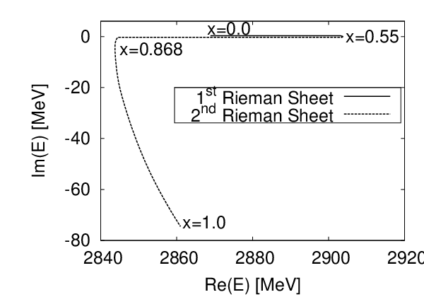
The breaking of the SU(3) symmetry through the parameter x of Eq. (23) makes the , pole, which is member of the lightest of the triplets, first approach the threshold up to x=0.55 but, instead of crossing it at some point and becoming a resonance able to decay into this channel, it turns into a virtual state. That is, it moves into the second Riemann sheet, and stays below threshold moving away from it over the real axis. However, for values of x bigger than 0.868, it starts acquiring an imaginary part and can no longer be interpreted as a physical state. This behaviour is shown in Fig. 1, where we present a plot of the path that this pole describes while breaking the SU(3) symmetry.
This pole and its companion had already been predicted in [11]. In that work only the interaction of pseudo-scalars and baryons were considered and the states obtained there turn out to be much more bound (binding energies of about 130-250 MeV) than in the present approach. In this case, vector meson degrees of freedom play a minor role, and the origin of the discrepancy now should be traced back to our pattern of SU(4) flavour breaking, which makes our interaction weaker in this sector by a factor than that used in [11]. For the sextet there is also predictions of pentaquarks based in the Skyrme model in [22]. The masses of the states in that paper are 100 MeV lower than the ones we find with our approach.
We also show in Tables 4, 5 and 6 the couplings of the members of the anti-sextet and the two triplets to the different channels that appear in their dynamics.
| , | , | , | ||||||||||||||||||||||||||||||||||||
|---|---|---|---|---|---|---|---|---|---|---|---|---|---|---|---|---|---|---|---|---|---|---|---|---|---|---|---|---|---|---|---|---|---|---|---|---|---|---|
|
|
|
| , | ||||||||||||
|
| , | , | ||||||||||||||||||||||||||||
|---|---|---|---|---|---|---|---|---|---|---|---|---|---|---|---|---|---|---|---|---|---|---|---|---|---|---|---|---|---|
|
|
III.2 The states
The states are shown in Table 2. The situation here is similar to the case of the states. The states in the 15′-plet and the 15-plets are strongly bound while the poles in the anti-sextet and the triplet turn out to be less bound. In any case one should notice that one of the members of the heaviest 15-plet is a candidate for the claimed anti-charmed pentaquark in [8]. The pentaquark was claimed to be seen in and spectrum with a mass MeV. There is, though, controversy about the existence of this state since other experiments failed to confirm it [24]. The , pole at position MeV is basically a bound state of and has sizable couplings to and . The channel is open and is responsible for the MeV width of the resonance. The state claimed in [8] has been observed in the decay mode
| (24) |
where the has been identified from its decay first to a soft pion with a meson and the subsequent decay of the to a . Our dynamically generated state has other two possible decay channels induced by its coupling to channels involving the resonance, which is not a stable particle. Thus, the anti-charmed resonance can decay to or plus a virtual , which subsequently would decay into a pair. To take this possibility into account, we follow the prescription used in [23, 25] and convolute the loop function of the channels with the with the spectral function of this resonance:
| (25) | |||||
| (26) |
We have also changed the subtraction point in order to get the mass of this resonance closer to the claimed value of 3100 MeV. We did that by increasing 10% the value of the subtraction point. The new pole position, taking into account the 120 MeV width of the and the slightly changed subtraction point is MeV. We note though that our resonance has a much bigger width ( MeV) than the one observed experimentally ( MeV). However, our dynamically generated state has now another two decay mechanisms apart from the one in Eq. (24), namely
| (27) | |||||
| (28) |
The decay in Eq. (27) has the same particles in the final state that in Eq. (24), with the difference that the pion in one case is coming from the decay of the and therefore has low momentum, while in the other channel it comes from a and may have higher momentum. The experimental search made in [8] looked only for pions in order to reconstruct a and may have missed the other events where the pion comes from a .
Observing the Table 2, one actually sees that there are other poles with that can decay to , but their masses do not agree well with that of the observed experimental state. On the other hand, we see also that some other states from the table may be affected by the consideration of the or widths. We show in Table 7, the new pole positions of the resonances sizable affected by considering the widths of the ( =120 MeV) and (=35 MeV). For and only two states are notably affected in each case but in the case of many more states become broader because of the consideration of the decay of its unstable components.
| SU(3) Irrep | Re() | Im() | ||
|---|---|---|---|---|
| Pole [MeV] | [MeV] | [MeV] | ||
| 0 | 2 | 3114.9 | 13.8 | |
| 1 | 3/2 | 3206.6 | 2.4 | |
| 0 | 2 | 3055.7 | 19.1 | |
| 1 | 3/2 | 3187.2 | 16.9 | |
| 2 | 1 | 3324.1 | 2.5 | |
| 15 | 0 | 1 | 2964.0 | 26.0 |
| 1 | 3/2 | 3156.1 | 19.6 | |
| 15 | 0 | 1 | 3062.4 | 26.8 |
| 1 | 3/2 | 3168.7 | 3.9 | |
| 15 | 0 | 1 | 3114.9 | 13.8 |
| 3/2 | 3216.0 | 9.9 |
We can also compare here our states with previous predictions from [22]. In that paper, with the Skyrme model, a 15-plet of pentaquarks was found. The masses of the pentaquark states are between 100 and 200 MeV lower than the masses of the states belonging to the lighter 15-plet that we generate dynamically. Predictions for a negative charmed 15-plet had also been made in [12]. In that paper only the interaction of pseudo-scalar mesons with the ground state of baryons have been considered, while in the present work also the vector mesons and the baryons are taken into account. The results obtained in that paper are to be compared with the light 15-plet obtained in the present work, since this multiplet is mainly coming from the , as can be seen from Table 8 where the couplings of the states to the different channels are given. Also here the states obtained with the model are 100-200 MeV heavier (less bound) than in the previous work [12], which did not considered the heavy quark symmetry. Part of this difference comes here again because our interactions are weaker than those used in this latter reference by a factor of the order of . The couplings of the resonances can be also compared in both works. The strength of the couplings in the present approach are mostly in the channels coming from the interaction but there is a sizeable mixing with states coming from the or in some sectors. Moreover, since our states are less bound, the total amount of strength in the couplings is smaller [21] than in [12].
We also compile in Tables 9 and 10 the couplings of the resonances belonging to the anti-sextet and the triplet from Table 2. The poles of the anti-sextet are placed relatively close to threshold, where the current approach might be more appropriate, and their dynamics is mostly controlled by channels involving vector meson degrees of freedom not considered up to now. On the other hand, they are sufficiently bound (tens of MeV) to expect their existence to be guarantied under reasonable changes of the employed renormalization scheme or of the pattern of SU(8) symmetry breaking. Finally, in Table 11 we present the couplings of the poles belonging to the heaviest 15-plet of Table 2.
| , | , | , | ||||||||||||||||||||||||||||||||||||
|---|---|---|---|---|---|---|---|---|---|---|---|---|---|---|---|---|---|---|---|---|---|---|---|---|---|---|---|---|---|---|---|---|---|---|---|---|---|---|
|
|
| ||||||||||||||||||||||||||||||||||||
| , | , | , | ||||||||||||||||||||||||||||||||||||
|
|
|
| , | , | , | ||||||||||||||||||||||||||||||
|---|---|---|---|---|---|---|---|---|---|---|---|---|---|---|---|---|---|---|---|---|---|---|---|---|---|---|---|---|---|---|---|---|
|
|
|
| , | , | ||||||||||||||||||||||
|
|
| , | , | , | ||||||||||||||||||||||||||||||||||||
|---|---|---|---|---|---|---|---|---|---|---|---|---|---|---|---|---|---|---|---|---|---|---|---|---|---|---|---|---|---|---|---|---|---|---|---|---|---|---|
|
|
| ||||||||||||||||||||||||||||||||||||
| , | , | , | ||||||||||||||||||||||||||||||||||||
|
|
|
III.3 The states
The states found within our approach are shown in Table 3. There is only one possible combination of multiplets with quantum numbers which is the . From this interaction there is one attractive 15-plet. Most of the states in this sectors are bound by more than 100 MeV. Those are novel predictions from the present approach. We display in Table 12 the couplings of the generated resonances to the different channels.
| , | , | , | ||||||||||||||||
|---|---|---|---|---|---|---|---|---|---|---|---|---|---|---|---|---|---|---|
|
|
| ||||||||||||||||
| , | , | , | ||||||||||||||||
|
|
|
IV Conclusions
In this work we have analyzed the spectrum of dynamically generated resonances from the interaction of non-charmed baryons with negative charmed mesons. In order to construct the interaction we followed a model based on the symmetry that respects the heavy quark symmetry of the strong interactions in the charm sector. The large spin–flavor symmetry is actually broken by the use of physical masses for the hadrons and the decay constant of the mesons, and , instead of in the vertices.
Within the present approach we find a very rich spectrum of exotic baryons with negative charm quantum number. Such states cannot be constructed in the usual interpretation for the baryons whose structure should be made of three quarks. With we find 6 multiplets of resonances, namely a -plet, two 15-plets, an anti-sextet and two triplets. For our model generates 5 multiplets, a -plet, two 15-plets, an anti-sextet and a triplet. Finally for the model generates a single 15-plet.
The results of the present approach were compared with previous works. The model generates the multiplets that had already been predicted in [11, 12, 22], and the states obtained here are around 100-200 MeV heavier than the exotic states obtained in previous works. In addition, the model generates new multiplets on top of the ones predicted before. This is a consequence of the inclusion of many more channels, as required to enforce the heavy quark symmetry in the charm sector.
There has been one experimental claim for an anti-charmed baryon in [8]. One of the dynamically generated states found within the present approach could be a candidate for the anti-charmed baryon experimentally claimed in [8], although with a larger width. In this case, we have also shown that there could be other decay channels competing with the one analyzed in [8].
Acknowledgments
This work is partly supported by DGI and FEDER funds, under contract FIS2006-03438, FIS2008-01143/FIS and PIE-CSIC 200850I238 and the Junta de Andalucia grant no. FQM225. We acknowledge the support of the European Community-Research Infrastructure Integrating Activity ”Study of Strongly Interacting Matter” (acronym HadronPhysics2, Grant Agreement n. 227431) under the Seventh Framework Programme of EU. Work supported in part by DFG (SFB/TR 16, ”Subnuclear Structure of Matter”). L.T. acknowledges support from the RFF program of the University of Groningen.
References
- [1] M. Artuso et al. [CLEO Collaboration], Phys. Rev. Lett. 86, 4479 (2001) [arXiv:hep-ex/0010080].
- [2] R. Mizuk et al. [Belle Collaboration], Phys. Rev. Lett. 94, 122002 (2005) [arXiv:hep-ex/0412069].
- [3] C. P. Jessop et al. [CLEO Collaboration], Phys. Rev. Lett. 82, 492 (1999) [arXiv:hep-ex/9810036].
- [4] S. E. Csorna et al. [CLEO Collaboration], Phys. Rev. Lett. 86, 4243 (2001) [arXiv:hep-ex/0012020].
- [5] R. Chistov et al. [BELLE Collaboration], Phys. Rev. Lett. 97, 162001 (2006) [arXiv:hep-ex/0606051].
- [6] T. Amirzadeh et al. [Birmingham-CERN-Glasgow-Michigan State-Paris Collaboration and Cambridge-Mi], Phys. Lett. B 89, 125 (1979).
- [7] V. M. Karnaukhov, V. I. Moroz, C. Coca and A. Mihul, Phys. Lett. B 281, 148 (1992).
- [8] A. Aktas et al. [H1 Collaboration], Phys. Lett. B 588, 17 (2004) [arXiv:hep-ex/0403017].
- [9] M. F. M. Lutz and E. E. Kolomeitsev, Nucl. Phys. A 730, 110 (2004) [arXiv:hep-ph/0307233].
- [10] C. E. Jimenez-Tejero, A. Ramos and I. Vidana, Phys. Rev. C 80, 055206 (2009) [arXiv:0907.5316 [hep-ph]].
- [11] J. Hofmann and M. F. M. Lutz, Nucl. Phys. A 763, 90 (2005) [arXiv:hep-ph/0507071].
- [12] J. Hofmann and M. F. M. Lutz, Nucl. Phys. A 776, 17 (2006) [arXiv:hep-ph/0601249].
- [13] J. Haidenbauer, G. Krein, U. G. Meissner and A. Sibirtsev, Eur. Phys. J. A 33 (2007) 107 [arXiv:0704.3668 [nucl-th]].
- [14] C. Garcia-Recio, V. K. Magas, T. Mizutani, J. Nieves, A. Ramos, L. L. Salcedo and L. Tolos, Phys. Rev. D 79, 054004 (2009) [arXiv:0807.2969 [hep-ph]].
- [15] C. Garcia-Recio, J. Nieves and L. L. Salcedo, Phys. Rev. D 74, 036004 (2006) [arXiv:hep-ph/0605059].
- [16] C. Garcia-Recio, J. Nieves and L. L. Salcedo, Phys. Rev. D 74, 034025 (2006) [arXiv:hep-ph/0505233].
- [17] H. Toki, C. Garcia-Recio and J. Nieves, Phys. Rev. D 77 (2008) 034001 [arXiv:0711.3536 [hep-ph]].
- [18] J. Nieves and E. Ruiz Arriola, Phys. Rev. D 64, 116008 (2001) [arXiv:hep-ph/0104307].
- [19] L. Roca, E. Oset and J. Singh, Phys. Rev. D 72, 014002 (2005) [arXiv:hep-ph/0503273].
- [20] D. Gamermann, E. Oset, D. Strottman and M. J. Vicente Vacas, Phys. Rev. D 76, 074016 (2007) [arXiv:hep-ph/0612179].
- [21] D. Gamermann, J. Nieves, E. Oset and E. R. Arriola, Phys. Rev. D 81 (2010) 014029 arXiv:1001.3254 [hep-ph].
- [22] B. Wu and B. Q. Ma, Phys. Rev. D 70, 034025 (2004) [arXiv:hep-ph/0402244].
- [23] L. Roca, S. Sarkar, V. K. Magas and E. Oset, Phys. Rev. C 73, 045208 (2006) [arXiv:hep-ph/0603222].
- [24] B. Aubert et al. [BABAR Collaboration], Phys. Rev. D 73, 091101 (2006) [arXiv:hep-ex/0604006].
- [25] D. Gamermann and E. Oset, Eur. Phys. J. A 33, 119 (2007) [arXiv:0704.2314 [hep-ph]].