Radiative contribution to neutrino masses and mixing in SSM
Abstract:
In an extension of the minimal supersymmetric standard model (popularly known as the SSM), three right handed neutrino superfields are introduced to solve the -problem and to accommodate the non-vanishing neutrino masses and mixing. Neutrino masses at the tree level are generated through parity violation and seesaw mechanism. We have analyzed the full effect of one-loop contributions to the neutrino mass matrix. We show that the current three flavour global neutrino data can be accommodated in the SSM, for both the tree level and one-loop corrected analyses. We find that it is relatively easier to accommodate the normal hierarchical mass pattern compared to the inverted hierarchical or quasi-degenerate case, when one-loop corrections are included.
Keywords:
Beyond Standard Model, Neutrino Physics, Supersymmetric Standard Model1 Introduction
Despite its stupendous success in explaining elementary particle interactions, the celebrated standard model (SM) of particle physics suffers from some shortcomings, both theoretical and experimental. On the experimental side, explaining the masses and the mixing pattern of neutrinos is a task in which the SM is an apparent failure. The neutrino sector, therefore, is a natural testing ground for most proposals for going beyond the SM.
Supersymmetry (SUSY) is a rather popular choice for new physics. The minimal supersymmetric version of the SM (MSSM) provides a natural solution to the so-called “gauge-hierarchy problem” through the introduction of superpartners of SM-particles. However, MSSM itself is not free of drawbacks. One of these is the so-called -problem [1], which essentially means our lack of understanding as to why the higgsino mass parameter, a SUSY invariant quantity, has to be around the SUSY breaking scale. This problem can be solved in the next-to minimal supersymmetric version of the standard model (NMSSM), where, unlike in the MSSM, the -term becomes a derived quantity with the right order of magnitude.
Unfortunately, neither the MSSM nor NMSSM by itself can explain the observed pattern of neutrino masses and mixing, on which definite guidelines have been set down by existing data [2, 3]. The situation becomes different if one allows violation of the discrete symmetry known as -parity () [4, 5, 6, 7, 8, 9, 10, 11, 12], defined as , where is the lepton(baryon) number and is the spin, of a particle. Neutrino masses and mixing have been analyzed in these models under various assumptions, both at the tree level and by taking loop-induced effects into account. Neutrino mass generation in variants of violating MSSM have been addressed in refs. [13, 14, 15, 16, 18, 17, 19, 20, 21, 22, 23, 24, 25, 26, 27, 28, 29, 30, 31, 32, 33, 34, 35, 36, 37, 38, 39, 40, 41, 42, 43, 44, 45, 46, 47, 48, 49, 50, 51, 52, 53, 54, 55, 56, 57, 58, 59, 60, 61, 62]. Such extensive study has established -violation to be as potent in neutrino mass generation as the well-known seesaw mechanism [63, 64, 65, 66, 67] which requires introduction of gauge singlet neutrino superfields.
R-parity violation, in both the contexts of accelerator phenomenology and, for example, neutrino mass generation, have been extensively studied in various scenarios, especially in its L-violating incarnation. Thus one has so-called trilinear R-parity violation driven by the or -type terms in the superpotential. In addition to new signals induced by three-body decays of the lightest neutralino, neutrino masses are generated through loop effects in such scenarios [13, 14, 15, 16, 18, 17, 19, 20]. Then one can have R-parity broken by bilinear terms [21, 22, 23, 24, 25, 26, 27, 28, 29, 30, 31, 32, 33, 34, 35, 36, 37, 38, 39, 40, 41, 42, 43, 44, 45, 46, 47, 48, 49, 50, 51, 52, 53, 54, 55, 56, 57, 58] of the type . One here notices remarkable features like (a) non-zero vacuum expectation values for sneutrinos, and (b) the mixing between neutrinos and neutralinos as well as charged leptons and charginos. Such a scenario generates one neutrino mass at the tree level while the other mass(es) need to be generated via loop effects [39, 40, 41, 42, 43, 44, 45, 46, 47, 48, 49, 50, 51]. The characteristic signal consists in final state with comparable numbers of muons and taus at high energy colliders [52, 53, 54, 55, 56, 57, 58].
Bilinear R-parity violation, is also linked with spontaneous L-breaking [10, 59, 60, 61, 62] via a singlet sneutrino vacuum expectation value (VEV). Such an effect triggers terms of the type in the superpotential, and also leaves as its footprint a Majoron which has its own experimental signature [68, 69, 70], being an additional source of missing energy.
In the backdrop of such a rich phenomenology of relatively minimalistic R-parity breaking models, further embellishments on the minimal scenarios have also been studied, often with some specific goals. A proposal for neutrino mass generation together with a solution to the -problem, with the same set of gauge-singlet right chiral neutrino superfields, has been advocated in [71]. This is popularly known as SSM. Following this proposal, the scalar sector and the parameter space of SSM was studied in great detail in [72]. In SSM, the three generations of SM-neutrinos can acquire masses through a TeV-scale seesaw mechanism, with both neutralinos and heavy neutrinos participating in the process [73]. Issues of neutrino mass generation and the -problem can also be found in some recent works [74, 75, 76, 77, 78].
A comprehensive analytical study of mass generation of light neutrinos in SSM, accompanied by necessary numerical analysis, has been discussed in ref. [73]. In this work, neutrino masses and mixing, consistent with the three flavour global neutrino data, are reproduced even with the simplistic choice of flavour diagonal neutrino Yukawa couplings . Decay modes of the lightest neutralino into two-body final states (, ) have also been considered for various compositions of the lightest neutralino. In addition, correlations between neutrino mixing angles, and ratio of the decay branching ratios into -charged lepton are studied there as a possible test of this model at the Large Hadron Collider (LHC).
Among other related studies of importance, neutrino mass generation and collider aspects of this model, with one and two generation(s) of the right handed neutrinos, have been addressed in ref.[79]. For one right handed neutrino, neutrino mass generation has been studied there upto one-loop level. Decays of the lightest neutralino into all possible final states are also studied in this reference. Constraints on complex vacuum expectation values (VEVs) from electroweak symmetry breaking (EWSB), and its consequence on the neutrino sector are studied in ref.[80], where issues concerning spontaneous CP-violation are also addressed. The role of gravitino as a dark matter candidate in this model was studied in ref.[81]. This paper also highlighted the prospects of detecting gamma rays from decaying gravitinos. For an overview of various other aspects of SSM, see the recent review [82].
In this work, we study in detail the effect of radiative corrections, upto one-loop, to the neutrino masses and mixing, consistent with the three flavour global data [2, 3]. As mentioned before, a similar study, but with just one generation of right handed neutrino, was carried out in [79]. However, a full study addressing both neutrino masses and the bilarge mixing pattern, with a complete set of one-loop corrections with all three generations of left and right handed neutrinos, has so far been lacking. This is exactly what we attempt in the present work. We also perform a systematic study to identify the crucial parameters of the model, which control the tree level or the one-loop dominance in the neutrino sector.
As shown in Ref.[73, 79], a very attractive feature of this model is that the ratios of certain decay branching ratios show very nice correlation with the neutrino mixing angles. This is very similar to bilinear R-parity violating models [52, 53, 56]. Nevertheless, one should note certain differences in these two cases. In SSM lepton number is broken explicitly in the superpotential by terms which are trilinear as well as linear in singlet neutrino superfields. In addition to that there are lepton number conserving terms involving the singlet neutrino superfields with dimensionless neutrino Yukawa couplings. After the electroweak symmetry breaking these terms can generate the effective bilinear R-parity violating terms as well as the =2 Majorana mass terms for the singlet neutrinos in the superpotential. In general, there are corresponding soft supersymmetry breaking terms in the scalar potential. Thus the parameter space of this model is much larger compared to the bilinear R-parity violating model. Hence, in general, one would not expect a very tight correlation between the neutrino mixing angles and the ratios of decay branching ratios of the LSP. However, under certain simplifying assumptions (as discussed in Sec. 3.2), one can reduce the number of free parameters and in those cases it is possible that the above correlations reappear. As mentioned earlier, this has been studied in great detail for the two body final states in [73] and for all possible two and three body final states in [79]. Let us note in passing that such a nice correlation is lost in the general scenario of bilinear-plus-trilinear R-parity violation [53].
Another important difference between SSM and the bilinear R-parity violating model in the context of the decay of the LSP (assumed to be the lightest neutralino in this case) is that in SSM the lightest neutralino can have a significant singlet neutrino () contribution. In this case, the correlation between neutrino mixing angles and decay branching ratios of the LSP is different [73, 79] compared to the cases when the dominant component of the LSP is either a bino, or a higgsino or a Wino. This gives us a possibility of distinguishing between different R-parity violating models through the observation of the decay branching ratios of the LSP in collider experiments [73, 79]. In addition, the decay of the lightest neutralino will show displaced vertices in collider experiments and when the lightest neutralino is predominantly a singlet neutrino, the decay length can be of the order of several meters for a lightest neutralino mass in the neighbourhood of 50 GeV [79]. This is very different from the bilinear R-parity violating model where for a Bino LSP of similar mass the decay length is less than or of the order of a meter or so [56].
The paper is organized as follows. We start with a brief introduction to the model in section 2 and discuss the electroweak symmetry breaking conditions. The neutrino sector is discussed in section 3 in details, accompanied with necessary analytical results. We discuss the observed pattern of neutrino masses and mixing upto one-loop corrections. We present a comprehensive discussion on the results of our numerical analysis of neutrino masses and mixing in section 4. The three broad scenarios, namely, normal hierarchy, inverted hierarchy, and quasi-degenerate neutrinos, are taken up in turn in this section. We conclude in section 5. Various technical details, such as different mass matrices, couplings, Feynman rules and the expressions for one-loop contributions are relegated to the appendices.
2 Electroweak symmetry breaking in SSM
The superpotential for SSM includes three gauge-singlet right handed neutrino superfields ( ()) along with the usual MSSM superfields. The superpotential of SSM along the lines of ref.[71] is
| (1) | |||||
where and are the Higgs superfields that have Yukawa couplings with down- and up-type quarks, respectively. are doublet quark superfields, () are singlet up-type (down-type) quark superfields, are doublet lepton superfields, and are singlet charged lepton superfields. The absence of any bilinear terms in the superpotential is ensured by imposing a symmetry (which is also used in case of NMSSM). The effective -term is given by , where is the VEV obtained by the ‘’-th right handed sneutrino (scalar component of ) after EWSB. The characteristic bilinear violating terms () appear in a similar way after the EWSB. These terms are given by . The last two terms of the superpotential (see eq.(1)) violate through L-violation. The last term, with the coefficient , is included in order to avoid an unacceptable axion associated to the breaking of a global symmetry [83]. This term generates effective Majorana masses for the singlet neutrinos at the electroweak scale.
It has been shown earlier [71, 72, 73] that the above -violating superpotential (see eq.(1)) provides the minimal structure, sufficient for both generating a neutrino mass pattern, and offering a solution to the -problem. There have been studies [84, 85] on -violating scenarios including right handed neutrinos, which use a subset of this minimal superpotential, but without any attempt to address the -problem. Similar remarks apply to earlier works [86] aimed at explaining the baryon asymmetry of the universe through leptogenesis, using the term .
The frequently discussed trilinear -violating terms, driven by the well-known - and -type couplings, need not appear explicitly in this model. The reason is the following; the above superpotential, as has already been stated, can lead to ‘bilinear’ terms of the form once the right sneutrinos acquire VEV, and, once such terms arise, they can effectively lead to the and -type terms [30, 31]. Here, as a digression, let us mention that the spontaneous breakdown of the symmetry through right-sneutrino VEV can in general lead to the formulation of domain walls [87]. The associated problems can, however, be ameliorated through well-known methods [88].
Coming back to SSM, if we confine ourselves to the framework of supergravity mediated supersymmetry breaking, the Lagrangian , containing the soft-supersymmetry-breaking terms is given by
| (2) | |||||
The first two lines of eq.(2) consist of squared-mass terms of squarks, sleptons and Higgses, the next two lines contain the trilinear scalar couplings, while in the last line, , and represent the Majorana masses corresponding to , and gauginos , and , respectively. The tree-level scalar potential receives the usual D and F term contributions, in addition to the terms from .
We adhere to the -preserving case, so that only the real parts of the neutral scalar fields develop, in general, the following VEVs,
| (3) |
The tree level neutral scalar potential looks like
| (4) | |||||
It is important to notice that the potential is bounded from below as the coefficients of the fourth power of all the eight superfields are positive. We further assume that all the parameters present in the scalar potential are real. From eq.(4), the minimization conditions in terms of can be derived (the equations are provided in appendix A). The minimization conditions for SSM have also been addressed in [72, 73, 79] . Similar conditions, but for complex VEVs, have been discussed in ref.[80]. Note that in order to generate correct order of magnitudes for the light neutrino masses through the TeV scale seesaw mechanism, one requires smaller values for neutrino Yukawa couplings and left handed sneutrino VEVs ).
3 The neutrino sector
3.1 Neutral fermions
In this model, three doublet neutrinos () and three gauge-singlet right handed neutrinos () mix with the MSSM neutralinos (two neutral gauginos and two neutral higgsinos) due to L-violating interactions (see eq.(1)). The resulting neutralino mass matrix therefore is of dimension . The mixing among various current eigenstates are governed by the VEVs of various neutral scalar fields (namely, ). This matrix has been addressed in refs. [71, 72, 73, 79] for real VEVs, and in ref. [80] for complex VEVs.
In the weak interaction basis, defined by,
| (5) |
the neutral fermion mass term in the Lagrangian is of the form
| (6) |
where is the modified neutralino mass matrix, and is given by
| (7) |
Here, using eq.(),
| (8) |
and
| (9) |
The matrix contains the block (upper left) of MSSM neutralinos as well as a block (bottom right) of gauge-singlet neutrinos and mixing terms between them. The null block in signifies the absence of Majorana mass terms for the left handed neutrinos. The elements of contain either left handed sneutrino VEVs or Higgs VEVs multiplied by neutrino Yukawa couplings , and hence, are of much smaller magnitudes compared to the entries of . This feature ensures a seesaw-like structure of .
This symmetric matrix can be diagonalized with a unitary matrix to obtain the physical neutralino states. The mass eigenstates are defined by,
| (10) |
where satisfies
| (11) |
with the diagonal neutralino mass matrix denoted as . Seven eigenvalues of this matrix turn out to be heavy, i.e. of the order of the electroweak scale, and thus correspond to the physical neutralinos. The remaining three light eigenvalues correspond to the masses of three SM-neutrinos. One can therefore write eq.(11) alternatively as
| (12) |
where and .
Assuming small violation, it is possible to carry out a perturbative diagonalization of the neutralino mass matrix (see [89]), by defining [90] a matrix as
| (13) |
If the elements of satisfy , then this can be used as an expansion parameter to get an approximate analytical solution for the matrix (see eq.(11)). A general expression for the elements of with simplified assumptions can be written in the form , where
| (14) |
with , and are complicated functions of various parameters of the model. The complete expressions for the elements of are given in appendix B. Here we neglect the subdominant terms , , , where is the electroweak (or supersymmetry breaking) scale.
3.2 Seesaw mechanism and tree level neutrino mass
The effective light neutrino mass matrix , arising via the seesaw mechanism in presence of explicit lepton number violation, is in general given by
| (17) |
The eigenvalues and eigenvectors of the matrix were computed in ref.[73] with the simplifying assumption of a flavour diagonal structure of the neutrino Yukawa couplings . Three flavour global neutrino data were fitted with this assumption, and it was observed that all three neutrinos acquire masses even at the tree level.
An approximate analytical expression for the elements of at tree level, as obtained in ref.[73], with certain simplifying assumptions is given by
| (18) |
One can further rewrite eq.(18) in an elucidate form given by
| (19) |
where and are given by eq.(14) and
| (20) |
with
| (21) |
The reason for recasting eq.(18) in terms of and becomes clear when we will discuss our numerical results in section 4. In , we neglect the subdominant terms of the order of , and . For the convenience of the reader, let us also mention here that we choose , , , and all soft masses to be flavour diagonal and flavour blind, The neutrino Yukawa couplings () and the corresponding soft terms are, however, chosen to be flavour diagonal.
3.3 One loop corrections to the self energies
In the regime of renormalizable quantum field theories, stability of any tree level analysis must be re-examined in the light of radiative corrections. Following this prescription, the results of neutrino masses and mixing will be more robust, once tree level analysis is further improved by incorporating radiative corrections. The radiative corrections may have sizable effect on the neutrino data at one-loop level. Thus, although all three SM neutrinos acquire non-zero masses in the SSM even at the tree level [73], it is interesting to investigate the fate of those tree level masses and mixing when exposed to one-loop corrections. With this in view, in this section we perform a systematic study of the neutrino mass and mixing with all possible one-loop corrections both analytically and numerically. In the subsequent sections, while showing the results of one-loop corrections, we try to explain the deviations (which may or may not be prominent) from the tree level analysis. The complete set of one-loop diagrams are shown in figure1. Before going into the details, let us discuss certain relevant issues of one-loop correction and renormalization for the neutralino-neutrino sector. The most general one-loop contribution to the unrenormalized neutralino-neutrino two-point function can be expressed as
| (22) |
where and are defined in eq.(109), and is the external momentum. The unrenormalized self-energies and depend on the squared external momentum . The generic self energies of the (Majorana) neutrino must be symmetric in its indices . The resulting one-loop corrected mass matrix using dimensional reduction () scheme [91] is given by
| (23) |
with
| (24) |
where the tree level neutralino mass is defined at the renormalization scale , set at the electroweak scale. Here, the word neutralino mass stands for all the ten eigenvalues of the neutralino mass matrix. The self-energies are also renormalized in the scheme [91] and denoted by and respectively. The detailed expressions of and are given in appendix F.
3.4 Radiative corrections to neutrino mass terms
In this section we consider the effect of radiative corrections to the light neutrino masses. Let us recapitulate some of the earlier work regarding one-loop corrections to the neutralino-neutrino sector. The complete set of radiative corrections to the neutralino mass matrix in the conserving MSSM was discussed in ref.[92], and the leading order neutrino masses has been derived in ref.[6]. One-loop radiative corrections to the neutrino-neutralino mass matrix in the context of a -violating model were calculated in ref.[25] using ’t-Hooft-Feynman gauge. In ref.[42], gauge has been used to compute the corrections to the neutrino-neutralino mass matrix at one-loop level in an -violating scenario. Neutrino mass generation at the one-loop level in other variants of -violating MSSM has also been addressed in refs. [39, 40, 50, 44, 45, 46, 47, 48, 19, 49, 51, 84, 99].
We begin by outlining the strategy of our analysis. We start with a general neutralino matrix, with off-diagonal entries as well, which has a seesaw structure in the flavour-basis (see eq.(7)). Schematically, we can rewrite eq.(7) as,
| (25) |
where the orders of the block matrices are as those indicated in eq.(7), and the subscript ‘’ denotes the flavour basis. Here stands for the Majorana mass matrix of the heavy states, while contains the Dirac type masses for the left handed neutrinos. In the next step, instead of utilising the seesaw structure of this matrix to generate the effective light neutrino mass matrix for the three active light neutrino species, we diagonalize the entire matrix . The diagonal matrix thus contains tree level neutralino masses, which we symbolically write as
| (26) |
where are the masses of the heavy states (left handed neutrinos). At this stage we turn on all possible one-loop interactions, so that the matrix picks up radiatively generated entries, both diagonal and off-diagonal. The resulting one-loop corrected Lagrangian for the neutralino mass terms, following eq.(6), can be written as
| (27) |
where contains the effect of one-loop corrections. The matrix is diagonal, but the matrix is a general symmetric matrix with off diagonal entries.
One can rewrite the above equation, using eqs.(10 and 11), as
| (28) |
This is nothing but the one-loop corrected neutralino mass term in the Lagrangian in the flavour basis. Symbolically,
| (29) |
with the matrix having the form
| (30) |
The quantities and stand for one-loop corrections to the heavy neutralino states and light neutrino states respectively, in the flavour basis . The entity arises because of the off diagonal interactions, i.e. between the heavy neutralinos and the light neutrinos, in the same basis. Note that all of , , in the basis are given by the second term on the right hand side of eq.(23). We suitably transform them into the basis with the help of neutralino mixing matrix . Interestingly, the matrix once again possesses a seesaw structure, and one can therefore write down the one-loop corrected effective light neutrino mass matrix as
| (31) |
Let us now present an approximate form of eq.(31). For simplicity, let us begin by assuming the quantities present in eq.(31) to be c-numbers (not matrices). In addition, assume (justified later), so that eq.(31) may be written as,
| (32) |
with . Now, even when and , eq.(32) looks like
| (33) |
Thus, up to a very good approximation one can rewrite eq.(33) as
| (34) |
Reimposing the matrix structure and using eq.(17), eq.(34) can be modified as,
| (35) |
The eigenvalues of the one-loop corrected neutrino mass matrix thus correspond to one-loop corrected light neutrino masses. In conclusion, it is legitimate to calculate one-loop corrections to the light neutrino mass matrix only, and diagonalize it to get the corresponding one-loop corrected mass eigenvalues.
Let us denote the one-loop corrections to the masses of heavy neutralinos and light neutrinos in the basis by and respectively. The one-loop corrections arising from neutralino-neutrino interactions is denoted by in the same basis. The tree level neutralino mixing matrix can then be written as,
| (36) |
where the entries of the matrices are , due to very small neutrino-neutralino mixing [93]. The quantities and represent the Dirac mass of neutrino and the Majorana mass of neutralino. From eq.(28), it is easy to figure out the relation between and as,
| (37) |
Typically, for a Dirac neutrino, the mass is , while for a neutralino, the mass is . This means that the entries of the off-diagonal blocks in eq.(36) are . Therefore, for all practical purposes, one can neglect the first three terms in comparison to the fourth term on the right hand side of eq.(37). Thus,
| (38) |
up to a very good approximation. With this in view, our strategy is to compute the one-loop corrections in the basis first, and then use eq.(38) to obtain the corresponding corrections in the flavour basis. Finally, we diagonalize eq.(35) to obtain the one-loop corrected neutrino masses. We have performed all calculations in the ’t-Hooft-Feynman gauge. Let us also note in passing that the form of eq.(23) predicts off-diagonal entries (). The off-diagonal elements are responsible for the mixing between diagonal entries, they become dominant only when , and then, one can choose for external momentum[25]. Thus, one can conclude that unless the tree level masses are degenerate, the off-diagonal radiative corrections can be neglected for all practical purposes, when at least one index or refers to a heavy states.
The self-energy corrections contain entries of the neutralino mixing matrix through the couplings (see, appendix E). This is because, the self energies and in general contain products of couplings of the form . The matrix , on the other hand, contains the expansion parameter in the leading order (see eq.(15)). This observation, together with the help of eq.(65), help us to express the effective structure of the one-loop corrected neutrino mass matrix as,
| (39) |
where and are given by eq.(14) and ’s are functions of our model parameters and the Passarino-Veltman functions [94, 95, 96] defined in appendix G. The form of the loop corrected mass matrix thus obtained is identical to the tree level one (see, eq.(19)) with different coefficients , and arising now.
Note that the one-loop diagrams in figure1, contributing to the neutrino mass matrix are very similar to those obtained in bilinear R-parity violating scenario [42, 43, 44, 45, 50, 51]. However, it has been pointed out in Ref.[79], that there is a new significant contribution coming from the loops containing the neutral scalar and pseudoscalar with dominant singlet component. This contribution is proportional to the mass-splitting between the singlet scalar and pseudoscalar states [97, 98, 99]. The corresponding mass splittings for the doublet sneutrinos are much smaller [79].


3.5 Neutrino mixing
The unitary matrix which diagonalizes the light neutrino mass matrix, can be parametrized as [100],
provided the charged lepton sector is in the mass-basis (see appendix D). Here , , and all violating phases (Dirac or Majorana) are set to zero. The experimental data on neutrino oscillations [101, 102] indicate that a bilarge pattern of mixing of neutrinos may be preferred, which means that two of the mixing angles must be large. As a first approximation, one can work with , and , which is often referred to as the ‘tribimaximal structure’ [103]. Following the above discussions, we can write down the tree level PMNS matrix as,
| (46) |
where is the matrix that diagonalizes the tree level mass matrix (eq.(17)).
Similarly, the unitary matrix that diagonalizes the one-loop corrected neutrino mass matrix (eq.(35)), can be denoted as . Symbolically
| (47) |
with , , as the three one-loop corrected light neutrino masses. A similar relation for the tree level calculation is given by the second equation of (3.1), with ’s as the tree level neutrino masses.
When we include one-loop corrections, the PMNS matrix is defined as
| (48) |
where is the matrix which diagonalizes the one-loop corrected mass matrix . The scheme for obtaining the loop-corrected neutrino mixing matrix is shown in figure2.

4 Numerical results of neutrino mass and mixing
In this section we present and explain the results of our numerical analysis. Let us begin with a brief outline of the different well known schemes of light neutrino masses as favoured by experiments. These are (i) The normal hierarchy: , , (ii) The inverted hierarchy: , and (iii) The quasi-degenerate pattern: , where , and are the three light neutrino masses. Here, and for Normal (inverted) Hierarchy. The possibility of more than one scheme of neutrino masses essentially stems from our lack of knowledge of the signs of the squared mass differences, or the value of individual masses. Such being the case, the numerical analysis must be subjected to address all the three probable schemes.
The numerical calculations have been performed with the help of a code developed by us in Fortran and the results have been cross-checked using another Mathematica [104] based program we developed. In the code, we keep the left handed sneutrino VEVs (), the right handed sneutrino VEVs and the neutrino Yukawa couplings as free input variables, and then scan over the parameter space for a region consistent with the three flavour global neutrino data. For all our numerical analysis we keep the right handed sneutrino VEVs fixed at some chosen values (see table 1). The only exception to this is when we study the correlation of neutrino data with the bilinear -violating parameter . For that particular study, we vary the right handed sneutrino VEVs (consistent with EWSB conditions) within the mass scale – to –. The table 1 shows our choice of the sample parameters for the numerical analysis. The relation between the gaugino soft masses and are assumed to be GUT (grand unified theory) motivated, so that, at the electroweak scale, we have . We choose .
| tan | |||||||
|---|---|---|---|---|---|---|---|
| 10 | 0.10 | 0.45 |
We scanned the parameter space comprising of the left handed sneutrino VEVs and the neutrino Yukawa couplings extensively and found certain ranges of these parameters appropriate for various hierarchical schemes of the light neutrino masses. In table 2, some sample values for these six parameters for the different mass schemes of neutrinos are given. These values are just for illustration and the parameters were scanned around these numbers to generate the plots shown in this section. The other relevant parameters have values as mentioned in table 1.
| Normal hierarchy | 3.550 | 5.400 | 1.650 | 0.730 | 10.100 | 12.450 |
| Inverted hierarchy | 12.800 | 3.300 | 4.450 | 8.350 | 8.680 | 6.400 |
While fitting the three flavour global neutrino data, we consider constraints arising from the oscillation data as well as from the non-oscillation data. We probe the effects of these constraints for both tree level and (tree + one-loop) level analyses. The oscillation data constrain the solar and atmospheric mass squared differences, namely, and , and three neutrino mixing angles . The present 3 limits are [2, 3],
The non-oscillation constraints follow from experiments like decay [105, 106, 107], neutrinoless double beta decay [108, 109, 110] (this is also sensitive to Majorana nature and phases), and from cosmology [111]. Here we set all the Majorana phases to be zero, as we are dealing with a preserving situation.
The set of non-oscillation constraints are given as,
where s are three light neutrino masses, and s are the elements of the first row of the neutrino mixing matrix (see eq.(3.5)).
4.1 Normal hierarchy
In the normal hierarchical pattern of the three light neutrino masses, the atmospheric and the solar mass squared differences, given by and , are largely governed by the higher mass squared in each case, namely, and , respectively. Before going into the discussion of the variation of the mass-squared values with the model parameter, some general remarks are in order. First of all, note that in eq.(14), if we choose such that , then [80]. Thus, for large , we remind ourselves that in eq.(18), the effective light neutrino mass matrix has two types of seesaw structures [73]. The first one is the ordinary seesaw, given by
| (51) |
where represents the Dirac mass term for neutrinos, and stands for the Majorana mass term of the right handed neutrino. The second type is called the gaugino seesaw, in which the role of the Dirac mass terms are played by and , where are the and the gauge couplings respectively and stands for the left handed sneutrino VEV . The role of the Majorana masses are played by the gaugino soft masses . This seesaw relation is given as
| (52) | |||||
where the subscript ‘’ and is the reduced gaugino mass defined by
| (53) |
here plays the role of the effective heavy mass provided by the neutral electroweak gaugino sector, and the effect is closely analogous to Type-III seesaw mechanism[112]11 1 We thank Anjan Joshipura for pointing this out to one of the authors in a private discussion.. As discussed after eq.(39), when one-loop corrections are added, the neutrino masses are still determined by the quantities and ( for large ).


In the subsequent plots, we show the variation of the neutrino squared masses () and the atmospheric and solar mass squared differences with the square of the seesaw parameters and . Results are shown for the tree level as well as the one-loop corrected neutrino masses. These plots also demonstrate the importance of one-loop corrections to neutrino masses compared to the tree level results.
Typical mass spectra are shown in figure 3. Note that a particular model parameter has been varied while the others are fixed at values given in tables 1 and 2. The effective light neutrino mass matrix given in eq.(18) suggests that as long as and , the second term on the right hand side of eq.(18) dominates over the first term and as a result the heaviest neutrino mass scale () is controlled mainly by the gaugino seesaw effect. This is because in this limit , and, as discussed earlier, a neutrino mass matrix with a structure can produce only one non-zero neutrino mass. This feature is evident in figure3, where we see that increases as a function of . The other two masses are almost insensitive to . A mild variation to comes from the combined effect of gaugino and ordinary seesaw. On the other hand, the two lighter neutrino mass scales ( and ) are controlled predominantly by the ordinary seesaw parameters . This behaviour is observed in the right panel figures of figure3. The heaviest neutrino mass scale is not much affected by the quantities .
One can also see from these plots that the inclusion of one-loop corrections, for the chosen values of the soft SUSY breaking parameters, reduces the values of and , while increasing the value of only mildly. This is because, with such a choice, the one-loop corrections cause partial cancellation in the generation of and . For the heaviest state, it is just the opposite, since the diagonalization of the tree-level mass matrix already yields a negative mass eigenvalue, on which the loop correction has an additive effect. If, with all other parameters fixed, the signs of and are reversed (leading to a positive in the place of a negative one), , and are all found to decrease through loop corrections. A flip in the sign of and the corresponding soft breaking terms, on the other hand, causes a rise in all the mass eigenvalues, notably for and .
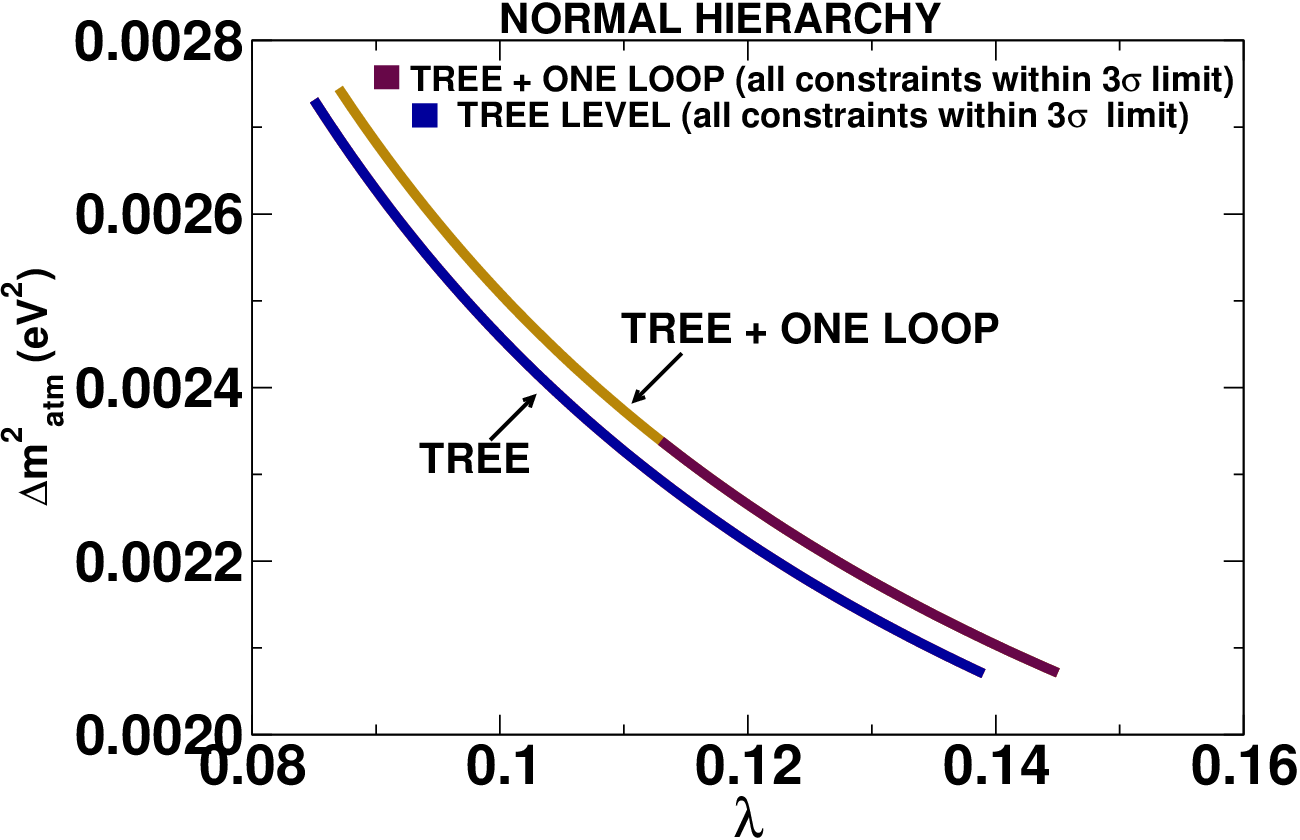
In the light of the discussion above, we now turn to explain the variation of and with and shown in figure4 and figure5. For our numerical analysis, in order to set the scale of the normal hierarchical spectrum, we choose . The left panel in figure4 shows that increases more rapidly with , whereas the variation with is much slower as expected from figure3. Similar behaviour is shown for the one-loop corrected . The small increase in the one-loop corrected result compared to the tree level one is essentially due to the splitting in value as shown earlier. The variation of with can be explained in a similar manner. Obviously, in this case the one-loop corrected result is smaller compared to the tree level one (see, figure3). However, one should note that falls off with as opposed to the variation with respect to the other two gaugino seesaw parameters. This is due to the fact that slightly decreases with but show a slow increase with respect to and . The dark solid lines in all these figures show the allowed values of various parameters where all the neutrino mass and mixing constraints are satisfied.


The variation of and with in figure5 can be understood in a similar way by looking at the right panel plots of figure3. shows a very little increase with as expected, whereas the change is more rapid with for the range of values considered along the x-axis. As in the case of figure4, the solid dark lines correspond to the allowed values of parameters where all the neutrino mass and mixing constraints are satisfied.
For higher values of , increases very slowly with these parameters (see, figure3) and this is reflected in the right panel plots of figure5, where shows a very slow variation with . On the other hand, increases more rapidly with , giving rise to a faster variation of . The plots of figure5 show that larger values of Yukawa couplings are required in order to satisfy the global three flavour neutrino data, when one considers one-loop corrected neutrino mass matrix. However, there are allowed ranges of the parameters , where the neutrino data can be satisfied with both tree and one-loop corrected analysis.
We have also considered the variation of light neutrino mass squared differences with the effective bilinear violating parameter, . For this particular numerical study we vary both and the right handed sneutrino VEVs simultaneously, in the suitable ranges around the values given in table 1 and 2. is found to increase with , whereas the solar mass squared difference decreases with increasing . The allowed region for the solar and atmospheric mass squared differences were obtained for the lower values of s. In addition, we have noticed that the correlations of with is sharper compared to the correlations seen in the case of .
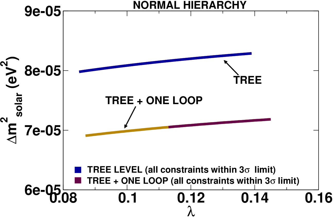
Next let us discuss the dependence of and on two specific model parameters, and , consistent with EWSB conditions. The loop corrections shift the allowed ranges of to lower values with some amount of overlap with the tree level result. On the other hand, the allowed ranges of shrinks towards higher values when one-loop corrections are included. These results are shown in figure6. We note in passing that the mass of the lightest CP-even scalar decreases with increasing . For example, can produce a lightest scalar mass of , for suitable choices of other parameters. This happens because with increasing , the lightest scalar state picks up more and more right handed sneutrino admixture.


Finally, we will discuss the dependence of and . These plots are shown in figure 7. The quantity decreases with the increasing values of and nearly saturates for larger values of . However, the one-loop corrected result for is not much different from that at the tree level for a particular value of . On the other hand, the solar mass squared difference initially increases with and for higher values of the variation slows down and tends to saturate. The one-loop corrections result in lower values of for a particular . The darker and bigger points on both the plots of figure7 are the allowed values of , where all the neutrino experimental data are satisfied. Note that only a very small range of ( 10–14) is allowed. This is a very important observation of this analysis.


Next we will discuss the light neutrino mixing and the effect of one-loop corrections on the mixing angles. It was shown in ref.[73] that for the normal hierarchical pattern of neutrino masses, when the parameter , the neutrino mixing angles and can be written as (with the tree level analysis),
| (54) |
and
| (55) |
On the other hand, the mixing angle is a much more complicated function of the parameters and and we do not show it here. Now, when , we can easily see from eq.(14), that
| (56) |
This implies that for 1 (recall that the allowed range of is 10–14),
| (57) |
As we have discussed earlier, for such values of , the quantities . Hence, the mixing angles and can be approximately written as
| (58) |
and
| (59) |
Naively, one would also expect that should show some correlation with the quantity . However, as mentioned earlier, this is a very simple minded expectation since has a more complicated dependence on the model parameters.
The variation of all three mixing angles with the corresponding parameters are shown in figure8. Note that in order to generate these plots, we vary only the quantities and all the other parameters are fixed at the values given in tables 1 and 2. We have chosen the range of parameters in such a way that the 3-flavour global neutrino data are satisfied. The mixing angles have been calculated numerically by diagonalizing the neutrino mass matrix in eq.(18) and in eq.(39). As expected from our approximate analytical expressions, these plots show very nice correlations of the mixing angles and with the relevant parameters as discussed in eqs.(58) and (59). For example, note that when , is predicted to be 0.5 and that is what we observe in the tree level plot in figure8. However, when one-loop corrections are considered, the value of is predicted to be somewhat on the lower side of the 3 allowed region. This can be understood by looking at the left panel plots of figure4, where one can see that the one-loop corrected results prefer lower values of and higher values of . Obviously, this gives smaller . On the other hand, the tree level analysis prefers higher values of and both lower and higher values of . This gives rise to large as well as small values of .


If one looks at the plot of in figure 8, then it is evident that the amount flavour in the heaviest state decreases a little bit with the inclusion of one-loop corrections for a fixed value of the quantity . Very small demands . This feature is also consistent with the plots in figure4. The correlation of with the ratio is not very sharp as expected from the discussion given above. However, a large mixing angle requires a larger value of this ratio. The effect of one-loop correction is more pronounced in this case and predicts a smaller value of compared to the tree level result. There is no specific correlation of the mixing angles with the quantities and we do not show them here.
4.2 Inverted hierarchy
In this subsection we perform a similar numerical analysis for the inverted hierarchical scheme of three light neutrino masses. Recall that for the inverted hierarchical pattern of light neutrino masses, the absolute values of the mass eigenvalues are such that . Thus the solar and the atmospheric mass squared differences are defined as and . In order to generate such a mass pattern, the choices of neutrino Yukawa couplings and the left-handed sneutrino VEVs are shown in table 2. However, these are just sample choices and other choices also exist as we will see during the course of this discussion. The choices of other parameters are shown in table 1. The effect of one-loop corrections to the mass eigenvalues are such that the absolute values of masses and become smaller whereas grows in magnitude. This effect of increasing the absolute value of while decreasing that of makes it extremely difficult to account for the present 3 limits on .


Typical mass spectra are shown in figure 9. Once again note that a particular model parameter has been varied while the others are fixed at values given in tables 1 and 2. As it is evident from these plots, the masses and are controlled mainly by the parameters , whereas the mass is controlled by the seesaw parameters though there is a small contribution coming from as well.
Let us now turn our attention to the variation of and with and shown in figure 10 and figure 11. For our numerical analysis, we have set the scale of as . The left panel in figure 10 shows that increases with and decreases with . This is essentially the behaviour shown by with the variation of . Similar behaviour is obtained for the one-loop corrected . The decrease in the one-loop corrected result compared to the tree level one is due to the splitting in value as shown in figure9.


The variation of with can be understood in a similar manner by looking at figure9. As explained earlier, in the case of , the one-loop corrected result is larger compared to the tree level one. The range of parameters satisfying all the three flavour global neutrino data are shown by the fewer dark points on the plots. Note that the increase of at the one-loop level is such that we do not even see any allowed range of parameters when looking at the variation with respect to . Once again, the behaviour of and with the change in the parameters (shown in figure11) can be explained by looking at the right panel plots of figure9.


We have also investigated the nature of variation of and with , the squared effective bilinear -violating parameters. was found to increase with (the increase is sharper for ), whereas initially increases very sharply with (particularly for and ) and then becomes flat. In the one-loop corrected results we do not find any range of values for parameters where the neutrino data are satisfied.
The variation of mass squared differences with and have also been analyzed. The variation of and with and are found to be opposite to those of normal hierarchical scenario. The one-loop corrected results do not show any allowed ranges of and (for the chosen values of other parameters) where the neutrino data can be satisfied.
The dependence of and is shown in figure12. One can see from these two figures that initially increases and then starts decreasing at a value of around . On the other hand, initially decreases and then starts increasing around the same value of . Note that the one-loop corrected result for is lower than the corresponding tree level result for whereas the one-loop corrected result for is lower than the corresponding tree level result for . For the chosen values of other parameters we see that the one-loop corrected analysis does not provide any value of where the neutrino data can be satisfied.


We conclude the discussion on inverted hierarchy by addressing the dependence of neutrino mixing angles with the relevant parameters. In figure13 we show the variation of the neutrino mixing angles with the same set of parameters as chosen for the normal hierarchical scenario. We notice that for inverted hierarchy the quantity decreases with increasing which is just opposite to that of the normal hierarchy (see, figure8). Nevertheless, the correlation of with is as sharp as in the case of normal hierarchy. A similar feature is obtained for the variation with .
On the other hand, the correlations of with and and the correlations of with and are not very sharp and we do not show them here. There are allowed values of relevant parameters where all neutrino data can be satisfied. Remember that, for the plots with s, we varied all the s simultaneously, keeping the values of s fixed at the ones determined by the parameters in table 2. Similarly, for the variation of s, the quantities s were fixed. The inclusion of one-loop corrections restrict the allowed values of parameter points significantly compared to the tree level results.


4.3 Quasi-degenerate spectra
The discussion on the light neutrino mass spectrum remains incomplete without a note on the so-called “quasi-degenerate” scenario. A truly degenerate scenario of three light neutrino masses is, however, inconsistent with the oscillation data (see eq.()). Hence, the quasi-degenerate scenario of light neutrino masses is defined in such a way that in this case all the three individual neutrino masses are much larger compared to the atmospheric neutrino mass scale. Mathematically, one writes . Obviously, the oscillation data suggest that even in such a situation there must be a mild hierarchy among the degenerate neutrinos.
In this section we have shown that the huge parameter space of SSM always leaves us with enough room to accommodate quasi-degenerate spectrum. For our numerical analysis, we called a set of light neutrino masses to be quasi-degenerate if the lightest among them is greater than 0.1 eV. We choose two sets of sample parameter points which are shown in table 3 (values of other parameters are same as in table 1). For these two sets of neutrino Yukawa couplings () and the left-handed sneutrino VEVs () we observe the following patterns of light neutrino masses at the tree level
(i) Quasi-degenerate-I:
(ii) Quasi-degenerate-II:
For case (i), we have varied the parameters around the values in table 3 and identified a few extremely fine-tuned points in the parameter space where either the tree level or the one-loop corrected result is consistent with the three flavour global neutrino data. Two representative spectrum as function of and are shown in figure 14.


| Quasi-degenerate-I | 19.60 | 19.94 | 19.99 | 9.75 | 10.60 | 11.83 |
| Quasi-degenerate-II | 18.50 | 18.00 | 18.00 | 9.85 | 10.50 | 10.10 |
As mentioned earlier, one can play with the model parameters and obtain a spectrum with a different ordering of masses termed as “Quasi-degenerate-II” in table 3. However, for such an ordering of masses, we found that it was rather impossible to find any region of parameter space where the one-loop corrected result satisfies all the constraints on neutrino masses and mixing. Nevertheless, we must emphasize here that it is not a completely generic conclusion and for other choices of soft SUSY breaking and other parameters it could be possible to have a spectrum like that shown in “Quasi degenerate II” with neutrino constraints satisfied even at the one-loop level. On the other hand, there exists regions where neutrino data are satisfied at the tree level with this ordering of masses.
5 Summary and Conclusion
In this paper, we have performed a systematic study of neutrino masses and mixing in a non-minimal extension of the MSSM, known as SSM, with the complete set of one-loop radiative corrections, over and above the effects from the seesaw mechanism (of Types I and III). A set of right chiral neutrino superfields, introduced in this model provide a solution to the -problem. Lepton number is broken by one = 1 term comprising the right-chiral neutrinos and the Higgs superfields and another = 3 term involving only the right chiral neutrinos in the superpotential. The corresponding soft SUSY breaking terms in the scalar potential together with the F-term contribution from the superpotential, induce VEVs of sneutrinos of both right and left chirality. The right chiral neutrinos, together with neutralinos, are instrumental in the generation of light neutrino masses at the tree level.
In [73], where a tree-level analysis of neutrino masses and mixing was carried out, it was shown that tree level masses could be generated in this fashion for all three light neutrinos, even with a flavour diagonal structure of neutrino Yukawa couplings (). In this work we have improved the analysis with the inclusion of one-loop radiative corrections, for various patterns of light neutrino masses, namely, the normal, inverted and quasi-degenerate spectra, Attempts have been made to identify regions in the SUSY parameter space, which can accommodate the three patterns in turn. Our analysis clearly shows that the multi-dimensional parameter space of SSM leaves enough room to accommodate all the diverse mass hierarchies of the three active light neutrinos.
As a prerequisite of the loop calculation, we have derived the entire set of Feynman rules necessary for our analytical and numerical studies. The set of rules will be of immense importance, should one want to look for signatures of this model at the Large Hadron Collider (LHC), specifically through decays of the new particles of this model into SM particles. Approximate analytical forms of the entries of the expansion matrix ‘’ have also been provided including all three generations of right handed neutrinos. A handful of relations within the four-component weak and mass eigenbasis for scalar and fermion fields of SSM have also been worked out.
The correlation of neutrino mass squared differences and mixing angles with relevant model parameters, consistent with the EWSB conditions, have been studied in detail for different mass hierarchies. The allowed regions of the parameter space are found to be rather seriously affected by the one-loop contributions. We have also observed that the globally fitted neutrino data can be accommodated into the SSM for various compositions of the Lightest Supersymmetric Particle (LSP), once one starts playing with the parameters of the model. Although for the present study, we adhered to a Bino dominated LSP scheme, we numerically verified the possibility of having a light right-chiral neutrino (i.e. singlino) like LSP, compatible with neutrino data. This, by itself, is an interesting scenario in the sense that the singlino LSP offers a scope to probe the right-handed neutrino mass-scale at the LHC. It would also be interesting to perform an explicit radiative correction to the heavy neutralinos. A dedicated analysis for this is beyond the scope of this paper, and a future publication with comprehensive discussion of all these issues may be well anticipated. In conclusion, one-loop radiative corrections to the neutrino masses and mixing angles for SSM are capable of substantially altering the tree level analysis.
Acknowledgments
We thank Utpal Chattopadhyay, Debajyoti Choudhury, Debottam Das, Anindya Datta, Aseshkrishna Datta, Dilip Kumar Ghosh, Palash Baran Pal, Subhendu Rakshit and Sreerup Raychaudhuri for helpful discussions. PG would like to thank the Council of Scientific and Industrial Research, Government of India, for a Senior Research Fellowship. PD is supported through the Gottfried Wilhelm Leibniz Program by the Deutsche Forschungsgemeinschaft (DFG). The work of PD and BM was partially supported by funding available from the Department of Atomic Energy, Government of India, for the Regional Centre for Accelerator-based Particle Physics (RECAPP), Harish-Chandra Research Institute. These two authors also acknowledge the hospitality of the Department of Theoretical Physics of the Indian Association for the Cultivation of Science (IACS), while this work was in progress. PG and SR wish to thank RECAPP for hospitality during a part of the investigation. Computational work for this study was carried out using the cluster computing facility at the Department of Theoretical Physics, IACS.
Appendix A Minimization equations
The minimization equations with respect to the VEVs are given below.
| (60) |
| (61) |
| (62) |
| (63) |
where
In deriving the above equations, it has been assumed that , , , , , are all symmetric in .
Appendix B Details of expansion matrix
In this appendix the entries of the expansion matrix are given in details
| (65) |
where
| (66) |
with .
Appendix C Scalar mass squared matrices
The superpotential of the SSM violates through lepton() number violation. This allows the Higgses (having zero lepton number) to mix with the sleptons (having non-zero lepton number). Hence, the neutral (both -odd and -even) and charged Higgs mass squared matrices are enlarged to , considering all three slepton generation. The independent entries of the -odd, -even and the charged scalar mass squared matrices were derived using eqs.(62), (63), and eq.(). Details of each of these matrix elements were given in ref. [73], hence we do not repeat them here. However, we give the expressions for scalar quark (squark) mass squared matrices.
In this appendix we present the relevant details of various scalar mass squared matrices required for the Feynman rules. The scalar sector of this model have also been addressed in ref.[72, 73, 79, 80].
C.1 CP-odd neutral mass squared matrix
In the weak interaction basis , the pseudoscalar mass term in the Lagrangian is of the form
| (67) |
where is an symmetric matrix. The mass eigenvectors are defined as
| (68) |
with the diagonal mass matrix
| (69) |
C.2 CP-even neutral mass squared matrix
In the flavour basis or weak interaction basis , the scalar mass term in the Lagrangian is of the form
| (70) |
where is an symmetric matrix. The mass eigenvectors are
| (71) |
with the diagonal mass matrix
| (72) |
C.3 Charged scalar mass squared matrix
In the weak basis basis the charged scalar mass term in the Lagrangian is of the form
| (73) |
where is an symmetric matrix. The mass eigenvectors are
| (74) |
with the diagonal mass matrix
| (75) |
One of the eight eigenvalues of the CP-odd scalar and the charged scalar mass squared matrix is zero and corresponds to the neutral and the charged Goldstone boson, respectively. We reiterate that explicit expressions for the independent entries of are given in ref. [73].
C.4 Scalar quark mass squared matrix
In the weak basis, and , we get
| (76) |
where . Explicitly for up and down type squarks , using eq.() the entries are
| (77) |
and
| (78) |
For the mass eigenstate we have
| (79) |
with the diagonal mass matrix
| (80) |
Appendix D Charged fermion mass matrix
D.1 Chargino mass matrix
The lepton number violation allows mixing between the MSSM charginos with the charged leptons and thus the chargino mass matrices enhances to . The mixing between MSSM charginos and charged leptons are governed by the left handed sneutrino VEVs() and neutrino Yukawa couplings. Both of which has to be small in order to satisfy the global neutrino data, thus this violating mixing are very small. The chargino mass matrix for the SSM have been addressed in ref.[72, 73, 79]. In the weak interaction basis defined by
| (81) |
the charged fermion mass term in the Lagrangian is of the form
| (82) |
Here for simplicity we assume diagonal form of the charged Yukawa couplings. The matrix is given by (using eq.())
| (83) |
The charged fermion masses are obtained by applying a bi-unitary transformation such that
| (84) |
where and are two unitary matrices and is the diagonal matrix with non-negative entries corresponding to the physical fermion masses. The two-component mass eigenstates are defined by
| (85) |
Nevertheless, we notice that the 13, 14, and 15 elements of the chargino mass matrix (eq. (83)) are vanishing and given the orders of magnitude of various parameters, we also see that the values of the other off-diagonal entries (except for 12 and 21 elements) are very small. This indicates that the physical charged lepton eigenstates will have a very small admixture of charged higgsino and charged gaugino states. So we can very well assume (also verified numerically) that this mixing has very little effect on the mass eigenstates of the charged leptons. Thus, while writing down the neutrino mixing matrix, it will be justified to assume that one is working in the basis where the charged lepton mass matrix is already in the diagonal form.
D.2 Quark mass matrix
The mixing matrices for up and down quarks are and they are diagonalized using bi-unitary transformation. Entries of up and down quark mass matrices are given below
| (86) |
The quark mass matrices are diagonalized as follows
| (87) |
Appendix E Feynman rules
In this appendix we will study the relevant Feynman rules required for the calculations of the one-loop contributions to the neutralino masses. Some of the Feynman rules for this model have been derived in ref.[73]. Feynman rules for MSSM are given in ref.[113, 114] and in ref.[115, 116] for MSSM with singlet superfields. Feynman rules for -violating MSSM were studied in ref.[42]. The required Feynman rules are (using relations of appendix H, shown later) of the form neutralino-fermion-scalar/gauge boson and they are listed below.
Neutralino-neutralino-neutral scalar
The Lagrangian using four component spinor notation can be written as
| (88) |
where
and
| (90) |
Neutralino-neutralino-neutral pseudoscalar
The Lagrangian using four component spinor notation can be written as
| (91) |
where
and
| (93) |
Neutralino-neutralino-
The Lagrangian using four component spinor notation can be written as
| (94) |
where
| (95) |
Neutralino-chargino-charged scalar
The Lagrangian using four component spinor notation can be written as
| (96) |
where
and
| (98) |
Neutralino-chargino-
The Lagrangian using four component spinor notation can be written as
| (99) |
where
| (100) |
and
| (101) |
The factors and are the proper signs of neutralino and chargino masses [115]. They have values .
Neutralino-quark-squark
The Lagrangian using four component spinor notation can be written as
| (102) |
where
| (103) |
and
| (104) |
Appendix F The and function
In this appendix we give the detail expressions for the renormalized self energy functions and . The net result is
| (105) |
| (106) |
Detail expressions for the couplings are given in appendix E. The functions are given in appendix G. The factor appearing in front of the quark-squark loop contributions signifies three variations of quark colour.
Appendix G The and function
Appendix H Some Useful Relations
Fermionic sector
For neutralinos the following relations between mass and weak eigenstates are very useful
| (108) |
with i varies from 1 to 10 and
| (109) |
In terms of the four component spinors for charginos, the following relations between mass and weak eigenstates are very useful.
where , and i varies from 1 to 5. The last six relations are for the charge-conjugated fields.
The four component neutralino, chargino and charge conjugated chargino spinors are respectively defined as
| (118) |
where and are two component neutral and charged spinors, respectively.
Scalar sector
References
- [1] J. E. Kim and H. P. Nilles, The Mu Problem And The Strong CP Problem, Phys. Lett. B 138 (1984) 150.
- [2] See,for example,B. Kayser, Neutrino Mass, Mixing, and Flavor Change, \arXivid0804.1497 [hep-ph] and references therein.
- [3] T. Schwetz, M. Tortola and J. W. F. Valle, Three-flavour neutrino oscillation update, New. J. Phys. 10 (2008) 113011 [\arXivid0808.2016 [hep-ph]].
- [4]
P. Fayet,
Supergauge Invariant Extension Of The Higgs Mechanism And A Model For The Electron And Its
Neutrino,
Nucl. Phys. B 90 (1975) 104;
Spontaneously Broken Supersymmetric Theories Of Weak, Electromagnetic And Strong Interactions, Phys. Lett. B 69 (1977) 489;
G. R. Farrar and P. Fayet, Phenomenology Of The Production, Decay, And Detection Of New Hadronic States Associated With Supersymmetry, Phys. Lett. B 76 (1978) 575. - [5] C. S. Aulakh and R. N. Mohapatra, Neutrino As The Supersymmetric Partner Of The Majoron, Phys. Lett. B 119 (1982) 136.
- [6] L. J. Hall and M. Suzuki, Explicit R-Parity Breaking In Supersymmetric Models, Nucl. Phys. B 231 (1984) 419.
- [7]
I. H. Lee,
Lepton Number Violation In Softly Broken Supersymmetry,
Phys. Lett. B 138 (1984) 121;
I. H. Lee, Lepton Number Violation In Softly Broken Supersymmetry. 2, Nucl. Phys. B 246 (1984) 120. - [8] G. G. Ross and J. W. F. Valle, Supersymmetric Models Without R-Parity, Phys. Lett. B 151 (1985) 375.
- [9] J. R. Ellis, G. Gelmini, C. Jarlskog, G. G. Ross and J. W. F. Valle, Phenomenology Of Supersymmetry With Broken R-Parity, Phys. Lett. B 150 (1985) 142.
- [10] A. Masiero and J.W.F. Valle, A Model For Spontaneous R Parity Breaking, Phys. Lett. B 251 (1990) 273.
- [11] B. C. Allanach, A. Dedes and H. K. Dreiner, The R parity violating minimal supergravity model, Phys. Rev. D 69 (2004) 115002 [arXiv:hep-ph/0309196].
- [12]
For reviews on R-parity violation, see, e.g.,
R. Barbier et al.,
R-parity violating supersymmetry,
Phys. Rept. 420 (2005) 1 [hep-ph/0406039];
M. Chemtob, Phenomenological constraints on broken R parity symmetry in supersymmetry models, Prog. Part. Nucl. Phys. 54 (2005) 71 [hep-ph/0406029]. - [13] S. Dawson, R-Parity Breaking in Supersymmetric Theories, Nucl. Phys. B 261 (1985) 297.
- [14] S. Dimopoulos and L. J. Hall, Lepton and Baryon Number Violating Collider Signatures from Supersymmetry, Phys. Lett. B 207 (1988) 210.
- [15] R. M. Godbole, P. Roy and X. Tata, Tau signals of R-parity breaking at LEP-200, Nucl. Phys. B 401 (1993) 67 [hep-ph/9209251].
- [16] M. Drees, S. Pakvasa, X. Tata and T. ter Veldhuis, A Supersymmetric resolution of solar and atmospheric neutrino puzzles, Phys. Rev. D 57 (1998) 5335 [hep-ph/9712392].
- [17] R. Adhikari and G. Omanovic, LSND, solar and atmospheric neutrino oscillation experiments, and R-parity violating supersymmetry, Phys. Rev. D 59 (1999) 073003.
- [18] S. Rakshit, G. Bhattacharyya and A. Raychaudhuri, R-parity violating trilinear couplings and recent neutrino data, Phys. Rev. D 59 (1999) 091701 [hep-ph/9811500].
- [19] F. Borzumati and J. S. Lee, Novel constraints on Delta(L) = 1 interactions from neutrino masses, Phys. Rev. D 66 (2002) 115012 [arXiv:hep-ph/0207184].
- [20] P. Dey, A. Kundu, B. Mukhopadhyaya and S. Nandi, Two-loop neutrino masses with large R-parity violating interactions in supersymmetry, J. High Energy Phys. 12 (2008) 100 [arXiv:0808.1523].
- [21]
A. S. Joshipura and M. Nowakowski,
’Just so’ oscillations in supersymmetric standard model,
Phys. Rev. D 51 (1995) 2421 [hep-ph/9408224];
Leptonic CP violation in supersymmetric Standard Model, Phys. Rev. D 51 (1995) 5271 [hep-ph/9403349]. - [22] M. Nowakowski and A. Pilaftsis, W and Z boson interactions in supersymmetric models with explicit R-parity violation, Nucl. Phys. B 461 (1996) 19 [hep-ph/9508271].
- [23] F. Borzumati, Y. Grossman, E. Nardi and Y. Nir, Neutrino masses and mixing in supersymmetric models without R parity, Phys. Lett. B 384 (1996) 123 [hep-ph/9606251].
- [24] T. Banks, Y. Grossman, E. Nardi and Y. Nir, Supersymmetry without R-parity and without lepton number, Phys. Rev. D 52 (1995) 5319 [arXiv:hep-ph/9505248].
- [25] R. Hempfling, Neutrino Masses and Mixing Angles in SUSY-GUT Theories with explicit R-Parity Breaking, Nucl. Phys. B 478 (1996) 3,[hep-ph/9511288].
- [26] B. de Carlos and P. L. White, R-parity Violation Effects through Soft Supersymmetry Breaking Terms and the Renormalisation Group, Phys. Rev. D 54 (1996) 3427 [arXiv:hep-ph/9602381].
- [27] E. Nardi, Renormalization group induced neutrino masses in supersymmetry without R-parity, Phys. Rev. D 55 (1997) 5772 [arXiv:hep-ph/9610540].
- [28] H-P. Nilles and N. Polonsky, Supersymmetric neutrino masses, R symmetries, and the generalized mu problem, Nucl. Phys. B 484 (1997) 33 [hep-ph/9606388].
- [29] F. de Campos, M.A. Garcia-Jareno, A. S. Joshipura, J. Rosiek and J.W.F. Valle, Novel scalar boson decays in SUSY with broken r parity, Nucl. Phys. B 451 (1995) 3 [hep-ph/9502237].
- [30] S. Roy and B. Mukhopadhyaya, Some implications of a supersymmetric model with R-parity breaking bilinear interactions, Phys. Rev. D 55 (1997) 7020 [hep-ph/9612447].
- [31] M. A. Diaz, J. C. Romao, J.W.F. Valle, Minimal supergravity with R-parity breaking, Nucl. Phys. B 524 (1998) 23 [hep-ph/9706315].
- [32] A. Datta, B. Mukhopadhyaya and S. Roy, Constraining an R-parity violating supersymmetric theory from the SuperKamiokande data on atmospheric neutrinos, Phys. Rev. D 61 (2000) 055006 [hep-ph/9905549].
- [33] M. Bisset, O.C.W. Kong, C. Macesanu, L. H. Orr, A Simple phenomenological parametrization of supersymmetry without R-parity, Phys. Lett. B 430 (1998) 274 [hep-ph/9804282].
- [34] K. Choi, K. Hwang and E. J. Chun, Atmospheric and solar neutrino masses from horizontal U(1) symmetry, Phys. Rev. D 60 (1999) 031301 [hep-ph/9811363].
- [35] E. J. Chun, S. K. Kang, C. W. Kim and U. W. Lee, Supersymmetric neutrino masses and mixing with R-parity violation, Nucl. Phys. B 544 (1999) 89 [hep-ph/9807327].
- [36] A. S. Joshipura and S. K. Vempati, Sneutrino vacuum expectation values and neutrino anomalies through trilinear R-parity violation, Phys. Rev. D 60 (1999) 111303 [hep-ph/9903435].
- [37] D. E. Kaplan and A. E. Nelson, Solar and atmospheric neutrino oscillations from bilinear R-parity violation, J. High Energy Phys. 01 (2000) 033 [arXiv:hep-ph/9901254].
- [38] F. Takayama and M. Yamaguchi, Pattern of neutrino oscillations in supersymmetry with bilinear R-parity violation, Phys. Lett. B 476 (2000) 116 [hep-ph/9910320].
- [39] Y. Grossman and H. E. Haber, (S)neutrino properties in R-parity violating supersymmetry. I: CP-conserving phenomena, Phys. Rev. D 59 (1999) 093008 [arXiv:hep-ph/9810536].
- [40] Y. Grossman and H. E. Haber, Neutrino masses and sneutrino mixing in R-parity violating supersymmetry, [arXiv:hep-ph/9906310].
- [41] One loop corrected neutrino masses and mixing in supersymmetric standard model without R-parity, E. J. Chun and S. K. Kang, Phys. Rev. D 61 (2000) 075012 [hep-ph/9909429].
- [42] M. Hirsch, M. A. Diaz, W. Porod, J. C. Romao and J. W. F. Valle, Neutrino masses and mixings from supersymmetry with bilinear R-parity violation: A theory for solar and atmospheric neutrino oscillations, Phys. Rev. D 62 (2000) 113008 [hep-ph/0004115];~Erratum-ibid. D 2002 (119901) .
- [43]
M. A. Diaz, M. Hirsch, W. Porod, J. C. Romao and J. W. F. Valle,
Solar neutrino masses and mixing from bilinear R-parity broken
supersymmetry: Analytical versus numerical results,
Phys. Rev. D 68 (2003) 013009 [hep-ph/0302021];
Erratum-ibid. D 71 (2005) 059904. - [44] S. Davidson and M. Losada, Neutrino masses in the R(p) violating MSSM, J. High Energy Phys. 0005 (2000) 021 [arXiv:hep-ph/0005080].
- [45] S. Davidson and M. Losada, Basis independent neutrino masses in the R(p) violating MSSM, Phys. Rev. D 65 (2002) 075025 [arXiv:hep-ph/0010325].
- [46] A. Abada, S. Davidson and M. Losada, Neutrino masses and mixings in the MSSM with soft bilinear R(p) violation, Phys. Rev. D 65 (2002) 075010 [arXiv:hep-ph/0111332].
- [47] A. Abada, G. Bhattacharyya and M. Losada, A general analysis with trilinear and bilinear R-parity violating couplings in the light of recent SNO data, Phys. Rev. D 66 (2002) 071701 [arXiv:hep-ph/0208009].
- [48] S. Davidson, M. Losada and N. Rius, Neutral Higgs sector of the MSSM without R(p), Nucl. Phys. B 587 (2000) 118 [arXiv:hep-ph/9911317].
- [49] E. J. Chun, D. W. Jung and J. D. Park, Bi-large neutrino mixing from bilinear R-parity violation with non-universality, Phys. Lett. B 557 (2003) 233 [arXiv:hep-ph/0211310].
- [50] Y. Grossman and S. Rakshit, Neutrino masses in R-parity violating supersymmetric models, Phys. Rev. D 69 (2004) 093002 [arXiv:hep-ph/0311310].
- [51] A. Dedes, S. Rimmer and J. Rosiek, Neutrino masses in the lepton number violating MSSM, J. High Energy Phys. 08 (2006) 005 [arXiv:hep-ph/0603225].
- [52] B. Mukhopadhyaya, S. Roy and F. Vissani, Correlation between neutrino oscillations and collider signals of supersymmetry in an R-parity violating model, Phys. Lett. B 443 (1998) 191 [hep-ph/9808265].
- [53] S.Y. Choi, E. J. Chun, S. K. Kang, J. S. Lee, Neutrino oscillations and R-parity violating collider signals, Phys. Rev. D 60 (1999) 075002 [hep-ph/9903465].
- [54] J.C. Romao, M.A. Diaz, M. Hirsch, W. Porod, J.W.F Valle, A Supersymmetric solution to the solar and atmospheric neutrino problems, Phys. Rev. D 61 (2000) 071703 (Rapid Communications) [hep-ph/9907499].
- [55] A. Datta, B. Mukhopadhyaya and F. Vissani, Tevatron signatures of an R-parity violating supersymmetric theory, Phys. Lett. B 492 (2000) 324 [hep-ph/9910296].
- [56] W. Porod, M. Hirsch, J. Romao and J.W.F. Valle, Testing neutrino mixing at future collider experiments, Phys. Rev. D 63 (2001) 115004 [hep-ph/0011248].
- [57] E. J. Chun, D-W. Jung, S. K. Kang, J. D. Park, Collider signatures of neutrino masses and mixing from R parity violation, Phys. Rev. D 66 (2002) 073003 [hep-ph/0206030].
- [58] D-W. Jung, S. K. Kang, J. D. Park, E. J. Chun, Neutrino oscillations and collider test of the R-parity violating minimal supergravity model, J. High Energy Phys. 08 (2004) 017 [arXiv:hep-ph/0407106].
- [59] J.C. Romao, C.A. Santos, J.W.F. Valle, How to spontaneously break R-parity, Phys. Lett. B 288 (1992) 311.
- [60] G.F. Giudice, A. Masiero, M. Pietroni, A. Riotto, The Supersymmetric singlet majoron, Nucl. Phys. B 396 (1993) 243 [arXiv:hep-ph/9209296].
- [61] I. Umemura and K. Yamamoto, Neutrinos in the supersymmetric singlet majoron model, Nucl. Phys. B 423 (1994) 405.
- [62] For a recent analysis, see, S. Choubey and M. Mitra, Spontaneous R-Parity Violating Type III Seesaw, \arXivid0911.2030 [hep-ph]; M. Mitra, Spontaneous R-Parity Violation, Flavor Symmetry and Tribimaximal Mixing, \arXivid0912.5291 [hep-ph].
- [63] P. Minkowski, Mu E Gamma At A Rate Of One Out Of 1-Billion Muon Decays?, Phys. Lett. B 67, 421 (1977).
- [64] M. Gell-Mann, P. Ramond and R. Slansky, Complex Spinors And Unified Theories, Published in Supergravity, P. van Nieuwenhuizen D.Z. Freedman (eds.), North Holland Publ. Co., 1979. Published in Stony Brook Wkshp.1979:0315 (QC178:S8:1979).
- [65] T. Yanagida, Horizontal gauge symmetry and masses of neutrinos, in Proceedings of the Workshop on the Baryon Number of the Universe and Unified Theories (O. Sawada and A. Sugamoto, eds.), KEK, Tsukuba, Japan, 1979, p. 95.
- [66] S. L. Glashow, The future of elementary particle physics, in Proceedings of the 1979 Cargèse Summer Institute on Quarks and Leptons (M. Lévy, J.-L. Basdevant, D. Speiser, J. Weyers, R. Gastmans, and M. Jacob, eds.), Plenum Press, New York, 1980, pp. 687–713.
- [67] R. N. Mohapatra and G. Senjanovic, Neutrino mass and spontaneous parity nonconservation, Phys. Rev. Lett. 44 (1980) 912.
- [68] M.C. Gonzalez-Garcia, J.C. Romao, J.W.F. Valle, Spontaneous R-parity breaking at hadron supercolliders, Nucl. Phys. B 391 (1993) 100.
- [69]
R. Adhikari and B. Mukhopadhyaya,
Distinctive signals of spontaneous R-parity breaking at LEP-2,
Phys. Lett. B 378 (1996) 342 [arXiv:hep-ph/9601382];
Erratum-ibid. B 384 (1996) 492. - [70] M. Hirsch, A. Vicente, W. Porod, Spontaneous R-parity violation: Lightest neutralino decays and neutrino mixing angles at future colliders, Phys. Rev. D 77 (2008) 075005 [arXiv:0802.2896].
- [71] D. E. Lopez-Fogliani and C. Munoz, Proposal for a new minimal supersymmetric standard model, Phys. Rev. Lett. 97 (2006) 041801 [hep-ph/0508297].
- [72] N. Escudero, D. E. Lopez-Fogliani, C. Munoz and R. R. de Austri, Analysis of the parameter space and spectrum of the SSM, J. High Energy Phys. 12 (2008) 099 \arXivid0810.1507 [hep-ph].
- [73] P. Ghosh and S. Roy, Neutrino masses and mixing, lightest neutralino decays and a solution to the problem in supersymmetry, J. High Energy Phys. 04 (2009) 069 arXiv:0812.0084 [hep-ph].
- [74] R. Kitano and K. y. Oda, Neutrino masses in the supersymmetric standard model with right-handed neutrinos and spontaneous R-parity violation, Phys. Rev. D 61 (2000) 113001 [hep-ph/9911327].
- [75] M. Frank, K. Huitu, and T. Ruppell, Higgs and neutrino sector, EDM and epsilon(K) in a spontaneously CP and R-parity breaking supersymmetric model, Eur. Phys. J. C52 (2007) 413 arXiv:0705.4160 [hep-ph]
- [76]
P. N. Pandita and P. F. Paulraj,
Infra-red stable fixed points of Yukawa couplings in non-minimal
supersymmetric standard model with R-parity violation,
Phys. Lett. B 462 (1999) 294 [hep-ph/9907561];
P. N. Pandita, Nonminimal supersymmetric standard model with baryon and lepton number violation, Phys. Rev. D 64 (2001) 056002 [hep-ph/0103005];
M. Chemtob and P. N. Pandita, Nonminimal supersymmetric standard model with lepton number violation, Phys. Rev. D 73 (2006) 055012 [hep-ph/0601159];
A. Abada and G. Moreau, An origin for small neutrino masses in the NMSSM, J. High Energy Phys. 08 (2006) 044 [hep-ph/0604216]. - [77] A. Abada, G. Bhattacharyya and G. Moreau, A new mechanism of neutrino mass generation in the NMSSM with broken lepton number, Phys. Lett. B 642 (2006) 503 [hep-ph/0606179].
- [78] R. S. Hundi, S. Pakvasa and X. Tata, Addressing mu-b(mu) and proton lifetime problems and active neutrino masses in a U(1)-prime-extended supergravity model, Phys. Rev. D 79, 095011 (2009) [arXiv:0903.1631 [hep-ph]].
- [79] A. Bartl, M. Hirsch, A. Vicente, S. Liebler and W. Porod, LHC phenomenology of the SSM, J. High Energy Phys. 05 (2009) 120 \arXivid0903.3596 [hep-ph].
- [80] J. Fidalgo, D. E. Lopez-Fogliani, C. Munoz and R. Ruiz de Austri, Neutrino Physics and Spontaneous CP Violation in the SSM, J. High Energy Phys. 08 (2009) 105 \arXivid0904.3112 [hep-ph].
- [81] K. Y. Choi, D. E. Lopez-Fogliani, C. Munoz and R. R. de Austri, Gamma-ray detection from gravitino dark matter decay in the SSM, \arXivid0906.3681 [hep-ph].
- [82] C. Munoz, Phenomenology of a New Supersymmetric Standard Model: The SSM, \arXivid0909.5140 [hep-ph].
- [83] J. R. Ellis, J. F. Gunion, H. E. Haber, L. Roszkowski and F. Zwirner, Higgs Bosons in a Nonminimal Supersymmetric Model, Phys. Rev. D 39 (1989) 844.
- [84] B. Mukhopadhyaya and R. Srikanth, Bilarge neutrino mixing in R-parity violating supersymmetry: The role of right-chiral neutrino superfields, Phys. Rev. D 74 (2006) 075001 [arXiv:hep-ph/0605109].
- [85] S. Chang and A. de Gouvea, Neutrino Alternatives For Missing Energy Events At Colliders, Phys. Rev. D 80, 015008 (2009) [arXiv:0901.4796 [hep-ph]].
- [86] Y. Farzan and J. W. F. Valle, R-parity violation assisted thermal leptogenesis in the seesaw mechanism, Phys. Rev. Lett. 96 (2006) 011601 [hep-ph/0509280].
- [87]
J. R. Ellis, K. Enqvist, D. V. Nanopoulos, K. A. Olive, M. Quiros and F. Zwirner,
Problems for (2,0) compactifications,
Phys. Lett. B 176 (1986) 403;
B. Rai and G. Senjanovic, Gravity and domain wall problem, Phys. Rev. D 49 (1994) 2729 [hep-ph/9301240];
S. A. Abel, S. Sarkar and P. L. White, On the Cosmological Domain Wall Problem for the Minimally Extended Supersymmetric Standard Model, Nucl. Phys. B 454 (1995) 663 [hep-ph/9506359]. - [88]
S. A. Abel,
Destabilising divergences in the NMSSM,
Nucl. Phys. B 480 (1996) 55 [hep-ph/9609323];
C. Panagiotakopoulos and K. Tamvakis, Stabilized NMSSM without domain walls, Phys. Lett. B 446 (1999) 224 [hep-ph/9809475]. - [89] J. Schechter and J. W. F. Valle, Neutrino Decay And Spontaneous Violation Of Lepton Number, Phys. Rev. D 25 (1982) 774.
- [90] M. Hirsch and J. W. F. Valle, Neutrinoless double beta decay in supersymmetry with bilinear R-parity breaking, Nucl. Phys. B 557 (1999) 60, [hep-ph/9812463]; M. Hirsch, J. C. Romao and J. W. F. Valle, Bilinear R-parity violating SUSY: Neutrinoless double beta decay in the light of solar and atmospheric neutrino data, Phys. Lett. B 486 (2000) 255, [hep-ph/0002264].
- [91] W. Siegel, Supersymmetric Dimensional Regularization Via Dimensional Reduction, Phys. Lett. B 84 (1979) 193 Phys. Lett. B 84, 193 (1979); D. M. Capper, D. R. T. Jones and P. van Nieuwenhuizen, Regularization By Dimensional Reduction Of Supersymmetric And Nonsupersymmetric Gauge Theories, Nucl. Phys. B 167 (1980) 479.
- [92] D. Pierce and A. Papadopoulos, Radiative corrections to neutralino and chargino masses in the minimal supersymmetric model, Phys. Rev. D 50 (1994) 565, [hep-ph/9312248]; D. Pierce and A. Papadopoulos, The Complete radiative corrections to the gaugino and Higgsino masses in the minimal supersymmetric model, Nucl. Phys. B 430 (1994) 278, [hep-ph/9403240].
- [93] A. Atre, T. Han, S. Pascoli and B. Zhang, The Search for Heavy Majorana Neutrinos, J. High Energy Phys. 05 (2009) 030 \arXivid0901.3589 [hep-ph].
- [94] G. Passarino and M. J. G. Veltman, One Loop Corrections For E+ E- Annihilation Into Mu+ Mu- In The Weinberg Model, Nucl. Phys. B 160 (1979) 151.
- [95] G. ’t Hooft and M. J. G. Veltman, Scalar One Loop Integrals, Nucl. Phys. B 153 (1979) 365.
- [96] T. Hahn and M. Perez-Victoria, Automatized one-loop calculations in four and D dimensions, Comput. Phys. Commun. 118 (1999) 153, [hep-ph/9807565].
- [97] M. Hirsch, H. V. Klapdor-Kleingrothaus and S. G. Kovalenko, B-L violating masses in softly broken supersymmetry, Phys. Lett. B 398 (1997) 311 [hep-ph/9701253].
- [98] Y. Grossman and H. E. Haber, Sneutrino mixing phenomena, Phys. Rev. Lett. 78 (1997) 3438 [arXiv:hep-ph/9702421].
- [99] A. Dedes, H. E. Haber and J. Rosiek, Seesaw mechanism in the sneutrino sector and its consequences, J. High Energy Phys. 011 (2007) 059, \arXivid0707.3718 [hep-ph].
- [100] S. Eidelman et al. [Particle Data Group], Review of particle physics, Phys. Lett. B 592 (2004) 1.
- [101]
S. Fukuda et al. [Super-Kamiokande Collaboration],
Tau neutrinos favoured over sterile neutrinos in atmospheric muon neutrino
oscillations,
Phys. Rev. Lett. 85 (2000) 3999 [hep-ex/0009001];
M. Ambrosio et al. [MACRO Collaboration], Matter effects in upward-going muons and sterile neutrino oscillations, Phys. Lett. B 517 (2001) 59 [hep-ex/0106049];
Q. R. Ahmad et al. [SNO Collaboration], Direct evidence for neutrino flavour transformation from neutral-current interactions in the Sudbury Neutrino Observatory, Phys. Rev. Lett. 89 (2002) 011301 [nucl-ex/0204008];
Measurement of day and night neutrino energy spectra at SNO and constraints on neutrino mixing parameters, Phys. Rev. Lett. 89 (2002) 011302 [nucl-ex/0204009];
S. N. Ahmed et al. [SNO Collaboration], Measurement of the total active B-8 solar neutrino flux at the Sudbury Neutrino Observatory with enhanced neutral current sensitivity, Phys. Rev. Lett. 92 (2004) 181301 [nucl-ex/0309004]. - [102]
M. Apollonio et al. [CHOOZ Collaboration],
Limits on Neutrino Oscillations from the CHOOZ Experiment,
Phys. Lett. B 466 (1999) 415 [hep-ex/9907037];
K. Eguchi et al. [KamLAND Collaboration], First results from KamLAND: Evidence for reactor anti-neutrino disappearance, Phys. Rev. Lett. 90 (2003) 021802 [hep-ex/0212021];
A. Bandyopadhyay, S. Choubey, S. Goswami, S. T. Petcov and D. P. Roy, Constraints on neutrino oscillation parameters from the SNO salt phase data, Phys. Lett. B 583 (2004) 134 [hep-ph/0309174];
G. L. Fogli, E. Lisi, A. Marrone, D. Montanino, A. Palazzo and A. M. Rotunno, Addendum to: Solar neutrino oscillation parameters after first KamLAND results, Phys. Rev. D 69 (2004) 017301 [hep-ph/0308055];
P. C. de Holanda and A. Y. Smirnov, Solar neutrinos: The SNO salt phase results and physics of conversion, Astropart. Phys. 21 (2004) 287 [hep-ph/0309299];
M. Maltoni, T. Schwetz, M. A. Tortola and J. W. F. Valle, Status of global fits to neutrino oscillations, New. J. Phys. 6 (2004) 122 [hep-ph/0405172];
A. Strumia and F. Vissani, Implications of neutrino data circa 2005, Nucl. Phys. B 726 (2005) 294 [hep-ph/0503246]. - [103] P. F. Harrison, D. H. Perkins and W. G. Scott, Tri-bimaximal mixing and the neutrino oscillation data, Phys. Lett. B 530 (2002) 167 [hep-ph/0202074].
- [104] Stephen Wolfram, The Mathematica Book, 5th ed. (Wolfram media, 2003).
- [105] J. Bonn et al., The Mainz neutrino mass experiment, Nucl. Phys. Proc. Suppl. 91, 273 (2001).
- [106] V. M. Lobashev et al., Direct search for neutrino mass and anomaly in the tritium beta-spectrum: Status of ’Troitsk neutrino mass’ experiment, Nucl. Phys. Proc. Suppl. 91, 280 (2001).
- [107] A. Osipowicz et al. [KATRIN Collaboration], KATRIN: A next generation tritium beta decay experiment with sub-eV sensitivity for the electron neutrino mass, arXiv:hep-ex/0109033.
- [108] H. V. Klapdor-Kleingrothaus, I. V. Krivosheina, A. Dietz and O. Chkvorets, Search for neutrinoless double beta decay with enriched 76Ge in Gran Sasso 1990-2003, Phys. Lett. B 586, 198 (2004) [arXiv:hep-ph/0404088].
- [109] H. V. Klapdor-Kleingrothaus and I. V. Krivosheina, The Evidence For The Observation Of 0nu Beta Beta Decay: The Identification Of 0nu Beta Beta Events From The Full Spectra, Mod. Phys. Lett. A 21, 1547 (2006).
- [110] C. Arnaboldi et al. [CUORICINO Collaboration], Results from a search for the decay of 130Te, Phys. Rev. C 78, 035502 (2008) [arXiv:0802.3439 [hep-ex]].
- [111] E. Komatsu et al. [WMAP Collaboration], Five-Year Wilkinson Microwave Anisotropy Probe (WMAP) Observations:Cosmological Interpretation, Astrophys. J. Suppl. 180, 330 (2009) [arXiv:0803.0547 [astro-ph]].
- [112] R. Foot, H. Lew, X.G. He, and G.C. Joshi, Seesaw Neutrino Masses Induced By A Triplet Of Leptons, Z. Phys. C44, 441 (1989); E. Ma, Pathways to naturally small neutrino masses, Phys. Rev. Lett. 81 (1998) 1171[hep-ph/9805219].
- [113] H. E. Haber and G. L. Kane, The Search For Supersymmetry: Probing Physics Beyond The Standard Model, Phys. Rept. 117 (1985) 75.
- [114]
J. Rosiek,
Complete Set of Feynman Rules for the Minimal Supersymmetric Extension of the Standard Model,
Phys. Rev. D 41 (1990) 3464;
Complete set of Feynman rules for the MSSM – ERRATUM,[hep-ph/9511250]. - [115]
J. F. Gunion and H. E. Haber,
Higgs Bosons In Supersymmetric Models. 1,
Nucl. Phys. B 272 (1986) 1;
~Erratum-ibid. B 402 (1993) 567;
J. F. Gunion and H. E. Haber, Higgs Bosons in Supersymmetric Models. 2. Implications for Phenomenology, Nucl. Phys. B 278 (1986) 449. - [116]
F. Franke and H. Fraas,
Neutralinos and Higgs Bosons in the Next-To-Minimal Supersymmetric
Standard Model,
Int. J. Mod. Phys. A 12 (1997) 479 [hep-ph/9512366];
Production and decay of neutralinos in the next-to-minimal supersymmetric standard model, Z. Phys. C 72 (1996) 309 [hep-ph/9511275].