Flavor sensitivity to $\bm{\theta_{13}}$ and sign($\bm{\delta m^{2}_{32}}$) for neutrinos from solar WIMP annihilation

The annihilation of weakly interacting massive particles (WIMPs), trapped in the Sun’s core, is expected to produce fluxes of neutrinos and antineutrinos of all active flavors at energies well above the MeV scale of solar-fusion $\nu_{e}$’s. These WIMP-annihilation neutrinos encounter the 2nd matter resonance at higher energy $E^{h}_{R}\simeq|\delta m^{2}_{32}|\cos 2\theta_{13}/[2\,V_{e}(0)]\sim 0.2\,$GeV. We find that a small leptonic mixing angle $\theta_{13}$ will inject a tell-tale signal in the flavor spectrum at Earth in the energy region $0.3$–$10\,$GeV, much as the 1st resonance at lower energy $E^{l}_{R}\simeq\delta m^{2}_{21}\cos 2\theta_{12}/[2\,V_{e}(0)\cos^{2}\theta_{13}]\sim 1.8\,{\rm MeV}$ is expected to do in future measurements of the solar-fusion $\nu_{e}$ spectrum. This signal implies an experimental sensitivity to $\theta_{13}$, presently constrained by CHOOZ data to be below $12^{\circ}$, down to about half a degree. In the above expressions, $\delta m^{2}_{jk}\equiv m^{2}_{j}-m^{2}_{k}$, and $V_{e}(0)\sim 7\times 10^{-12}\,$eV is the matter potential resulting from the electron density at the Sun’s core; the superscripts $h$ and $l$ denote the higher-energy 2nd resonance and the lower-energy 1st resonance, respectively. The signal comes from the adiabatic-to-nonadiabatic transition at the 2nd resonance. This effect is the higher-energy boundary of the “bathtub” spectral shape, well-known and well-described for the 1st solar resonance, and elucidated for the 2nd solar resonance in Figs. 3 and 4 of Ref. [1] as well as herein.

The Borexino experiment [2] in progress and the SNO+ experiment [3] in the construction stage are likely to measure the ⁷Be and $pep$ monochromatic solar neutrinos at energies of $0.861\,$MeV and $1.442\,$MeV, respectively. These measurements should reveal the lower-energy boundary of the bathtub profile from the 1st resonance. The adiabatic-to-nonadiabatic transition at the 2nd resonance offers a potentially much more striking signal than the lower-energy resonance, as we will show in the present work. The heuristic reason is that MSW resonant enhancement of the small $\theta_{13}$ to the MSW resonant value of $45^{\circ}$ is a much larger effect than the enhancement of $\theta_{12}\sim 32^{\circ}$ to the resonant $45^{\circ}$ value. In fact, as we will demonstrate, the adiabatic-to-nonadiabatic transition at the 2nd resonance is extremely sensitive to the value of small $\theta_{13}$: the resonance is completely nonadiabatic and ignorable for $\theta_{13}=0$, whereas the adiabatic component is significantly amplified for nonzero $\theta_{13}$, even as small as $0.5^{\circ}$. In addition, the 2nd resonance occurs in the neutrino sector if the neutrino mass hierarchy is normal (i.e., $\delta m^{2}_{32}>0$), but in the antineutrino sector if the mass hierarchy is inverted (i.e., $\delta m^{2}_{32}<0$). WIMP annihilation in the Sun is expected to produce neutrinos and antineutrinos in equal numbers. The different absorption and scattering cross-sections of neutrinos versus antineutrinos in terrestrial detectors then allows possible discrimination between the two. It thus becomes apparent that the 2nd resonance provides the potential to reveal not only the value of $\theta_{13}$, but also the neutrino mass hierarchy codified as ${\rm sign}(\delta m^{2}_{32})$.

As in the case of solar-fusion neutrinos, the total neutrino spectrum remains unaffected by the resonance structure [4]. It is rather the distribution of the neutrinos over the three flavors that depends on the resonance physics. For this reason, we focus our attention on the individual flavor spectra (three flavors each for neutrinos and antineutrinos) that experiments at Earth can, in principle, detect.

While much theoretical effort has gone into studies of “indirect detection” of solar WIMPs by identification of their high-energy neutrino flux in large terrestrial detectors [5], little has been done [1, 6] to elucidate the possibilities at lower energies, $E\lesssim 10\,$GeV. The reasons are clear: most of the neutrino flux from WIMP annihilation is expected to populate the higher-energy region, the atmospheric background falls as $\sim E^{-3}$ above $10\,$GeV [7], and the detection cross section for a neutrino grows as $\sim E$ above GeV neutrino energies. However, the substantial discovery potential that hides in the solar WIMP-annihilation neutrino data below $10\,$GeV compels us to promote the associated lower-energy physics. In the next section, we present an overview of this rich neutrino physics at lower energies. Details, drawn mainly from Ref. [1], are presented in subsequent sections.

A statistical average over the oscillation phase $\phi=\delta m^{2}_{jk}\,L/2E$ effectively results from the uncertainties in the baseline $L$ and energy $E$ of solar neutrinos. The production flavor ratios $w_{\alpha}(E)$ in the Sun’s core and the terrestrial flavor ratios $W_{\alpha}(E)$ for neutrinos are then related by [1]:

Here, $(\underline{U\hskip-2.56073pt}\hskip 2.56073pt_{\hskip-0.85358ptm})_{\alpha j}\equiv|(U_{m})_{\alpha j}|^{2}$ is a classical probability matrix, constructed from the mixing matrix in matter $U_{m}$. The transposed matrix $\underline{U\hskip-2.56073pt}\hskip 2.56073pt_{\hskip-0.85358ptm}^{T}(r)$ transforms the production flavor fluxes to the propagating mass-state fluxes. The argument $r=0$ in Eq. (1) reminds us that WIMP annihilation occurs in the solar core, and so it is the matter density at the Sun’s center that determines $\underline{U\hskip-2.56073pt}\hskip 2.56073pt_{\hskip-0.85358ptm}^{T}(0)$.

Possible nonadiabatic transitions between the effective-mass states at the 1st and 2nd resonances and other solar-matter effects are described by the level-crossing probability matrix $\underline{P\hskip-1.99168pt}\hskip 1.99168pt$ [8, 9, 10]. Finally, the matrix $\underline{U\hskip-2.56073pt}\hskip 2.56073pt_{\alpha j}\equiv|U_{\alpha j}|^{2}$, determined from the usual vacuum mixing matrix $U$, transforms the mass states back to detectable flavor fluxes at Earth. Explicit expressions for $U_{m}$ and $\underline{P\hskip-1.99168pt}\hskip 1.99168pt$ in terms of neutrino energy $E$, solar-model coefficients, and neutrino parameters, as well as the analogous result for antineutrinos can be found in Ref. [1], along with many other relevant details. Some related references that study flavor issues for solar neutrinos arising from WIMP annihilation are listed in Ref. [11].

Inspection of Eq. (1) reveals that structures in the flavor spectra can potentially arise from three energy-dependent sources: the initial flavor ratios $w_{\alpha}(E)$, the mixing matrix in matter $\underline{U\hskip-2.56073pt}\hskip 2.56073pt_{\hskip-0.85358ptm}(r=0,E)$, and the jump-probability matrix $\underline{P\hskip-1.99168pt}\hskip 1.99168pt(E)$. The vacuum mixing matrix $U$, and thus $\underline{U\hskip-2.56073pt}\hskip 2.56073pt$, are each independent of the neutrino energy, and so $\underline{U\hskip-2.56073pt}\hskip 2.56073pt$ does not contribute to energy-dependent features in the terrestrial flavor spectra.

The first of the above sources for features in the terrestrial flavor spectra, namely $w_{\alpha}$, is WIMP-model dependent. A description of this energy dependence requires knowledge of the WIMP$\to\nu_{\alpha}$ annihilation chains. Three possible decay chains are commonly invoked. They are neutrino production via decay of the intermediate states $W^{+}W^{-}$, $b\,\bar{b}$, and $\tau^{+}\tau^{-}$. The latter two chains lead to softer neutrino spectra than does the former. Calculations [12] reveal that for the $b\,\bar{b}$ and $\tau^{+}\tau^{-}$ annihilation chains, the neutrino flavor ratios at production are slowly varying in the low-energy region [13]. For the $W^{+}W^{-}$ chain, these flavor ratios are more energy-dependent [14]. We show the nearly energy-independent neutrino flavor spectra for $M_{\rm WIMP}=100\,$GeV annihilation via the $\tau^{+}\tau^{-}$ mode in Fig. 1. For a $100\,$GeV WIMP mass, the region of nearly constant flavor ratios lies below $20$–$30\,$GeV [15]. For specificity in the rest of this paper, we will continue to focus on the $b\,\bar{b}$ and (especially) $\tau^{+}\tau^{-}$ modes, as well as on a WIMP mass of order $100\,$GeV. If the dominant annihilation mode of the WIMP is $W^{+}W^{-}$ rather than $\tau^{+}\tau^{-}$ and/or $b\,\bar{b}$, then we expect that the resonant flavor change that we describe below can still be extracted from data, but further efforts would be required to isolate the resonant features from the non-resonant energy-varying flavor ratios.

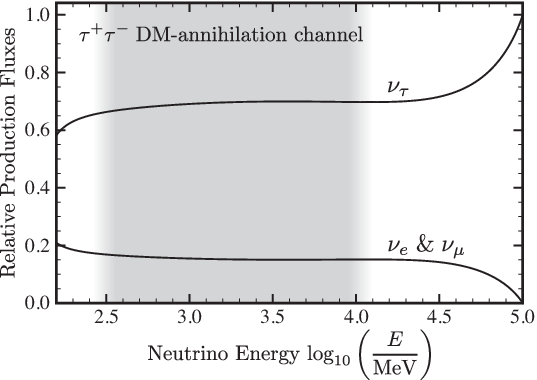
The second potential source of energy dependence, the matrix $\underline{U\hskip-2.56073pt}\hskip 2.56073pt_{\hskip-0.85358ptm}$, can also be tamed: for neutrino energies sufficiently above the 2nd resonance, $\underline{U\hskip-2.56073pt}\hskip 2.56073pt_{\hskip-0.85358ptm}$ approaches an $E$-independent constant matrix (see e.g., Ref. [1]). For this reason, we will consider only energies well above $E_{R}^{h}\sim 0.3\,$GeV, so that $\underline{U\hskip-2.56073pt}\hskip 2.56073pt_{\hskip-0.85358ptm}$ is effectively constant.

Some energy dependence will also be introduced in the flavor ratios by the adiabatic-to-nonadiabatic transition of the 1st resonance. This occurs at energies at and above $E_{N\!A}^{l}\sim 10\,$GeV [1]. As can be seen in Figs. 3 and 4 of Ref. [1], the effects of the 1st resonance are mild; to ignore these effects would introduce little uncertainty into our calculation, and the effects could be included in a more complete analysis. However, we will simply restrict our study to energies below $E_{N\!A}^{l}$ to shield our analysis from “contamination” due to the 1st resonance. Thus, we arrive at, and define, a “sweet region” in energy for our analysis:

The results presented below will hold within this special region of energy.

The remaining and most important source of structure in the flavor spectra arises from the neutrino level-crossing probabilities at the resonances, which are described by the jump matrix $\underline{P\hskip-1.99168pt}\hskip 1.99168pt$. The transition from the adiabatic (i.e., no level-crossing) to the nonadiabatic (i.e., complete level-crossing) regime at high energies can leave a dramatic imprint in the terrestrial flavor-flux ratios.

In Ref. [1], the energy $E_{N\!A}^{h}$ characterizing the onset of this adiabatic-to-nonadiabatic transition was defined implicitly by setting $P_{c}^{h}(E_{N\!A}^{h})$ in the crossing-probability matrix to $e^{-3}\simeq 5\%$. Numerically, this onset energy is $E_{N\!A}^{h}\simeq 750\,\sin^{2}\theta_{13}\,$GeV. (An expression for the crossing probability is given below in Eq. (13).) The 2nd resonance occurs in the neutrino sector for the normal hierarchy with $\delta m^{2}_{32}>0$, and in the antineutrino sector for the inverted hierarchy with $\delta m^{2}_{32}<0$.

The above discussion shows that we may identify any observable energy dependence of the flavor spectra in the sweet region as due to the adiabatic-to-nonadiabatic transition at $E_{N\!A}^{h}$. In turn, the energy dependence in this sweet region will implicate the value of a small but nonzero $\theta_{13}$ as well as the neutrino mass hierarchy. In particular, at small $\theta_{13}$ the nonadiabatic jump probability is $\exp(-\Gamma\,\theta_{13}^{2})$. The “adiabaticity parameter” $\Gamma$ can be written in terms of the length scale $\lambda_{\odot}=|\frac{d}{dr}\ln N_{e}|^{-1}$ for the change in the electron density $N_{e}$ at the resonance region (corresponding to one $e$-folding in density for an exponential profile like that of the Sun), and the neutrino oscillation length in vacuum $\lambda_{v}=4\pi\,E/\delta m^{2}$ as $\Gamma=4\pi^{2}\,\lambda_{\odot}/\lambda_{v}$. The important feature for our purposes is that $\Gamma$ scales as $1/E$ and is therefore large, roughly $300$–$10\,000$, across the low energies of our sweet region. It is this large size of $\Gamma$ that produces an observable signal even for extremely small $\theta_{13}$. Qualitatively, we expect sensitivity to $\theta_{13}$ in the sweet region for $\theta_{13}$ as small as $1/\sqrt{\Gamma}\gtrsim 10^{-2}\sim 0.5^{\circ}$. In Sec. IV, we show quantitatively that this is indeed the case.

There is also a terrestrial source of energy dependence in the flavor ratios. This arises from matter effects for neutrinos and antineutrinos traversing the Earth. The effect has been well worked out in publications [16]; it is somewhat complicated (best addressed with a numerical code), and we will not include it in this paper. We do give here some general remarks [1] about the Earth matter effect that are relevant for our present purposes. The resonant energies in Earth related to the solar scale $\delta m^{2}_{21}$ are below the sweet region (at $\sim 25\,$MeV and $\sim 100\,$MeV for the Earth’s core and mantle, respectively), while the resonant energies in Earth related to the atmospheric-scale $\delta m^{2}_{32}$ fall right in the sweet region, at $\sim 2\,$GeV and $\sim 10\,$GeV for the Earth’s core and mantle, respectively. As with the solar resonance, for a normal mass hierarchy the relevant resonance in Earth occurs in the neutrino but not the antineutrino sector. And again as with the solar resonance, for an inverted mass hierarchy the relevant resonance in Earth occurs in the antineutrino but not the neutrino sector. The resonant amplification can be quite large, but the effect can be mitigated by a resonant oscillation wavelength scaling like $1/\theta_{13}$. The requirement that at least a quarter of the oscillation length must lie within the Earth to “feel” the matter effects leads to a nadir-dependent condition on $\theta_{13}$. For a neutrino with zero nadir angle, $\theta_{13}\gtrsim 0.5^{\circ}(E/{\rm GeV})$ is required to feel the matter; for other nadir angles, larger values of $\theta_{13}$ are required to feel the matter. In a more complete analysis involving real data, terrestrial-matter effects should then no longer be ignored.

It is worth remarking here what would change if the WIMP mass were, say, a TeV rather than the $100\,$GeV we have assumed [13]. Surely, the available phase space for the produced neutrinos is increased. Moreover, in Ref. [12] it is shown that the upper end of the neutrino energy spectrum scales linearly with the WIMP mass, tending to enlarge the energy region in which the flavor ratios are constant. However, the sweet region remains between $0.3$ and $10\,$GeV because it is determined solely by the effects of solar matter on neutrino propagation. It follows that the phase space of the sweet region relative to the enlarged total phase space now represents a smaller fraction, so that less sweet-region neutrinos are available. More importantly, according to Eq. (3) the expected neutrino flux from WIMP annihilation in the Sun scales as $M_{\rm WIMP}^{-2}$, and so would be down by an additional factor of 100 for annihilation of TeV WIMPs compared to $100\,$GeV WIMPs.

One must inevitably ask what event rate at Earth might be expected from solar WIMP annihilation to (anti)neutrinos in the sweet region, and what rate is needed to observe structure in the terrestrial flavor spectra. We attend to first of these questions in the next section, and discuss the requirement for statistical significance in our final Sec. VI.

Theory suggests that the age of the Sun exceeds the equilibration time between solar capture of WIMPs and their subsequent annihilation in the Sun [17]. Consequently, the WIMP annihilation rate is given by half of the WIMP capture rate, where the “half” just reflects the fact that it takes two captures to enable one two-body annihilation. The WIMP capture rate by the Sun is given in Ref. [17]:

where

is a fiducial factor. Here, $\sigma_{\rm WIMP}$ and $M_{\rm WIMP}$ are the unknown WIMP–nucleon scattering cross section and mass, while $\rho_{\rm WIMP}$ and $v_{\rm WIMP}$ denote the density and rms velocity of the local WIMP population. Each parenthetical fraction displays typical values, except that the fiducial value shown for $\sigma_{\rm WIMP}$ is the present upper limit for the spin-dependent cross section [18, 19]; it must therefore be viewed as optimistic. The inverse quadratic dependence of the rate on the WIMP mass is easily understood: one factor arise from the conversion of WIMP mass density $\rho_{\rm WIMP}$ to number density, and the other factor is kinematic, reducing the capture efficiency when the beam and target masses are mismatched. The fiducial values for today’s local WIMP density and rms velocity serve as numerical guidelines, but in fact the integrated history of WIMP capture by the Sun over large look-back times may yield values that do not adhere to these guidelines.

The WIMP–nucleon cross section in Eq. (4) above is the sum of a spin-independent cross section and a spin-dependent cross section, each averaged over the target matter in the Sun’s core. Experiments on Earth that search directly for WIMPs typically use target materials with large nucleon number, and so are better suited to limit (or detect) the spin-independent cross section [20]. Direct-search limits on the spin-dependent cross section are five orders of magnitude weaker than the limits on the spin-independent cross section. Since the solar material is mainly hydrogen, solar capture of WIMPs is very sensitive to the spin-dependent cross section.

An experimental measurement of the solar neutrino flux from WIMP annihilation would bypass the theoretical uncertainties just listed. So far, experiments have yielded only upper limits on this flux inferred from final-state muons with energies above a GeV [18, 19]. It is interesting to note that the bounds on the spin-dependent WIMP cross section inferred from these experimental neutrino-flux constraints are stronger than the bounds coming from direct searches for WIMPs [21].

We continue by considering the mean multiplicity of neutrinos, $\xi_{\nu}$, produced per annihilating WIMP (not WIMP pair), a quantity we anticipate to be of order unity. We can then estimate the total neutrino flux at Earth [22]:

The background from “atmospheric neutrinos,” i.e., the neutrinos resulting from the decay of charged pions produced by cosmic-ray interactions in our atmosphere, has been calculated by many groups with convergent results. A typical energy spectrum in the GeV region can be found in Ref. [7]. It approximately obeys $1.2\times 10^{6}\,\left(\frac{E}{\rm GeV}\right)^{-2.75}({\rm GeV\cdot yr\cdot cm^{2}})^{-1}$ for $({\nu_{\mu}}+{\bar{\nu}}_{\mu})$; the all-flavor flux would be about three times larger. The integrated all-flavor flux above a GeV is then about $2\times 10^{6}/{\rm yr\ cm^{2}}$, with the spectral-index factor nearly compensating the flavor factor. This background flux is roughly twenty times the maximally allowed solar WIMP neutrino flux. Moreover, the background flux has a flavor content that varies with direction on the sky. The down-coming atmospheric neutrinos will show the $1:2$ ${\nu_{e}}$ to ${\nu_{\mu}}$ flavor ratio characteristic of the complete pion decay chain, as the muon decay length at lower energies is shorter than its atmospheric height, and the neutrino pathlength is shorter than its vacuum oscillation length $L_{\rm osc}=4\pi\,E/\delta m^{2}\sim 1000\,(E/{\rm GeV})\,$km. In contrast, the upcoming neutrinos will show a 1:1 flavor ratio, since half of the ${\nu_{\mu}}$’s will have oscillated into ${\nu_{\tau}}$’s. On the bright side, the solar fraction of solid angle on the sky is quite small, approximately $[\pi\,(R_{\odot}/{\rm AU})^{2}]/4\pi\sim 5.4\times 10^{-6}$. So one may hope that a cut favoring the direction to the Sun would greatly increase the signal-to-background ratio. However, the mean scattering angle for neutrinos below $10\,$GeV is large, $\theta_{\rm scatt}\sim 20^{\circ}\sqrt{10\,{\rm GeV}/E}$. The 24-hour angular modulation expected in the solar signal will help reduce the unmodulated atmospheric background. In addition, there has been some recent discussion of possible very large detectors [23], and some development in directional reconstruction of neutrinos at lower energies [24, 25]. There have also been recent studies of using event topologies to achieve partial “statistical” separation of neutrino and antineutrino data samples [26].

Multiplying the solar WIMP neutrino flux by (i) the neutrino–nucleon cross section, by (ii) the target number of nucleons given by

and by (iii) the fraction of incident neutrino flux in the sweet region $\Delta E(\textrm{SR})$ from 0.3 to $10\,$GeV

one obtains the event rate within the sweet energy region. For a $100\,$GeV WIMP mass, inspection of the theoretical neutrino spectra in Ref. [12] suggests a value $\sim 20\%$ for $f_{\nu}$, the fraction of neutrino flux in the sweet region between 0.3 and $10\,$GeV. As a fiducial event rate, we therefore take

For some perspective on the 140 events per year, we may ask how many events per year are to be expected in a proton-decay experiment at a megaton detector. The present limits on the lifetime of protons to decay to various modes are typically $10^{35}\,$yr. The nucleon number in a megaton is $10^{12}\,N_{A}=6\times 10^{35}$. So the expected event rate is

We see that the rates for detection of solar neutrinos in the sweet region from WIMP annihilation and for detection for proton decay are comparable (although the backgrounds are different).

To proceed, we need explicit expressions for the neutrino flavor spectrum produced by WIMP annihilation in the Sun’s core in the range $0.3$–$10\,$GeV. We begin by parameterizing the relative production fluxes $w_{\alpha}$. In many models, the dominant WIMP-annihilation channels are $b\,\overline{b}$, $\tau^{+}\tau^{-}$, and $W^{+}W^{-}$. The neutrino spectrum from each channel has been calculated (see, e.g., Ref. [12]), but the branching ratios to these channels depend on the specific model. Fortunately, WIMP decay obeys $w_{e}(E)=w_{\mu}(E)$ to a very good approximation [12]. Since the normalization $w_{e}+w_{\mu}+w_{\tau}=1$ holds at any energy, the parametrization of the relative flavor spectra at production requires just one WIMP-model-dependent function $f_{F}(E)$.

We define $f_{F}$ operationally via $w_{e}=w_{\mu}=\frac{1}{3}-f_{F}$ and $w_{\tau}=\frac{1}{3}+2\,f_{F}$. Positivity of the $w_{\alpha}$ then implies the bound $-\frac{1}{6}\leq f_{F}\leq+\frac{1}{3}$. As defined, $f_{F}$ is the deficit of $w_{e}$ or $w_{\mu}$ from $\frac{1}{3}$ at injection in the solar core. Since maximal mixing effects symmetrization of ${\nu_{\mu}}$ and ${\nu_{\tau}}$, it is also useful to view $f_{F}$ as the excess of $w_{\not\hskip 0.56905pte}\equiv w_{\mu}+w_{\tau}$ from $\frac{2}{3}$. To order $f_{F}^{2}$, the ratios ($w_{e}/w_{\tau}$) and ($w_{\mu}/w_{\tau}$) at injection are $1-9\,f_{F}+36\,f_{F}^{2}$.

For comparative purposes later, it is also useful interpret $f_{F}$ in terms of the evolved flavor probabilities $W_{\alpha}$ in the absence of matter effects. The flavor density matrix at injection, in the flavor basis, is given by

Using the tribimaximal mixing values to write this in the mass basis, and invoking phase averaging to remove the off-diagonal elements, one is left with just

Then, the relative flavor probabilities $W_{\alpha}$ are just $\langle\,\nu_{\alpha}\,|\,\rho_{F}\,|\,\nu_{\alpha}\rangle$. The results for vacuum transitions are $W_{e}={\overline{W}}_{e}=\frac{1}{3}-\frac{1}{3}\,f_{F}$, and $W_{\mu}=W_{\tau}={\overline{W}}_{\mu}={\overline{W}}_{\tau}=\frac{1}{3}+\frac{1}{6}\,f_{F}$. The vacuum value for the ratios $W_{\mu}/W_{e}$ and ${\overline{W}}_{\mu}/{\overline{W}}_{e}$ to order $f_{F}^{2}$ are $1+\frac{3}{2}\,f_{F}+f_{F}^{2}$.

Although actual WIMP properties are unknown, we may consider two of the aforementioned annihilation channels, $b\,\overline{b}$ and $\tau^{+}\tau^{-}$, as generic examples. We have argued that in our sweet region, the function $f_{F}(E)$ is reduced to an energy-independent number $f_{F}$ for the $\tau^{+}\tau^{-}$ and $b\,\bar{b}$ annihilation modes of the solar WIMPs. Our fitted values for $f_{F}$ in these channels are $-0.09\pm 0.01$ and $+0.182\pm 0.001$, respectively.

It is worth mentioning that in some WIMP models the annihilation to fermions proceeds through Higgs-like couplings. We then expect the $b\,\bar{b}$ mode to dominate, but also a branching fraction to $\tau^{+}\tau^{-}$ given by $(m_{\tau}/m_{b})^{2}/3\sim 5\%$, where the $\frac{1}{3}$ reflects the $b\,\bar{b}$ mode’s color factor. In the sweet region, the $f_{F}$’s for the $b\,\bar{b}$ and $\tau^{+}\tau^{-}$ modes have opposite signs, so the average $f_{F}$ for the fermionic channel is smaller in magnitude than $f_{F}(b\,\bar{b})$ and $f_{F}(\tau^{+}\tau^{-})$. However, the $b\,\bar{b}$ mode, and thus its concomitant $f_{F}$ value, dominate: an estimate employing the injection spectra given in Ref. [12] indeed yields $f_{F}(\rm Higgs)\simeq-0.07\pm 0.01$ in proximity to the $-0.09$ value for $b\,\bar{b}$ mode. We remark that the neutrino spectrum from the $\tau^{+}\tau^{-}$ mode is harder than that from the $b\,\bar{b}$ mode, and at energies above the sweet region, of no relevance to the present paper, the $\tau^{+}\tau^{-}$ mode becomes increasingly important and eventually comes to dominate. For the $W^{+}W^{-}$ mode, $f_{F}$ behaves quite differently: it rises nearly linearly with energy in the sweet region: $f_{F}(W^{+}W^{-})=-0.029+0.014\,(E/\textrm{GeV})$. The values for the various $f_{F}$’s presented in this paragraph have been estimated using the results in Ref. [12]; they are also collected in Table 1.

We note that for equal initial flavors ($f_{F}$=0), the resulting terrestrial flavor ratios are also democratic [1], i.e., $W_{e}=W_{\mu}=W_{\tau}=1/3$. This is most easily seen by noting that the commutator in the density-matrix evolution equation $i\,\frac{d\rho}{dt}=[H,\,\rho]$ vanishes for $\rho$ proportional to the identity matrix regardless of whether $H$ is the vacuum or matter Hamiltonian. Thus, it is only the order 7–18% $f_{F}$-value differences in the initial flavor spectrum that evolve nontrivially. If flavor differences were not amplified by intervening matter effects, an event sample of about $(n/15\%)^{2}$ would be necessary to yield an $n$-sigma statistical inference of this difference. However, we will see shortly that matter effects, quadratically sensitive to $\theta_{13}$ and to the neutrino mass hierarchy, may amplify the flavor difference considerably.

For further progress, we also need explicit expressions for $\underline{U\hskip-2.56073pt}\hskip 2.56073pt$, $\underline{P\hskip-1.99168pt}\hskip 1.99168pt$, and $\underline{U\hskip-2.56073pt}\hskip 2.56073pt_{\hskip-0.85358ptm}$ appearing in Eq. (1). In the sweet region, the level-crossing probability at the lower resonance is zero, as explained above. The fact that Eq. (1) is linear in the level-crossing probability matrix $\underline{P\hskip-1.99168pt}\hskip 1.99168pt$ allows one to write a simple equation for the flavor evolution,

valid in the sweet region. The pre-factor of $\frac{1}{4}$ in front of the square brackets is chosen for convenience. The flavor-indexed quantities $A_{\alpha}$ and $B_{\alpha}$, $\alpha=e,\mu,\tau$, are determined by the neutrino mixing parameters at the Sun’s core (where $\nu_{e}\sim\nu_{3}$) and at Earth (vacuum values) [27]. Since the mixing parameters are energy independent in the sweet region, so too are $A_{\alpha}$ and $B_{\alpha}$. The flavor-vectors $B_{\alpha}$ and $A_{\alpha}$ do depend on the neutrino mass hierarchy and on incident neutrino versus antineutrino. Importantly, the entire energy dependence in the evolution equation (12) is contained in the level-crossing probability $P_{c}^{h}(E)$ at the 2nd resonance, given by the expression

In this expression, $\Theta$ denotes the unit-step function, and ${\cal O}(\delta m^{2}_{21}/|\delta m^{2}_{32}|)\sim 0.03$ terms have been dropped. As mentioned in the overview section, the adiabaticity parameter $\Gamma$ may be written as

where

is the scale of density change (the distance for an $e$-folding change in the solar density, equal to $6.6\times 10^{4}\,$km) and $\lambda_{v}\equiv 4\,\pi\,E/\delta m^{2}_{32}$ is the oscillation length in vacuum. Consequently, $\Gamma$ scales as $1/E$, and we define a constant ${\tilde{\Gamma}}$ via

where

for the higher-energy resonance in solar matter. With Eqs. (14)–(17) at hand, it is apparent that $\Gamma\mathrel{\vbox{\hbox{$>$}\hbox{$\sim$}}}300$. This large $\Gamma$ value, together with the experimental input $\sin^{2}\theta_{13}\ll 1$ and the fact that $E>E^{h}_{R}$ in the sweet region, has been used to obtain the second line of Eq. (13).

Note that the only neutrino mixing parameter contained in $P_{c}^{h}(E)$ is $\theta_{13}$, and it enters essentially squared in an exponent. It follows then, that the dominant energy dependence of the terrestrial flavor ratios in the sweet region is governed by $\theta_{13}$, as advertised in the introduction. Moreover, the sensitivity of flavor evolution through the adiabatic-to-nonadiabatic transition is exponentially sensitive to $\theta_{13}^{2}$.

From Eqs. (13) and (16), we infer the onset energy for $E_{N\!A}^{h}$ for the adiabatic-to-nonadiabatic transition to be

Neutrinos with energy $E_{R}^{h}<E\lesssim E_{N\!A}^{h}$ will experience adiabatic level-repulsion at the 2nd resonance, whereas neutrinos with $E\gg E_{N\!A}^{h}$ will experience nonadiabatic level-crossing at the 2nd resonance. We remark that although it is true in the Sun that the adiabatic-to-nonadiabatic transition energy $E_{N\!A}^{h}$ exceeds the resonant energy $E_{R}^{h}$, this ordering is not in in general guaranteed. The ratio of the two energies is

Numerically, the term in brackets is 1800 for the Sun. It is this fortuitously large value for the Sun that allows the adiabatic-to-nonadiabatic transition to probe $\theta_{13}$ values all the way down to $\theta_{13}\sim(\frac{2\pi}{3}1800)^{-\frac{1}{2}}\sim 1^{\circ}$.

We proceed by defining the energy $E_{1/2}$ at which the crossing probability is one half. From Eqs. (13) and (16) we readily find that

Let us also define the width of the change in crossing probability as $\Delta E=E_{+}-E_{-}$, where $P^{h}_{c}(E_{-})=1/e$ and $P^{h}_{c}(E_{+})=1-1/e$. This yields

It is seen that $E_{1/2}$ as well as $\Delta E$ are approximately equal to $4\,\sin^{2}\theta_{13}\approx 4\,\theta^{2}_{13}$ in units of TeV. Both $E_{1/2}$ and $\Delta E$ are very sensitive probes of the unknown $\theta_{13}$. The experimental upper bound $\sin\theta_{13}\leq 0.22$ at $3\sigma$ establishes that $\theta_{13}\simeq\sin\theta_{13}$ to better than 1% accuracy. Accordingly, we may invert Eq. (20) to obtain

For $\theta_{13}$ in the phenomenologically interesting range $0.6^{\circ}\leq\theta_{13}\leq 3^{\circ}$, Eq. (20) tells us that $E_{1/2}$ lies within the sweet region. Then, the inverse Eq. (22) establishes that a measurement of the adiabatic-to-nonadiabatic transition energy, via changing flavor ratios, probes the $\theta_{13}$ mixing angle in this very interesting range from $0.6^{\circ}$ to $3^{\circ}$. Equation (22) is the most important result of this paper. We show below that the flavor signal is also sensitive to the neutrino mass hierarchy.

The ratio $\Delta E/E_{1/2}\simeq 1.19$ is independent of $\theta_{13}$. Consequently, the number of events needed to establish $E_{1/2}$, and thereby $\theta_{13}$, is independent of $\theta_{13}$ or $E_{1/2}$. Of course, the necessary event number will depend on the magnitude of flavor change over the transition region. Since $\Delta E\sim E_{1/2}$, we have that $\Delta E/E=\Delta\ln E\sim 1$. From this we infer that the relevant event sample must span about a natural log in energy about $E_{1/2}$ to map out the transition region in detail, again independent of $\theta_{13}$ or $E_{1/2}$. However, to measure the gross change in flavor ratios across the transition, an event sample may be drawn from an energy region as large as the entire sweet region, 0.3 to $10\,$GeV. The availability of this wide energy range for the data sample is fortunate, for at the relatively low energies of the sweet region, large uncertainties are expected in the reconstruction of the neutrino energy from the measured charged lepton.

The change in the flavor ratios across the adiabatic-to-nonadiabatic transition region of width $\Delta E$ centered on $E_{1/2}$ is the signal. The magnitude of the flavor change across the transition region is determined by Eq. (12) and depends on the parameters $A_{\alpha}$ and $B_{\alpha}$. These parameters in turn depend on the neutrino mixing angles, the mass hierarchy, and the particle type (neutrinos vs. antineutrinos). The two hierarchies and the neutrino versus antineutrino type lead to four possibilities. To distinguish among these possibilities, we employ the notation $A_{\alpha}^{\rm NH}$, $\overline{A}{}_{\alpha}^{\rm IH}$, etc., where the bar denotes the antineutrino case and the superscripts NH and IH refer to the normal and inverted hierarchy, respectively. For our present purposes, it is sufficient to employ the “tribimaximal” values [28] for the two large mixing angles, i.e., to set $\sin^{2}\theta_{23}^{\rm TBM}=1/2$ and $\sin^{2}\theta_{12}^{\rm TBM}=1/3$. The phenomenological accuracy of this approximation is very good, as is summarized in Ref. [29].

Although we employ the tribimaximal values for $\theta_{32}$ and $\theta_{12}$ in what follows, we nevertheless exhibit in Table 2, for possible future use, the first-order corrections to the $A_{\alpha}$ and $B_{\alpha}$ that result if the neutrino mixing angles deviate from their tribimaximal values. To this end, we have denoted the deviations from the tribimaximal case by $\delta\theta_{jk}\equiv\theta_{jk}-\theta_{jk}^{\rm TBM}$. The expressions in Table 2 result from a calculation paralleling that in Appendix D of Ref. [1]. The $3\sigma$ experimental uncertainties in the angles are [30]

Consequently, future data may mandate deviations from the tribimaximal-based $A_{\alpha}$ and $B_{\alpha}$ used in this work.

In the first subsection, we present results valid to all orders in $f_{F}$. In particular, we provide figures for the $\tau^{+}\tau^{-}$ annihilation mode generated with the complete energy dependence of $f_{F}(E)$ over an energy range that includes the sweet region. In the second subsection, we present analytic formulas for the sweet region valid to order $f_{F}^{2}$ and compare (favorably) their validity with the more exact figures.