How close can an Inhomogeneous Universe mimic the Concordance Model?

Peter Dunsby^⋄,†,⋆, Naureen Goheer^†, Bob Osano^†, Jean-Philippe Uzan^†,‡ Affiliation:

\diamond

Centre for Astrophysics, Cosmology and Gravitation, University of Cape Town, Rondebosch, 7701, South Africa Affiliation:

{\dagger}

Department of Mathematics and Applied Mathematics, University of Cape Town, Rondebosch, 7701, South Africa Affiliation:

\star

South African Astronomical Observatory, Observatory, Cape Town, South Africa Affiliation:

{\ddagger}

Institut d’Astrophysique de Paris, UMR-7095 du CNRS, Université Paris-VI Pierre et Marie Curie, 98bis bd Arago, F-75014 Paris (France)

August 24, 2026

Abstract

Recently, spatially inhomogeneous cosmological models have been proposed as an alternative to the $\Lambda$ CDM model, with the aim of reproducing the late time dynamics of the Universe without introducing a cosmological constant or dark energy. This paper investigates the possibility of distinguishing such models from the standard $\Lambda$ CDM using background or large scale structure data. It also illustrates and emphasizes the necessity of testing the Copernican principle in order to confront the tests of general relativity with the large scale structure.

pacs

98.80.Cq

I Introduction

The analysis of all existing astrophysical data sets, including the observation of the cosmic microwave background [1], type Ia supernovae (SNIa) luminosity distance measurements [2] and the large scale structure [3, 4, 5]) leads to the conclusion that our cosmological model requires the introduction of a cosmological constant, representing 72% of the total matter content of the Universe today, together with a Cold Dark Matter component which significantly dominates ordinary baryonic matter. Although such a model remains the best fit to all available cosmological data, understanding the physical origin of the late time acceleration of the cosmic expansion motivates many investigations on the basis of our cosmological model [6, 7].

As long as the Copernican principle is assumed to hold, there are two possibilities which could explain these observations. Either one introduces a dark energy component (the cosmological constant being the simplest possibility) or one allows for a modification of General Relativity on astrophysical large scales (see e.g. Ref. [8] for a recent review and Ref. [9] for recent reviews on the large variety of dark energy models).

The standard concordance model of the universe lies heavily on the assumption that the universe is spatially isotropic and homogeneous on large scales and can thus be described by a Friedmann-Lemaître (FL) spacetime. Since this principle stands at the heart of our interpretation of all cosmological observations, it is important to ensure that it holds with a sufficient accuracy on the scales on which we perform our observations. Recently, various tests of the Copernican principle have been proposed [10, 11, 12, 13]. It was also shown that the need for dark energy can be suppressed if our universe is inhomogeneous on scales of some fraction of the Hubble radius [14, 15, 16, 17, 19], the underlying reason being that we actually have access to data only on our past null cone so that it is possible to design spacetime geometries that will enjoy the same (low redshift) past-light cone structure as the one of a FL model without introducing a cosmological constant [14, 15, 16, 17] (see however Ref. [18] for some limitations).

In any FL model, the complete dynamics of this universe is encoded in a single function of time, the scale factor $a(t)$ . This implies that all the background observations, e.g., luminosity distance-redshift relation, angular distance, look-back time, etc.., are functionals of the Hubble rate $H(z)$ . More importantly, in a $\Lambda$ CDM model, the late time growth of density perturbation on sub-Hubble scales is also a function of $H(z)$ , provided we restrict ourselves to linear evolution. This implies that there exist rigidities between different set of independent observables ( from the background and at the level of perturbation theory) that can be used to test the underlying hypothesis of the model [6, 7, 8].

The goal of this article is to investigate how two models that reproduce the same background data on the past-light cone can be distinguished. In Section II, we recall the main properties of the background spacetime and we emphasize that the time drift of the cosmological redshift is not only in principle but also in practice a good test of the Copernican principle. Section III describes the perturbation theory and discusses various approximations. In Section IV, we describe the integration of this simplified model in order to obtain the transfer functions on the past light-cone. This exercise allows us to describe the way one distinguishes a LTB model from a Friedmann model that share the same light-cone background structure. It also clearly illustrates one of the important limitations of most of the tests of general relativity on astrophysical scales since they encode the Copernican principle in their construction.

II Background spacetime dynamics

II.1 Description of the geometry

We consider a spatially spherically symmetric and inhomogeneous universe described by a Lemaître-Tolman-Bondi (LTB) the metric [20]:

{\rm d}s^{2}=-{\rm d}t^{2}+\frac{X^{2}(r,t)}{1+2E(r)}{{\rm d}r^{2}}+R^{2}(r,t){\rm d}\Omega^{2}\,,

(1)

with $X=R^{\prime}$ , using the convention $R^{\prime}=\partial_{r}R$ and $\dot{R}=\partial_{t}R$ . It is convenient to define

2E(r)\equiv-k(r)r^{2},

(2)

as well as the two Hubble expansion rates

H_{\perp}\equiv\frac{\dot{R}}{R},\qquad H_{\parallel}\equiv\frac{\dot{X}}{X}=\frac{\dot{R}^{\prime}}{R^{\prime}}\,.

(3)

The field equations for such a spacetime are given by

\frac{\dot{R}^{2}}{R^{2}}=\frac{M(r)}{R^{3}}+\frac{2E(r)}{R^{2}},\qquad 8\pi G\rho(r,t)=\frac{M^{\prime}}{R^{2}R^{\prime}},

(4)

from which it can be checked that the continuity equation

\dot{\rho}+(2H_{\perp}+H_{\parallel})\rho=0

(5)

is satisfied. These equations can be solved parametrically as

R(t,r)=\frac{m(r)r}{2\hat{k}(r)}\phi^{\prime}(\eta)\,,\quad t-t_{B}(r)=\frac{m(r)}{2\hat{k}^{3/2}(r)}\phi(\eta)\,,

(6)

where we have defined $\phi(\eta)=(\eta-\sin\eta,\eta^{3}/6,\sinh\eta-\eta)$ and $\hat{k}=(k,r^{-2},-k)$ respectively for $k$ positive, null and negative and defined $m(r)=M(r)/r^{3}$ . This solution involves three arbitrary functions $M(r)$ , $t_{B}(r)$ and $k(r)$ (or equivalently $E(r)$ ) but only two of them are actually needed since one can fix one of them by a proper choice of the radial coordinate $r$ .

To finish this description of the background spacetime, let us compute the expressions of $\dot{R}$ , $R^{\prime}$ and $\dot{R}^{\prime}$ that we will need later on. It is obvious from Eq. (4) that

\dot{R}=\sqrt{\frac{M(r)}{R}+2E(r)}.

(7)

Then, from Eq. (6) we deduce that

R^{\prime}=\left(\frac{M^{\prime}}{M}-\frac{E^{\prime}}{E}\right)R-\left[t_{B}^{\prime}-\left(\frac{3}{2}\frac{E^{\prime}}{E}-\frac{M^{\prime}}{M}\right)(t-t_{B})\right)\dot{R},

(8)

and then that

$\displaystyle\dot{R}^{\prime}$	$\displaystyle=$	$\displaystyle\frac{1}{2}\frac{E^{\prime}}{E}\dot{R}$	(9)
		$\displaystyle+\left[t^{\prime}_{B}-\left(\frac{3}{2}\frac{E^{\prime}}{E}-\frac{M^{\prime}}{M}\right)(t-t_{B})\right]\frac{M}{2R^{2}},$	(9)
	$\displaystyle=$	$\displaystyle\frac{1}{2\dot{R}}\left(\frac{M^{\prime}}{R}-\frac{MR^{\prime}}{R^{2}}+2E^{\prime}\right).$	(10)

The case of a spatially homogeneous universe is recovered in the case where $t_{B}(r)=0$ , $m=$ constant and $k=$ constant. It follows that $R(r,t)=a(t)r$ and $X(r,t)=a(t)$ where $a$ is the scale factor. The spacetime metric thus takes a FL form

{\rm d}s^{2}=-{\rm d}t^{2}+a^{2}(t)\left[{\rm d}\chi^{2}+f^{2}_{K}(\chi){\rm d}\Omega^{2}\right],

(11)

with $f_{K}(\chi)=(\sin\chi,\chi,\sinh\chi)$ depending on the sign of $K$ .

II.2 Light cone equation

Most of our analysis focuses on what is actually observed on our past light-cone, which can be defined by solving the null geodesic equation. Given a null geodesic with tangent vector $k^{\mu}$ , the redshift of any object is defined by

1+z\equiv\frac{(k_{\mu}u^{\mu})_{em}}{(k_{\mu}u^{\mu})_{rec}}\,,

(12)

where $u^{\mu}$ is the tangent vector to the matter worldlines. It follows that the geodesic equation $k^{\mu}\nabla_{\mu}k^{\nu}=0$ for a null-vector reduces to

	$\displaystyle\frac{{\rm d}t}{{\rm d}z}$	$\displaystyle=$	$\displaystyle-\frac{1}{(1+z)H_{\parallel}},$		(13)
	$\displaystyle\frac{{\rm d}r}{{\rm d}z}$	$\displaystyle=$	$\displaystyle\frac{\sqrt{1+2E(r)}}{(1+z)\dot{R}^{\prime}}.$		(14)

This defines our past lightcone that we shall denote by

{\mathcal{C}}_{-}:\,\,\{r=r_{*}(z),t=t_{*}(z),\quad r_{*}(0)=0,t_{*}(0)=t_{0}\}.

The redshift is the observational radial coordinate which can be expressed as a look-back time or distance, assuming a cosmological model [21]. One can indeed use either $r$ , $t$ or $z$ as integration variable, the important point being that only 2 of the three quantities $(t_{*},r_{*},z)$ are independent.

When evaluated along the past light-cone, the function $R(r,t)$ is related to the angular distance $D_{A}$ by

{\cal R}_{0}(z)\equiv R[t_{*}(z),r_{*}(z)]=D_{A}(z)\,.

(15)

This observational relation can be used to set one constraints on the two arbitrary functions of the LTB spacetime. It is useful to redefine the functions introduced previously when evaluated on the past-light cone as

{\cal R}_{10}\equiv\dot{R}[t_{*},r_{*}],\quad{\cal R}_{01}\equiv R^{\prime}[t_{*},r_{*}],

(16)

and

{\cal R}_{11}\equiv\dot{R}^{\prime}[t_{*},r_{*}],

(17)

to be considered either as functions of $z$ or $r_{*}$

We choose $r_{*}$ as the radial distance along the light cone and fix it by imposing

\frac{{\cal R}_{01}}{\sqrt{1+2E}}=1,

(18)

which simplifies the past light-cone equation reducing it to

\displaystyle\frac{{\rm d}t_{*}}{{\rm d}r_{*}}=-1,\qquad\frac{{\rm d}z}{{\rm d}r_{*}}=\frac{(1+z){\cal R}_{11}(r_{*})}{\sqrt{1+2E(r_{*})}}.

(19)

II.3 Reconstruction procedure of a LTB geometry

II.3.1 General procedure

With the choice of coordinates (18) the derivative of ${\cal R}$ along the past light-cone is given by

\displaystyle\frac{{\rm d}{\cal R}}{{\rm d}r_{*}}

\displaystyle=

\displaystyle{\cal R}_{01}-{\cal R}_{10}

(20)

and Eqs. (8-9) can be rewritten as

	$\displaystyle\left[{\cal R}_{0}-(t-t_{B}){\cal R}_{10}\right]\frac{M^{\prime}}{M}+\left[\frac{3}{2}(t-t_{B}){\cal R}_{10}-{\cal R}_{0}\right]\frac{E^{\prime}}{E}$
	$\displaystyle\qquad\qquad\qquad-{\cal R}_{10}t^{\prime}_{B}={\cal R}_{01}=\sqrt{1+2E},$		(21)
	$\displaystyle\frac{M}{2{\cal R}^{2}_{0}}\frac{M^{\prime}}{M}(t-t_{B})+\left[\frac{1}{2}{\cal R}_{10}-\frac{3}{2}(t-t_{B})\frac{M}{2{\cal R}_{0}^{2}}\right]\frac{E^{\prime}}{E}$
	$\displaystyle\qquad+\frac{M}{2{\cal R}^{2}_{0}}t^{\prime}_{B}={\cal R}_{11}.$		(22)

Hence, provided $D_{A}(z)$ is known from observation, we fix ${\cal R}_{0}$ and then Eqs. (19-22) give 4 equations for the 6 unknown functions $(t,z,M,E,t_{B},{\cal R})$ of $r_{*}$ . One thus need to fix 2 conditions to completely specify the model.

This approach was investigated in Ref. [16] who designed various LTB solution sharing the same $D_{A}(z)$ relation as a FL spacetime by imposing either $t_{B}=0$ or $k=$ constant. We follow the same line and consider LTB models that reproduce the angular distance-redshift relation of a fiducial standard flat $\Lambda$ CDM model. For such a FL universe

\frac{H_{FL}^{2}}{H^{2}_{0}}=\Omega_{{\rm m}0}(1+z)^{3}+\Omega_{\Lambda 0},

(23)

with $\Omega_{\Lambda 0}=1-\Omega_{{\rm m}0}$ . $H_{0}$ is the Hubble parameter evaluated today and the density parameters are defined by $\Omega_{{\rm m}0}=8\pi G\rho_{{\rm m}0}/{3H_{0}^{2}}$ and $\Omega_{\Lambda 0}={\Lambda}/{3H_{0}^{2}}$ . The angular diameter distance is then given by

D_{A}(z)=\frac{1}{H_{0}(1+z)}\int_{0}^{z}\frac{{\rm d}u}{\sqrt{\Omega_{{\rm m}0}(1+u)^{3}+\Omega_{\Lambda 0}}}.

(24)

We thus impose that

{\cal R}(z)=D_{A}(z)\,,

(25)

so that both cosmological models enjoy the same angular distance-redshift relation (and thus luminosity distance-redshift relation, as can be observationally determined from SNIa observations).

II.3.2 A model mimicking the background light-cone dynamics of a FL universe

To completely specify the model, we need to impose another condition on the LTB model. In order to construct a model that would mimic a fiducial flat $\Lambda$ -CDM as close as possible, we follow Ref. [14] and further assume that the LTB matter energy density distribution along the light-cone, $\rho(z)$ , matches the observed mass density as a function of redshift as determined in the fiducial $\Lambda$ CDM model, that is

8\pi G\rho(z)=8\pi G\rho_{FL}(z)=3\Omega_{{\rm m}0}H_{0}^{2}(1+z)^{3}.

(26)

This assumption allows to determine $r_{*}(z)$ [14, 17], and in the particular case of a flat $\Lambda$ CDM, this implies [22]

\frac{{\rm d}r_{*}}{{\rm d}z}=\frac{1}{(1+z)H_{FL}(z)}.

(27)

Comparing with Eq. (14), this means that, under the choice (18) for the radial coordinate, $H_{\parallel}(z)=H_{FL}(z)$ .

We then follow the reconstruction procedure described in Refs. [14, 17] and our result agrees with those published in these works. Figure 1 depicts the function $m(r)$ and $k(r)$ obtained from this reconstruction.

Eqs. (7-9) imply that when $r\rightarrow 0$ , $R/r\rightarrow 1$ while $m\rightarrow\Omega_{{\rm m}0}H_{0}^{2}$ and $k\rightarrow(\Omega_{{\rm m}0}-1)H_{0}^{2}$ . The last free function $t_{B}(r)$ can be reconstructed from Eq. (9) but we will not need it explicitly in the following. Imposing that $t_{B}(0)=0$ , we can compute $t_{0}$ from (6), after evaluating $\eta_{0}$ .

Refer to caption — Figure 1: Reconstruction of the function $m(r)$ (black, solid line) and $k(r)$ (blue dashed line) entering the definition of the LTB geometry for a spacetime reproducing both $D_{A}(z)$ and $\rho_{\rm m}(z)$ on the past light-cone. The light dotted lines correspond to $m(0)$ and $k(0)$ .

II.4 Distinguishing the two models

The LTB model defined in the previous section was designed to strictly mimic the luminosity (or angular) distance redshift relation and the mass density-redshift relation of the fiducial $\Lambda$ CDM model.

In order to distinguish these two models, one needs to find another independent observable quantity. It was recently pointed out that one can extract some information of the dynamics off the light-cone by considering the time drift of the cosmological redshifts [10]. While advocated as a test of the Copernican principle its amplitude in a non-FL model was not estimated. This can easily be obtained for the LTB model under investigation. We first remind that the time drift of cosmological redshift in a LTB universe takes the form [10, 23]

\dot{z}=(1+z)H_{0}-H_{\perp}(z),

(28)

which generalized the original FL-expression [24]. Indeed in a FL-model $H_{\perp}=H_{\parallel}=H$ so that $\dot{z}$ derives from $H(z)$ , as any other background observations. However, in our LTB-model $H_{\perp}\not=H_{\parallel}=H_{FL}$ . This was used to demonstrate that $\dot{z}[z]$ allows to fully close the reconstruction system without resorting to making assumption on the matter energy density profile along the light cone.

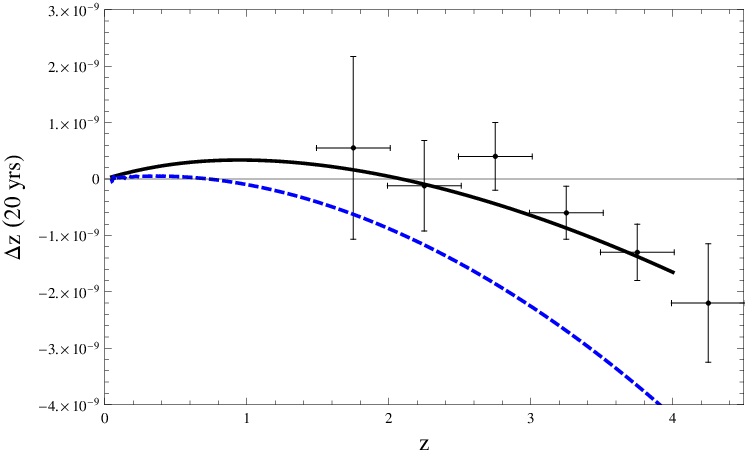
Figure 2 compares the expected time drifts of the cosmological redshift for the LTB- and FL-models. $\Delta z=\dot{z}\Delta t_{\rm obs}$ has a typical amplitude of order $10^{-9}$ on a time scale of $\Delta t_{\rm obs}=20$ yr, for a source at redshift $z\sim 4$ . This measurement is impossible with present-day facilities. However, it was recently revisited [25] in the context of ELT, arguing they could measure velocity shifts of order $1Ð10$ cm/s over a 10 yr period from the observation of the Lyman- $\alpha$ forest. It is one of the science drivers in design of the CODEX ultrastable spectrograph [26] for the future European ELT. Indeed, many effects, such as proper motion of the sources, local gravitational potential, or acceleration of the Sun may contribute to the time drift of the redshift. It was shown [27, 28], however, that these contributions can be brought to a 0.1% level so that the cosmological redshift is actually measured. The data points and error bars of Fig. 2 follows the forecast of Ref. [26]. Our analysis confirms the recent analysis by Ref. [29], which also suggests to use the cosmic parallax.

II.5 Discussion

The result of Fig. 2 demonstrates that the information off the light-cone allows to distinguish a $\Lambda$ -CDM from a LTB-model specially designed to have the same luminosity (or angular) distance redshift relation and the same mass density-redshift relation as the a $\Lambda$ -CDM. In the case of a dark energy model both $D_{L}(z)$ and $\dot{z}$ are modified, and little insight is gained on the equation of state from adding the new information on $\dot{z}$ [30]. The case of the large scale inhomogeneity turns out to be different and the $\dot{z}$ observation would provide, when available, an interesting extra-test of these models that cannot be performed otherwise.

Indeed, Fig. 2 was obtained by forcing $D_{A}(z)$ to match the $\Lambda$ CDM prediction up to $z\simeq 4$ while SNIa data [2] extend roughly to $z\sim 1.6$ . Following e.g. Ref. [31], one can try to design density profiles such that the LTB model reproduces the $\Lambda$ CDM- $D_{A}(z)$ at low redshift and becomes homogeneous on large scales. Note that reproducing $\rho$ and $D_{A}$ of a flat- $\Lambda$ CDM imposes that $H_{\perp}(z)=H_{FL}(z)$ . Now, assuming that it fits $\dot{z}_{FL}$ and $\rho$ at high redshift implies that $H_{\perp}=H_{\parallel}=H_{FL}$ . While attractive, such models seem however difficult to construct since they usually require that $M^{\prime}<0$ between these two regimes.

This example demonstrates the complementarity of these two observables since they concern two domains of redshift. To go further in distinguishing such a model from its FL-twin, we shall now consider the influence of the large scale inhomogeneity on the growth of large scale structures.

III Evolution of density perturbation in a LTB universe

A general study of the perturbation theory around a LTB background was performed using a coordinate based approach in Ref. [32], and the general features of the growth of density perturbations were discussed in Ref. [33]. The goal of this section is to investigate the evolution of the density contrast using the 1+1+2 formalism, and to obtain an approximation for the evolution equations. We also discuss how the density contrast variable introduced here can be related to observations.

III.1 General formalism

III.1.1 1+3 formalism

In the 1+3 covariant approach [34], in which one introduces the worldline tangent vector $u^{a}$ ( $u^{a}u_{a}=-1$ ), one first introduces the projection tensor $h^{a}{}_{b}\equiv\delta^{a}{}_{b}+u^{a}u_{b}$ . This projection tensor defines two derivatives for any tensor ${T}^{a}{}_{b}$ , the covariant time derivative along the fundamental worldlines

\dot{T}^{a}{}_{b}\equiv u^{e}\nabla_{e}T^{a}{}_{b}\,,

(29)

and the fully projected covariant derivative $D_{e}$ via

D_{e}T^{a}{}_{b}\equiv h^{a}{}_{f}\,h^{g}{}_{b}\,h^{r}{}_{e}\nabla_{r}\,T^{f}{}_{g}\ ,

(30)

where we fully project on all free indices.

The projection tensor $h_{ab}$ allows for any 4-vector to be split into a scalar part parallel to $u^{a}$ and a 3-vector part orthogonal to $u^{a}$ . Similarly, any second rank tensor may be covariantly and irreducibly split into scalar, vector and projected, symmetric, trace-free (PSTF) 3-tensor parts.

We can also split the covariant derivative of $u_{a}$ into its irreducible parts as

	$\displaystyle\nabla_{a}u_{b}$	$\displaystyle=$	$\displaystyle-\,u_{a}\,\dot{u}_{b}+D_{a}u_{b}$		(31)
		$\displaystyle=$	$\displaystyle-\,u_{a}\,\mathcal{A}_{b}+{{\textstyle{1\over 3}}}\,\Theta\,h_{ab}+\sigma_{ab}+\omega_{ab}\,.$		(32)

This uniquely defines the following kinematic quantities: $\mathcal{A}_{b}=\dot{u}_{b}$ is the acceleration, the trace $\Theta=D_{a}u^{a}{}$ is the (volume) rate of expansion of the fluid (with $H=\Theta/3$ the Hubble parameter), $\sigma_{ab}=D_{\langle a}u_{b\rangle}$ is the trace-free symmetric rate of shear tensor describing the rate of distortion of the matter flow, and $\omega_{ab}=D_{[a}u_{b]}$ is the skew-symmetric vorticity tensor, describing the rotation of the matter relative to a non-rotating frame. It is also useful define a scale factor $a$ along the fundamental worldlines via

\frac{\dot{a}}{a}=\frac{1}{3}\,\Theta\,.

(33)

III.1.2 1+1+2 formalism

We now employ the 1+1+2 formalism [35], that builds on the 1+3 formalism by allowing a further “spatial” slicing with respect to a spacelike unit vector field $n^{a}$ , which is orthogonal to the timelike 4-velocity vector ( $u^{a}n_{a}=0$ ). The 1+3 projection tensor ${h_{a}}^{b}$ combined with $n^{a}$ gives rise to a new projection tensor ${N_{a}}^{b}$ , which projects vectors and tensors onto the 2-surfaces orthogonal to $n^{a}$ and $u^{a}$ that are referred to as the ‘sheets’:

\displaystyle N^{a}{}_{b}\equiv h^{a}{}_{b}-n^{a}n_{b}=g^{a}{}_{b}+u^{a}u_{b}-n^{a}n_{b}\,.

(34)

Analogously to the 1+3 formalism, $N_{a}{}^{b}$ defines two new derivatives for any object $T_{\cdots}{}^{\cdots}$ :

	$\displaystyle\left({T}^{a}{}_{b}\right)^{\prime}$	$\displaystyle\equiv$	$\displaystyle n^{e}D_{e}T^{a}{}_{b}\,,$		(35)
	$\displaystyle d_{e}T^{a}{}_{b}$	$\displaystyle\equiv$	$\displaystyle N^{a}{}_{f}\,N^{g}{}_{b}\,N^{r}{}_{e}D_{r}\,T_{f}{}^{g}\,.$		(36)

The ^′-derivative is the (spatial) derivative along the vector field $n^{a}$ in the surfaces orthogonal to $u^{a}$ analogous to the time derivative defined in (29), and the $d_{e}$ -derivative is the projected derivative on the sheet analogous to the projected derivative $D_{e}$ defined in (30) ¹¹ 1 Note that the ^′-derivative was denoted by a hat ( $\hat{}$ ), and the $d_{e}$ was denoted $\delta_{e}$ in Ref. [35].. See Ref. [35] for a detailed presentation of the 1+1+2 formalism and the appendix for a summary of the key equations.

III.1.3 The LTB case

For a LTB spacetime all vectors and tensors as well as vorticity, acceleration and the magnetic part of the Weyl tensor vanish at background level. It can be further shown that the expansion, the only non-vanishing component of the shear $\Sigma=n^{\mu}n^{\nu}\sigma_{\mu\nu}$ and of the electric part of the Weyl tensor ${\cal E}=n^{\mu}n^{\nu}E_{\mu\nu}$ are given by

\Theta=2H_{\perp}+H_{\parallel},\quad\Sigma=\frac{2}{3}\left(H_{\perp}-H_{\parallel}\right),

(37)

and

{\cal E}=\frac{8\pi G\rho}{3}-\frac{M}{R^{3}}.

(38)

We depict their evolution on the past light-cone in Fig. 3, and they satisfy the following general evolution equations:

$\displaystyle\dot{\rho}$	$\displaystyle=$	$\displaystyle-\Theta\rho,\$	(39)
$\displaystyle\dot{\Theta}$	$\displaystyle=$	$\displaystyle-\frac{1}{3}\Theta^{2}-4\pi G\rho-\frac{3}{2}\Sigma^{2},$	(40)
$\displaystyle\dot{\Sigma}$	$\displaystyle=$	$\displaystyle-\left(\frac{2}{3}\Theta+\frac{1}{2}\Sigma\right)\Sigma-{\cal E},$	(41)
$\displaystyle\dot{\cal E}$	$\displaystyle=$	$\displaystyle-\left(\Theta-\frac{3}{2}\Sigma\right){\cal E}-4\pi G\rho\Sigma.$	(42)

III.2 The density perturbation equations

We can decompose the standard dimensionless normalized density gradient ${\cal D}_{a}\equiv a~h_{ab}\nabla^{b}\rho/{\rho}$ into a part $\Delta_{a}$ that lies in the sheet and a part perpendicular to the sheet:

\displaystyle{\cal D}_{a}=a\frac{{\rho}^{\prime}}{\rho}n_{a}+a\frac{d_{a}\rho}{\rho}\equiv\,a\frac{{\rho}^{\prime}}{\rho}n_{a}+\Delta_{a}\,,

(43)

where we recall that $\rho^{\prime}=n^{b}D_{b}\rho$ and $d_{a}\rho=N^{b}{}_{a}D_{b}\rho$ .

It is clear that $\Delta_{a}$ is gauge-invariant as it vanishes in the background LTB model. To see more clearly what this variable physically represents, let us define an infinitesimal vector $\delta x_{\bar{a}}\equiv N^{b}{}_{a}\,\delta x_{b}$ connecting two neighboring points on the sheet. It follows that the density evaluated at two neighboring points are related by

\displaystyle\rho(x_{a}+\delta x_{\bar{a}})=\rho(x_{a})+d_{a}\rho\,\,\delta x^{\bar{a}}\,.

(44)

In this way we can define a gauge-invariant density contrast $\delta$ :

\displaystyle\delta\equiv\frac{\rho(x_{a}+\delta x_{\bar{a}})-\rho(x_{a})}{\rho(x_{a})}=\frac{1}{a}\Delta_{a}\delta x^{\bar{a}}\,.

(45)

Defining the auxiliary perturbation variables in the sheet

\displaystyle\delta\Theta=\frac{1}{a}\Theta_{a}\delta x^{\bar{a}},\quad\delta\Sigma=\frac{1}{a}\mathcal{T}_{a}\delta x^{\bar{a}},\quad\delta{\cal E}=\frac{1}{a}\mathcal{S}_{a}\delta x^{\bar{a}},

(46)

where

\displaystyle\Theta_{a}=a\,d_{a}\Theta\,,~\mathcal{T}_{a}=a\,d_{a}\Sigma\,,~\mathcal{S}_{a}=a\,d_{a}{\cal E}\,,

(47)

we can derive a set of 4 gauge invariant perturbation equations (neglecting the magnetic part of the Weyl tensor)

$\displaystyle\dot{\delta}$	$\displaystyle=$	$\displaystyle-\delta\Theta+\frac{\rho^{\prime}}{\rho}C_{\bar{a}}\delta x^{\bar{a}}$	(48)
$\displaystyle\left({\delta\Theta}\right)\dot{}$	$\displaystyle=$	$\displaystyle-\frac{2}{3}\Theta\delta\Theta-4\pi G\rho\delta-3\Sigma\delta\Sigma$	(49)
		$\displaystyle-\Theta^{\prime}C_{\bar{a}}\delta x^{\bar{a}}$	(49)
$\displaystyle\left({\delta\Sigma}\right)\dot{}$	$\displaystyle=$	$\displaystyle\left(-\frac{2}{3}\Theta-\Sigma\right)\delta\Sigma-\frac{2}{3}\Sigma\delta\Theta-\delta{\cal E}$	(50)
		$\displaystyle-\Sigma^{\prime}C_{\bar{a}}\delta x^{\bar{a}}$	(50)
$\displaystyle\left({\delta\cal E}\right)\dot{}$	$\displaystyle=$	$\displaystyle-\left(\Theta-\frac{3}{2}\Sigma\right)\delta{\cal E}+\left(\frac{3}{2}{\cal E}-4\pi G\rho\right)\delta\Sigma$	(51)
		$\displaystyle-{\cal E}\delta\Theta-4\pi G\rho\Sigma\delta-{\cal E}^{\prime}C_{\bar{a}}\delta x^{\bar{a}}\,,$	(51)

where $C_{\bar{a}}=\Sigma_{\bar{a}}+\alpha_{\bar{a}}$ . The equation for the connecting vector $\delta x^{\bar{a}}$ is only needed to background order,

\displaystyle\delta\dot{x}^{\bar{a}}=\frac{1}{2}\left(\frac{2}{3}\Theta-\Sigma\right)\delta x^{\bar{a}}\,.

(52)

The set of equations (48-52) provides a complete description of the evolution of the gauge invariant density contrast in situations where the magnetic part of the Weyl tensor can be neglected. This ‘silent” approximation can be thought of as neglecting the coupling between density perturbations and gravitational waves in pressure-free models and has been widely studied in the context of non-linear gravitational collapse [52].

The above equations can be solved iteratively as follows. Expanding the perturbation variables in the form $\delta X^{i}=\delta X_{0}+f^{i}_{\bar{a}}\delta x^{\bar{a}}$ , (with $i=1\ldots 4$ and the short-hand notation $\delta X^{1}=\delta$ etc.), we obtain a set of homogeneous equations for the leading part of the perturbations

$\displaystyle\dot{\delta}_{0}$	$\displaystyle=$	$\displaystyle-\delta\Theta_{0}$	(53)
$\displaystyle\left({\delta\Theta}\right)\dot{}_{0}$	$\displaystyle=$	$\displaystyle-\frac{2}{3}\Theta\delta\Theta_{0}-4\pi G\rho\delta-3\Sigma\delta\Sigma_{0}$	(54)
$\displaystyle\left({\delta\Sigma}\right)\dot{}_{0}$	$\displaystyle=$	$\displaystyle\left(-\frac{2}{3}\Theta-\Sigma\right)\delta\Sigma_{0}-\frac{2}{3}\Sigma\delta\Theta_{0}-\delta{\cal E}_{0}$	(55)
$\displaystyle\left({\delta\cal E}\right)\dot{}_{0}$	$\displaystyle=$	$\displaystyle-\left(\Theta-\frac{3}{2}\Sigma\right)\delta{\cal E}_{0}+\left(\frac{3}{2}{\cal E}-4\pi G\rho\right)\delta\Sigma_{0}$	(56)
		$\displaystyle-{\cal E}\delta\Theta-4\pi G\rho\Sigma\delta_{0}\,,$	(56)

with the corrections evolving according to equations of the form

\displaystyle\dot{f}^{i}_{\bar{a}}=-\frac{1}{2}\left(\frac{2}{3}\Theta-\Sigma\right)f^{i}_{\bar{a}}+\alpha^{i}C_{\bar{a}}\,

(57)

with $\alpha^{i}\equiv(\rho^{\prime}/\rho,-\Theta^{\prime},-\Sigma^{\prime},-{\cal E}^{\prime}$ ). The homogeneous equations can then be combined to give a pair of coupled second order equations

$\displaystyle\ddot{\delta}_{0}$	$\displaystyle+$	$\displaystyle\frac{2}{3}\Theta\dot{\delta}_{0}-4\pi G\rho\delta_{0}=3\Sigma\delta\Sigma_{0}\,,$	(58)
$\displaystyle\left({\delta\Sigma}\right)\ddot{}_{0}$	$\displaystyle+$	$\displaystyle(\frac{5}{3}\Theta-\frac{1}{2}\Sigma)\left({\delta\Sigma}\right)\dot{}_{0}$	(59)
	$\displaystyle-$	$\displaystyle\left(\frac{20}{3}\pi G\rho+\frac{2}{3}\Theta\Sigma-\frac{4}{9}\Theta^{2}-\frac{1}{2}{\cal E}+5\Sigma^{2}\right)\delta\Sigma_{0}$
	$\displaystyle=$	$\displaystyle-\left(\frac{4}{3}\Sigma^{2}+\frac{2}{3}{\cal E}+\frac{2}{9}\Sigma\Theta\right)\dot{\delta}_{0}+\frac{20}{3}\pi G\rho\delta_{0}\,.$

The first one is similar to the standard one in FL models, but with a source term proportional to the background and perturbed shear so that it is coupled to a second differential equation for $\delta\Sigma_{0}$ .

In the cases where the above approximations are not valid, one needs to consider the considerably more complex full set of 1+1+2 equations that is described in the appendix.

IV Transfer functions and initial conditions

IV.1 Back to Friedmann-Lemaître spacetime

Before investigating the growth of structure in a LTB universe, let us recall the relations between the background dynamics and the growth of large scale structure in a flat $\Lambda$ CDM model.

Since the cosmological constant develops no perturbation, and since the growth of the density perturbations of the pressureless CDM component is dictated by general relativity, it implies that in the linear regime, the evolution equations reduce to the two equations

\dot{\delta}=-\delta\Theta,\qquad\delta\dot{\Theta}=-2H_{FL}\delta\Theta-4\pi G\rho\delta\,,

(60)

that is to

\ddot{D}+2H\dot{D}-4\pi G\rho_{\rm m}D=0,

(61)

where the CDM density contrast has been decomposed as $\delta({\bf x},t)=D_{+}(t)\varepsilon_{+}({\bf x})+D_{-}(t)\varepsilon_{-}({\bf x})$ , $\varepsilon_{\pm}$ encoding the initial conditions. This equation can be recast in terms of $a$ as time variable [36, 37] as

D^{\prime\prime}+\left(\frac{{\rm d}\ln H}{{\rm d}a}+\frac{3}{a}\right)D^{\prime}=\frac{3}{2}\frac{\Omega_{{\rm m}0}}{a^{5}}D.

(62)

Since $D_{-}=H$ is a solution, the growing mode is given by

\displaystyle D_{+}

\displaystyle=

\displaystyle\frac{5}{2}\frac{H(z)}{H_{0}}\Omega_{{\rm m}0}\int_{z}^{\infty}\frac{(1+z^{\prime}){\rm d}z^{\prime}}{[H(z^{\prime})/H_{0}]^{3}}.

(63)

In our particular case, this can be integrated analytically as

	$\displaystyle D_{+}(z)$	$\displaystyle\propto$	$\displaystyle{}_{2}F_{1}\left[1,\frac{1}{3};\frac{11}{6};-\left(\frac{1-\Omega_{{\rm m}0}}{\Omega_{{\rm m}0}}\right)\frac{1}{(1+z)^{3}}\right]$		(64)
			$\displaystyle\times\left(\frac{1-\Omega_{{\rm m}0}}{\Omega_{{\rm m}0}}\right)^{1/3}\frac{1}{1+z}.$		(64)

This implies that if $H(z)$ is known from background observations, such as SNIa, then $D_{+}(z)$ is fixed and is thus not an independent quantity in this framework. There is a rigidity between the expansion history of the background and the growth rate [36, 38]. This has attracted attention since this offers a test of the $\Lambda$ CDM model [39, 40]. Moreover, Eq. (60) implies that $\vartheta\equiv\delta\Theta/H$ is related to the density contrast by

\vartheta=-f(a)\delta

(65)

where the function $f$ can be parameterized as [41, 42]

f_{+}\equiv\frac{{\rm d}\ln D_{+}}{{\rm d}\ln a}=\Omega_{\rm m}(a)^{\gamma}

(66)

for the growing mode. Then, if general relativity is not modified, the index $\gamma$ can be computed once $H(z)$ , or equivalently the dark energy equation of state, is known and it was shown [43, 44] that $\gamma=0.55$ in the case of a $\Lambda$ CDM. Since $\gamma$ can be measured from galaxy redshift surveys [46], thanks to the redshift distortion [45], it was argued that the value of the parameter $\gamma$ offers a test of general relativity [39].

IV.2 Structure of the LTB growth rate equations

In a LTB spacetime, and under the approximations discussed in Section III, we need to solve a set of 4 differential equations that can be recast as

\dot{X}_{i}=M_{ij}(r,t)X_{j},

(67)

where $X_{i}=(\delta,\delta\Theta,\delta\Sigma,\delta{\cal E})$ and where the matrix $M_{ij}$ depends only on $r$ and $t$ through the background quantities $\Theta$ , $\Sigma$ , $\rho$ and ${\cal E}$ . It follows that the general solution is of the form

X_{i}(r,t,\theta,\varphi)=T_{ij}(r,t)X_{j}(r,t_{\rm init},\theta,\varphi)

(68)

where the angular dependence stems only from the initial conditions so that the transfer functions depends only on $r$ and $t$ . When interested in observations such as weak-lensing, one integrates along the light-cone so that only $T_{ij}(z)=T_{ij}[r_{*}(z),t_{*}(z)]$ is actually needed (see Ref. [33]).

IV.2.1 Integrating the perturbation equations

In order to compute the transfer functions, we proceed as follows (see Fig. 4).

•

Using the reconstruction along the past light-cone, we integrate for each $z$ the background equations (39-42) from $t=t_{0}-r_{*}(z)$ toward the interior of the past light-cone at $r=r_{*}(z)$ constant. This provides the background quantities $\rho(t,r)$ , $\Theta(t,r)$ , $\Sigma(t,r)$ , and ${\cal E}(t,r)$ for this particular $r$ in agreement with the constraint that $R=D_{A}$ and $\rho=\rho_{FL}$ on the past light-cone.
•

We then solve the perturbation equations with this background functions from an initial time $t_{\rm init}$ up to $t_{*}(z)$ considering the four sets of initial conditions:

$X_{i}^{(\alpha)}(r,t_{\rm init},\theta,\varphi)=\delta_{i}^{\alpha},\qquad\alpha=1\ldots 4.$ (69)

For each set $\alpha$ , we obtain 4 transfer functions $T_{i\alpha}$ .

Such an integration procedure is made possible because the background equations involve no gradient term, so that each shell of constant $r$ evolves independently and because, in the silent approximation used in this work, the perturbation equations enjoy the same property. In this approximation, the spatial inhomogeneity of the background spacetime reflects itself only on the fact that a structure observed at a redshift $z$ had a growth history along the shell $r=r_{*}(z)$ which is different from the other shell. This is a major difference with the FL situation in which, as soon as we are dealing with a pressureless fluid, all the structures have the same growth rate from $z$ to 0, independently of their growth rate at higher redshift.

First, this procedure can be tested on the FL model for which $\Sigma=0$ so that $(\delta,\delta\Theta)$ decouples from $(\delta\Sigma,\delta{\cal E})$ . Focusing on the matter density contrast $\delta$ , we compute the two transfer functions $T_{\rho\rho}$ and $T_{\rho\theta}$ corresponding respectively to the initial conditions $(\delta,\delta\Theta)=(1,0)$ and $(\delta,\delta\Theta)=(0,1)$ . None of these transfer functions corresponds to the growing mode (63) that is obtained from the initial conditions $(\delta,\delta\Theta)=(1,-f_{+}(t_{\rm init})H_{\rm init})$ so that

D_{+}(z)=T_{\rho\rho}(z)-f_{+}(t_{\rm init})H_{\rm init}T_{\rho\theta}(z).

(70)

Figure 5 shows that this is actually verified numerically. Note that even though we reduce the dimension of the space of initial conditions by picking up the growing mode, we still need the two transfer functions. Indeed one can also check that $\delta\theta_{+}(z)=T_{\theta\rho}(z)-f_{+}(t_{\rm init})H_{\rm init}T_{\theta\theta}(z)=-Hf_{+}\delta_{+}$ .

IV.2.2 Initial conditions

To compute the transfer functions of the LTB model, we need to specify an initial spatial hypersurface. Any 3-dimensional spacelike hypersurface $\{r=t_{\rm init}(r)\}$ is a priori possible but three choices can be argued to be natural: (i) a constant time hypersurface, (ii) a constant density hypersurface or (iii) a constant $t-t_{B}(r)$ , i.e. a constant proper time after the big bang. Indeed, in a FL model, these three possibilities reduce to the same hypersurface.

For the purpose of the illustration, we decide to set the initial conditions on a constant time hypersurface, as in Ref. [33], but we cannot justify this choice further here. Then, applying the procedure described in Section IV.2.1, we obtain the transfer functions. Figure 6 describes the four transfer functions needed to compute the density contrast on the past light-cone.

IV.2.3 Comparison of the two models

With the previous prescription, the two transfer functions $T_{\rho\rho}$ and $T_{\rho\delta}$ for the two models look similar in shape and amplitude.

To compare the growth rate, one needs to know the initial conditions, or at least the relative initial value of $\delta$ , $\delta\Theta$ , $\delta\Sigma$ and $\delta{\cal E}$ . As we have seen in Section IV.2.1, a particular choice of $(\delta,\delta\Theta)$ allows to pick up the growing mode. We have no indication of the linear combination of the transfer functions that are related to the growing mode in the LTB case. In order to compare the growth rate, we assume that at early time the universe was well described by a FL-model and that the void evolves at lower redshift. In such a case, the initial conditions can be set by their FL analog for the growing mode. From Eqs. (104) and (107), we deduce that

\frac{1}{2}\Theta\delta\Sigma_{\rm init}=\frac{2}{3}(8\pi G\delta\rho_{\rm init}),\quad\frac{1}{2}\delta{\cal E}_{\rm init}=-\frac{8\pi G}{3}\delta\rho_{\rm init}

(71)

and for the growing mode

\delta\Theta_{\rm init}=-f_{+}({\rm init})H({\rm init})\delta_{\rm init}.

(72)

That would imply that $\delta=D_{+}^{\rm LTB}\delta_{i}$ with

	$\displaystyle D_{+}^{\rm LTB}(z)$	$\displaystyle=$	$\displaystyle T_{\rho\rho}(z)-f_{+}({\rm init})H({\rm init})T_{\rho\theta}(z)$		(73)
		$\displaystyle+$	$\displaystyle(8\pi G\rho_{\rm init})\left[\frac{4}{9H_{\rm init}}T_{\rho\Sigma}(z)-\frac{2}{3}T_{\rho{\cal E}}(z)\right].$		(73)

It corresponds to the growing mode of the density perturbation if the universe has evolved from a FL-phase and if the density perturbations had time to reach the FL growing mode before the effect of the void on the evolution of the perturbations starts being non-negligible. Indeed, we have no proof that it is the growing mode of the LTB-system. 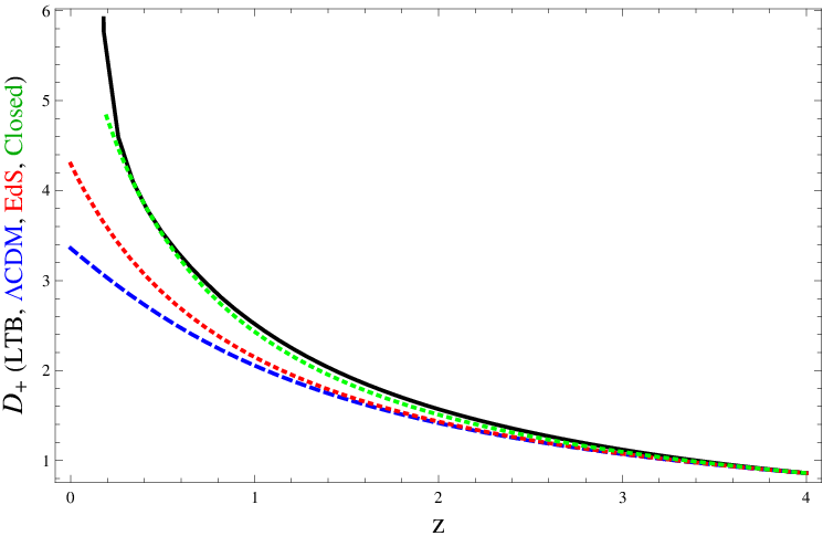Note that the 4 transfer functions are needed to described the evolution of the density, even though the initial conditions can be reduced to the single random variable $\delta_{\rm init}(r,t_{\rm init},\theta,\varphi)$ .

Fig. 7 compares this solution to the growing mode of various FL-models. All models are normalized at high redshift, and we can see that the LTB-model has more structure at small redshift and that its growth rate is qualitatively similar to the one of a closed FL-model. We can also note that it seems impossible to find a linear combination of the 4 transfer functions that would mimic the growth rate of the $\Lambda$ CDM model. This is an interesting conclusion, given our ignorance of the initial conditions. Indeed, in general, we expect the initial conditions to be not simply a linear combination but of the form

\delta\Theta_{\rm init}=f_{\Theta}(r)\delta_{\rm init}(r,\theta,\varphi),\quad\delta\Sigma_{\rm init}=f_{\Sigma}(r)\delta_{\rm init}(r,\theta,\varphi),

(74)

and

\delta{\cal E}_{\rm init}=f_{\cal E}(r)\delta_{\rm init}(r,\theta,\varphi),\qquad

(75)

that is involving three arbitrary functions of $r$ . Unless we have theoretical constraints of $f_{\Theta}$ , $f_{\Sigma}$ and $f_{\cal E}$ , the growth rate (73) can be tuned at will. It follows that the determination of the growth rate is more likely to teach us on the initial conditions than to be used as an extra-data for the reconstruction program.

As emphasized, in the $\Lambda$ CDM, the growth rate and the background dynamics are not independent so that we have relation such as Eq. (66). For the $\Lambda$ CDM, $\gamma=0.55$ and slight deviation from this value are expected for dark energy models in which general relativity is not modified [39]. The index

\varepsilon(a)=\left[\Omega_{\rm m}(a)\right]^{-\gamma}\frac{{\rm d}\ln D}{{\rm d}\ln a}-1,

(76)

introduced in Ref. [40] should not deviate significantly from 0. $\gamma$ and $\Omega_{\rm m}$ are determined from background observations and thus coincide with their $\Lambda$ CDM values. It was shown that $\varepsilon$ can typically vary between 0.05 and 0.25 for modification of general relativity of the $f(R)$ -class [40]. Using the numerical solution corresponding to Fig. 7, we estimate that $\varepsilon$ can reach 0.1. The deviation arises from the fact that the perturbation equations involve the shear and the electric part of the Weyl tensor and indeed not from a deviation from general relativity. This illustrates that it is indeed important to ensure the validity of the Copernican principle when applying tests of general relativity based on the large scale structures since they usually implicitly assume its validity.

To finish, let us also emphasize that any observable, ${\cal O}$ say, entangles the properties of the transfer functions and of the initial conditions. In general, it can be written as an integral along the line of sight as

{\cal O}(z,n^{a})=\int_{0}^{z}w(z,z^{\prime})\delta[x^{\mu}(z^{\prime},n^{a})]{\rm d}z^{\prime},

where $\delta$ stands for some combination of the perturbation variables and $w$ for some window function that depends on the observable (e.g. for weak lensing in a FL universe $\delta$ will correspond to twice the gravitational potential and $w$ can be expressed in terms of angular distances). In a Friedmann-Lemaître universe, as long as we focus on the evolution of dark matter, we have that $\delta(x^{i},t)=T(t)\delta_{\rm init}(x^{i})$ so that the correlation function of ${\cal O}$ takes the form

	$\displaystyle\langle{\cal O}(z,n_{1}^{a}){\cal O}(z,n_{2}^{a})\rangle=\int_{0}^{z}\!\!{\rm d}z^{\prime}\int_{0}^{z}\!\!{\rm d}z^{\prime\prime}w(z,z^{\prime})w(z,z^{\prime\prime})$
	$\displaystyle T(z^{\prime})T(z^{\prime\prime})\xi_{\rm init}(\sqrt{r^{2}(z^{\prime})+r^{2}(z^{\prime\prime})-2r(z^{\prime})r(z^{\prime\prime})\cos\theta}),$

with $\cos\theta=n_{1}.n_{2}$ and where the correlation function of the initial condition, $\xi_{\rm init}$ is a function of $|x^{i}_{1}-x^{i}_{2}|$ only because of isotropy and homogeneity. This integral is usually easily evaluated in Fourier space. On small scales, the initial conditions decouple from the evolution mainly because the power is mainly carried by modes perpendicular to the line of sight (which is at the basis of the Limber approximation) but the initial power spectrum has to be such as this property holds, which is the case for an almost scale invariant power spectrum. In a LTB universe, there are two main differences with the FL case. First the transfer functions depend on $r$ and $t$ so that $\delta(x^{i},t)=T(r,t)\delta_{\rm init}(x^{i})$ and second the initial correlation dunction is a function $\xi_{\rm init}(r(z^{\prime}),r(z^{\prime\prime}),\cos\theta)$

	$\displaystyle\langle{\cal O}(z,n_{1}^{a}){\cal O}(z,n_{2}^{a})\rangle=\int_{0}^{z}\!\!{\rm d}z^{\prime}\int_{0}^{z}\!\!{\rm d}z^{\prime\prime}w(z,z^{\prime})w(z,z^{\prime\prime})$
	$\displaystyle\qquad T[r(z^{\prime}),t(z^{\prime})]T[r(z^{\prime\prime}),t(z^{\prime\prime})]\xi_{\rm init}[r(z^{\prime}),r(z^{\prime\prime}),\cos\theta].$

It follows that the spatial dependency of the transfer functions mixes with the one of the initial conditions and that we cannot ensure a priori that a condition similar to the Limber property will exist.

Indeed, once a theory of the initial conditions compatible with the origin of a large scale inhomogeneity exist, one can use our analysis to compute the angular power spectrum of the observable ${\cal O}$ . While being focused on the properties of the transfer functions, our work however show that if $\xi_{\rm initi}$ is identical as in a FL universe then the effect of the evolution can lead to significant effect.

V Discussion

In this article, we have used a LTB model that mimics a FL model on the past light-cone in order to shown that these two models can still be distinguished by background observations that encode information “off” the light-cone, as for instance the time drift of cosmological redshift. While such an observation was advocated as a test of the Copernican principle in Ref. [10], the amplitude of the difference with the $\Lambda$ CDM prediction had not been estimated. We have shown that it can be significant and that it can allow to exclude a large class of LTB models even though they look similar to FL models at the background level.

Then, we investigated the information that can be extracted from large scale structure. Assuming that the curl of the magnetic part of the Weyl tensor can be neglected, we have shown that one can extract a closed system of 4 perturbation equations. Our derivation clarifies the link with the gauge invariant variables of the $1+1+2$ formalism. On small angular scales, we argued that one can make a silent approximation. Under such conditions, our set of equations for scalar perturbations reduce to the ones used in Ref. [33].

We have detailed a procedure to compute the transfer functions of this system of perturbation equation, once the background data is known on the past light-cone and we explained how the corrections at first order in the connecting vector can be obtained. We emphasized the difficulty in determining a set of the initial conditions, i.e. to define the hypersurface on which they are defined and the relation that could exist between the different modes (in particular to extract the growing mode).

Indeed, our discussion of the perturbation dynamics is more illustrative than quantitative for two reasons. The first one is mainly technical since we have used the silent approximation instead of solving the full set of 1+1+2 equations. This can only be achieved numerically and is left for further investigation. The second is related to an intrinsic limitation concerning our ignorance of the initial conditions: (1) we do not know the hypersurface on which they have to be specified and (2) while we have been able to compute the transfer function, we are not able to specify their exact combination that corresponds to the growing mode. While in a FL universe, the late behaviour of the growth function of dark matter reduces to a function of time, or equivalently of redshift, it is in the LTB case a function of $t$ and $r$ that reduces to a function of $z$ on the light-cone. This implies a further limitation since the large scale structure properties strongly entangle the evolution and the initial conditions. It is thus difficult to close the reconstruction program unless we have some constraints on the initial condition. Nevertheless, our investigation shows that we cannot find a linear combination (with constant coefficients) of the transfer functions that reproduce the growing mode of the $\Lambda$ CDM. It also illustrates explicitely one limitation of the tests of general relativity based on the large scale structure (e.g. the $\gamma$ -index is difficult to generalize to a LTB spactime because Eqs. (65-66) have to be reconsidered).

This emphasizes the importance to test the Copernican principle to validate the test of general relativity based on the properties of large scale structures and illustrates the effect of the assumption on the large scale geometry of our universe on these tests. In that respect both the time drift of the cosmological redshifts and the growth of density perturbations give access to the spacetime structure beyond the light-cone and are thus key observations for our understanding of the geometry of our universe.

Acknowledgements.

We thank C. Clarkson, G.F.R Ellis and Y. Mellier for useful discussions and comments.

References

[1] D.N. Spergel et al. Astrophys. J. Suppl. 148, 175 (2003).
[2] S. Perlmutter et al., Astrophys. J. 517, 565 (1999); A.G. Riess et al., Astron. J. 116, 1009 (1998); J.L. Tonry et al., Astrophys. J. 594, 1 (2003); R.A. Knop et al., Astrophys. J. 598, 102 (2003); A.G. Riess et al. Astrophys. J. 607, 665 (2004).
[3] M. Tegmark et al., Phys. Rev. D 69, 103501 (2004); U. Seljak et al., Phys. Rev. D 71, 103515 (2005).
[4] D.J. Eisenstein et al., Astrophys. J. 633, 560 (2005).
[5] L. Fu et al., Astron. Astrophys. 479, 9 (2008).
[6] J.-P. Uzan, Gen. Rel. Grav. 39, 307 (2007).
[7] J.-P. Uzan, Dark energy, gravitation and the Copernican principle, in Dark energy, P. Ruiz Lapuente Ed., (Cambridge University Press, 2010), arXiv:0912.5452.
[8] J.-P. Uzan, Gen. Rel. Grav. (to appear), arXiv:0908.2243.
[9] B. Ratra and P. J. E. Peebles, Rev. Mod. Phys. 75, 559 (2003).
[10] J.-P. Uzan, C.C. Clarkson, and G.F.R. Ellis, Phys. Rev. Lett. 100, 191303 (2008).
[11] J. Goodman, Phys. Rev. D 52, 1821 (1995); R.R. Caldwell and A. Stebbins, Phys. Rev. Lett. 100, 191302 (2008).
[12] C. Clarkson, B. Bassett, and T. Lu, Phys. Rev. Lett. 101, 011301 (2008).
[13] A.E. Romano, JCAP 01, 004 (2010); A.E. Romano, Phys. Rev. D 76, 103525 (2007).
[14] N. Mustapha et al., Mon. Not. R. Astron. Soc. 292, 817 (1997).
[15] M. Célérier, Astron. Astrophys. 353, 63 (2000).
[16] H. Iguchi, T. Nakamura, and K.-I. Nakao, Prog. Theor. Phys. 108, 809 (2002).
[17] M. Célérier et al., arXic:0906.0905[astro-ph.CO].
[18] A.E. Romano, 0912.2866.
[19] J. W. Moffat and D. C. Tatarski, Phys. Rev. D 45, 3512 (1992); ibid., arXiv:astro-ph/9404048; N. Sugiura, et al., Phys. Rev. D 60, 103508 (1999); C. H. Chuang, J. A. Gu, and W.Y. Hwang, astro-ph/0512651; D. Garfinkle, Class. Quant. Grav. 23, 4811 (2006); D. J. Chung and A. E. Romano, Phys. Rev. D 74, 103507 (2006); R. A. Vanderveld, et al., Phys. Rev. D 74, 023506 (2006); H. Alnes, et al., Phys. Rev. D 73, 083519 (2006); R. Mansouri, astro-ph/0606703; M. N. Célérier, New Adv. Phys. 1, 29 (2007); K. Enqvist and T. Mattsson, J. Cosmol. Astropart. Phys. 02, 019 (2007); C.-M. Yoo, et al., Progr. Theor. Phys. 120, 937 (2008); J. P. Zibin, et al., Phys. Rev. Lett. 101, 251303 (2008); J. Garcia-Bellido and T. Haugbolle, JCAP 4, 3 (2008); K. Bolejko and J. S. B. Wyithe, JCAP 2, 20 (2009).
[20] G. Lemaître, Ann. Soc. Sci. Bruxelles A 53, 51 (1933); R.C. Tolman, Proc. Nat. Acad. Sci. 20, 169 (1934); H. Bondi, Mon. Not. R. Astron. Soc. 107, 410 (1947).
[21] W. Stoeger, G. F. R. Ellis, and S. Nel, Class. Quant. Grav. 9, 509 (1992); R. Maartens et al., Class. Quant. Grav. 13, 253 (1996); M. E. Araujo and W. R. Stoeger, Phys. Rev. D 60, 104020 (1999).
[22] E.W. Kolb, and C.R. Lamb, arXiv:0911.3852[astro-ph.CO].
[23] C. Clarkson, arXiv:0911.2601[astro-ph.CO].
[24] A. Sandage, Astrophys. J. 136, 319 (1962); G. McVittie, Astrophys. J. 136, 334 (1962).
[25] A. Loeb, Astrophys. J. 499, L111 (1998).
[26] L. Pasquini et al., The Messenger 122, 10 (2005).
[27] J.-P. Uzan, F. Bernardeau, and Y. Mellier, Phys. Rev. D 77, 021301(R) (2008).
[28] J. Liske etal., Mon. Not. R. Astron. Soc. 386, 1192 (2008).
[29] M. Quartin and A. Amensola, arXiv:0909.4954.
[30] P.-S. Corasaniti, D. Huterer, and A. Melchiorri, Phys. Rev. D 75, 062001 (2007); A. Balbi and C. Quercellini, arXiv:0704.235; H. Zhang et al., arXiv:0705.4409.
[31] S. February et al., arXiv:0909.1479[astro-ph.CO].
[32] C. Clarkson, T. Clifton and S. February JCAP 06 (2009) 025
[33] J. P. Zibin Phys. Rev. D 78, 043504 (2008).
[34] G.F.R. Ellis, and H. van Elst, “Cosmological Models”, Cargèse Lectures 1998, in Theoretical and Observational Cosmology, Ed. M Lachièze-Rey, (Dordrecht: Kluwer, 1999), 1. arXiv:gr-qc/9812046; G.F.R. Ellis, and M. Bruni, Phys Rev D 40 1804 (1989); M. Bruni, P.K.S. Dunsby, and G.F.R. Ellis, Astrophys. J. 395 34 (1992); P.K.S. Dunsby, M. Bruni, and G.F.R. Ellis, Astrophys. J. 395, 54 (1992).
[35] C. A. Clarkson, R. K. Barrett, Class. Quant. Grav. 20, 3855 (2003); C. Clarkson et al., Astrophys. J. 613, 492 (2004); C. Clarkson, Phys. Rev. D 76, 104034 (2007).
[36] T. Chiba, and T. Nakamura, Prog. Theor. Phys. 118, 815 (2007); S. Nesseris, S., and L. Perivolaropoulos, Phys. Rev. D 77, 023504 (2008).
[37] P. Peter, P., and J.-P. Uzan, Primordial Cosmology, Oxford University Press, 2009.
[38] E.V. Linder, Astropart. Phys. 29, 336 (2008); Y. Wang, JCAP 0805, 021 (2008).
[39] M. Ishak, M., A. Upadhye, and D.N. Spergel, Phys. Rev. D 75, 043513 (2006); Y. Wang et al., Phys. Rev. D 76, 063503 (2007); M.J. Mortonson, W. Hu, and D. Huterer, Phys. Rev. D 79, 023004 (2009); U. Alam, U., V. Sahni, and A.A. Starobinsky, arXiv:0812.2846.
[40] V. Acquaviva, et al., Phys. Rev. D 78, 043514 (2008);
[41] E.V. Linder, and R.N. Cahn, Astropart. Phys. 28, 481 (2007).
[42] D. Huterer, and E.V. Linder, Phys. Rev. D 75, 023519 (2007).
[43] E.V. Linder, Phys. Rev. D 72, 043529 (2005).
[44] L.M. Wang, and P.J. Steinhardt, Astrophys. J. 508, 483 (1998).
[45] N. Kaiser, Month. Not. R. Astron. Soc. 227, 1 (1987); F. Bernardeau, et al., Phys. Rept. 367, 1 (2002).
[46] M. Tegmark, A.J.S Hamilton, and Y. Xu, Month. Not. R. Astron. Soc. 335, 887 (2002); O. Le Fèvre, et al., Astron. Astrophys. 439, 877 (2005); L. Guzzo, et al., Nature 451, 541 (2008); A. Kosowsky, and S. Bhattacharya., arXiv:0907.4202.
[47] R.K. Sachs, Proc. R. Soc. London A 264, 309 (1961).
[48] P. Schneider, J. Ehlers, and E.E. Falco, Gravitational Lenses (Springer Verlag, Heidelberg, 1992).
[49] R. Kantowski, J. Math. Phys., 9, 336 (1968).
[50] V. Perlick, Living Rev. Relativity 7, 9 (2004).
[51] M. Bartelmann, and P. Schneider, Phys. Rept. 340, 291 (2001).
[52] M. Bruni, S. Matarrese, O. Pantano Astrophys. J. 445, 958 (1995).

Appendix A Full set of perturbation equations in the 1+1+2 formalism

If the magnetic part of the Weyl tensor or the source term $(\Sigma_{a}+\alpha_{a})\delta^{\bar{a}}$ cannot be neglected, the linear perturbations around a LTB background are no longer described by equations (48-52), and the complete set of first order equations below will successively be required to obtain a closed system of linear perturbations.

Let us first recall that in the 1+1+2 framework any 3-vector or PSTF 3-tensor $T_{ab}$ can be irreducibly decomposed with respect to $n^{a}$ into scalar, vector and tensor parts:

T_{ab}={\mathcal{T}}\left(n_{a}n_{b}-{\textstyle\frac{1}{2}}N_{ab}\right)+2{\mathcal{T}}_{(a}n_{b)}+{\mathcal{T}}_{{ab}},

(77)

where

$\displaystyle{\mathcal{T}}$	$\displaystyle\equiv$	$\displaystyle n^{a}n^{b}T_{ab}=-N^{ab}T_{ab},$
$\displaystyle{\mathcal{T}}_{a}$	$\displaystyle\equiv$	$\displaystyle N_{a}^{~b}n^{c}T_{bc},$
$\displaystyle{\mathcal{T}}_{ab}$	$\displaystyle\equiv$	$\displaystyle\left(N_{(a}^{~~c}N_{b)}^{~~d}-{\textstyle\frac{1}{2}}N_{ab}N^{cd}\right)T_{cd}.$	(78)

The shear $\sigma_{ab}$ e.g. will be decomposed into the scalar part $\Sigma=n^{a}n^{b}\sigma_{ab}$ , vector part $\Sigma_{a}=N_{a}^{~b}n^{c}\sigma_{bc}$ and tensor part $\Sigma_{ab}=\left(N_{(a}^{~~c}N_{b)}^{~~d}-{\textstyle\frac{1}{2}}N_{ab}N^{cd}\right)\sigma_{cd}$ .

We may also decompose the covariant derivative of $n^{a}$ orthogonal to $u^{a}$ in analogy to the 1+3 decomposition (31):

D_{a}n_{b}=n_{a}a_{b}+{\textstyle\frac{1}{2}}\phi N_{ab}+\xi\varepsilon_{ab}+\zeta_{ab},

(79)

where

$\displaystyle a_{a}$	$\displaystyle\equiv$	$\displaystyle n^{c}D_{c}n_{a}=n^{\prime}_{a},$	(80)
$\displaystyle\phi$	$\displaystyle\equiv$	$\displaystyle d_{a}n^{a},$	(81)
$\displaystyle\xi$	$\displaystyle\equiv$	$\displaystyle{\textstyle\frac{1}{2}}\varepsilon^{ab}d_{a}n_{b},$	(82)
$\displaystyle\zeta_{ab}$	$\displaystyle\equiv$	$\displaystyle d_{\{a}n_{b\}}.$	(83)

Along the direction $n^{a}$ , $\phi$ represents the sheet expansion, $\zeta_{ab}$ is the shear of $n^{a}$ , $a^{a}$ its acceleration, while $\xi$ represents a ‘twisting’ of the sheet. For the LTB background, $\zeta_{ab},\,n^{a}$ and $\xi$ are first order quantities. Furthermore, we restrict ourselves to perfect fluid perturbations where pressure, 4-acceleration and cosmological constant vanish at all orders.

A.1 Source evolution

The source evolution is then governed by the propagation equations

$\displaystyle\dot{\Sigma}_{a}$	$\displaystyle=$	$\displaystyle-\left(\frac{2}{3}\Theta+\frac{1}{2}\Sigma\right){\Sigma}_{a}-\frac{3}{2}{\Sigma}{\alpha}_{a}-{\mathcal{E}}_{a}$	(84)
$\displaystyle\dot{\cal E}_{\bar{a}}+{\textstyle\frac{1}{2}}\varepsilon_{a}^{b}{\cal H}^{\prime}_{b}$	$\displaystyle=$	$\displaystyle\frac{3}{4}\varepsilon_{ab}d^{b}{\cal H}+{\textstyle\frac{1}{2}}\varepsilon_{bc}d^{b}{\cal H}^{c}_{~a}-{\textstyle\frac{1}{2}}\left(8\pi G\rho-{\textstyle\frac{3}{2}}{\cal E}\right)\Sigma_{a}-{\textstyle\frac{3}{2}}{{\cal E}}\alpha_{a}+\left({\textstyle\frac{3}{4}}\Sigma-\Theta\right){\cal E}_{a}-{{\textstyle\frac{1}{4}}\phi}\varepsilon_{ab}{\cal H}^{b}$	(85)
$\displaystyle\dot{\Sigma}_{\{ab\}}$	$\displaystyle=$	$\displaystyle-\left({\textstyle\frac{2}{3}}\Theta+{\textstyle\frac{1}{2}}\Sigma\right)\Sigma_{ab}-{\cal E}_{ab}$	(86)
$\displaystyle\dot{\cal E}_{\{ab\}}-\varepsilon_{c\{a}{\cal H}^{\prime}_{b\}}{}^{c}$	$\displaystyle=$	$\displaystyle-\varepsilon_{c\{a}d^{c}{\cal H}_{b\}}-{\textstyle\frac{1}{2}}\left(8\pi G\rho+3{\cal E}\right)\Sigma_{ab}-\left(\Theta+{\textstyle\frac{3}{2}}\Sigma\right){\cal E}_{ab}+{{\textstyle\frac{1}{2}}\phi}\varepsilon_{c\{a}{\cal H}_{b\}}^{~~c}$	(87)
$\displaystyle\dot{\cal H}$	$\displaystyle=$	$\displaystyle-\varepsilon_{ab}d^{a}{\cal E}^{b}-3\xi{\cal E}+\left(\Theta+{\textstyle\frac{3}{2}}\Sigma\right){\cal H}$	(88)
$\displaystyle\dot{\cal H}_{\bar{a}}-{\textstyle\frac{1}{2}}\varepsilon_{a}{}^{b}{\cal E}^{\prime}_{b}$	$\displaystyle=$	$\displaystyle-{\textstyle\frac{3}{4}}\varepsilon_{ab}d^{b}{\cal E}-{\textstyle\frac{1}{2}}\varepsilon_{bc}d^{b}{\cal E}^{c}_{~a}+{\textstyle\frac{3}{4}}{{\cal E}}\varepsilon_{ab}a^{b}+{{\textstyle\frac{1}{4}}\phi}\varepsilon_{ab}{\cal E}^{b}+\left({\textstyle\frac{3}{4}}\Sigma-\Theta\right){\cal H}_{a}$	(89)
$\displaystyle\dot{\cal H}_{\{ab\}}+\varepsilon_{c\{a}{\cal E}^{\prime}_{b\}}{}^{c}$	$\displaystyle=$	$\displaystyle\varepsilon_{c\{a}d^{c}{\cal E}_{b\}}+{\textstyle\frac{3}{2}}{{\cal E}}\varepsilon_{c\{a}\zeta_{b\}}^{~~c}-{{\textstyle\frac{1}{2}}\phi}\varepsilon_{c\{a}{\cal E}_{b\}}^{~~c}-\left(\Theta+{\textstyle\frac{3}{2}}\Sigma\right){\cal H}_{ab}$	(90)
$\displaystyle\dot{a}_{\bar{a}}-\alpha^{\prime}_{\bar{a}}$	$\displaystyle=$	$\displaystyle{{\textstyle\frac{1}{2}}\phi}\alpha_{a}+\left({\textstyle\frac{1}{3}}\Theta+\Sigma\right){a_{a}}-{{\textstyle\frac{1}{2}}\phi}{\Sigma_{a}}+\varepsilon_{ab}{\cal H}^{b}$	(91)
$\displaystyle\dot{\phi}$	$\displaystyle=$	$\displaystyle-\left({\textstyle\frac{2}{3}}\Theta-\Sigma\right){{\textstyle\frac{1}{2}}\phi}+d_{a}\alpha^{a}$	(92)
$\displaystyle\dot{\xi}$	$\displaystyle=$	$\displaystyle\left({\textstyle\frac{1}{2}}\Sigma-{\textstyle\frac{1}{3}}\Theta\right)\xi+{\textstyle\frac{1}{2}}\varepsilon_{ab}d^{a}\alpha^{b}+{\textstyle\frac{1}{2}}{\cal H},$	(93)
$\displaystyle\dot{\zeta}_{\{ab\}}$	$\displaystyle=$	$\displaystyle\left({\textstyle\frac{1}{2}}\Sigma-{\textstyle\frac{1}{3}}\Theta\right)\zeta_{ab}{-{\textstyle\frac{1}{2}}\phi}\Sigma_{ab}+d_{\{a}\alpha_{b\}}-\varepsilon_{c\{a}{\cal H}_{b\}}^{~~c}\,,$	(94)

where we use curly brackets to denote the PSTF with respect to $n^{a}$ part of a tensor. The last equation may not be required up to first order, but just at background level, since it only seems to appear coupled to first order terms. Note that there is no propagation equation for $\alpha_{a}$ .

A.2 Auxiliary First Order equations

Auxiliary first order propagation equations along $u^{a}$ are given by

$\displaystyle-{\textstyle\frac{1}{3}}\dot{\Theta}-\dot{\Sigma}$	$\displaystyle=$	$\displaystyle\left({\textstyle\frac{1}{3}}\Theta+\Sigma\right)^{2}+{\textstyle\frac{4}{3}}\pi G{\rho}+{\cal E}$	(95)
$\displaystyle-\dot{\Theta}$	$\displaystyle=$	$\displaystyle{\textstyle\frac{1}{3}}\Theta^{2}+{\textstyle\frac{3}{2}}\Sigma^{2}+4\pi G{\rho}$	(96)
$\displaystyle\dot{\Sigma}$	$\displaystyle=$	$\displaystyle-\left({\textstyle\frac{2}{3}}\Theta+{\textstyle\frac{1}{2}}\Sigma\right)\Sigma-{\cal E}$	(97)
$\displaystyle\dot{\rho}$	$\displaystyle=$	$\displaystyle-\Theta\rho$	(98)
$\displaystyle\dot{\cal E}$	$\displaystyle=$	$\displaystyle\left({\textstyle\frac{3}{2}}\Sigma-\theta\right){\cal E}-4\pi G\rho\Sigma+\varepsilon_{ab}d^{a}{\cal H}^{b},$	(99)

and the first order propagation equations along $n^{a}$ are

$\displaystyle\phi^{\prime}$	$\displaystyle=$	$\displaystyle-{\textstyle\frac{1}{2}}\phi^{2}-\left({\textstyle\frac{1}{3}}\Theta+\Sigma\right)\left({\textstyle\frac{2}{3}}\Theta-\Sigma\right)-{\textstyle\frac{16}{3}}\pi G\rho-{\cal E}+d_{a}a^{a}$	(100)
$\displaystyle\xi^{\prime}$	$\displaystyle=$	$\displaystyle-\phi\xi+{\textstyle\frac{1}{2}}\varepsilon_{ab}d^{a}a^{b}$	(101)
$\displaystyle\zeta^{\prime}_{\{ab\}}$	$\displaystyle=$	$\displaystyle-\phi\zeta_{ab}+d_{\{a}a_{b\}}+\left({\textstyle\frac{1}{3}}\Theta+\Sigma\right)\Sigma_{ab}-{\cal E}_{ab}$	(102)
$\displaystyle\Sigma^{\prime}-{\textstyle\frac{2}{3}}\Theta^{\prime}$	$\displaystyle=$	$\displaystyle-{\textstyle\frac{3}{2}}\phi\Sigma-d_{a}\Sigma^{a}$	(103)
$\displaystyle\Sigma^{\prime}_{\bar{a}}$	$\displaystyle=$	$\displaystyle{\textstyle\frac{1}{2}}d_{a}\Sigma+{\textstyle\frac{2}{3}}d_{a}\Theta-{\textstyle\frac{3}{2}}\phi\Sigma_{a}-{\textstyle\frac{3}{2}}\Sigma a_{a}-d^{b}\Sigma_{ab}$	(104)
$\displaystyle\Sigma^{\prime}_{\{ab\}}$	$\displaystyle=$	$\displaystyle d_{\{a}\Sigma_{b\}}-{\textstyle\frac{1}{2}}\phi\Sigma_{ab}+{\textstyle\frac{3}{2}}\Sigma\zeta_{ab}-\varepsilon_{c\{a}{\cal H}_{b\}}^{~~c}$	(105)
$\displaystyle{\cal E}^{\prime}-{\textstyle\frac{8}{3}}\pi G\rho^{\prime}$	$\displaystyle=$	$\displaystyle-d_{a}{\cal E}^{a}-{\textstyle\frac{3}{2}}\phi{{\cal E}}$	(106)
$\displaystyle{\cal E}^{\prime}_{\bar{a}}$	$\displaystyle=$	$\displaystyle{\textstyle\frac{1}{2}}d_{a}{\cal E}+{\textstyle\frac{8}{3}}\pi Gd_{a}\rho-d^{b}{\cal E}_{ab}-{\textstyle\frac{3}{2}}{{\cal E}}a_{a}-{\textstyle\frac{3}{2}}\phi{{\cal E}_{a}}-\Sigma\varepsilon_{ab}{\cal H}^{b}$	(107)
$\displaystyle{\cal H}^{\prime}$	$\displaystyle=$	$\displaystyle-d_{a}{\cal H}^{a}-{\textstyle\frac{3}{2}}\phi{\cal H}$	(108)
$\displaystyle{\cal H}^{\prime}_{\bar{a}}$	$\displaystyle=$	$\displaystyle{\textstyle\frac{1}{2}}d_{a}{\cal H}-d^{b}{\cal H}_{ab}-{\textstyle\frac{3}{2}}{{\cal E}}\varepsilon_{ab}\Sigma^{b}+{\textstyle\frac{3}{2}}\Sigma\varepsilon_{ab}{\cal E}^{b}-{\textstyle\frac{3}{2}}\phi{\cal H}_{a}$	(109)

Appendix B Weak lensing for a central observer

One of the key observation to extract information about the growth rate of the large scale structure is weak lensing, in particular using future tomographic survey. We recall the Sachs equation [37, 47, 48], which is the central equation governing gravitational lensing and then consider it in a LTB universe.

B.1 Sachs equation

The tangent vector to a null geodesic is $k^{a}={\rm d}x^{a}/{\rm d}\lambda$ and satisfied $(1+z)=k^{a}u_{a}$ if we choose the value of the affine parameter $\lambda$ such that $k^{a}u_{a}=1$ today. It follows that it can be decomposed as

k^{a}=-(1+z)\left(u^{a}+n^{a}\right).

(110)

$n^{a}$ is the spatial direction of the photon and, in the particular case in which the observer is at the center of the spherically symmetric spacetime, the null geodesics are radial and $n^{a}$ reduces to the radial vector used in the $1+1+2$ formalism. We can then construct a basis by introducing two spatial unit vectors in the 2-dimensional sheet (i.e. the screen), $e_{I}^{a}$ with $I=1,2$ so that $e_{I}^{a}e_{Ja}=\delta_{IJ}$ and $e_{I}^{a}n_{a}=e_{I}^{a}u_{a}=0$ . It follows that $h^{a}_{b}k^{b}=k^{a}+(1+z)u^{a}$ , $h^{a}_{b}k^{b}k_{a}=(1+z)^{2}$ and $h^{a}_{b}e_{Ia}=e_{Ib}$ .

The central equation governing gravitational lensing is the Sachs equation that derives from the geodesic deviation equation. Considering a geodesic in the bundle $x^{a}=\bar{x}^{a}+\xi^{a}$ , where the vector $\xi^{a}$ can be decomposed as $\xi_{0}k^{a}+\sum_{I}\xi_{I}e_{I}^{a}$ . The geodesic deviation equation then takes the form

\frac{{\rm d}^{2}\xi_{I}}{{\rm d}\lambda^{2}}={\mathcal{R}}_{I}^{J}\xi_{J}

where ${\mathcal{R}}_{I}^{J}\equiv{R^{a}}_{bcd}k^{b}k^{c}e_{Ia}e^{Jd}$ . The linearity of the geodesic equation implies that it is related to the initial value of its derivative by a linear transformation $\xi_{I}(\lambda)={\mathcal{D}}_{I}^{J}({\rm d}\xi_{J}/{\rm d}\lambda)_{0}$ , so that the Jacobi matrix ${\mathcal{D}}_{I}^{J}$ relates the shape of the cross-section of the bundle to the basis $(e_{I},e_{J})$ . For a bundle converging at the observer, $\xi_{I}(0)=0$ and the matrix ${\mathcal{D}}_{I}^{J}$ evolves according to the Jacobi equation

\frac{{\rm d}^{2}}{{\rm d}\lambda^{2}}{\mathcal{D}}_{I}^{J}={\mathcal{R}}_{I}^{K}{\mathcal{D}}_{K}^{J}

(111)

with ${\mathcal{D}}_{I}^{J}(0)=0$ and $({\rm d}{\mathcal{D}}_{I}^{J}/{\rm d}\lambda)_{0}=\delta_{I}^{J}$ . Since the direction of observation is $\theta^{I}=({\rm d}\xi^{I}/{\rm d}\lambda)_{0}$ and the direction of the unlensed source $\theta_{s}^{I}=\xi^{I}(\lambda_{s})/D_{A}(\lambda_{s})$ , we conclude that the amplification matrix is ${\mathcal{A}}_{I}^{J}(\lambda)={\mathcal{D}}_{I}^{J}(\lambda)/D_{A}(\lambda)$ . This symmetric matrix is usually decomposed in terms of a shear $(\gamma_{1},\gamma_{2})$ and a convergence $\kappa$ as

{\mathcal{A}}_{IJ}\equiv\left(\begin{array}[]{cc}1-\kappa+\gamma_{1}&\gamma_{2}\\ \gamma_{2}&1-\kappa-\gamma_{1}\end{array}\right).

(112)

B.2 The LTB case

For an almost LTB universe, $P=0$ , $q^{a}=0$ , $\pi_{ab}=0$ so that $\dot{u}_{a}=0$ . It follows that the Riemann tensor can be decomposed as ${R^{ab}}_{cd}={{}_{\rm P}}{R^{ab}}_{cd}+{{}_{\rm E}}{R^{ab}}_{cd}+{{}_{\rm H}}{R^{ab}}_{cd}$ with

$\displaystyle{{}_{\rm P}}{R^{ab}}_{cd}$	$\displaystyle=$	$\displaystyle\frac{16\pi G}{3}\rho\left(u^{[a}u_{[c}h^{b]}{}_{d]}+h^{a}{}_{[c}h^{b}{}_{d]}\right)$	(113)
$\displaystyle{{}_{\rm E}}{R^{ab}}_{cd}$	$\displaystyle=$	$\displaystyle 4u^{[a}u_{[c}E^{b]}{}_{d]}+4h^{[a}{}_{[c}E^{b]}{}_{d]}$	(114)
$\displaystyle{{}_{\rm H}}{R^{ab}}_{cd}$	$\displaystyle=$	$\displaystyle 2\eta^{ab\epsilon}u_{[c}H_{d]\epsilon}+2\eta_{cd\epsilon}u^{[a}H^{b]e}.$	(115)

The two first terms contain background and first order term while the third is purely first order. It follows that

\displaystyle(1+z)^{-2}{\mathcal{R}}_{I}^{J}

\displaystyle=

\displaystyle-\left[\left(4\pi G\rho+{\mathcal{E}}\right)\delta_{I}^{J}+2E^{a}_{b}e_{Ia}e^{Jb}\right]-e_{Ia}e^{Jd}n_{b}\left(\eta^{abe}H_{de}+{\eta_{d}}^{be}H^{a}_{e}\right),

(116)

where we have used the decomposition of $k^{a}$ . Now, using the decomposition (77) for the electric and magnetic Weyl tensors (reminding that $N_{ab}=h_{ab}-n_{a}n_{b}=e^{1}_{a}e^{1}_{b}+e^{2}_{a}e^{2}_{b}$ ), we obtain that

\displaystyle(1+z)^{-2}{{\mathcal{R}}_{IJ}}

\displaystyle=

\displaystyle-\left[4\pi G\rho\delta_{IJ}+2{\cal E}_{a}(e^{a}_{I}+e^{a}_{J})+2{\cal E}_{ab}e^{a}_{I}e^{b}_{J}\right]+n^{b}\eta_{abe}\left[{\cal H}e^{a}_{(I}e^{e}_{J)}-2e^{a}_{(I}e^{d}_{J)}{\cal H}_{d}^{e}\right].

(117)

At the background level, only the first term contributes so that

\displaystyle{\mathcal{R}}_{I}^{J}

\displaystyle=

\displaystyle-4\pi G\rho(1+z)^{2}\delta_{I}^{J}

(118)

and the Sachs equation reduces to

\frac{{\rm d}^{2}}{{\rm d}\lambda^{2}}{\mathcal{D}}_{I}^{J}=-4\pi G\rho(1+z)^{2}{\mathcal{D}}_{I}^{J},

(119)

from which we deduce that ${\mathcal{D}_{I}^{J}}=f(\lambda)I_{I}^{J}$ . Since it is proportional to the identity matrix, it follows that the shear vanishes at the background level and we only have a convergence, exactly as in the Friedmann case. This was expected since for an observer at the center, the universe looks isotropic. The function $f$ then satisfies

\frac{{\rm d}^{2}}{{\rm d}\lambda^{2}}f=-4\pi G\rho(1+z)^{2}f=-\frac{1}{2}R_{ab}k^{a}k^{b}f.

The angular distance relates, by definition, the area of an object to the solid angle under which it is observed, ${\rm d}S^{2}=D_{A}^{2}{\rm d}\Omega^{2}$ satisfies the same equation as $f$ and has the same initial condition in 0 [ $D_{A}(0)=0$ and ${\rm d}D_{A}(0)/{\rm d}\lambda=1$ ] so that $f=D_{A}$ . This follows from the fact that if ${\cal D}_{ab}$ is decomposed as

{\mathcal{D}}_{IJ}\equiv\left(\begin{array}[]{cc}\hat{\theta}+\hat{\sigma}_{1}&\hat{\sigma}_{2}-\hat{\omega}\\ \hat{\sigma}_{2}+\hat{\omega}&\hat{\theta}-\hat{\sigma}_{1}\end{array}\right),

(120)

it can then be shown [47, 49, 50] that the angular distance is related to the convergence by ${\rm d}D_{A}/{\rm d}\lambda=\theta D_{A}$ . Now, derivating this equation and expressing the derivative of the convergence in terms of the shear on gets [50] that

\frac{{\rm d}^{2}}{{\rm d}\lambda^{2}}D_{A}=-\left(\sigma_{1}^{2}+\sigma_{2}^{2}+\frac{1}{2}R_{ab}k^{a}k^{b}\right)D_{A},

independently of the spacetime geometry. Now, in the particular case in which $\sigma_{1/2}=0$ , which is indeed the case at background level since $\gamma_{1/2}=0$ we conclude that $D_{A}$ satisfies the same equation as $f$ and has the same initial condition in 0 [ $D_{A}(0)=0$ and ${\rm d}D_{A}(0)/{\rm d}\lambda=1$ ] so that $f=D_{A}$ .

Let us now turn to the perturbations. The expression (117) shows that the perturbation will enter both the shear and the convergence. Interestingly the shear vanishes at the background level. We can formally integrate the Sachs equation to get

{\cal A}_{IJ}=\int_{0}^{\lambda}\frac{D_{A}(\lambda^{\prime})D_{A}(\lambda-\lambda^{\prime})}{D_{A}(\lambda)}{\cal R}^{(1)}_{IJ}(\lambda^{\prime}){\rm d}\lambda^{\prime}.

(121)

Indeed the splitting ${\cal R}_{IJ}={\cal R}^{(0)}_{IJ}+{\cal R}^{(1)}_{IJ}$ is ambiguous but can be used to obtain the expression of the shear since it vanishes at the background level. Note however that the gauge issue strikes only the convergence since the shear vanishes at background level. We conclude that, since $\gamma_{1}=({\cal A}_{11}-{\cal A}_{22})/2$ and $\gamma_{2}=({\cal A}_{12}+{\cal A}_{21})/2$ (where the symmetrisation allows to get rid of the rotation that cannot be observed), we have

$\displaystyle\frac{1}{2}({\cal R}_{11}+{\cal R}_{22})$	$\displaystyle=$	$\displaystyle-4\pi G\rho-2{\cal E}_{a}(e^{a}_{1}+e_{a}^{2})$
$\displaystyle\frac{1}{2}({\cal R}_{11}-{\cal R}_{22})$	$\displaystyle=$	$\displaystyle-2{\cal E}_{a}(e^{a}_{1}-e_{a}^{2})-\sqrt{2}{\cal E}_{ab}P_{+}^{ab}$
$\displaystyle\frac{1}{2}({\cal R}_{12}+{\cal R}_{21})$	$\displaystyle=$	$\displaystyle-2{\cal E}_{a}(e^{a}_{1}+e_{a}^{2})-\sqrt{2}{\cal E}_{ab}P_{\times}^{ab}-n^{b}\eta_{abe}{\cal H}_{d}^{e}P_{\times}^{ad},$

where

P_{\lambda}^{ab}=\frac{e_{1}^{a}e^{1}_{b}-e_{2}^{a}e^{2}_{b}}{\sqrt{2}}\delta_{\lambda}^{+}+\frac{e_{1}^{a}e^{2}_{b}+e_{2}^{a}e^{1}_{b}}{\sqrt{2}}\delta_{\lambda}^{\times}.

We conclude that the shear is expressed only in terms of gauge invariant variables which is not the case of the convergence since it is non-vanishing at the background level. However $\kappa(\lambda,n^{a})$ so that at a fixed $\lambda$ (redshift), one can extract the effect arising from the perturbation by taking a derivative in the sheet (since the convergence induced by the background is isotropic).

We recover the standard FL expression when ${\mathcal{E}}=0$ at the background level. Here, the Sachs equation becomes

\frac{{\rm d}^{2}}{{\rm d}\lambda^{2}}{\mathcal{D}}_{I}^{J}=-\frac{3}{2}H_{0}^{2}\Omega_{0}(1+z)^{5}{\mathcal{D}}_{I}^{J}.

It can be shown [37, 51] that the solution of this equation is exactly $D_{A}(z)$ so that ${\mathcal{D}}_{I}^{J}=D_{A}(z)\delta_{I}^{J}$ (but the general argument [50] ensures that it was expected). At perturbation level, $E_{ab}=D_{a}D_{b}\Phi-\frac{1}{3}\Delta\Phi h_{ab}=(\partial_{a}\partial_{b}\Phi-\frac{1}{3}\Delta\Phi\delta_{ab})/a^{2}$ so that

	$\displaystyle\delta{\mathcal{R}}_{IJ}$	$\displaystyle=$	$\displaystyle-(1+z)^{2}\left[\left(4\pi G\delta\rho+\partial_{33}\Phi-\Delta\Phi\right)\delta_{IJ}+2D_{I}D_{J}\Phi\right]$
		$\displaystyle=$	$\displaystyle-(1+z)^{2}\left[\partial_{33}\Phi\delta_{IJ}+2D_{I}D_{J}\Phi\right],$

once the Poisson equation is used.

The expression (121) gives the generalisation of the expression of the shear in terms of the perturbation variables of the 1+1+2 formalism for an observer seating at the center of a LTB universe.