Extending canonical Monte Carlo methods

For convenience, let us begin the present discussion by reviewing the most important results related to the fluctuation theorem (2). Our analysis starts from the consideration of the following generic energy distribution function [8]:

$$dp_{\omega}\left(E\right)=\omega\left(E\right)\Omega\left(E\right)dE,$$

(4)

where $\omega\left(E\right)$ is a probabilistic weight that considers the thermodynamic influence of a certain environment. The above work hypothesis admits the canonical weight:

$$\omega_{c}\left(E\right)=Z\left(\beta_{B}\right)^{-1}\exp\left(-\beta_{B}E\right)$$

(5)

as a relevant but particular case when the environment is just a thermal bath having an infinite heat capacity. This general situation could be implemented with the help of a Metropolis Monte Carlo simulation by using the transition probability:

$$W_{\omega}\left(E\rightarrow E+\delta E\right)=\min\left\{\frac{\omega\left(E+\delta E\right)}{\omega\left(E\right)},1\right\}.$$

(6)

Since the energy thermal fluctuations $\left|\delta E\right|$ are small when the system size is sufficiently large, Eq.(6) can be rewritten in a canonical fashion as follows:

$$W_{\omega}\left(E\rightarrow E+\delta E\right)\simeq\min\left\{\exp\left[-\beta_{\omega}\left(E\right)\delta E\right],1\right\},$$

(7)

where $\beta_{\omega}\left(E\right)$ is hereafter referred to as the inverse temperature of the environment:

$$\beta_{\omega}\left(E\right)=\frac{1}{T_{\omega}\left(E\right)}=-\frac{\partial}{\partial E}\log\omega\left(E\right).$$

(8)

The density of states $\Omega\left(E\right)$ is related to the system entropy $S\left(E\right)\,$ as $\Omega\left(E\right)\equiv C\exp\left[S\left(E\right)\right]$, which allows us to obtain the system temperature $T$ by using the thermodynamic relation:

$$\beta\left(E\right)=\frac{1}{T\left(E\right)}=\frac{\partial S\left(E\right)}{\partial E}.$$

(9)

Eqs.(8) and (9) can be combined to express the inverse temperature difference $\eta$ as follows:

$$\eta\left(E\right)=\beta_{\omega}\left(E\right)-\beta\left(E\right)\equiv-\frac{\partial}{\partial E}\log\rho\left(E\right),$$

(10)

with $\rho\left(E\right)=\omega\left(E\right)\Omega\left(E\right)$ being the density of probability. This last representation (10) is very useful to obtain two remarkable thermodynamic relations. The first one involves the statistical expectation value $\left\langle\eta\right\rangle$, and its calculation reads as follows:

	$\displaystyle\left\langle\eta\right\rangle$	$\displaystyle=\int_{E_{\inf}}^{E_{\sup}}\eta\left(E\right)\rho\left(E\right)dE=-\int_{E_{\inf}}^{E_{\sup}}\frac{\partial}{\partial E}\rho\left(E\right)dE$
		$\displaystyle=-\left.\rho\left(E\right)\right|_{E_{\inf}}^{E_{\sup}}=0,$		(11)

while the second one considers the correlation function $\left\langle E\eta\right\rangle$:

	$\displaystyle\left\langle E\eta\right\rangle$	$\displaystyle=\int_{E_{\inf}}^{E_{\sup}}E\eta\left(E\right)\rho\left(E\right)dE=-\int_{E_{\inf}}^{E_{\sup}}E\frac{\partial}{\partial E}\rho\left(E\right)dE$
		$\displaystyle=\int_{E_{\inf}}^{E_{\sup}}\rho\left(E\right)dE=1.$		(12)

Here, we have taken into account the vanishing of the density of probability $\rho\left(E\right)$ and its first derivative $\partial\rho\left(E\right)/\partial E$ at the maximum $E_{\sup}$ and minimum $E_{\inf}$ values of the system energy, as well as the normalization condition.

The vanishing of the expectation value $\left\langle\eta\right\rangle$, Eq.(11), is simply the known thermal equilibrium condition:

$$\left\langle\frac{1}{T_{\omega}}\right\rangle\equiv\left\langle\frac{1}{T}\right\rangle,$$

(13)

the mathematical form of which clearly indicates that the equalization of temperature expressed by the Zeroth Principle of Thermodynamics takes place in an average sense. Eq.(12) can be rewritten as a rigorous fluctuation relation by using the identity $\left\langle\delta E\delta\eta\right\rangle\equiv\left\langle E\eta\right\rangle-\left\langle E\right\rangle\left\langle\eta\right\rangle$:

$$\left\langle\delta E\delta\left(\frac{1}{T_{\omega}}-\frac{1}{T}\right)\right\rangle=1.$$

(14)

By using the Schwartz inequality $\left\langle AB\right\rangle^{2}\leq\left\langle A^{2}\right\rangle\left\langle B^{2}\right\rangle$, this last result can be rephrased as:

$$\Delta E\Delta\left(\frac{1}{T_{\omega}}-\frac{1}{T}\right)\geq 1,$$

(15)

where $\Delta x\equiv\sqrt{\left\langle\delta x^{2}\right\rangle}$. Finally, by substituting the first-order approximation:

$$\delta\left(\frac{1}{T}\right)\simeq-\frac{1}{T^{2}C}\delta E,$$

(16)

into Eq.(14), with $C=dE/dT$ being the heat capacity, one obtains the fluctuation-dissipation relation (2).

The fluctuation-dissipation relation (2) can be rewritten as follows:

$$C\left(1-\left\langle\delta\beta_{\omega}\delta E\right\rangle\right)=\beta^{2}\left\langle\delta E^{2}\right\rangle.$$

(17)

Since the right-hand side of this expression is always nonnegative, it is easy to see that the presence of macrostates with positive heat capacities $C>0$ demands that the correlation function $\left\langle\delta\beta_{\omega}\delta E\right\rangle$ obey the constraint:

$$\left\langle\delta\beta_{\omega}\delta E\right\rangle<1.$$

(18)

Clearly, such a condition is fulfilled by the Gibbs canonical ensemble (1), where $\delta\beta_{\omega}\equiv 0$. However, the existence of macrostates having negative heat capacities $C<0$ can be only observed provided that the constraint:

$$\left\langle\delta\beta_{\omega}\delta E\right\rangle>1$$

(19)

holds. Thus, any attempt to impose the canonical condition $\delta\beta_{\omega}\rightarrow 0$ is always accompanied with a progressive increase of the energy fluctuations $\delta E\rightarrow\infty$, which leads to the thermodynamic instability and inaccessibility of such anomalous macrostates.

The simplest way to guarantee the existence of non-vanishing correlated fluctuations $\left\langle\delta\beta_{\omega}\delta E\right\rangle\neq 0$ is achieved by considering an environment with a finite heat capacity $C_{\omega}$. Here, the inverse temperature fluctuations $\delta\beta_{\omega}$ can be expressed in terms of the amount of energy $\delta E$ released or absorbed by the system in turn its equilibrium value:

$$\delta\beta_{\omega}\simeq\beta^{2}\frac{1}{C_{\omega}}\delta E,$$

(20)

where we have considered the thermal equilibrium condition $\beta_{\omega}=\beta$. By substituting this last expression into fluctuation-dissipation relation (2), one obtains:

$$\frac{CC_{\omega}}{C+C_{\omega}}=\beta^{2}\left\langle\delta E^{2}\right\rangle.$$

(21)

Since the right-hand side of this last expression is always nonnegative, the thermodynamic stability of macrostates with negative heat capacity $C<0$ demands the applicability of the following constraint [9]:

$$0<C_{\omega}<|C|.$$

(22)

Remarkably, this result was also obtained in the past by Thirring [15].

The above consequences are illustrated in detail in FIG.1. We show here the typical backbending behavior of the microcanonical caloric curve $\beta(E)$ of a finite short-range interacting system undergoing a first-order phase transition [3], where the points within the energetic region $E_{p}<E<E_{q}$ represent anomalous macrostates with negative heat capacities. The density of probability $\rho\left(E\right)$ corresponds to a situation where this system is put in thermal contact with a certain environment characterized by the inverse temperature $\beta_{\omega}(E)$. The maxima and minima of the distribution function $\rho\left(E\right)$ are determined from the thermal equilibrium condition $\beta\left(E\right)=\beta_{\omega}\left(E\right)$, that is, the intersection points between these inverse temperature dependencies. For convenience, we have shown here two relevant cases.

The first case corresponds to the equilibrium situation associated with the Gibbs canonical ensemble (1), where the inverse temperature dependence $\beta_{B}^{1}\left(E\right)$ remains at the constant value $\beta_{B}$ despite the underlying energy interchange. It should be noticed that the thermal equilibrium condition is fulfilled by three points $\left(E_{a},E_{b},E_{c}\right)$ when the inverse temperature $\beta_{B}$ is within the interval $\left(\beta_{p},\beta_{q}\right)$. If this is the case, the energy distribution function $\rho_{1}\left(E\right)$ is bimodal, where the points $E_{a}$ and $E_{c}$ determine the positions of its peaks (local maxima), while the intermediate point $E_{b}$ determines the position of its local minimum. One can verify that the local minimum $E_{b}$ always belongs to the anomalous region with $C<0$, while the maxima $\left(E_{a},E_{c}\right)$ are located within the regions with $C>0$. The accessibility of such points behaves with the increase of the system size $N$ as $\rho_{1}\left(E_{a,c}\right)\propto e^{\alpha_{a,c}N}$ and $\rho_{1}\left(E_{b}\right)\propto e^{-\alpha_{b}N}$, where $\alpha_{a,b,c}>0$. Consequently, anomalous macrostates with $C<0$ becomes practically inaccessible within the canonical ensemble (1) when $N$ is sufficiently large. The existence of such a hidden region is the origin of the latent heat $q_{L}$ necessary for the conversion of one phase into the other during the phase transition, as well as for the ensemble inequivalence between the microcanonical and canonical description [3].

A multi-modal character of the density of probability $\rho_{1}\left(E\right)$ in the framework of MC simulations based on the canonical ensemble (1) leads to the occurrence of the super-critical slowing down [7]: an exponential divergence of correlation times with the increasing of the system size, $\tau\propto\exp\left(\lambda N\right)$. In other words, this phenomenon manifests as an effective trapping of the system energy within any of the coexisting peaks of the distribution function $\rho_{1}\left(E\right)$, due to the probability $T$ for the occurrence of a large energy fluctuation that allows a transition towards a neighboring peak decreases exponentially with the increase of the system size $N$, $T\simeq\rho_{1}\left(E_{b}\right)/\rho_{1}\left(E_{a}\right)\propto e^{-\lambda N}$. Thus, the characteristic timescale for such a transition is given by $\tau\propto 1/T\sim\exp\left(\lambda N\right)$. Because the canonical averages should consider the contribution of all these coexisting peaks, the relaxation timescales of such expectation values also exhibit an exponential growth with the increasing of $N$.

The second case shown in FIG.1 corresponds to a situation where the system is put in thermal contact with an environment having a finite heat capacity. By choosing appropriately the environment and its internal conditions, in particular, the applicability of Thirring’s constraint (22), the corresponding inverse temperature $\beta_{\omega}^{2}\left(E\right)$ can ensure the existence of only one intersection point with the microcanonical caloric curve $\beta\left(E\right)$ of the system under study. Even, such a point could be located within the anomalous region with $C<0$, e.g., the unstable macrostate $E_{b}$. Since the energy distribution function $\rho_{2}\left(E\right)$ is monomodal, the phenomenon of super-critical slowing down cannot be present when such a physical situation is simulated by using a suitable MC method.

In the multicanonical MC method and its variants [7], the main aim is to obtain of the density of states $\Omega(E)$, or, equivalently, the microcanonical entropy $S(E)$. Such a goal can be achieved through a direct MC calculation of the energy distribution function $\rho(E)=\omega(E)\Omega(E)$, which can be inverted to express the system entropy and the canonical expectation values $\left\langle A\right\rangle_{\beta}$ as follows:

$$S(E)=\log\left[\rho(E)\right]-\log\left[\omega(E)\right]+cte,$$

(23)

$$\left\langle A\right\rangle_{\beta}=\left[\int A(E)\frac{\rho(E)}{\omega(E)}e^{-\beta_{B}E}dE\right]\left[\int\frac{\rho(E)}{\omega(E)}e^{-\beta_{B}E}dE\right]^{-1}.$$

(24)

The mathematical form of the probabilistic weight, $\omega(E)$, can be conveniently proposed before performing the MC simulation [16], although the most common strategy is to carry out its iterative reconstruction through several preliminary MC runs to obtain a flat histogram $\rho(E)\sim const$ within the energy interval of interest [17, 18]. This latter alternative allows to enhance rare events, which is particularly useful to avoid the super-critical slowing down near to first-order phase transitions [7]. This kind of MC simulation allows the acquisition of the thermodynamic information in a wide energy interval by performing a single MC run. A clear disadvantage is that a substantial fraction of computational resources should be consumed to find an optimal probabilistic weight $\omega(E)$. Moreover, the acquisition of the microcanonical caloric curve $\beta(E)=\partial S(E)/\partial E$ as well as of the heat capacity $C(E)=-\beta^{2}(E)\left[\partial^{2}S(E)/\partial E^{2}\right]^{-1}$ from a numerical differentiation of the entropy $S(E)$ is a procedure that enhances the unavoidable statistical errors involved in the MC calculation of the energy distribution $\rho(E)$ and/or the probabilistic weight $\omega(E)$.

Clearly, it is desirable to implement some type of methodology that allows a direct estimation of the caloric curve $\beta(E)$ and of the heat capacity $C(E)$ without considering a numerical differentiation of the system entropy $S(E)$. A simple strategy is provided by considering the thermal contact of the system with an environment characterized by a finite heat capacity, as in the second case illustrated in FIG.1. It should be noticed here that the system energy $E$ and the inverse temperature $\beta_{\omega}$ of the environment undergo small thermal fluctuations around their expectation values $\left\langle E\right\rangle$ and $\left\langle\beta_{\omega}\right\rangle$, which provide a suitable estimation of the intersection point $(E_{e},\beta_{e})$ derived from the condition of thermal equilibrium $\beta_{\omega}(E_{e})=\beta(E_{e})\equiv\beta_{e}$:

$$E_{e}=\left\langle E\right\rangle,~\beta_{e}=\left\langle\beta_{\omega}\right\rangle.$$

(25)

In essence, Eq.(25) expresses the procedure associated with the MC method of the so-called dynamical ensemble proposed by Gerling and Hüller [19], which is defined by a probabilistic weight $\omega(E)$ with a power-law shape:

$$\omega_{DE}(E)=N_{0}\left(E_{T}-E\right)^{B},$$

(26)

whose corresponding inverse temperature is given by:

$$\beta_{\omega}(E)=B/(E_{T}-E).$$

(27)

The fluctuation relation (2) enables the introduction of several improvements for this kind of MC calculations to estimate the thermo-statistical properties of a system within the microcanonical ensemble by using modified canonical MC algorithms. In fact, one can also obtain the heat capacity $C_{e}=C(E_{e})$ at the interception point from the fluctuating behavior of the system as follows:

$$C_{e}=\frac{\beta_{e}^{2}\left\langle\delta E^{2}\right\rangle}{1-\left\langle\delta\beta_{\omega}\delta E\right\rangle}.$$

(28)

Thus, one is able to obtain a suitable estimation of any point on the microcanonical caloric curve $\beta\left(E\right)$ as well as the heat capacity $C(E)$ regardless of whether its character positive or negative.

For the sake of simplicity, let us consider in the present study the $q$-state Potts model [13]:

$$H_{q}=\sum_{\left\{ij\right\}}\left(1-\delta_{\sigma,\sigma_{j}}\right)$$

(46)

defined on a $d$-dimensional hypercubic lattice $N=L_{1}\times L_{2}\times\ldots L_{d}$ with $L_{i}=L$ and periodic boundary conditions. Here, the sum is only over pairs of nearest-neighbor lattice sites and $\sigma_{i}=\left[1,2,\ldots q\right]$ is the spin state at the i-th site. This model system is just a generalization of the known Ising model:

$$H_{\text{Ising}}=-\sum_{\left\{ij\right\}}s_{i}s_{j},$$

(47)

with $s_{i}=\pm 1$, which appears as a particular case with $q=2$ after considering a linear transformation among their respective energy per particle $\varepsilon_{\text{Ising}}=-d+2\varepsilon_{\text{2-Potts}}$ and inverse temperature $\beta_{\text{Ising}}=\frac{1}{2}\beta_{\text{2-Potts}}$.

As discussed elsewhere [7], this model system undergoes a first-order phase transition when $q>4$ for $d=2$ and $q\geq 3$ for $d=3$, and hence, the microcanonical caloric curves $\beta\left(\varepsilon\right)$ for these model realizations exhibit the backbending behavior associated with the presence of macrostates with $C<0$ such as the one sketched in FIG.1. In addition to the consideration of a local MC method as the Metropolis importance sample [10, 11], the canonical MC study of Potts models can be carried out by using another accelerating methods such as the Swendsen-Wang [12, 13] or Wolff [14] clusters algorithms. However, none of these MC algorithms are able to account for the existence of an anomalous regime with $C<0$, and even, they also suffer from the existence of a super-critical slowing down as a direct consequence of the bimodality of the canonical energy distribution function. The existence of several canonical MC algorithms for this kind of models enables to perform a comparative study among their respective extended versions described below.

Results of extensive MC calculations by using the extended version of Metropolis importance sample (hereafter referred to as extended MIS) are shown in FIG.2. We are limited to consider here the 2D Potts models with $L=25$ for several values of $q$, where each point of these curves has been obtained from a MC run with $10^{6}$ steps. While the microcanonical curvature curve $\kappa\left(\varepsilon\right)$ for the case $q=4$ only slightly touches the horizontal line with $\kappa=0$, the other cases with $q>4$ clearly exhibit negative values $\kappa\left(\varepsilon\right)<0$, that is, macrostates with negative heat capacities $C<0$. This last observation evidences that the 2D Potts model with $q=4$ undergoes a continuous phase transition, while the phase transition is discontinuous (first-order) for those cases with $q>4$ [28].

As expected, the anomalous macrostates with $C<0$ cannot be accessed by using the ordinary Metropolis importance sample (hereafter referred to as canonical MIS). This limitation is explicitly shown in FIG.3 for the particular case of the 2D $7$-state Potts model. These results constitute a simple exemplification of the schematic behavior represented in FIG.1. For a better understanding, we also show here the corresponding energy distribution functions and the dynamical evolutions of the average system energy $\left\langle\varepsilon\right\rangle$ (inset panel) obtained from MC runs by considering both canonical MIS and extended MIS algorithms with $\beta_{e}=1.682$.

The stationary macrostates at $\varepsilon_{a}$ and $\varepsilon_{c}$ derived from the intersection of the microcanonical curve $\beta\left(\varepsilon\right)$ and the bath inverse temperature $\beta_{B}=\beta_{e}=1.682$ are thermodynamically stable within the canonical ensemble. Consequently, the canonical energy distribution function is bimodal and its peaks are related to the coexisting phases. As consequence of such bimodality, the system energy exhibits eventual random transitions between the coexisting peaks, which lead to a slow equilibration of the corresponding average energy $\left\langle\varepsilon\right\rangle$ (inset panel).

The thermodynamic behavior radically changes when this system is put in a thermodynamic situation with non-vanishing correlated fluctuations $\left\langle\delta\beta_{\omega}\delta E\right\rangle\not=0$, which is implemented here by considering a dependence $\beta_{\omega}(\varepsilon)=\beta_{e}+\lambda(\varepsilon-\varepsilon_{e})$, where $\beta_{e}=1.682$, $\lambda=\lambda_{\text{opt}}(\kappa_{b})\not=0$ and $\varepsilon_{e}=\varepsilon_{b}$, with $\kappa_{b}$ being the curvature at the stationary point $\varepsilon_{b}$ located within the anomalous region with $C<0$. The canonically stable stationary points $\varepsilon_{a}$ and $\varepsilon_{c}$ become thermodynamically unstable and their corresponding peaks disappear from the energy distribution function. Conversely, the canonically unstable stationary point $\varepsilon_{b}$ now becomes thermodynamically stable, and its position determines the maximum of the only peak of the energy distribution function. Once the bimodal character of the energy distribution function is suppressed, the average system energy $\left\langle\varepsilon\right\rangle$ shows fast convergence towards its equilibrium value $\varepsilon_{b}$ (inset panel).

A comparative study of a 2D 7-state Potts model with $L=25$ by using the Swendsen-Wang cluster algorithm is shown in FIG.4. Although the canonical Swendsen-Wang method (hereafter referred to as canonical SW) is more efficient than the canonical MIS, it is unable to describe the existence of an anomalous region with $C<0$ and suffers from a slow relaxation in this kind of situation, as it is clearly shown in FIG.4. Such limitations are circumvented by using its extended version (hereafter referred to as extended SW). As the previously discussed example, the extended SW algorithm eliminates the bimodality of the energy distribution function for $\beta_{e}=1.29$ and leads to a fast convergence of the average energy per particle along the simulation. Note also the remarkable agreement between the extended MIS and extended SW algorithms despite the latter one does not fulfil the detailed balance condition (39). This is a clear evidence that a suitable approximation of the inverse temperature $\beta^{\star}_{\omega}$ of Eq.(42) is enough to provide a precise estimation of the microcanonical caloric curve $\beta(E)$ as long as the system size is sufficiently large.

The comparison among the above extended canonical MC algorithms and the known Wang-Landau sampling method [18] is shown in FIG.5. Although these results exhibit very good consistency, one can note small but appreciable discrepancies within the anomalous region with $C<0$. These relative differences are naturally expected due to two reasons. Firstly, a direct numerical differentiation of the entropy $S=\log\Omega$ (inset panel) obtained from the Wang-Landau method enhances the underlying statistical errors of its MC calculation, an therefore, the final result crucially depends on how one defines this mathematical operation for this discrete observable. On the other hand, the work equation (25) is supported by the Gaussian character of the energy distribution function $\rho(\varepsilon)$, which arises as an asymptotic distribution when the system size $N$ is sufficiently large. Clearly, the distribution function undergoes small deviations from the Gaussian shape when $N$ is not as large. We shall show in a forthcoming paper that these size effects can be taken into account to improve the precision of some extended canonical MC algorithms.

Overall, it is important to remark that the present proposal is focussed on the solution of the slow sampling problems observed in large-scale canonical MC simulations, that is, in systems undergoing a temperature driven discontinuous phase transition with sizes sufficiently large to support the Gaussian approximation. In particular, the previous extended canonical MC algorithms can be useful to study Potts models with many spin states and higher dimensions, as the cases shown in FIG.6, where we illustrate the caloric curves derived from MC simulations by using the extended SW algorithm for $q=10$, $d=\left(2,3,4\right)$, and a fixed number of lattice sites $N=L^{d}=4096$. The comparative study case with the Wang-Landau method shown in the inset panel allows us to verify that the agreement between these methods is more significant with the increasing of $N$.

To quantitatively characterize the efficiency of the previously discussed extended canonical MC methods, one should obtain the decorrelation time $\tau$, that is, the minimum number of MC steps needed to generate effectively independent, identically distributed samples in the Markov chain. Its calculation is performed here by using the expression:

$$\tau=\lim_{M\rightarrow\infty}\tau_{M}=\lim_{M\rightarrow\infty}\frac{M\cdot var\left(\varepsilon_{M}\right)}{var\left(\varepsilon_{1}\right)},$$

(51)

where $var\left(\varepsilon_{M}\right)=\left\langle\varepsilon_{M}^{2}\right\rangle-\left\langle\varepsilon_{M}\right\rangle^{2}$ is the variance of $\varepsilon_{M}$, which is defined as the arithmetic mean of the energy per particle $\varepsilon$ over $M$ samples (consecutive MC steps):

$$\varepsilon_{M}=\frac{1}{M}\sum_{i=1}^{M}\varepsilon_{i}.$$

(52)

This quantity is calculated for the particular MC runs considered in FIG.3 and FIG.4. This study allows us to verify that the use of a variable dependence $\beta_{\omega}(\varepsilon)$ instead of a constant parameter $\beta_{B}$ enables the reduction of the decorrelation time of the Metropolis importance sample from $\tau\simeq 450$ to $\tau\simeq 80$. The improvement is even more significant for the Swendsen-Wang clusters algorithm, which experiences a reduction of the decorrelation time from $\tau\simeq 300$ to $\tau\simeq 12.2$.

Let us now analyze the behavior of the decorrelation time $\tau$ with the increasing system size $N=L^{d}$ at the inverse temperature $\beta_{c}$ of the first-order phase transition. Such a study demands the performance of preliminary calculations of the quantity $\beta_{c}$ due to its underlying dependence on the system size $N$. For computational limitations, we decide to restrict our analysis for the case of 2D 10-state Potts model with $L=\left(8,16,32,64\right)$, whose results are shown in FIG.7. The entropy per particle $s\left(\varepsilon\right)$ was obtained from the second-order approximation of the power-expansion $\Delta s=\beta\Delta\varepsilon-\frac{1}{2}\kappa\Delta\varepsilon^{2}$, which allows us a direct calculation of this thermodynamic function through the inverse temperature $\beta$ and curvature $\kappa$. These numerical results are shown in panel b) of FIG.7, or more exactly, the quantity $s^{\ast}\left(\varepsilon\right)=s\left(\varepsilon\right)-\beta_{c}\varepsilon-s_{0}$, with $s_{0}$ being a suitable constant, which allows us to appreciate better the convex intruder of the entropy accounting for the existence of macrostates with $C<0$. The mathematical form of this last anomaly enables the acquisition of the latent heat $q_{L}=\varepsilon_{3}-\varepsilon_{1}$ and the entropy-loss per particle $\Delta s_{surf}$ associated with the existence of surface correlations [3], and $\left(\varepsilon_{1},\varepsilon_{2},\varepsilon_{3}\right)$ represent the three stationary points where the caloric curve $\beta\left(\varepsilon\right)$ takes the value of the phase transition inverse temperature $\beta_{c}$. It worth to clarify that the critical value $\beta_{c}$ is simply the point of discontinuity of the first derivative of the Planck thermodynamic potential $p(\beta)$ estimated from the microcanonical entropy $s(\varepsilon)$ via the Legrendre’s transformation:

$$p(\beta)=\min_{E}\left[\beta\varepsilon-s(\varepsilon)\right].$$

(53)

In fact, once obtained the microcanonical entropy $S(E)$, one can calculate any thermo-statistical quantity by using the canonical distribution function:

$$dp\left(E\left|\beta\right.\right)=Ae^{-\beta E+S\left(E\right)}dE.$$

(54)

Relevant physical observables and thermodynamic parameters derived from this type of analysis are summarized in Table 1.

Results of extensive calculations of dependencies of the decorrelation time $\tau$ versus the system size $N$ at the point of phase transition $\beta_{c}$ are shown in FIG.8. It is clearly evident that the extended MC methods are always much more efficient than their respective canonical counterparts. In particular, the extended SW method reduces the exponential growth of the decorrelation time $\tau$ with $N$ to a weak power-law dependence $\tau\propto N^{\alpha}$ with $\alpha=0.2$. As expected, the extended MIS is less efficient than the extended SW. However, the $N$-dependence of its corresponding decorrelation time $\tau$ does not differ in a significant way from the one associated with the cluster algorithm. Since the calculation of the decorrelation time $\tau$ of the canonical MC methods demands very large MC runs, we use the $1/M$ extrapolation in order to obtain some rough estimates of the non-equilibrated points.

According to Berg [29], the multicanonical method and its variant are able to reduce the exponential divergence of the decorrelation time $\tau$ to a power dependence with typical exponent $\alpha=2-2.5$. Although such a power-law behavior accounts for a less efficient convergence than the one achieved by using present proposal, it is important to remark that the multicanonical methods possibilities an effective exploration of the entire energy region in a single MC run. Conversely, our methodology only explores a small energy region $(\varepsilon_{e}-\sigma,\varepsilon_{e}+\sigma)$ with a typical width $\sigma\sim 1/\sqrt{N}$, so that, a minimum of $n\propto\sqrt{N}$ MC runs are required to study the same energy range of multicanonical methods. Thus, the size dependence the number of MC samples $M$ can be estimated by considering the number of MC runs $n$ and the decorrelation time $\tau$ as follows:

$$M\sim n\tau\sim N^{\alpha^{*}},$$

(55)

which leads to the effective exponent $\alpha^{*}\simeq 0.7$. Such an effective power-law growth still considers a more efficient convergence rate than the one associated with multicanonical methods, overall, when one also takes into account the fact that these re-weighting techniques demand a preliminary reconstruction of the probabilistic weight $\omega(E)$, which is a procedure that consumes a significant fraction of the available computational resources.

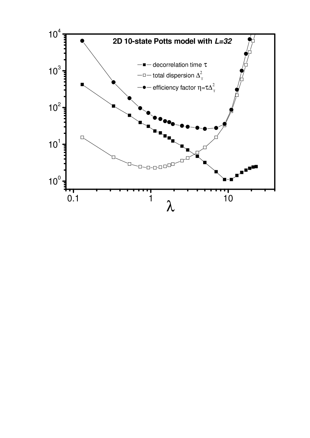
Let us finally reconsider the question about the optimal value of the coupling constant $\lambda$ that allows to achieve the best efficiency by using an extended canonical MC algorithm. An example of such a study is shown in FIG.9, where we illustrate the behavior of the decorrelation time $\tau$ and the total dispersion $\Delta^{2}_{T}=(\Delta E)^{2}/N+N(\Delta\beta_{\omega})^{2}$ for positive values of the coupling constant $\lambda$. The data was obtained from MC simulations of the 2D $10$-state Potts model with $L=32$ by using the extended SW clusters algorithm with environment inverse temperature $\beta_{\omega}(\varepsilon)=\beta_{e}+\lambda(\varepsilon-\varepsilon_{b})$, whose parameters $\beta_{e}=\beta_{c}$ and $\varepsilon_{e}=\varepsilon_{2}$ in order to access the canonically unstable stationary macrostate $\varepsilon_{2}$ located within the anomalous region with $C<0$ at the point of the first-order phase transition $\beta_{c}$.

References

- [1] T. Padmanabhan, Physics Reports 188, 285 (1990).
- [2] D. Lynden-Bell, Physica A 263, 293 (1999).
- [3] D. H. E. Gross, Microcanonical thermodynamics: Phase transitions in Small systems, 66 Lectures Notes in Physics, (World scientific, Singapore 2001).
- [4] D. H. E. Gross and M. E. Madjet, Z. Phys. B 104 (1997) 521.
- [5] L.G. Moretto, R. Ghetti, L. Phair, K. Tso, G.J. Wozniak, Phys. Rep. 287 (1997) 250.
- [6] M. D’Agostino, F. Gulminelli, P. Chomaz, M. Bruno, F. Cannata, R. Bougault, F. Gramegna, I. Iori, N. Le Neindre, GV. Margagliotti, A. Moroni and G. Vannini, Phys. Lett. B 473 (2000) 219.
- [7] P. D. Landau and K. Binder, A guide to Monte Carlo simulations in Statistical Physics (Cambridge Univ Press, 2000).
- [8] L. Velazquez and S. Curilef, J. Phys. A: Math. Theor. 42, 095006 (2009).
- [9] L. Velazquez and S. Curilef, J. Stat. Mech. P03027 (2009).
- [10] N. Metropolis, A. W. Rosenbluth, M. N. Rosenbluth, A. H. Teller and E. Teller, J. Chem. Phys. 21, 1087 (1953).
- [11] W. K. Hastings, Biometrika 57, 97 (1970).
- [12] R.H. Swendsen and J.-S. Wang, Phys. Rev. Lett. 58, 86 (1987).
- [13] J. -S. Wang, R. H. Swendsen and R. Kotecký, Phys. Rev. Lett. 63, 1009 (1989).
- [14] U. Wolff, Phys. Rev. Lett. 62, 361 (1989).
- [15] W. Thirring, Quantum Mechanics of large systems (Springer, 1980) Ch. 2.3.
- [16] J. Viana Lopes et al, Phys. Rev. E 74, 046702 (2006).
- [17] B. Berg and T. Neuhaus, Phys. Lett. B 267, 249 (1991); Phys. Rev. Lett. 68, 9 (1992).
- [18] F. Wang and D. P. Landau, Phys. Rev. Lett. 86, 2050 (2001); Phys. Rev. E 64, 056101 (2001).
- [19] A. Gerling and R. W. Hüller, Z. Phys. B 90, 207 (1993).
- [20] M. S. S. Challa and J. H. Hetherington in Computer Simulation Studies in Condensed Matter Physics I, Eds. D.P. Landau, K. K. Mon and H.-B. Schüttler (Springer, Heidelberg, 1988).
- [21] J. H. Hetherington, J. Low Temp. Phys. 66, 145 (1987).
- [22] R.G. Edwards and A.D. Sokal, Phys. Rev. D 38, 2009 (1988).
- [23] F. Niedermayer, Phys. Rev. Lett. 61, 2026 (1988).
- [24] H.G. Evertz, M. Hasenbusch, M. Marcu, K. Pinn and S. Solomon, Phys. Lett. B 254, 185 (1991).
- [25] M. Hasenbusch, M. Marcu and K. Pinn, Physica A 211, 255 (1994).
- [26] C. Dress and W. Krauth, J. Phys. A 28, L597 (1995).
- [27] J.W. Liu and E. Luijten, Phys. Rev. Lett. 92, 035504 (2004).
- [28] F.Y. Wu, Rev. Mod. Phys. 54, 235 (1982).
- [29] B. A. Berg, in Proceedings of the International Conference on Multiscale Phenomena and Their Simulations, Bielefeld, Oct. 1996, Eds. F. Karsch, B. Monien and H. Satz (World Scientific, Singapore, 1997).
- [30] L. Velazquez and S. Curilef, Equilibrium fluctuation-dissipation relations: A generalization compatible with macrostates with anomalous response functions, Submited to J. Stat. Phys. (2009).