Efficient LLR Calculation for Non-Binary Modulations over Fading Channels
Abstract
Log-likelihood ratio (LLR) computation for non-binary modulations over fading channels is complicated. A measure of LLR accuracy on asymmetric binary channels is introduced to facilitate good LLR approximations for non-binary modulations. Considering piecewise linear LLR approximations, we prove convexity of optimizing the coefficients according to this measure. For the optimized approximate LLRs, we report negligible performance losses compared to true LLRs.
Index Terms:
log-likelihood ratio (LLR), bit-interleaved coded modulation (BICM), Low-density parity-check (LDPC) codes, piecewise linear approximations, fading channelsI Introduction
It is well known that soft-decision decoding algorithms outperform hard-decision decoding algorithms. In soft-decision decoding, reliability metrics are calculated at the receiver based on the channel output. The decoder uses these reliability measures to gain knowledge of the transmitted codewords. The superiority of soft decoding comes at the expense of higher complexity.
Log-likelihood ratios (LLRs) have been shown to be very efficient metrics for soft decoding of many powerful codes such as the convolutional codes [1], turbo codes [2], low-density parity-check (LDPC) codes [3]. LLRs offer practical advantages such as numerical stability and simplification of many decoding algorithms. Moreover, due to some properties of the probability density function (pdf) of the LLRs, such as symmetry and invariance, LLRs are used as convenient tools for the performance analysis of binary linear codes [4, 5, 6]. On many communication channels, even for binary modulations, i.e., binary phase-shift keying (BPSK), channel LLRs are complicated functions of the channel output [7]. This fact greatly increases the complexity of the LLR calculation modules in the decoder causing decoding delays and power dissipation. In high speed wireless transmissions, the decoder may not be able to handle this complexity. Thus, for an efficient implementation of the decoder, approximate LLRs should be considered.
Approximate LLRs have been previously used in the literature [7, 8, 9, 10]. Piecewise linear LLRs have been suggested in [9] for soft Viterbi decoding of convolutional codes in the HIPERLAN/2 standard [11]. The presented method uses the log-sum approximation which is quite accurate at high signal-to-noise ratio (SNR). Moreover, it assumes that perfect channel state information (CSI) is available at the receiver. In [12], linear LLRs have been used for BPSK modulation on uncorrelated fading channels without CSI and a measure of LLR accuracy has been introduced. Using that measure, linear LLR approximating functions have been designed with almost no performance gap to that of true LLR calculation. The proposed measure, however, is only applicable to symmetric channels and BPSK. With non-binary modulations, used in most practical systems, a linear approximation of bit LLRs is not always possible. Moreover, the equivalent bit-channels are asymmetric. That is, the LLR accuracy measure of [12] is not applicable.
In this work, we seek approximate LLRs for non-binary signalling over uncorrelated fading channels. Thus, we need to generalize the accuracy measure of [12] to asymmetric channels. Moreover, we must consider non-linear LLR approximating functions. To compute LLRs at bit levels individually, we consider bit-interleaved coded modulation (BICM) [13]. BICM is a well-known bandwidth efficient scheme for binary codes on fading channels.
While our approaches are general, to demonstrate our methods, we focus on piecewise linear approximations. Such approximations are easy to implement and we observe that, when the parameters are optimized, they perform close to true LLRs. We prove that the optimization of these piecewise linear approximations is convex, thus, very efficient. Due to the close-to-capacity performance of LDPC codes on many channels [14, 15, 8], we employ LDPC-coded BICM [16] to show that even with the proposed approximation, close-to-capacity performance is obtained.
II Problem Definition
Consider a flat slow-fading environment where the received signal is expressed as
where is the complex transmitted signal chosen from the signal set of size , is the channel fading gain with arbitrary pdf , and is the additive noise which is a complex zero-mean white Gaussian random variable with variance .
II-A LLRs for equivalent bit-channels
Using the BICM scheme [13], the information sequence is first encoded by a binary code. Next, the coded sequence is bit interleaved and is broken into -bit sequences which are then Gray labeled onto signals in and transmitted on the channel. Assuming ideal interleaving, the system can be seen equivalently as parallel independent and memoryless binary-input bit-channels. In the receiver, based on , LLRs are computed for each bit-channel independently from other bits. These LLRs are then de-interleaved and passed to the decoder.
When the channel fading gain is known at the receiver for each channel use, the true LLR for the th bit-channel, assuming uniform input distribution, is calculated as
| (1) |
where , is the th bit of the label of , is the subset of signals in where , and the conditional distributions are given by or when the signal set is real. Also, represents as a function of when is known. When is not known at the receiver, the true LLR is calculated as
| (2) |
where , and represents as a function of .
As can be seen from (1) and (2), both and are usually complicated functions of . Thus, approximate LLRs ( and ) are of practical interest. One approximation which is useful at high SNR is obtained by the log-sum approximation: . This approximation is good when the sum is dominated by a single large term. Thus,
| (3) |
The log-sum approximation is particularly useful when CSI is available at the receiver, where (3) leads to piecewise linear LLRs which can be efficiently implemented [9]. However, with no CSI, the log-sum approximation is no longer piecewise linear and in fact involves complicated integrations. The focus of our work is on cases that CSI is not available. Nonetheless, we seek approximate LLRs which are piecewise linear functions of
Now, consider a general LLR approximation function parameterized by set of parameters
This function maps the complex received signal to real-valued approximate LLR for the th bit-channel. Clearly, it is desired to choose such that accurate LLR estimates are obtained. To this end, we first extend the LLR accuracy measure introduced in [12] to non-symmetric bit-channels obtained via BICM. We then use this measure for optimizing the LLR approximating functions.
II-B LLR accuracy measure for asymmetric binary-input channels
In this section, we generalize the LLR accuracy measure of [12] to asymmetric channels. To this end, we consider the pdfs of the th bit-channel LLR conditioned on the transmitted bit defined as Using these LLR pdfs, it is possible to calculate the capacity of each asymmetric bit-channel and thus the BICM scheme. By capacity, we mean the mutual information between the input and output of each bit-channel when its input is equally likely or . The capacity of the th bit-channel is given by [17]
| (4) |
Thus, the capacity of the BICM is found by
When instead of the true LLRs, approximate LLRs are used, their pdfs are given by for . Inserting these approximate LLR pdfs in (4) we get
| (5) |
The following theorem, proved in Appendix A, shows can be used as an LLR accuracy measure.
Theorem 1.
The maximum of in (5) is equal to which is achieved by true LLRs (no LLR approximation can result in ).
Notice that for a symmetric channel (i.e., ), (5) reduces to the LLR accuracy measure of [12]. Using similar arguments, it can be shown that as the approximate LLRs drift away more from the true LLRs, gets larger. Thus, is a measure of the accuracy of the approximate bit LLRs. Since bit-channels are independent, we maximize each individually. Thus, for each bit-channel , assuming a class of approximating functions , we find:
| (6) | |||||
where denotes the constraints imposed on (e.g., to preserve continuity).
II-C LLR approximating functions
It is evident from (1) and (2) that true LLR functions depend on the signal set . Thus, choosing appropriate class of approximating functions also depends on . In this letter, we consider non-binary AM and rectangular QAM. Our optimization approach, however, is general. Moreover, we put our focus on piecewise linear approximate LLRs. Clearly, the optimization problem (6) can be solved for any other approximating function. Using piecewise linear approximations has benefits such as simplicity of demodulator and (as will be shown) convexity of the optimization problem. Numerical results verify that the obtained performance is also very close to true LLRs.
By viewing a complex variable as a two-dimensional vector , a piecewise linear function of a complex variable is defined as follows. First, the complex domain is divided into a finite number of regions by a finite number of one-dimensional boundaries. Then the function is represented by for any , where denotes the inner product of two-dimensional vectors, i.e., . Thus,
| (7) |
where is the number of segments of the piecewise linear function, is the set of all , , and is the indicator function. The parameters are chosen to preserve continuity over .
The following theorem, proved in Appendix B, indicates that optimizing a piecewise linear approximating function according to (6) is a convex optimization problem.
Theorem 2.
Assuming that approximate bit LLRs are calculated by (7) for , and assuming fixed for , is a concave function of and for all
Using (7), (6) can be numerically solved as follows. For a given SNR, and assuming fixed ’s, can be computed by first computing and for given ’s and ’s and inserting them in (5). Since is a concave function of ’s and ’s and the constraints are linear, maximizing can be done efficiently using numerical optimization techniques. The proper number of regions is based on the affordable complexity and the curve of true LLRs. Optimizing the regions can be done through search. As will be seen in the next section, usually the size of the parameter sets is small and due to the symmetry in the LLR calculation, many parameters are equal to each other which can further reduce the number of unknown parameters.
III Proposed Approach and Examples
Now, we describe the proposed method through examples of real and complex signal constellations.
Example 1: Consider 8-AM constellation with Gray labeling shown in Fig. 1 on the normalized Rician fading channel. On this channel, , where is the Rician K-factor, and is the zero-order modified Bessel function of the first kind.
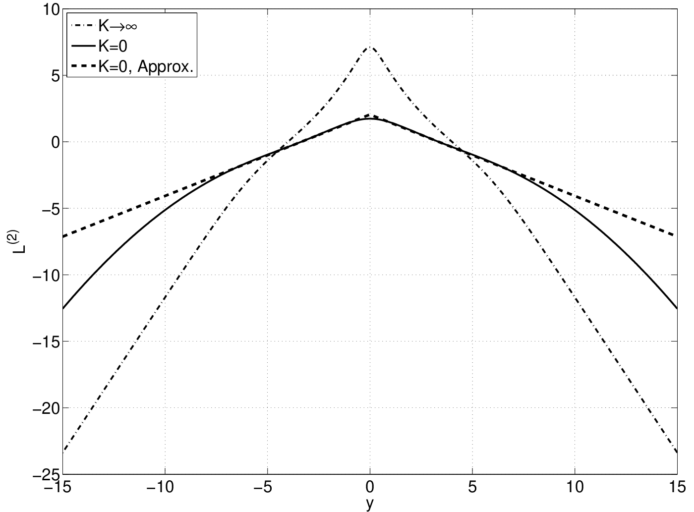
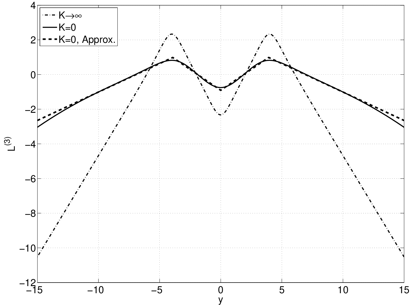
Using (1) and (2), true LLRs are calculated for , and they have been plotted versus for extreme values of in Fig. 2. Considering the general model of (7), and the symmetry in the true LLR functions, we propose the following piecewise linear LLR approximations
| (8) | |||||
| (9) | |||||
| (10) | |||||
where due to the symmetry of the LLRs, we have assumed in (9) that and . Also, in (10), we have , , , , and . Thus, , , and . It is evident that symmetry reduces the number of unknown parameters. We also impose to preserve continuity in (10). Fig. 2 shows that these piecewise linear functions better approximate the true LLRs when increases.
For a given SNR, we optimize the parameter sets , , and , by solving (6). Numerical results confirm that is always very close to the capacity of BICM employing true LLRs, i.e., . For example, for , and bits per channel use at SNR dB, and and bits per channel use at SNR dB. When increases, becomes even smaller.
To evaluate the decoding performance of the optimized piecewise linear approximations, we compare the decoding threshold of LDPC codes and their bit error rate (BER) under approximate and true LLRs. The decoding threshold can be found by density evolution [5, 14] and by using the technique of i.i.d. channel adapters [16] which provides the required symmetry conditions.
As an example, consider -regular LDPC codes on the normalized Rayleigh channel (equivalent to ) with 8-AM signalling of Fig. 1. By using the approximating functions of (8)–(10), we find the decoding threshold of the code under optimized LLR parameters reported in Table I. The decoding threshold given by density evolution is 7.88 dB while under true LLR calculation of (2), the decoding threshold is 7.85 dB showing only a 0.03 dB performance gap.
To see how the piecewise linear LLR calculation affects the BER performance, we simulate a given LDPC code on the normalized Rayleigh fading channel. In Fig. 3, the performance of a randomly constructed -regular LDPC code of length is depicted in two cases: once decoded using true LLRs of (2), and once with the piecewise linear approximation of (8)–(10) and the optimized parameters reported in Table I. It should be noted that the parameters are optimized once at the decoding threshold and are kept fixed at the receiver for other SNRs. It is seen that the performance of the optimized approximate LLRs is almost identical to that of the more complex true LLRs although parameters are only optimized for the worst SNR.
Also, to show that optimizing is meaningful in terms of the maximum transmission rate achievable by the piecewise linear LLRs, we optimize the degree distributions [18] of LDPC codes under our approximate LLRs. At SNR dB, the capacity of BICM under true LLRs is in the absence of CSI when . Since , then the maximum binary code rate achievable on this channel is . At this SNR, solving (6) gives and the parameters reported in Table I. Now, by using the designed piecewise linear approximation, assuming a fixed check node degree of and maximum variable node degree of , an irregular LDPC code is designed. The variable node degree distribution of this code is , and the code rate is . Thus, the proposed approximate LLRs can achieve rates very close to the capacity of BICM under true LLRs.
Example 2: Now consider a 16-QAM constellation with Gray labeling as depicted in Fig. 1. Using the general piecewise linear model of (7), due to the symmetry and the similarity of the bit LLR functions, we propose the following LLR approximations:
| (11) | |||||
| (12) | |||||
where are the four quadrants of the complex plane. It should be noted that bit-channel LLR calculations are similar for bit 1 and 3, and for bit 2 and 4 except that the real and imaginary parts of are swapped, i.e., and . Thus, it is enough to optimize and .
Again numerical results suggest that the gap between and the true BICM capacity is always small. For example, when , we have and bits per channel use at SNR= dB. Again, the gap becomes smaller when increases.
To investigate the performance of 16-QAM signalling under the proposed approximate LLRs, we compare the decoding threshold and BER of -regular LDPC codes on the Rayleigh fading channel under true and approximate LLRs. Density evolution gives a decoding threshold of dB under approximate LLRs with the optimized parameters of Table I. Under true LLR calculation, the decoding threshold is dB. As a result, approximate LLRs show about dB performance gap to true LLRs. The BER comparison is depicted in Fig. 3. It is worth mentioning that this gap can be further reduced by proposing piecewise linear LLRs with more segments.
IV Conclusion
LLR computation for equivalent bit-channels of a non-binary modulation is generally complicated. On fading channels, when the channel gain is unknown, this problem is further intensified. Noticing that the equivalent bit channels were asymmetric, in order to find good approximate LLRs, we proposed an LLR accuracy measure for binary asymmetric channels. This accuracy measure can be used to optimize the parameters of any approximating function. We used our accuracy measure to optimize piecewise linear LLR approximations. By using LDPC-coded BICM, we showed that the performance loss under the optimized piecewise linear approximation was very small. We also showed that under approximate LLRs, asymptotic irregular LDPC codes having rates very close to the capacity of BICM under true LLRs can be obtained. Our solution can also be applied to other coding schemes which use LLRs such as the convolutional and turbo codes.
Appendix A Proof of Theorem 1
Consider an arbitrary discrete binary-input memoryless channel whose output alphabet is non-binary. The channel input is , and its output is . Let us define and where . The true LLR value, when is observed at the channel output and the binary inputs are equiprobable, is
| (13) |
Thus, the true LLR pdf when is sent is given by and by when is sent over the channel.
Now, assuming that when is observed at the channel output, the approximate LLR is calculated by , the conditional pdfs of are:
| (14) | |||||
| (15) |
Inserting (14) and (15) in (4) gives
| (16) |
Taking reveals that maximizes for all since for all and for all and and . These values of ’s are equal to the true LLR of (13). Thus, the maximizing point is only given by true LLRs. Noticing that these results are valid for each equivalent bit-channel of the BICM and since in (5), the theorem is proved.
Appendix B Proof of Theorem 2
Denote and for . Then can be written as
By using (7) and with some abuse of notation we write
For each fixed , it is clear that is a linear function of and . Noticing that the function is convex and twice differentiable, it can be deduced that is also a convex function of and . The convexity is also preserved under expectation. Thus, is also convex which makes concave with respect to and for all .
References
- [1] S. Lin and D. J. Costello, Error Control Coding, Second Edition. Upper Saddle River, NJ, USA: Prentice-Hall, Inc., 2004.
- [2] C. Berrou, A. Glavieux, and P. Thitimajshima, “Near Shannon limit error-correcting coding and decoding: Turbo-codes (1),” in Conf. Rec. IEEE ICC ’93, vol. 2, Geneva, Switzerland, May 1993, pp. 1064–1070.
- [3] R. G. Gallager, “Low-Density Parity-Check codes,” Ph.D. dissertation, MIT press, Cambridge, MA, 1963.
- [4] I. Land, P. A. Hoeher, and U. Sorger, “Log-likelihood values and Monte Carlo simulation: some fundamental results,” in Proc. Int. Symp. on Turbo Codes and Related Topics, Brest, France, Sept 2000.
- [5] T. J. Richardson, M. A. Shokrollahi, and R. L. Urbanke, “Design of capacity-approaching irregular low-density parity-check codes,” IEEE Trans. Inf. Theory, vol. 47, no. 2, pp. 619–637, Feb. 2001.
- [6] A. Abedi and A. K. Khandani, “Invariance properties of binary linear codes over a memoryless channel with discrete input,” IEEE Trans. Inf. Theory, vol. 53, no. 3, pp. 1215–1218, Mar 2007.
- [7] J. Hagenauer, “Viterbi decoding of convolutional codes for fading- and burst-channels,” in Zurich seminar on digital communications, 1980.
- [8] J. Hou, P. H. Siegel, and L. B. Milstein, “Performance analysis and code optimization of low-density parity-check codes on Rayleigh fading channels,” IEEE J. Sel. Areas Commun., vol. 19, no. 5, pp. 924–934, May 2001.
- [9] F. Tosato and P. Bisaglia, “Simplified soft-output demapper for binary interleaved COFDM with application to HIPERLAN/2,” in Proc. of the 2002 IEEE International Conference on Communications (ICC’02), 2002, pp. 664–668.
- [10] J. K. Kwon, S. Park, and D. K. Sung, “Log-likelihood ratio (LLR) conversion schemes in orthogonal code hopping multiplexing,” IEEE Commun. Lett., vol. 7, no. 3, pp. 104–106, Mar. 2003.
- [11] ETSI TS 101 475, “Broadband Radio Access Networks (BRAN); HIPERLAN Type 2; Physical (PHY) layer, v1.2.2,” 2001.
- [12] R. Yazdani and M. Ardakani, “Linear LLR approximation for iterative decoding on wireless channels,” IEEE Trans. Commun., vol. 57, no. 11, pp. 3278–3287, Nov. 2009.
- [13] G. Caire, G. Taricco, and E. Biglieri, “Bit-interleaved coded modulation.” IEEE Trans. Inf. Theory, vol. 44, no. 3, pp. 927–946, 1998.
- [14] S.-Y. Chung, G. D. Forney, T. J. Richardson, and R. Urbanke, “On the design of low-density perity-check codes within 0.0045 dB of the Shannon limit,” IEEE Commun. Lett., vol. 5, no. 2, pp. 58–60, Feb. 2001.
- [15] M. Luby, M. Mitzenmacher, A. Shokrollahi, and D. Spielman, “Efficient erasure correcting codes,” IEEE Trans. Inf. Theory, vol. 47, pp. 569–584, 2001.
- [16] J. Hou, P. H. Siegel, L. B. Milstein, and H. D. Pfister, “Capacity-approaching bandwidth-efficient coded modulation schemes based on low-density parity-check codes,” IEEE Trans. Inf. Theory, vol. 49, no. 9, pp. 2141–2155, Sept. 2003.
- [17] A. Sanaei and M. Ardakani, “LDPC code design considerations for non-uniform channels,” IEEE Trans. Commun., Jan. 2010.
- [18] M. G. Luby, M. Mitzenmacher, M. A. Shokrollahi, and D. A. Spielman, “Improved low-density parity-check codes using irregular graphs,” IEEE Trans. Inf. Theory, vol. 47, no. 2, pp. 585–598, Feb. 2001.
| 8-AM | ||||||||
| SNR | Bit 1 | Bit 2 | Bit 3 | |||||
| 7.88 dB | ||||||||
| 21.03 dB | ||||||||
| 16-QAM | ||||||||
| SNR | Bit 1 | Bit 2 | ||||||
| 5.02 dB | ||||||||