1Introduction

August 24, 2026

TUM-HEP-750/10

Patterns of Flavour Violation in the Presence of
a Fourth Generation of Quarks and Leptons

Andrzej J. Buras^a,b, Björn Duling^a, Thorsten Feldmann^a,

Tillmann Heidsieck^a, Christoph Promberger^a, Stefan Recksiegel^a

^aPhysik Department, Technische Universität München, James-Franck-Straße,
D-85748 Garching, Germany

^bTUM Institute for Advanced Study, Technische Universität München, Arcisstr. 21,
D-80333 München, Germany

We calculate a number of observables related to particle-antiparticle mixing and the branching ratios for the most interesting rare and CP-violating $K$ and $B$ decays in the Standard Model (SM3) extended by a fourth generation of quarks and leptons (SM4). A model-independent parametrisation of these observables in terms of gauge-independent functions is adopted, which is useful for studying the breaking of the universality between $K$ , $B_{d}$ and $B_{s}$ systems through non-minimal flavour violating interactions. We calculate first the mass differences $\Delta M_{i}$ in the neutral $K$ and $B$ systems, the mixing-induced CP asymmetries $S_{\psi K_{S}}$ , $S_{\psi\phi}$ , $S_{\phi K_{S}}$ , $S_{\eta^{\prime}K_{S}}$ and $\varepsilon_{K}$ . Subsequently, a detailed analysis of $K^{+}\to\pi^{+}\nu\bar{\nu}$ , $K_{L}\to\pi^{0}\nu\bar{\nu}$ , $B_{s,d}\to\mu^{+}\mu^{-}$ , $B\to X_{s,d}\nu\bar{\nu}$ , $K_{L}\to\pi^{0}\ell^{+}\ell^{-}$ , $B\to X_{s}\gamma$ and $B\to X_{s,d}\ell^{+}\ell^{-}$ is presented, and also $\varepsilon^{\prime}/\varepsilon$ is considered. For some of these observables the departures from SM3 predictions can still be spectacular.

We discuss how the new mixing parameters (3 angles, 2 CP phases) can be determined using the flavour observables in question. We identify the different hierarchical structures in the SM4 flavour mixing matrix, allowed by phenomenological and theoretical constraints, and define the corresponding generalised Wolfenstein expansion. Most importantly, we show how the characteristic patterns of correlations among the considered flavour observables allow to distinguish this New Physics scenario from supersymmetric flavour models, the Littlest Higgs model with T-parity and the Randall-Sundrum model with custodial protection. Of particular importance are the correlations involving $S_{\psi\phi}$ , $S_{\phi K_{S}}$ , ${\rm Br}(K^{+}\rightarrow\pi^{+}\nu\bar{\nu})$ , ${\rm Br}(K_{L}\rightarrow\pi^{0}\nu\bar{\nu})$ and ${\rm Br}(B_{s,d}\rightarrow\mu^{+}\mu^{-})$ , which could in principle rule out the SM4. Interestingly $\varepsilon^{\prime}/\varepsilon$ turns out to be suppressed below the data for large positive values of $S_{\psi\phi}$ unless the relevant hadronic matrix elements differ strongly from the large $N$ results. The important role of $\varepsilon^{\prime}/\varepsilon$ in bounding large enhancements of rare $K$ decay branching ratios is reemphasised. We also show how the existing anomalies in the unitarity triangle fits as well as in $S_{\psi\phi}$ and $S_{\phi K_{S}}$ can be simultaneously explained in the SM4 scenario.

1 Introduction

One of the simplest extensions of the Standard Model (hereafter referred to as SM3) is the addition of a sequential fourth generation (4G) of quarks and leptons [1] (hereafter referred to as SM4). While the setup we are considdering here (e.g. perturbative Yukawa couplings) does not address any of the known hierarchy and naturalness problems, if present in nature, a 4G is likely to have a number of profound implications that makes it interesting to consider. These are:

1.

While being consistent with electroweak precision data (EWPT) [2, 3, 4, 5, 6, 7], a 4G can remove the tension between the SM3 fit and the lower bound on the Higgs mass $m_{H}$ from LEP II. Indeed, as pointed out in [3, 5, 8], a heavy Higgs boson does not contradict EWPT as soon as the 4G exists.
2.

$SU(5)$ gauge coupling unification could in principle be achieved without supersymmetry [9], although the present lower bound on the masses of 4G quarks and the appearance of Landau poles in Yukawa couplings well below the GUT scales practically excludes this possibility if one wants to stay within a perturbative framework at short-distance (SD) scales.
3.

Electroweak baryogenesis might be viable [10, 11, 12].
4.

Most importantly, from the point of view of the present paper, certain anomalies present in flavour-changing processes could in principle be resolved [13, 14, 15].
5.

The structure of the lepton sector in the SM4 can be interesting as shown recently in [16]: a heavy (mostly Dirac) 4G neutrino in addition to very light (mostly Majorana) neutrinos can be obtained in a setup with electroweak symmetry breaking in warped extra dimensions.

On the other hand there are scenarios where a fourth generation might trigger dynamical breaking of electroweak symmetry [17, 18, 19, 20, 21, 22, 23]. However since it is in the very nature of non-perturbative Yukawa couplings to defy direct calculations there is until now no explicit model for this scenario.

There is a rich literature on the implications and phenomenology of the SM4. Reviews and summary statements can be found in [1, 24]. In particular during the last years, a number of analyses were published with the goal to investigate the impact of the existence of a 4G on Higgs physics [5], electroweak precision tests [4, 5, 6, 7] and flavour physics [25, 13, 14, 15, 26, 27, 28]. In this context, Bobrowski et al. [27] have studied the constraint on the mixing between the fourth and third generation by using FCNC processes, and Chanowitz [6] by using global fits to EWPT. Interesting bounds on this mixing could be derived in this manner. We will address these bounds in the course of our analysis.

Detailed analyses of supersymmetry in the presence of a 4G have recently been performed in [29, 30]. These analyses show that the marriage of SUSY with the SM4 is rather challenging because of Landau poles in Yukawa couplings present at relatively low scales. The last paper contains a good up to date collection of references to papers on the SM4.

In the present paper we will take a different strategy by considering, in addition to $\Delta F=2$ transitions and $B\to X_{s}\gamma$ and $B\to X_{s}\ell^{+}\ell^{-}$ decays as done in [15, 27], also rare $K$ and $B$ decays, as considered in [13], on which new data will be available in the coming decade. In particular,

i)

We will establish a number of correlations between various observables that should allow us to distinguish this NP scenario from the Littlest Higgs model with T-parity (LHT), the Randall-Sundrum model with custodial protection (RSc) and supersymmetric flavour models that have been analysed in [31, 32, 33, 34, 35, 36] recently. We will also carefully study how these correlations depend on the size of the 4G mixing angles and phases.
ii)

For the most interesting observables, we will investigate the departures from models with (constrained) minimal flavour violation ((C)MFV), taking into account all existing constraints.
iii)

We will demonstrate transparently how certain anomalies observed in the unitarity triangle fits and in the CP asymmetries $S_{\psi\phi}$ and $S_{\phi K_{S}}$ can be resolved simultaneously and how these solutions affect other observables.
iv)

We will address the question how the additional five parameters of the $4\times 4$ quark mixing matrix, $\theta_{14}$ , $\theta_{24}$ , $\theta_{34}$ , $\delta_{14}$ and $\delta_{24}$ , could — in principle — be determined by means of the mixing-induced CP asymmetries $S_{\psi\phi}$ and $S_{\psi K_{S}}$ , the $B^{0}_{d,s}-\bar{B}_{d,s}$ mixing mass differences $\Delta M_{d,s}$ , $\epsilon_{K}$ and the branching ratios for the rare decays $K^{+}\to\pi^{+}\nu\bar{\nu}$ , $K_{L}\to\pi^{0}\nu\bar{\nu}$ , $B_{s,d}\to\mu^{+}\mu^{-}$ , $B\to X_{s}\nu\bar{\nu}$ .
v)

On the theoretical side, we will discuss how the SM4 can be understood as a particular realisation of a next-to-minimal flavour violation scenario. This introduces certain consistency conditions between the SM3 and SM4 mixing angles which can be used to eliminate “fine-tuned” values in parameter space. The remaining cases can be classified according to the scaling of the 4G mixing angles with the Cabibbo angle, and for each individual case an SM4 generalisation of the Wolfenstein parametrisation can be constructed.

Our paper is organised as follows: In Section 2, we discuss the flavour symmetries in the SM4, provide the $4\times 4$ quark mixing matrix and address the question of possible hierarchies between the 4G mixing angles. In Section 3, we generalise the effective weak Hamiltonians to the SM4. In Section 4, we compile basic formulae for FCNC processes considered in our paper. As the SM4 goes beyond MFV, but the operator structure of the SM3 effective Hamiltonian remains intact, it is very efficient to introduce – as done in the LHT model [31, 32, 33] – generalised complex master functions $S_{i},\,X_{i},\,Y_{i},\,Z_{i},\,D_{i}^{\prime},\,E_{i}^{\prime},\,E_{i},\,(i=K,d,s)$ , that enter the expressions for various observables. On the one hand, in the absence of the 4G, these functions reduce to the SM3 flavour-universal functions $S_{0}$ , $X_{0}$ , $Y_{0}$ , $Z_{0}$ , $D^{\prime}_{0}$ , $E^{\prime}_{0}$ and $E_{0}$ . On the other hand, using these functions, non-MFV effects in this model can be very transparently compared to those found in the LHT model.

In Section 5, we summarise the insights gained by other authors, who studied in particular the impact of the 4G on the electroweak precision observables. In Section 6, we will summarise our strategy for the phenomenological analysis of the SM4. In Section 7, we present a detailed global numerical analysis, using the formulae of previous sections. In particular, we identify a number of correlations between various observables, and we estimate approximate upper bounds on several CP asymmetries and branching ratios. In Section 8, we study the anatomy of flavour effects in the SM4 scenario. In this context, we address the most important phenomenological anomalies found in the present flavour data.

In Section 9, we outline an efficient procedure how to constrain the new mixing angles $\theta_{14}$ , $\theta_{24}$ , $\theta_{34}$ and the new phases $\delta_{14}$ and $\delta_{24}$ from

	$\displaystyle S_{\psi\phi}\,,\quad S_{\psi K_{S}}\,,\quad\Delta M_{d,s}\,,\quad\epsilon_{K}\,,$		(1.1)
	$\displaystyle{\rm Br}(K^{+}\to\pi^{+}\nu\bar{\nu})\,,\ \,{\rm Br}(K_{L}\to\pi^{0}\nu\bar{\nu})\,,\ \,{\rm Br}(B_{s,d}\to\mu^{+}\mu^{-})\,,\ \,{\rm Br}(B\to X_{s,d}\nu\bar{\nu})\,.$		(1.2)

For this purpose, we will provide a classification of the 4G mixing parameters which allows us to connect the different patterns found in flavour observables to particular properties of the 4G mixing angles and CP phases. Finally, in Section 10, we summarise our main findings. Here we will also compare the patterns of flavour violation in the SM4 with those found in supersymmetric flavour models, the LHT model and the RSc model. An appendix collects the one-loop functions used in our paper.

2 The $4\times 4$ Mixing Matrix $V_{\text{SM4}}$

2.1 Yukawa Couplings and (Approximate) Flavour Symmetries

The SM4 quark Yukawa sector involves two $4\times 4$ Yukawa matrices,

-{\cal L}_{\rm Yuk}=\bar{Q}_{L}\,Y_{U}^{\rm SM4}\,\tilde{H}\,U_{R}+\bar{Q}_{L}\,Y_{D}^{\rm SM4}\,H\,D_{R}+\mbox{h.c.}\,.

(2.1)

Following [37], we identify the Yukawa couplings as spurions, being the (only) sources for the breaking of the flavour symmetry in the SM4,

\displaystyle G_{F}^{\rm SM4}

\displaystyle=SU(4)_{Q_{L}}\times SU(4)_{U_{R}}\times SU(4)_{D_{R}}\times U(1)_{U_{R}}\times U(1)_{D_{R}}\,,

(2.2)

where we have divided out one $U(1)$ factor corresponding to the conserved baryon number. Under the flavour symmetry, the Yukawa spurions transform as

\displaystyle Y_{U}^{\rm SM4}\sim(4,\bar{4},1)_{1,0}\,,\hskip 22.99988ptY_{D}^{\rm SM4}\sim(4,1,\bar{4})_{0,1}\,.

(2.3)

As in the SM3 case (see also [38, 39, 40]), the counting of symmetry generators (related to 18 angles + 29 phases) vs. complex Yukawa entries (32 + 32) gives the number of physical parameters

14+3=\mbox{8 masses}+\mbox{6 angles}+\mbox{3 phases}\,,

i.e. 2 additional masses, 3 additional angles and 2 additional phases compared to the SM3 case.

Alternatively, we can consider the flavour symmetries from the SM3 point of view: Taking only the large $t^{\prime}$ and $b^{\prime}$ Yukawa couplings into account, the effective flavour symmetry is

\displaystyle G_{\rm eff}^{\rm SM3}

\displaystyle=SU(3)_{Q_{L}}\times SU(3)_{U_{R}}\times SU(3)_{D_{R}}\times U(1)_{U_{R}}\times U(1)_{D_{R}}\times U(1)_{Q^{\prime}}\,,

(2.4)

which, compared to the SM3 case, involves an additional $U(1)_{Q^{\prime}}$ symmetry, since – without mixings involving the first three generations – the 4G quark number is approximately conserved. The mixings between the fourth and the first three generations can be parametrised by an $SU(3)_{Q_{L}}$ triplet which is charged under the $U(1)_{Q^{\prime}}$ ,

\displaystyle\chi_{L}\sim(3,1,1)_{0,0,1}\,.

(2.5)

Of the six independent entries of $\chi_{L}$ , one phase is unobservable due to the $U(1)_{Q^{\prime}}$ symmetry, leaving exactly the additional 3 mixing angles and 2 CP-violating phases of the SM4. The remaining parameters for the first three generations are contained in SM3 Yukawa matrices

\displaystyle Y_{U}^{\rm SM3}\sim(3,\bar{3},1)_{1,0,0}\,,\hskip 22.99988ptY_{D}^{\rm SM3}\sim(3,1,\bar{3})_{0,1,0}\,.

(2.6)

The so-defined SM4 thus provides a particular example of the next-to-minimal flavour violating construction discussed in [41], with new non-minimal flavour structures generated by means of the $\chi_{L}$ spurion. Using a non-linear parametrisation (as it has been used for the SM3 case in [42, 43]),

\displaystyle Y_{U}^{\rm SM4}

\displaystyle=\xi_{L}^{\dagger}\left(\begin{array}[]{cc}Y_{U}^{\rm SM3}&\begin{array}[]{c}0\\ 0\\ 0\end{array}\\ \begin{array}[]{ccc}0&0&0\end{array}&y_{t^{\prime}}\end{array}\right)\,,\hskip 22.99988ptY_{D}^{\rm SM4}=\xi_{L}\,\left(\begin{array}[]{cc}Y_{D}^{\rm SM3}&\begin{array}[]{c}0\\ 0\\ 0\end{array}\\ \begin{array}[]{ccc}0&0&0\end{array}&y_{b^{\prime}}\end{array}\right)\,,

we introduce the $4\times 4$ matrix

\displaystyle\xi_{L}

\displaystyle=\exp\left[i\left(\begin{array}[]{cc}\begin{array}[]{ccc}0&0&0\\ 0&0&0\\ 0&0&0\end{array}&\chi_{L}\\ \chi_{L}^{\dagger}&0\end{array}\right)\right]\,.

It transforms as $V_{Q_{L}}\xi_{L}V_{Q_{L}}^{\dagger}$ where $V_{Q_{L}}$ contains an $SU(3)_{Q_{L}}$ block matrix for the SM3 generations, while the 4G fields remain constant. The consistency conditions discussed in [41] translate into

		$\displaystyle\|(\chi_{L})_{i}\|\|(\chi_{L})_{j}\|\ \lesssim\ \theta_{ij}\,,\hskip 22.99988pt$		$\displaystyle(i,j=1\ldots 3)$		(2.19)
	$\displaystyle\Leftrightarrow\hskip 22.99988pt$	$\displaystyle\theta_{ik}\theta_{jk}\ \lesssim\ \theta_{ij}\hskip 22.99988pt$		$\displaystyle(i,j,k=1\ldots 4)$		(2.20)

where no summation over ”k” is understood. Here $\theta_{12}\sim\lambda$ , $\theta_{23}\sim\lambda^{2}$ , $\theta_{13}\sim\lambda^{3}$ are the SM3 mixing angles and $\theta_{i4}$ the 4G mixing angles (see below). Notice that for the SM3 case, one has one of the inequalities (2.20) saturated,

\displaystyle\theta_{12}\theta_{23}\sim\theta_{13}\,,\hskip 22.99988pt\mbox{but}\hskip 22.99988pt\theta_{12}\theta_{13}\ll\theta_{23}\,,\hskip 11.49994pt\theta_{13}\theta_{23}\ll\theta_{12}\,.

(2.21)

A particular way to realise the constraints (2.20) is to consider a simple Froggatt-Nielsen (FN) setup [44], where the scaling of the mixing angles is controlled by different $U(1)$ charge factors $b_{i}$ for the left-handed doublets of different generations, leading to

\displaystyle\theta_{ij}\sim\lambda^{|b_{i}-b_{j}|}\,.

(2.22)

Here $\lambda$ is given by the VEV of some $U(1)$ -breaking scalar field divided by a large UV-scale. The triangle inequalities for $|b_{i}-b_{k}|+|b_{k}-b_{j}|$ then guarantee that (2.20) always holds. Since (2.22) only involves charge differences, we may set $b_{4}\equiv 0$ , while the charges $b_{1-3}$ and the related 4G mixing angles are not completely fixed. However, we can identify certain benchmark cases which may later be compared with the phenomenological constraints from EWPT, tree-level decays and rare decays of SM3 quarks: Scenarios with some 4G mixing angles being of order ${\cal O}(1)$ are already ruled out by EWPT [4, 6] and tree-level quark decays (see below). Among the interesting scenarios with sufficiently small mixing angles, we identify:

(a)

b_{3}=1

b_{2}=3

b_{1}=4

\displaystyle\hskip 11.49994pt\Rightarrow\hskip 11.49994ptV_{\text{SM4}}\sim\left(\begin{array}[]{cccc}1&\lambda&\lambda^{3}&\lambda^{4}\\ \lambda&1&\lambda^{2}&\lambda^{3}\\ \lambda^{3}&\lambda^{2}&1&\lambda\\ \lambda^{4}&\lambda^{3}&\lambda&1\end{array}\right)\,,

which yields a very symmetric scaling pattern for the 4G mixing matrix, and shares the feature of the SM3 CKM matrix that more off-diagonal elements get smaller. Notice that of the 9 inequalities in (2.20) involving the 4G mixing angles, 3 are saturated, namely

(a)

\displaystyle\hskip 11.49994pt\theta_{12}\theta_{24}\sim\theta_{13}\theta_{34}\sim\theta_{14}\,,\hskip 11.49994pt\theta_{24}\sim\theta_{23}\theta_{34}\,.

(2.27)

Scenarios with even smaller mixing angles ( $\theta_{i4}\to\lambda^{n}\theta_{i4}$ ) can simply be obtained from (2.1) by increasing $b_{1-3}\to b_{1-3}+n$ . An FN example for a scenario with (relatively) large 4G mixing angles is given by

(b)

b_{3}=1

b_{2}=-1

b_{1}=-2

\displaystyle\hskip 11.49994pt\Rightarrow\hskip 11.49994ptV_{\text{SM4}}\sim\left(\begin{array}[]{cccc}1&\lambda&\lambda^{3}&\lambda^{2}\\ \lambda&1&\lambda^{2}&\lambda\\ \lambda^{3}&\lambda^{2}&1&\lambda\\ \lambda^{2}&\lambda&\lambda&1\end{array}\right)\,,

In this case, the saturated inequalities are

(b)

\displaystyle\hskip 11.49994pt\theta_{14}\theta_{34}\sim\theta_{13}\,,\hskip 11.49994pt\theta_{24}\theta_{34}\sim\theta_{23}\,,\hskip 11.49994pt\theta_{12}\theta_{24}\sim\theta_{14}\,.

(2.32)

For later use, we further identify two interesting non-FN scenarios. The first one is given by

(c)

\displaystyle\hskip 11.49994ptV_{\text{SM4}}\sim\left(\begin{array}[]{cccc}1&\lambda&\lambda^{3}&\lambda^{2}\\ \lambda&1&\lambda^{2}&\lambda^{3}\\ \lambda^{3}&\lambda^{2}&1&\lambda\\ \lambda^{2}&\lambda^{3}&\lambda&1\end{array}\right)\hskip 11.49994pt\mbox{with}\ \ \theta_{14}\theta_{34}\sim\theta_{13}\,,\ \theta_{12}\theta_{14}\sim\theta_{23}\theta_{34}\sim\theta_{24}\,.

In this case, the SM4 mixing matrix takes a very symmetric form, where the mixing angle $\theta_{14}$ between the fourth and first generation is larger than $\theta_{24}$ . Finally, for

(d)

\displaystyle\hskip 11.49994ptV_{\text{SM4}}\sim\left(\begin{array}[]{cccc}1&\lambda&\lambda^{3}&\lambda^{3}\\ \lambda&1&\lambda^{2}&\lambda^{2}\\ \lambda^{3}&\lambda^{2}&1&\lambda\\ \lambda^{3}&\lambda^{2}&\lambda&1\end{array}\right)\hskip 22.99988pt\mbox{with}\hskip 11.49994pt\theta_{12}\theta_{24}\sim\theta_{14}\,

we encounter the situation that the mixing of the fourth and third generation with the first and second one is similar in size, $\theta_{13}\sim\theta_{14}$ , $\theta_{23}\sim\theta_{24}$ .

Depending on which of the inequalities (2.20) are saturated, the effects of the 4G on CP-violating observables can be quite different. The different scaling of the 4G mixing angles will thus provide a useful tool to classify different scenarios in the anatomy for flavour observables, which will be further discussed in Section 9.3.

2.2 Parametrisation of $V_{\text{SM4}}$

We will use a standard parametrisation of the SM4 mixing matrix from [45, 46], which has also been used in [27]. Defining

\displaystyle s_{ij}

\displaystyle=\sin\theta_{ij}\,,\hskip 22.99988ptc_{ij}=\cos\theta_{ij}\,,

(2.41)

we have for the generalised $4\times 4$ mixing matrix $V_{\text{SM4}}$ :

\left(\begin{array}[]{cccc}{c_{12}}{c_{13}}{c_{14}}&{c_{13}}{c_{14}}{s_{12}}&{c_{14}}{s_{13}}e^{-i{\delta_{13}}}&{s_{14}}e^{-i{\delta_{14}}}\\ &&&\\ -{c_{23}}{c_{24}}{s_{12}}-{c_{12}}{c_{24}}{s_{13}}{s_{23}}e^{i{\delta_{13}}}&{c_{12}}{c_{23}}{c_{24}}-{c_{24}}{s_{12}}{s_{13}}{s_{23}}e^{i{\delta_{13}}}&{c_{13}}{c_{24}}{s_{23}}&{c_{14}}{s_{24}}e^{-i{\delta_{24}}}\\ -{c_{12}}{c_{13}}{s_{14}}{s_{24}}e^{i({\delta_{14}}-{\delta_{24}})}&-{c_{13}}{s_{12}}{s_{14}}{s_{24}}e^{i({\delta_{14}}-{\delta_{24}})}&-{s_{13}}{s_{14}}{s_{24}}e^{-i({\delta_{13}}+{\delta_{24}}-{\delta_{14}})}&\\ &&&\\ -{c_{12}}{c_{23}}{c_{34}}{s_{13}}e^{i{\delta_{13}}}+{c_{34}}{s_{12}}{s_{23}}&-{c_{12}}{c_{34}}{s_{23}}-{c_{23}}{c_{34}}{s_{12}}{s_{13}}e^{i{\delta_{13}}}&{c_{13}}{c_{23}}{c_{34}}&{c_{14}}{c_{24}}{s_{34}}\\ -{c_{12}}{c_{13}}{c_{24}}{s_{14}}{s_{34}}e^{i{\delta_{14}}}&-{c_{12}}{c_{23}}{s_{24}}{s_{34}}e^{i{\delta_{24}}}&-{c_{13}}{s_{23}}{s_{24}}{s_{34}}e^{i{\delta_{24}}}&\\ +{c_{23}}{s_{12}}{s_{24}}{s_{34}}e^{i{\delta_{24}}}&-{c_{13}}{c_{24}}{s_{12}}{s_{14}}{s_{34}}e^{i{\delta_{14}}}&-{c_{24}}{s_{13}}{s_{14}}{s_{34}}e^{i({\delta_{14}}-{\delta_{13}})}&\\ +{c_{12}}{s_{13}}{s_{23}}{s_{24}}{s_{34}}e^{i({\delta_{13}}+{\delta_{24}})}&+{s_{12}}{s_{13}}{s_{23}}{s_{24}}{s_{34}}e^{i({\delta_{13}}+{\delta_{24}})}&&\\ &&&\\ -{c_{12}}{c_{13}}{c_{24}}{c_{34}}{s_{14}}e^{i{\delta_{14}}}&-{c_{12}}{c_{23}}{c_{34}}{s_{24}}e^{i{\delta_{24}}}+{c_{12}}{s_{23}}{s_{34}}&-{c_{13}}{c_{23}}{s_{34}}&{c_{14}}{c_{24}}{c_{34}}\\ +{c_{12}}{c_{23}}{s_{13}}{s_{34}}e^{i{\delta_{13}}}&-{c_{13}}{c_{24}}{c_{34}}{s_{12}}{s_{14}}e^{i{\delta_{14}}}&-{c_{13}}{c_{34}}{s_{23}}{s_{24}}e^{i{\delta_{24}}}&\\ +{c_{23}}{c_{34}}{s_{12}}{s_{24}}e^{i{\delta_{24}}}-{s_{12}}{s_{23}}{s_{34}}&+{c_{23}}{s_{12}}{s_{13}}{s_{34}}e^{i{\delta_{13}}}&-{c_{24}}{c_{34}}{s_{13}}{s_{14}}e^{i({\delta_{14}}-{\delta_{13}})}&\\ +{c_{12}}{c_{34}}{s_{13}}{s_{23}}{s_{24}}e^{i({\delta_{13}}+{\delta_{24}})}&+{c_{34}}{s_{12}}{s_{13}}{s_{23}}{s_{24}}e^{i({\delta_{13}}+{\delta_{24}})}&&\end{array}\right)\,.

(2.42)

In the limiting case of vanishing mixing with the 4G quarks, the standard parametrisation of the CKM matrix is recovered. Note that in (2.42), just as in the SM3 case, all angles $\theta_{ij}$ can be chosen to lie in the interval $[0,\pi/2]$ . This can be shown in the following way [47]: In the above parametrisation, $V_{\text{SM4}}$ is a product of six matrices $V_{ij}\in SU(2)\,,\,i,j=1,...,4$ , consecutively mixing the different quark generations. The phases of each of these matrices can be factored out via

	$\displaystyle V_{ij}$	$\displaystyle=$	$\displaystyle I_{i}(\alpha)\bar{V}_{ij}I_{i}(\beta)I_{j}(\gamma)=I_{j}(\alpha^{\prime})\bar{V}_{ij}I_{i}(\beta^{\prime})I_{j}(\gamma^{\prime})$		(2.43)
		$\displaystyle=$	$\displaystyle I_{i}(\alpha^{\prime\prime})I_{j}(\beta^{\prime\prime})\bar{V}_{ij}I_{i}(\gamma^{\prime\prime})=I_{i}(\alpha^{\prime\prime\prime})I_{j}(\beta^{\prime\prime\prime})\bar{V}_{ij}I_{j}(\gamma^{\prime\prime\prime})\,,$		(2.43)

where

\left[I_{i}(\alpha)\right]_{jk}=\delta_{j,k}e^{i\alpha\delta_{i,j}}

(2.44)

are phase operators and $\bar{V}_{ij}$ are $SO(2)$ rotation matrices with angles $\theta_{ij}$ in the interval $[0,\pi/2]$ . Each of the four sets of angles in (2.43) obeys one relation $\alpha+\beta+\gamma=0$ etc., such that each $V_{ij}$ has three parameters. Clearly, with $6\times 3$ parameters $V_{\text{SM4}}$ must have 9 redundant phases. However, these unphysical phases will either cancel or be rotated away by quark field redefinitions. To see this, write $V_{\text{SM4}}$ as

V_{\text{SM4}}=V_{34}V_{24}V_{14}V_{23}V_{13}V_{12}\,,

(2.45)

factor out the phases as done in (2.43), and re-arrange the phase operators in that expression, repeatedly using $[I_{i}(\alpha),I_{j}(\beta)]=0$ and (2.43). In doing so, all but three of those operators can be moved to the extreme left or right of $V_{\text{SM4}}$ , where they can be absorbed into phase redefinitions of the quark fields, such that one ends up with the standard parametrisation

V_{\text{SM4}}=\bar{V}_{34}I_{4}(\delta_{24})\bar{V}_{24}I_{4}(-\delta_{24})I_{4}(\delta_{14})\bar{V}_{14}I_{4}(-\delta_{14})\bar{V}_{23}I_{3}(\delta_{13})\bar{V}_{13}I_{3}(-\delta_{13})\bar{V}_{12}\,,

(2.46)

with all angles $\theta_{ij}$ in $[0,\pi/2]$ and phases $\delta_{ij}$ in $[0,2\pi]$ .

While it is advisable to use this exact parametrisation in numerical calculations, its structure turns out to be much simpler than its appearance in (2.42). Indeed, from the tree level measurements of $|V_{ud}|$ , $|V_{us}|$ , $|V_{ub}|$ , $|V_{cd}|$ , $|V_{cs}|$ and the unitarity of $V_{\text{SM4}}$ , we know already that $c_{ij}\approx 1$ and that $s_{14}$ and $s_{24}$ are not larger than $s_{12}$ [5]. On the other hand, from the global fits of the precision electroweak data one finds $s_{34}\leq 0.35$ [4, 6]. Our refined analysis of the implications of tree level measurements and of $V_{\text{SM4}}$ unitarity in Section 7 combined with the results of [6] leads to the upper bounds

s_{14}\leq 0.04\,,\hskip 22.99988pts_{24}\leq 0.17\,,\hskip 22.99988pts_{34}\leq\frac{M_{W}}{m_{t^{\prime}}}\leq 0.27\,,

(2.47)

that we will adopt in our paper. This particularly implies a decrease of the upper bound on $s_{34}$ with increasing $m_{t^{\prime}}$ [6]. The maximal value of $s_{34}$ in (2.47) corresponds to $m_{t^{\prime}}=300\,{\rm GeV}$ . In order to be consistent with EWPT, one should choose the $b^{\prime}$ mass to be [5]

\displaystyle m_{b^{\prime}}

\displaystyle\approx m_{t^{\prime}}-55\,{\rm GeV}\,.

(2.48)

However, $m_{b^{\prime}}$ will not enter $B$ and $K$ observables and therefore is not crucial for our analysis.

In the limit $c_{ij}\approx 1$ , as indicated above, the six mixing angles are directly determined by the moduli of the off-diagonal elements in the upper right corner of $V_{\text{SM4}}$ :

	$\displaystyle s_{12}$	$\displaystyle\simeq\|V_{us}\|\,,$	$\displaystyle s_{13}$	$\displaystyle\simeq\|V_{ub}\|\,,$	$\displaystyle s_{23}$	$\displaystyle\simeq\|V_{cb}\|\,,$		(2.49)
	$\displaystyle s_{14}$	$\displaystyle\simeq\|V_{ub^{\prime}}\|\,,$	$\displaystyle s_{24}$	$\displaystyle\simeq\|V_{cb^{\prime}}\|\,,$	$\displaystyle s_{34}$	$\displaystyle\simeq\|V_{tb^{\prime}}\|\,.$		(2.50)

For a given scaling of the 4G mixing angles — like in our benchmark scenarios (2.1)–(2.1) — the subleading terms of $V_{\rm SM4}$ can then be characterised in terms of a generalised Wolfenstein expansion [48, 49].

\displaystyle\lambda\equiv s_{12}\,,\hskip 11.49994pts_{23}\equiv A\lambda^{2}\,,\hskip 11.49994pts_{13}e^{i\delta_{13}}\equiv A\lambda^{3}(\rho+i\eta)\equiv A\lambda^{3}\,z_{\rho}

(2.51)

for the SM3 parameters, and

\displaystyle s_{14}e^{i\delta_{14}}=\lambda^{n_{1}}z_{\tau}\,,\hskip 11.49994pts_{24}e^{i\delta_{24}}=\lambda^{n_{2}}z_{\sigma}\,,\hskip 11.49994pts_{34}=\lambda^{n_{3}}B\,,

(2.52)

where $A$ , $B$ , $z_{i}$ , $z_{i}^{*}$ are coefficients of order one, and the exponents $n_{i}$ depend on the scaling of the 4G mixing angles.

•

For instance, in the case (2.1) we obtain the expansion of $V_{\text{SM4}}$ as

\displaystyle\begin{split}&\mbox{\footnotesize$\left(\begin{array}[]{cccc}1-\frac{\lambda^{2}}{2}&\lambda&\lambda^{3}Az_{\rho}^{*}&0\\ -\lambda&1-\frac{\lambda^{2}}{2}&\lambda^{2}A&\lambda^{3}z_{\sigma}^{*}\\ \lambda^{3}A(1-z_{\rho})&-\lambda^{2}A&1-\frac{\lambda^{2}}{2}B^{2}&\lambda B\\ 0&\lambda^{3}\left(AB-z_{\sigma}\right)&-\lambda B&1-\frac{\lambda^{2}}{2}B^{2}\end{array}\right)$}\\ &\mbox{\footnotesize$+\lambda^{4}\left(\begin{array}[]{cccc}-\frac{1}{8}&0&0&z_{\tau}^{*}\\ 0&-\frac{1}{8}\left(1+4A^{2}\right)&0&0\\ 0&\left(\frac{1}{2}A(1+B^{2}-2z_{\rho})-Bz_{\sigma}\right)&-\frac{1}{8}\left(4A^{2}+B^{4}\right)&0\\ \left(AB(z_{\rho}-1)+z_{\sigma}-z_{\tau}\right)&0&0&-\frac{B^{4}}{8}\end{array}\right)$}+{\mathcal{O}}(\lambda^{5})\,.\end{split}

(2.53)

Here, we included terms up to order $\lambda^{4}$ , where $V_{ts}$ receives an additional imaginary part from the 4G parameter $z_{\sigma}$ , while the other off-diagonal elements of the effective $3\times 3$ CKM sub-matrix keep their SM3 expansion at this order.

•

On the other hand, in the case of (2.1), we obtain the expansion

\displaystyle\begin{split}&\mbox{\footnotesize$\left(\begin{array}[]{cccc}1-\frac{\lambda^{2}}{2}&\lambda&\lambda^{3}Az_{\rho}^{*}&\lambda^{2}z_{\tau}^{*}\\ -\lambda&1-\frac{\lambda^{2}}{2}\left(1+|z_{\sigma}|^{2}\right)&\lambda^{2}A&\lambda z_{\sigma}^{*}\\ \lambda^{3}A(1-z_{\rho})&-\lambda^{2}\left(A+Bz_{\sigma}\right)&1-\frac{\lambda^{2}}{2}B^{2}&\lambda B\\ \lambda^{2}\left(-z_{\tau}+z_{\sigma}\right)&-\lambda z_{\sigma}&-\lambda B&1-\frac{\lambda^{2}}{2}\left(|z_{\sigma}|^{2}+B^{2}\right)\end{array}\right)$ }\\ &\mbox{\footnotesize$+\lambda^{3}\left(\begin{array}[]{cccc}0&0&0&0\\ \frac{1}{2}\left(-2z_{\tau}z_{\sigma}^{*}+|z_{\sigma}|^{2}\right)&0&0&0\\ B(-z_{\tau}+z_{\sigma})&0&0&-\frac{1}{2}B|z_{\sigma}|^{2}\\ 0&\frac{1}{2}\left(z_{\sigma}(1+B^{2})+2AB-2z_{\tau}\right)&-Az_{\sigma}&0\end{array}\right)$}+{\mathcal{O}}(\lambda^{4})\end{split}

(2.54)

This reveals that, in this case, $V_{ts}$ and $V_{td}$ receive order-one CP-violating phases from $z_{\sigma}$ and $(z_{\sigma}-z_{\tau})$ , respectively. The associated CP-violating observables will thus strongly constrain the magnitude of $\delta_{14}$ and $\delta_{24}$ in a correlated way, which we will verify numerically in Section 9.3.

•

Similarly, for (2.1), the generalised Wolfenstein expansion reads

\displaystyle\begin{split}&\mbox{\footnotesize$\left(\begin{array}[]{cccc}1-\frac{\lambda^{2}}{2}&\lambda&\lambda^{3}Az_{\rho}^{*}&\lambda^{2}z_{\tau}^{*}\\ -\lambda&1-\frac{\lambda^{2}}{2}&\lambda^{2}A&\lambda^{3}z_{\sigma}^{*}\\ \lambda^{3}\left(A(1-z_{\rho})-Bz_{\tau}\right)&-\lambda^{2}A&1-\frac{\lambda^{2}}{2}B^{2}&\lambda B\\ -\lambda^{2}z_{\tau}&\lambda^{3}\left(AB-z_{\tau}-z_{\sigma}\right)&-\lambda B&1-\frac{\lambda^{2}}{2}B^{2}\end{array}\right)$ }+{\mathcal{O}}(\lambda^{4})\end{split}

(2.55)

In this case, $V_{td}$ receives a new phase from $z_{\tau}$ at leading order.

•

Finally, for (2.1), the SM4 mixing matrix is approximated as

\displaystyle\begin{split}&\mbox{\footnotesize$\left(\begin{array}[]{cccc}1-\frac{\lambda^{2}}{2}&\lambda&\lambda^{3}Az_{\rho}^{*}&\lambda^{3}z_{\tau}^{*}\\ -\lambda&1-\frac{\lambda^{2}}{2}&\lambda^{2}A&\lambda^{2}z_{\sigma}^{*}\\ \lambda^{3}A(1-z_{\rho})&-\lambda^{2}\left(A+B\lambda z_{\sigma}\right)&1-\frac{\lambda^{2}}{2}B^{2}&\lambda B\\ \lambda^{3}(z_{\sigma}-z_{\tau})&\lambda^{2}\left(\lambda AB-z_{\sigma}\right)&-\lambda B&1-\frac{\lambda^{2}}{2}B^{2}\end{array}\right)$ }+{\mathcal{O}}(\lambda^{4})\end{split}

(2.56)

In this case, the new contributions to the phases of $V_{td}$ and $V_{ts}$ , compared to the SM3 parametrisation, are suppressed by an additional power of the Wolfenstein parameter $\lambda$ .

While approximations like (2.53–2.56) will not be used in our actual numerical calculations, they reveal the different potential for new CP-violating effects as discussed below.

Finally, it should be remarked that other parameterisations of $V_{\rm SM4}$ can be found in the literature. One of them is the parameterisation in [50] in which the 4th row, i.e. $V_{t^{\prime}d}$ , $V_{t^{\prime}s}$ and $V_{t^{\prime}b}$ , are identified with the 3 new rotation angles and two new phases. While such a choice is certainly valid, we follow other recent studies and use the parameterisation presented above, which has the benefit of keeping the first row simple.

2.3 Unitarity

In writing the formulae for the observables of interest, it is useful to use the unitarity of the matrix $V_{\text{SM4}}$ . To this end, we define the factors ( $i=u,c,t,t^{\prime}$ )

\displaystyle\lambda^{(K)}_{i}

\displaystyle=V^{*}_{is}V_{id}\,,

\displaystyle\lambda^{(d)}_{i}

\displaystyle=V^{*}_{ib}V_{id}\,,

\displaystyle\lambda^{(s)}_{i}

\displaystyle=V^{*}_{ib}V_{is}\,.

(2.57)

The unitarity relations are then written as

\displaystyle\lambda^{(K)}_{u}+\lambda^{(K)}_{c}+\lambda^{(K)}_{t}+\lambda^{(K)}_{t^{\prime}}

\displaystyle=0\,,

(2.58)

with analogous expressions for the $B_{d}$ and $B_{s}$ system. Relation (2.58) allows to eliminate $\lambda^{(K)}_{u}$ so that only $\lambda^{(K)}_{c}$ , $\lambda^{(K)}_{t}$ and $\lambda^{(K)}_{t^{\prime}}$ enter the final expressions. We summarise the scaling of $\lambda^{K,d,s}_{i}$ compared to the SM3 expressions for our four benchmark scenarios in Table 1. As a general feature, we observe the approximate relations between the 4G contributions to the flavour coefficients with $t$ and $t^{\prime}$ ,

	$\displaystyle{\rm Im}\left[\lambda_{t}^{(d)}/\lambda_{t}^{(d)}\|_{\rm SM}\right]$	$\displaystyle\simeq-{\rm Im}\left[\lambda_{t^{\prime}}^{(d)}/\lambda_{t}^{(d)}\|_{\rm SM}\right]\,,$		(2.59)
	$\displaystyle{\rm Im}\left[\lambda_{t}^{(s)}/\lambda_{t}^{(s)}\|_{\rm SM}\right]$	$\displaystyle\simeq-{\rm Im}\left[\lambda_{t^{\prime}}^{(s)}/\lambda_{t}^{(s)}\|_{\rm SM}\right]\,.$		(2.60)

Furthermore, the 4G effects on the light-quark coefficients $\lambda_{c}^{(d,s,K)}$ are always strongly suppressed.

Scenario $n_{1}n_{2}n_{3}$	(a) 431	(b) 211	(c) 231	(d) 321
${\rm Im}\left[\lambda_{t}^{(d)}/\lambda_{t}^{(d)}\|_{\rm SM}\right]\simeq-{\rm Im}\left[\lambda_{t^{\prime}}^{(d)}/\lambda_{t}^{(d)}\|_{\rm SM}\right]$	${\cal O}(\lambda^{2})$	${\cal O}(1)$	${\cal O}(1)$	${\cal O}(\lambda)$
${\rm Im}\left[\lambda_{t}^{(s)}/\lambda_{t}^{(s)}\|_{\rm SM}\right]\simeq-{\rm Im}\left[\lambda_{t^{\prime}}^{(s)}/\lambda_{t}^{(s)}\|_{\rm SM}\right]$	${\cal O}(\lambda^{2})$	${\cal O}(1)$	${\cal O}(\lambda^{2})$	${\cal O}(\lambda)$
${\rm Im}\left[\lambda_{t}^{(K)}/\lambda_{t}^{(K)}\|_{\rm SM}\right]$	${\cal O}(\lambda^{2})$	${\cal O}(1)$	${\cal O}(1)$	${\cal O}(\lambda)$
${\rm Im}\left[\lambda_{t^{\prime}}^{(K)}/\lambda_{t}^{(K)}\|_{\rm SM}\right]$	${\cal O}(\lambda^{2})$	${\cal O}(\lambda^{-2})$	${\cal O}(1)$	${\cal O}(1)$
${\rm Im}\left[\lambda_{c}^{(d)}/\lambda_{c}^{(d)}\|_{\rm SM}\right]\simeq\,{\rm Im}\left[\lambda_{c}^{(K)}/\lambda_{c}^{(K)}\|_{\rm SM}\right]$	${\cal O}(\lambda^{6})$	${\cal O}(\lambda^{2})$	${\cal O}(\lambda^{4})$	${\cal O}(\lambda^{4})$
${\rm Im}\left[\lambda_{c}^{(s)}/\lambda_{c}^{(s)}\|_{\rm SM}\right]$	${\cal O}(\lambda^{8})$	${\cal O}(\lambda^{4})$	${\cal O}(\lambda^{6})$	${\cal O}(\lambda^{6})$

Table 1: Scaling of new 4G-induced flavour coefficients in CP-violating observables for different benchmark scenarios.

Depending on the respective scenario, this has a different impact on CP-violating observables, for instance for the mixing-induced CP asymmetries $S_{\psi K_{S}}$ and $S_{\psi\phi}$ :

(a)

For the scenario (2.1), the 4G contributions in Table 1 are suppressed by at least order $\lambda^{2}$ . Therefore, the mixing-induced asymmetry $S_{\psi K_{S}}$ will be dominated by the argument of $\lambda_{t}^{(d)}$ , and similarly $S_{\psi\phi}$ will be dominated by $\text{arg}(\lambda_{t}^{(s)})$ , allowing only for small deviations compared to the SM3 analysis.

(b)

The situation is completely different in the case (2.1), where the modifications from 4G to $\lambda_{t,t^{\prime}}^{(d,s)}$ and $\lambda_{t}^{(K)}$ are generically of ${\cal O}(1)$ , and to $\lambda_{t^{\prime}}^{(K)}$ even of order $\lambda^{-2}$ .

For $\lambda_{t^{\prime}}^{(s)}/\lambda_{t}^{(s)}\sim{\cal O}(1)$ , one might be worried about sizable corrections to $S_{\psi K_{S}}$ from $t^{\prime}$ -penguin pollution, because, in contrast to the SM3, the interference effects from weak phases in the $b\to s$ transition are no longer Cabibbo-suppressed. In spite of the fact that the new contributions are GIM-suppressed, without further hadronic input, we cannot exclude corrections as large as 10% to $S_{\psi K_{S}}$ . In this case, the experimental bound from $S_{\psi K_{S}}$ will be a bit softer.

The constraints from $S_{\psi K_{S}}$ and $\epsilon_{K}$ then favour solutions of

{\rm Im}\left[\lambda_{t,t^{\prime}}^{(d)}/\lambda_{t}^{(d)}|_{\rm SM}\right]\approx\lambda^{2}{\rm Im}\left[\lambda_{t^{\prime}}^{(K)}/\lambda_{t}^{(K)}|_{\rm SM}\right]\approx 0\,,

(2.61)

which translates into strong correlations for the 4G mixing parameters, implying

	$\displaystyle({\rm b})\hskip 11.49994pt\Rightarrow\hskip 11.49994pt$	$\displaystyle s_{14}\approx s_{12}s_{24}\,,\hskip 22.99988pt\delta_{14}\approx\delta_{24}\,,$		(2.62)
		$\displaystyle\left\|{\rm Im}\left[\lambda_{t,t^{\prime}}^{(s)}/\lambda_{t}^{(s)}\|_{\rm SM}\right]\right\|\approx\left\|{\rm Im}\left[\lambda_{t}^{(K)}/\lambda_{t}^{(K)}\|_{\rm SM}\right]\right\|\approx\frac{s_{24}s_{34}\left\|\sin\delta_{14}\right\|}{s_{23}}\,.$		(2.63)

The last relation will lead to strong correlations between $b\to s$ and rare kaon decay observables.

(c)

For (2.1), only the phase of $V_{td}$ is affected by leading-order 4G modifications, and therefore the $b\to s$ observables are not very much affected, while the modifications in $b\to d$ and $s\to d$ CP observables are constraining the two independent quantities

\displaystyle{\rm Im}\left[\lambda_{t^{\prime}}^{(K)}/\lambda_{t}^{(K)}|_{\rm SM}\right]\hskip 11.49994pt\mbox{and}\hskip 11.49994pt{\rm Im}\left[\lambda_{t,t^{\prime}}^{(d)}/\lambda_{t}^{(d)}|_{\rm SM}\right]\approx{\rm Im}\left[\lambda_{t}^{(K)}/\lambda_{t}^{(K)}|_{\rm SM}\right]

(2.64)

(d)

Finally, in the case (2.1), the modifications from 4G to $\lambda_{t,t^{\prime}}^{(d,s)}$ and $\lambda_{t}^{(K)}$ are of ${\cal O}(\lambda)$ , and to $\lambda_{t^{\prime}}^{(K)}$ of ${\cal O}(1)$ . On the one hand — compared to (b) — this leads to somewhat relaxed correlations between the 4G mixing parameters. On the other hand, it leaves room for moderate deviations from SM3 predictions.

These general type of observations will be verified numerically in Section 9.3.

2.4 CP-violating Invariants

The amount of CP violation in the quark Yukawa sector – which is relevant for the discussion of the baryon-antibaryon asymmetry [10] – can be quantified by studying appropriate basis-independent invariants built from the Yukawa matrices. The generalisation of the well-known Jarlskog determinant [51, 52] to the SM4 case has, for instance, been discussed in [53]. In the limit $m_{u,d,s,c}^{2}\ll m_{b}^{2}\ll m_{t,b^{\prime},t^{\prime}}^{2}$ , and restricting ourselves to scenarios that fulfil the inequalities (2.20), the invariants reduce to one new CP-violating quantity,

$\displaystyle I_{1}$	$\displaystyle=$	$\displaystyle{\rm Im}\,{\rm tr}\left[(Y_{U}Y_{U}^{\dagger})^{2}(Y_{D}Y_{D}^{\dagger})(Y_{U}Y_{U}^{\dagger})(Y_{D}Y_{D}^{\dagger})^{2}\right]$
	$\displaystyle\simeq$	$\displaystyle-m_{b}^{2}m_{t}^{2}m_{b^{\prime}}^{4}m_{t^{\prime}}^{2}(m_{t^{\prime}}^{2}-m_{t}^{2})\left(F_{2323}+F_{1313}+F_{2313}+F_{1323}\right)$
	$\displaystyle\simeq$	$\displaystyle m_{b}^{2}m_{t}^{2}m_{b^{\prime}}^{4}m_{t^{\prime}}^{2}(m_{t^{\prime}}^{2}-m_{t}^{2})\left\{\begin{array}[]{ll}{}-s_{23}s_{24}s_{34}\sin\delta_{24}\,,\\ s_{34}\left(s_{13}s_{14}\sin(\delta_{13}-\delta_{14})-s_{23}s_{24}\sin\delta_{24}\right)\,,\end{array}\right.$

which can be related to the area of a quadrangle in the complex plane, described by the functions

F_{ijkl}={\rm Im}\left(V_{ik}V_{jk}^{*}V_{il}^{*}V_{jl}\right)\,.

The first line in (2.4) refers to scenarios with $s_{24}\gtrsim s_{14}$ , like (2.1,2.1,2.1). The second line is valid for $s_{24}\sim\lambda\,s_{14}$ , like in case of (2.1). It has been stressed in [10] that the quark mass-dependent prefactor in (2.4) can lead to an enhancement of several orders of magnitude compared to the SM3 analogue.

The overall scaling with the Wolfenstein parameter $\lambda$ is given by $I_{1}\sim\lambda^{2+n_{2}+n_{3}}$ , which can be as large as $\lambda^{4}$ for scenario (2.1). For the benchmark scenario (2.1) one obtains $I_{1}\sim\lambda^{5}$ , whereas (2.1,2.1) would lead to $I_{1}\sim\lambda^{6}$ . As we will illustrate in the numerical section below, the dependence of $I_{1}$ on the SM4 mixing parameters is directly correlated with the size of $S_{\psi\phi}$ .

3 Effective Hamiltonians in the SM4

3.1 Effective Hamiltonians for $\Delta F=2$ Transitions

The effective Hamiltonian for $\Delta S=2$ transitions can be written as

$\displaystyle{\cal H}_{\rm eff}^{\Delta S=2}$	$\displaystyle=$	$\displaystyle\frac{G_{F}^{2}}{16\pi^{2}}M_{W}^{2}\bigg[\lambda_{c}^{2(K)}\eta_{cc}^{(K)}S_{0}(x_{c})+\lambda_{t}^{2(K)}\eta_{tt}^{(K)}S_{0}(x_{t})+\lambda_{t^{\prime}}^{2(K)}\eta_{t^{\prime}t^{\prime}}^{(K)}S_{0}(x_{t^{\prime}})$	(3.2)
		$\displaystyle\hskip 22.99988pt+2\lambda_{t}^{(K)}\lambda_{c}^{(K)}\eta_{ct}^{(K)}S_{0}(x_{t},x_{c})+2\lambda_{t^{\prime}}^{(K)}\lambda_{c}^{(K)}\eta_{ct^{\prime}}^{(K)}S_{0}(x_{t^{\prime}},x_{c})$
		$\displaystyle\hskip 22.99988pt+2\lambda_{t}^{(K)}\lambda_{t^{\prime}}^{(K)}\eta_{tt^{\prime}}^{(K)}S_{0}(x_{t^{\prime}},x_{t})\bigg]\times$
		$\displaystyle\hskip 11.49994pt\times\left(\alpha_{s}^{(3)}(\mu)\right)^{-2/9}\left[1+\frac{\alpha_{s}^{(3)}(\mu)}{4\pi}J_{3}\right]\ Q(\Delta S=2)\,,$

where the functions $\eta_{ij}^{(K)}$ and explicit factors of $\alpha_{s}$ arise from QCD corrections. The operator $Q(\Delta S=2)$ is defined in (4.13) below. Absorbing the contributions of the 4G quarks into a redefinition of the loop function $S_{0}(x_{t})$ , we can bring this Hamiltonian into a form as in the SM3,

	$\displaystyle{\cal H}_{\rm eff}^{\Delta S=2}$	$\displaystyle=$	$\displaystyle\frac{G_{F}^{2}}{16\pi^{2}}M_{W}^{2}\bigg[\lambda_{c}^{2(K)}\eta_{cc}^{(K)}S_{0}(x_{c})+\lambda_{t}^{2(K)}\eta_{tt}^{(K)}S_{K}+2\lambda_{t}^{(K)}\lambda_{c}^{(K)}\eta_{ct}^{(K)}S_{0}(x_{t},x_{c})\bigg]\times$		(3.3)
			$\displaystyle\times\left(\alpha_{s}(\mu)\right)^{-2/9}\left[1+\frac{\alpha_{s}(\mu)}{4\pi}J_{3}\right]\ Q(\Delta S=2)\,,$		(3.3)

where

	$\displaystyle S_{K}=S_{0}(x_{t})$	$\displaystyle+$	$\displaystyle\frac{\eta_{t^{\prime}t^{\prime}}^{(K)}}{\eta_{tt}^{(K)}}\left(\frac{\lambda_{t^{\prime}}^{(K)}}{\lambda_{t}^{(K)}}\right)^{2}S_{0}(x_{t^{\prime}})+2\,\frac{\eta_{tt^{\prime}}^{(K)}}{\eta_{tt}^{(K)}}\left(\frac{\lambda_{t^{\prime}}^{(K)}}{\lambda_{t}^{(K)}}\right)S_{0}(x_{t},x_{t^{\prime}})$		(3.4)
		$\displaystyle+$	$\displaystyle 2\,\frac{\eta_{ct^{\prime}}^{(K)}}{\eta_{tt}^{(K)}}\left(\frac{\lambda_{c}^{(K)}\lambda_{t^{\prime}}^{(K)}}{\lambda_{t}^{(K)2}}\right)S_{0}(x_{t^{\prime}},x_{c})\,.$		(3.4)

The standard loop functions $S_{0}(x)$ and $S_{0}(x_{i},x_{j})$ are given in Appendix A.

In principle, (3.3) can be directly generalised to the $B_{d},B_{s}$ systems. In practise, only the analogue of the $S_{K}$ term is relevant, and consequently ( $q=d,s$ )

{\cal H}_{\rm eff}^{(q)}=\frac{G_{F}^{2}}{16\pi^{2}}M_{W}^{2}\eta_{B}\left(\lambda^{(q)}_{t}\right)^{2}S_{q}\left[\alpha_{s}^{(5)}\right]^{-6/23}\left[1+\frac{\alpha_{s}^{(5)}}{4\pi}J_{5}\right]Q^{q}(\Delta B=2)\,,

(3.5)

	$\displaystyle S_{q}=S_{0}(x_{t})$	$\displaystyle+$	$\displaystyle\frac{\eta^{(q)}_{t^{\prime}t^{\prime}}}{\eta_{tt}^{(q)}}\left(\frac{\lambda^{(q)}_{t^{\prime}}}{\lambda^{(q)}_{t}}\right)^{2}S_{0}(x_{t^{\prime}})+2\,\frac{\eta^{(q)}_{tt^{\prime}}}{\eta^{(q)}_{tt}}\left(\frac{\lambda^{(q)}_{t^{\prime}}}{\lambda^{(q)}_{t}}\right)S_{0}(x_{t},x_{t^{\prime}})$		(3.6)
		$\displaystyle+$	$\displaystyle 2\,\frac{\eta_{ct^{\prime}}^{(q)}}{\eta_{tt}^{(q)}}\left(\frac{\lambda_{c}^{(q)}\lambda_{t^{\prime}}^{(q)}}{\lambda_{t}^{(q)2}}\right)S_{0}(x_{t^{\prime}},x_{c})\,.$		(3.6)

In contrast to the last term in (3.4), that can be relevant for certain values of the parameters involved, the last term in (3.6) turns out to be negligibly small.

3.2 Effective Hamiltonians for $K_{L}\to\mu^{+}\mu^{-}$ and $B_{d,s}\to\mu^{+}\mu^{-}$

As for the rare leptonic decays, we first consider $K_{L}\to\mu^{+}\mu^{-}$ , where we also have to address the charm contribution. For pedagogical reasons, we will neglect QCD corrections for a moment (they will be discussed subsequently). The effective Hamiltonian for the SD part of $K_{L}\to\mu^{+}\mu^{-}$ is given in the SM3 as follows [54],

\mathcal{H}_{\text{eff}}=-\frac{G_{F}}{\sqrt{2}}\,\frac{\alpha}{2\pi\sin^{2}\theta_{W}}\left(\lambda_{c}^{(K)}Y_{0}(x_{c})+\lambda_{t}^{(K)}Y_{0}(x_{t})\right)(\bar{s}d)_{V-A}(\bar{\mu}\mu)_{V-A}\,,

(3.7)

with the function $Y_{0}(x)$ given in Appendix A. This Hamiltonian can be generalised in a straightforward manner by

•

including the effects of the heavy $t^{\prime}$ and the heavy 4G neutrino, with the latter exchanged only in the box diagram and the former in both, the $Z^{0}$ penguin and box diagrams;
•

including the mixing in the lepton sector, parametrised by a $4\times 4$ matrix with the elements denoted by $W_{ij}$ . Here, the first index applies to neutrinos, the second to charged leptons.

Neglecting the masses of the lightest neutrinos and of the up-quark, and using the unitarity of the SM4 quark and lepton mixing matrices, we find – not unexpectedly – that the final result can be written in terms of the function $Y_{0}$ and the box function

	$\displaystyle F^{\mu\bar{\mu}}(x_{i},y_{4})$	$\displaystyle=$	$\displaystyle B^{\mu\bar{\mu}}(x_{i},0)+B^{\mu\bar{\mu}}(0,y_{4})-B^{\mu\bar{\mu}}(0,0)-B^{\mu\bar{\mu}}(x_{i},y_{4})$		(3.8)
		$\displaystyle=$	$\displaystyle-S_{0}(x_{i},y_{4})\,,$		(3.8)

where

x_{i}=\frac{m_{i}^{2}}{M_{W}^{2}}\,,\hskip 11.49994pty_{4}=\frac{\left(m_{4}^{\nu}\right)^{2}}{M_{W}^{2}}\,.

(3.9)

The functions $B^{\mu\bar{\mu}}$ and $S_{0}$ are given in Appendix A.

The generalisation of (3.7) to include the 4G quarks and the mixing in the 4G lepton sector is then given as follows:

$\displaystyle\lambda_{c}^{(K)}Y_{0}(x_{c})$	$\displaystyle\to$	$\displaystyle\lambda_{c}^{(K)}\left(Y_{0}(x_{c})+\left\|W_{4\mu}\right\|^{2}F^{\mu\bar{\mu}}(x_{c},y_{4})\right)\,,$	(3.10)
$\displaystyle\lambda_{t}^{(K)}Y_{0}(x_{t})$	$\displaystyle\to$	$\displaystyle\lambda_{t}^{(K)}\left(Y_{0}(x_{t})+\left\|W_{4\mu}\right\|^{2}F^{\mu\bar{\mu}}(x_{t},y_{4})\right)$	(3.11)
	$\displaystyle+$	$\displaystyle\lambda_{t^{\prime}}^{(K)}\left(Y_{0}(x_{t^{\prime}})+\left\|W_{4\mu}\right\|^{2}F^{\mu\bar{\mu}}(x_{t^{\prime}},y_{4})\right)\,.$	(3.11)

Concerning QCD corrections, they have been found to be very small in the case of the top quark part within the SM3 [55, 56], and we will neglect them for the $t$ and $t^{\prime}$ contributions in the SM4. In the case of the charm part, QCD corrections are significant and have to be included [55, 57]. As seen in (3.10) in the absence of mixing with the heavy new charged lepton, the charm contribution remains intact including QCD corrections. If significant mixing is present, the charm contribution is modified and also the corresponding QCD corrections should be reconsidered. Although this would be straightforward, we do not expect these effects to be important, in particular in comparison with the 4G effects in the top sector. Therefore we postpone their inclusion until after the discovery of the 4G.

Clearly the terms involving $\left|W_{4\mu}\right|^{2}$ are only relevant if $\left|W_{4\mu}\right|^{2}$ is substantial. We will comment on the size of these terms in the next section.

The generalisation to $B_{d,s}\to\mu^{+}\mu^{-}$ is straightforward. First we can drop the charm contribution, as it is negligibly small relative to the $t$ and $t^{\prime}$ contributions. Second, $\lambda_{t}^{(K)}$ and $\lambda_{t^{\prime}}^{(K)}$ should be replaced by $\lambda_{t}^{(d,s)}$ and $\lambda_{t^{\prime}}^{(d,s)}$ , respectively.

3.3 Effective Hamiltonian for $K\to\pi\nu\bar{\nu}$ and $B\to X_{d,s}\nu\bar{\nu}$

We begin with $K^{+}\to\pi^{+}\nu\bar{\nu}$ . The effective Hamiltonian for this decay within the SM3, neglecting QCD corrections, is given by [54]

\mathcal{H}_{\text{eff}}=\frac{G_{F}}{\sqrt{2}}\frac{\alpha}{2\pi\sin^{2}\theta_{W}}\sum\limits_{\ell=e,\mu,\tau}\left(\lambda_{c}^{(K)}X_{0}(x_{c},z_{\ell})+\lambda_{t}^{(K)}X_{0}(x_{t})\right)(\bar{s}d)_{V-A}(\bar{\nu}_{\ell}\nu_{\ell})_{V-A}\,,

(3.12)

where

X_{0}(x_{c},0)=X_{0}(x_{c})\,,\hskip 11.49994ptz_{e}=z_{\mu}\simeq 0\,,\hskip 11.49994ptz_{\tau}=\frac{m_{\tau}^{2}}{M_{W}^{2}}\,.

(3.13)

The $\tau$ -lepton mass dependence in the top-contribution can be neglected, but not in the case of the charm contribution. We want to generalise this Hamiltonian to include the effects of the heavy $t^{\prime}$ and the heavy charged lepton, as well as the effect of the mixing in the lepton sector described by the $W_{ij}$ elements of the $4\times 4$ lepton-mixing matrix.

A small complication, relative to the $\mu^{+}\mu^{-}$ case, arises from the summation over three light neutrino species that — being mass eigenstates – will be denoted by $\nu_{1}$ , $\nu_{2}$ , $\nu_{3}$ , with $\nu_{4}$ denoting the heavy neutrino which is exchanged in the box diagram for the $K_{L}\to\mu^{+}\mu^{-}$ decay. Here the 4G heavy charged lepton that enters the box diagrams in $K^{+}\to\pi^{+}\nu\bar{\nu}$ will be represented by $z_{4}=m_{4}^{\ell 2}/M_{W}^{2}$ . The final result can be written in terms of the function $X_{0}$ and the box function

F^{\nu\bar{\nu}}(x_{i},z_{4})\equiv B^{\nu\bar{\nu}}(x_{i},0)+B^{\nu\bar{\nu}}(0,z_{4})-B^{\nu\bar{\nu}}(0,0)-B^{\nu\bar{\nu}}(x_{i},z_{4})\,,

(3.14)

with $X_{0}$ and $B^{\nu\bar{\nu}}$ given in Appendix A.

The generalisation of (3.12) to include the 4G quarks and the mixing in the 4G lepton sector is given for the $\ell$ -th neutrino $\nu_{\ell}$ in the final state as follows

$\displaystyle\lambda_{c}^{(K)}X_{0}(x_{c},z_{\ell})$	$\displaystyle\to$	$\displaystyle\lambda_{c}^{(K)}\left(X_{0}(x_{c})+4\left\|W_{\ell\tau}\right\|^{2}F^{\nu\bar{\nu}}(x_{c},z_{\tau})+4\left\|W_{\ell 4}\right\|^{2}F^{\nu\bar{\nu}}(x_{c},z_{4})\right)\,,$	(3.15)
$\displaystyle\lambda_{t}^{(K)}X_{0}(x_{t})$	$\displaystyle\to$	$\displaystyle\lambda_{t}^{(K)}\left(X_{0}(x_{t})+4\left\|W_{\ell 4}\right\|^{2}F^{\nu\bar{\nu}}(x_{t},z_{4})\right)$	(3.16)
	$\displaystyle+$	$\displaystyle\lambda_{t^{\prime}}^{(K)}\left(X_{0}(x_{t^{\prime}})+4\left\|W_{\ell 4}\right\|^{2}F^{\nu\bar{\nu}}(x_{t^{\prime}},z_{4})\right)\,.$	(3.16)

Concerning QCD corrections the same comments apply as after (3.11).

The generalisation to $K_{L}\to\pi^{0}\nu\bar{\nu}$ and $B\to X_{d,s}\nu\bar{\nu}$ is straightforward: the charm contribution can be neglected and in the case of $B\to X_{d,s}\nu\bar{\nu}$ , $\lambda_{t}^{(K)}$ and $\lambda_{t^{\prime}}^{(K)}$ should be replaced by $\lambda_{t}^{(d,s)}$ and $\lambda_{t^{\prime}}^{(d,s)}$ , respectively.

3.4 Other Hamiltonians

The examples of effective Hamiltonians presented above make it clear how to find the corresponding Hamiltonians for $B\to X_{s}\gamma$ , $B\to X_{s}\ell^{+}\ell^{-}$ , $K_{L}\to\pi^{0}\ell^{+}\ell^{-}$ , non-leptonic two-body decays and $\varepsilon^{\prime}/\varepsilon$ . Therefore for these cases we will only present and/or discuss the final formulae for branching ratios and CP asymmetries.

4 Master Formulae in the SM4

4.1 Preliminaries

The generalisation of the known SM3 formulae for FCNC observables in the quark sector [54] to the SM4 is straightforward. One just extends the summation over flavours to the 4G quarks and uses the unitarity relation of $V_{\text{SM4}}$ , like the one in (2.58), in order to eliminate $\lambda^{(K)}_{u}$ , $\lambda^{(d)}_{u}$ and $\lambda^{(s)}_{u}$ from the final expressions. As discussed in the previous section, the only complication arises from the effects of the 4G heavy leptons in box diagrams, contributing to semi-leptonic and leptonic decays if their mixing with SM3 leptons is non-vanishing. In the SM3, this effect can be neglected in view of the smallness of the SM3 lepton masses, but in the presence of 4G heavy leptons it could, in principle, be non-negligible.

In fact, the numerical analysis of these effects shows that, for $|W_{\ell 4}|$ and $|W_{4\mu}|$ of ${\cal O}(1)$ , the impact of these additional contributions cannot be neglected. In our numerical analysis we will however assume that $|W_{\ell 4}|$ are at most ${\cal O}(\lambda)$ , and consequently these effects can be neglected. This will avoid any detailed assumptions about the heavy lepton masses and about their mixing with three SM3 lepton generations. However, in order to be complete, we will present the formulae for the branching ratios taking this mixing into account.

Next, it is useful, as in the case of the LHT model [32], to generalise the real and universal Inami-Lim functions in the SM3, as introduced in [58], to complex and non-universal functions ( $i=K,d,s$ )

S_{i}\equiv|S_{i}|e^{i\theta_{S}^{i}},\hskip 11.49994ptX^{\ell}_{i}\equiv\left|X^{\ell}_{i}\right|e^{i\theta_{X}^{i\ell}},\hskip 11.49994ptY_{i}\equiv\left|Y_{i}\right|e^{i\theta_{Y}^{i}},\hskip 11.49994ptZ_{i}\equiv\left|Z_{i}\right|e^{i\theta_{Z}^{i}}\,,

(4.1)

which govern particle-antiparticle mixing and rare $K$ and $B$ decays. In the limit of three generations, $S_{i},X^{\ell}_{i},Y_{i},Z_{i}$ reduce to the flavour universal functions $S_{0},X_{0},Y_{0},Z_{0}$ that are real. This formulation allows a transparent comparison of our results with those obtained for particle-antiparticle mixing and rare decays in the LHT model [31, 32, 33]. The index ” $\ell$ ” in the case of $X^{\ell}_{i}$ distinguishes between different neutrinos in the final state. This distinction is only necessary in the presence of ${\cal O}(1)$ elements $|W_{\ell 4}|$ .

In the case of $B\to X_{s,d}\gamma$ and $B\to X_{s,d}\ell^{+}\ell^{-}$ , one has to introduce new functions representing the contributions of dipole operators. For the magnetic photon and gluon penguin, we have respectively ( $i=s,d$ )

D^{\prime}_{i}\equiv\left|D_{i}^{\prime}\right|e^{i\theta_{D^{\prime}}^{i}}\,,\hskip 11.49994ptE^{\prime}_{i}\equiv\left|E_{i}^{\prime}\right|e^{i\theta_{E^{\prime}}^{i}}\,.

(4.2)

For the electromagnetic and chromomagnetic penguins, the corresponding functions are

D_{i}\equiv\left|D_{i}\right|e^{i\theta_{D}^{i}}\,,\hskip 11.49994ptE_{i}\equiv\left|E_{i}\right|e^{i\theta_{E}^{i}}\,.

(4.3)

$D_{i}$ is gauge dependent and enters the gauge-independent function $Z_{i}$ through

Z_{i}=C_{i}+\frac{1}{4}D_{i},\hskip 11.49994ptC_{i}\equiv\left|C_{i}\right|e^{i\theta_{C}^{i}}\,,

(4.4)

with $C_{i}$ being the $Z$ -penguin function. In the SM3, the functions $D_{i}^{\prime},E_{i}^{\prime},D_{i},E_{i},C_{i}$ reduce to the known real and flavour-universal functions $D^{\prime}_{0},E^{\prime}_{0},D_{0},E_{0},C_{0}$ [54].

Thus, our next step is to find the expressions for the master functions of (4.1)–(4.4) in the SM4.

4.2 Master Functions

As discussed, the master functions of the SM4 can be expressed in terms of the functions known from the SM3 and the elements of $V_{\text{SM4}}$ . No new loop calculations are necessary, except for those involving heavy leptons, which have been performed in the previous section. We expect these contributions to be small, but for completeness we include them in the formulae below.

Starting with the effective Hamiltonian for $\Delta F=2$ transitions given in the previous section and proceeding as explicitly shown there, one can absorb the effects of $t^{\prime}$ into the master functions $S_{i}$ . We then find for the $\Delta F=2$ transitions ( $q=d,s$ )

S_{q}=S_{0}(x_{t})+\left(\frac{\lambda_{t^{\prime}}^{(q)}}{\lambda_{t}^{(q)}}\right)^{2}S_{0}(x_{t^{\prime}})+2\frac{\lambda_{t^{\prime}}^{(q)}}{\lambda_{t}^{(q)}}S_{0}(x_{t},x_{t^{\prime}})\,,

(4.5)

where $x_{i}=m_{i}^{2}/M_{W}^{2}$ . In the $K$ system, we also have to keep the last term in (3.4), such that

S_{K}=S_{0}(x_{t})+\left(\frac{\lambda_{t^{\prime}}^{(K)}}{\lambda_{t}^{(K)}}\right)^{2}S_{0}(x_{t^{\prime}})+2\frac{\lambda_{t^{\prime}}^{(K)}}{\lambda_{t}^{(K)}}S_{0}(x_{t},x_{t^{\prime}})+2\frac{\eta_{ct}^{(K)}}{\eta_{tt}^{(K)}}\frac{\lambda_{c}^{(K)}\lambda_{t^{\prime}}^{(K)}}{\lambda_{t}^{(K)2}}S_{0}(x_{c},x_{t^{\prime}})\,.

(4.6)

In writing these expressions, we have assumed the following approximate relations for the QCD corrections,

\eta_{tt}^{(i)}=\eta_{tt^{\prime}}^{(i)}=\eta_{t^{\prime}t^{\prime}}^{(i)},\hskip 22.99988pt\eta_{ct}^{(i)}=\eta_{ct^{\prime}}^{(i)}\,.

(4.7)

This approximation is justified as $m_{t^{\prime}}$ is only by a factor of 2–3 larger than $m_{t}$ , the anomalous dimension of the involved $(V-A)\otimes(V-A)$ operator is small, and the QCD corrections only very weakly depend on the actual value of $m_{t^{\prime}}$ (where the $t^{\prime}$ –mass is defined as $m_{t^{\prime}}(m_{t^{\prime}})$ ).

Proceeding in an analogous manner, we obtain

	$\displaystyle X^{\ell}_{i}$	$\displaystyle=$	$\displaystyle X_{0}(x_{t})+\frac{\lambda_{t^{\prime}}^{(i)}}{\lambda_{t}^{(i)}}X_{0}(x_{t^{\prime}})+\Delta_{X}^{\ell i}\,,$		(4.8)
	$\displaystyle Y_{i}$	$\displaystyle=$	$\displaystyle Y_{0}(x_{t})+\frac{\lambda_{t^{\prime}}^{(i)}}{\lambda_{t}^{(i)}}Y_{0}(x_{t^{\prime}})+\Delta_{Y}^{i}\,,$		(4.9)

as well as

	$\displaystyle Z_{i}$	$\displaystyle=$	$\displaystyle Z_{0}(x_{t})+\frac{\lambda_{t^{\prime}}^{(i)}}{\lambda_{t}^{(i)}}Z_{0}(x_{t^{\prime}})\,,\hskip 22.99988ptE_{i}=X_{0}(x_{t})+\frac{\lambda_{t^{\prime}}^{(i)}}{\lambda_{t}^{(i)}}E_{0}(x_{t^{\prime}})\,,$		(4.10)
	$\displaystyle D^{\prime}_{i}$	$\displaystyle=$	$\displaystyle D^{\prime}_{0}(x_{t})+\frac{\lambda_{t^{\prime}}^{(i)}}{\lambda_{t}^{(i)}}D^{\prime}_{0}(x_{t^{\prime}})\,,\hskip 22.99988ptE^{\prime}_{i}=E^{\prime}_{0}(x_{t})+\frac{\lambda_{t^{\prime}}^{(i)}}{\lambda_{t}^{(i)}}E^{\prime}_{0}(x_{t^{\prime}})\,\,.$		(4.11)

A similar expression exists for $D_{i}$ , but we do not need it as $D_{i}$ is absorbed in $Z_{i}$ . The heavy-lepton corrections $\Delta_{X}^{\ell i}$ and $\Delta^{i}_{Y}$ can be extracted from (3.16) and (3.11), respectively.

This completes the presentation of the master functions. The SM3 functions $S_{0}(x_{t})$ , $S_{0}(x_{c},x_{t})$ , $X_{0}(x_{t})$ , $Y_{0}(x_{t})$ , $Z_{0}(x_{t})$ , $D^{\prime}_{0}(x_{t})$ , $E^{\prime}_{0}(x_{t})$ , $E_{0}(x_{t})$ and those relevant for the evaluation of $\Delta^{li}_{X}$ and $\Delta^{i}_{Y}$ are given in Appendix A. We should emphasise that the approximate formula for $S_{0}(x_{c},x_{t})$ , valid only for $m_{c}\ll m_{t}$ and used in the literature, cannot be used for $S_{0}(x_{t^{\prime}},x_{t})$ . The exact expression [59] is given in Appendix A.

4.3 $\Delta F=2$ Observables

We recall that the off-diagonal element in the dispersive part of the amplitude for $K^{0}-\bar{K}^{0}$ mixing is given by

2m_{K}\left(M_{12}^{K}\right)^{\ast}=\left\langle\bar{K}^{0}|H_{\text{eff}}^{\Delta S=2}|K^{0}\right\rangle\,,

(4.12)

with analogous expressions for the $B_{d}$ and $B_{s}$ systems. Our conventions follow [60]. In particular, the operators being involved are ( $q=d,s$ )

Q(\Delta S=2)=(\bar{s}d)_{V-A}(\bar{s}d)_{V-A},\hskip 22.99988ptQ^{q}(\Delta B=2)=(\bar{b}q)_{V-A}(\bar{b}q)_{V-A}.

(4.13)

The usual procedure [60] then gives

M_{12}^{K}=\frac{G_{F}^{2}}{12\pi^{2}}F_{K}^{2}\hat{B}_{K}m_{K}M_{W}^{2}\overline{M}_{12}^{K}\,,

(4.14)

where

\overline{M}_{12}^{K}={\lambda_{c}^{\ast(K)}}^{2}\eta_{cc}S_{0}(x_{c})+{\lambda_{t}^{\ast(K)}}^{2}\eta_{tt}^{(K)}S_{K}^{\ast}+2\eta_{ct}^{(K)}\lambda_{t}^{\ast(K)}\lambda_{c}^{\ast(K)}S_{0}(x_{t},x_{c}),

(4.15)

and we used the fact that $S_{0}(x_{c})$ and $S_{0}(x_{t},x_{c})$ are real-valued functions. Then

		$\displaystyle\Delta M_{K}=2\textrm{Re}\left(M_{12}^{K}\right)\,,$		(4.16)
		$\displaystyle\varepsilon_{K}=\frac{\kappa_{\varepsilon}e^{i\varphi_{\varepsilon}}}{\sqrt{2}(\Delta M_{K})_{\text{exp}}}\textrm{Im}\left(M_{12}^{K}\right)\,,$		(4.17)

where the parameters $\varphi_{\varepsilon}=(43.51\pm 0.05)^{\circ}$ and $\kappa_{\varepsilon}=0.92\pm 0.02$ [61] take into account that $\varphi_{\varepsilon}\neq\pi/4$ and include an additional effect from $\textrm{Im}(A_{0})$ , the imaginary part of the isospin-0 amplitude in $K\to\pi\pi$ . The result for $\kappa_{\varepsilon}$ has been recently confirmed in [62]¹¹ 1 The recent inclusion of additional long distance contributions modifies $\kappa_{\varepsilon}$ to $0.94\pm 0.02$ [63] without any visible impact on our numerical results.. For $M_{12}^{q}$ , describing the $B_{q}-\bar{B}_{q}$ mixing, we then have $(q=d,s)$

M_{12}^{q}=\frac{G_{F}^{2}}{12\pi^{2}}F_{B_{q}}^{2}\hat{B}_{B_{q}}m_{B_{q}}M_{W}^{2}\overline{M}_{12}^{q}\,,

(4.18)

where

\overline{M}_{12}^{q}=\left(\lambda_{t}^{\ast(q)}\right)^{2}\eta_{B}S_{q}^{\ast}\,.

(4.19)

The contributions involving charm can be neglected.

For the mass differences in the $B_{d,s}^{0}-\bar{B}_{d,s}^{0}$ systems we have

\Delta M_{q}=2\left|M_{12}^{q}\right|\,.

(4.20)

Defining

M_{12}^{q}=\left|M_{12}^{q}\right|e^{2i\varphi_{B_{q}}^{\text{tot}}},

(4.21)

the mixing-induced CP asymmetries $S_{\psi K_{S}}$ and $S_{\psi\phi}$ are simply given as follows,

S_{\psi K_{S}}=\sin 2\varphi_{B_{d}}^{\text{tot}}\,,\hskip 22.99988ptS_{\psi\phi}=-\sin 2\varphi_{B_{s}}^{\text{tot}}\,.

(4.22)

The latter two observables are the coefficients of $\sin(\Delta M_{d}t)$ and $\sin(\Delta M_{s}t)$ in the time-dependent CP asymmetries in $B_{d}^{0}\to\psi K_{S}$ and $B_{s}^{0}\to\psi\phi$ , respectively. We also have

2\varphi_{B_{d}}^{\text{tot}}=2\bar{\beta}-\theta^{d}_{S}\,,\hskip 22.99988pt2\varphi_{B_{s}}^{\text{tot}}=2\bar{\beta}_{s}-\theta^{s}_{S}\,,

(4.23)

where the phases $\bar{\beta}$ and $\bar{\beta}_{s}$ are defined as follows,

V_{td}=\left|V_{td}\right|e^{-i\bar{\beta}}\,,\hskip 22.99988ptV_{ts}=-\left|V_{ts}\right|e^{-i\bar{\beta}_{s}}\,.

(4.24)

Similarly, the phase $2\varphi_{K}$ of the leading $S_{K}^{*}$ term in (4.15) is given by

2\varphi_{K}=2\bar{\beta}-2\bar{\beta}_{s}-\theta^{K}_{S}\,.

(4.25)

It should be emphasised that $\bar{\beta}$ and $\bar{\beta}_{s}$ differ from $\beta\approx 21^{\circ}$ and $\beta_{s}\approx-1^{\circ}$ , familiar from the SM3 and unitarity triangle (UT) analyses. Indeed, the expressions for $V_{td}$ and $V_{ts}$ as seen in (2.42) differ from the ones in the CKM matrix. In the SM3 $\bar{\beta}$ and $\bar{\beta}_{s}$ reduce to $\beta$ and $\beta_{s}$ , respectively. Moreover, the contributions of the $t^{\prime}$ quark are absent, and the two asymmetries in question are given as follows,

(S_{\psi K_{S}})_{\rm SM}=\sin 2\beta\,,\hskip 22.99988pt(S_{\psi\phi})_{\rm SM}=-\sin 2\beta_{s}\,.

(4.26)

In the presence of contributions from the 4G quarks, these two asymmetries do not measure $\beta$ and $\beta_{s}$ , not even $\bar{\beta}$ and $\bar{\beta}_{s}$ , but determine $\varphi_{B_{q}}^{\text{tot}}$ that includes also the contributions from the $t^{\prime}$ quark. As we will see, $\varphi_{B_{d}}^{\text{tot}}$ will only slightly differ from $\beta$ because of the experimental constraint²² 2 Concerning the suppression of $t^{\prime}$ -penguin pollution in the determination of $\beta$ , the comment before Eq. (2.61) applies. on $S_{\psi K_{S}}$ . On the other hand, $\varphi_{B_{s}}^{\text{tot}}$ must be very different from $\beta_{s}$ , in order to reproduce the data on $S_{\psi\phi}$ from CDF [64] and D0 [65]. HFAG [66] gives the following values for $\varphi_{B_{s}}^{\text{tot}}$

\varphi_{B_{s}}^{\text{tot}}=-(0.39^{+0.18}_{-0.14})\,\,\left[-(1.18^{+0.14}_{-0.18})\right]\,.

(4.27)

As we will see in Section 7, the present tensions in the SM3 UT fits favour $\theta^{d}_{S}>0$ and $\theta^{K}_{S}<0$ , while the enhanced value of $S_{\psi\phi}$ at Tevatron favours $\theta^{s}_{S}>0$ . In the case of the $\varepsilon_{K}$ anomaly, also an enhanced value of $|S_{K}|$ would help. As we discussed already in Section 2.2, and as we will numerically confirm later in Section 9, a big $S_{\psi\phi}$ will strongly correlate $\delta_{14}$ and $\delta_{24}$ as well as $s_{14}$ and $s_{24}$ .

Finally, it should also be emphasised that in the SM4 the ratio $\Delta M_{d}/\Delta M_{s}$ does not determine directly the side $R_{t}$ in the UT, as now the UT does not close, and there are non-MFV contributions. Therefore, the determination of the ratio $|V_{td}|/|V_{ts}|$ by means of

\frac{\Delta M_{d}}{\Delta M_{s}}=\frac{m_{B_{d}}}{m_{B_{s}}}\frac{\hat{B}_{B_{d}}F_{B_{d}}^{2}}{\hat{B}_{B_{s}}F_{B_{s}}^{2}}\left|\frac{V_{td}}{V_{ts}}\right|^{2}\frac{|S_{d}|}{|S_{s}|}\,,

(4.28)

will clearly be affected since the last ratio is now generally different from unity.

4.4 $B_{s,d}\to\mu^{+}\mu^{-}$

One of the main targets of flavour physics in the coming years will be the measurement of the branching ratio for the highly suppressed decay $B_{s}\to\mu^{+}\mu^{-}$ . Hopefully, the even more suppressed decay $B_{d}\to\mu^{+}\mu^{-}$ will be discovered as well. These two decays are helicity suppressed in the SM3 and CMFV models. Their branching ratios are proportional to the squares of the corresponding weak decay constants that still suffer from sizable uncertainties. However, using simultaneously the SM3 expressions for the very well measured mass differences $\Delta M_{s,d}$ , this uncertainty can be eliminated [67], leaving the uncertainties in the hadronic parameters $\hat{B}_{B_{s}}$ and $\hat{B}_{B_{d}}$ as the only theoretical uncertainty in ${\rm Br}(B_{s,d}\to\mu^{+}\mu^{-})$ . As seen in Table 3, these parameters are already known from lattice calculations with $5-10\%$ precision, and they enter the branching ratios linearly.

Generalising this idea to the SM4, we find

{\rm Br}(B_{q}\to\mu^{+}\mu^{-})=C\frac{\tau(B_{q})}{\hat{B}_{B_{q}}}\frac{|Y_{q}|^{2}}{|S_{q}|~}\Delta M_{q}\,,\hskip 22.99988pt(q=s,d)\,,

(4.29)

where $\Delta M_{q}$ is supposed to be taken from experiment, and the prefactor $C$ is defined as

C={6\pi}\frac{\eta_{Y}^{2}}{\eta_{B}}\left(\frac{\alpha}{4\pi\sin^{2}\theta_{W}}\right)^{2}\frac{m_{\mu}^{2}}{M_{\rm W}^{2}}=4.39\cdot 10^{-10}\,.

(4.30)

Consequently, the golden relation between ${\rm Br}(B_{d,s}\to\mu^{+}\mu^{-})$ and $\Delta M_{d}/\Delta M_{s}$ , valid in CMFV models [67], gets modified as follows:

\frac{{\rm Br}(B_{s}\to\mu^{+}\mu^{-})}{{\rm Br}(B_{d}\to\mu^{+}\mu^{-})}=\frac{\hat{B}_{B_{d}}}{\hat{B}_{B_{s}}}\frac{\tau(B_{s})}{\tau(B_{d})}\frac{\Delta M_{s}}{\Delta M_{d}}\,r\,,\hskip 11.49994ptr=\left|\frac{Y_{s}}{Y_{d}}\right|^{2}\frac{|S_{d}|}{|S_{s}|}\,,

(4.31)

with $r$ being generally different from unity.

Using these expressions, one finds in the SM3 the rather precise predictions

{\rm Br}(B_{s}\to\mu^{+}\mu^{-})=(3.2\pm 0.2)\cdot 10^{-9}\,,\hskip 22.99988pt{\rm Br}(B_{d}\to\mu^{+}\mu^{-})=(1.0\pm 0.1)\cdot 10^{-10}\,,

(4.32)

where the updated value of ${\rm Br}(B_{s}\to\mu^{+}\mu^{-})$ has already been reported in [68].

These predictions should be compared to the $95\%$ C.L. upper limits from CDF [69] and D0 [70] (in parentheses)

{\rm Br}(B_{s}\to\mu^{+}\mu^{-})\leq 3.3~(5.3)\cdot 10^{-8}\,,\hskip 22.99988pt{\rm Br}(B_{d}\to\mu^{+}\mu^{-})\leq 1\cdot 10^{-8}\,.

(4.33)

The numbers given above are updates presented at the EPS-HEP09 conference. More information is given by Punzi [71]. It is clear from (4.32) and (4.33) that a lot of room is still left for NP contributions.

4.5 $K_{L}\to\mu^{+}\mu^{-}$

The discussion of the NP contributions to this decay is analogous to $B_{d,s}\to\mu^{+}\mu^{-}$ . Again, only the SM3 operator $(V-A)\otimes(V-A)$ contributes, and the real function $Y_{0}(x_{t})$ is replaced by the complex function $Y_{K}$ defined in (4.9).

In contrast to $B_{s,d}\to\mu^{+}\mu^{-}$ , the SD contribution calculated here is only one part of a dispersive contribution to $K_{L}\to\mu^{+}\mu^{-}$ that is by far dominated by the absorptive contribution with two internal photon exchanges. Consequently, the SD contribution constitutes only a small fraction of the branching ratio. Moreover, because of long-distance (LD) contributions to the dispersive part of $K_{L}\to\mu^{+}\mu^{-}$ , the extraction of the SD part from the data is subject to considerable uncertainties. The most recent estimate gives [72]

{\rm Br}(K_{L}\to\mu^{+}\mu^{-})_{\rm SD}\leq 2.5\cdot 10^{-9}\,,

(4.34)

to be compared with $(0.8\pm 0.1)\cdot 10^{-9}$ in the SM3 [57]. In the SM4, we have

{\rm Br}(K_{L}\to\mu^{+}\mu^{-})_{\rm SD}=2.08\cdot 10^{-9}\left(\frac{{\rm Re}\lambda_{c}^{(K)}}{|V_{us}|}P_{c}(Y_{K})+\frac{{\rm Re}(\lambda_{t}^{(K)}Y_{K})}{|V_{us}|^{5}}\right)^{2}\,,

(4.35)

where $P_{c}\left(Y_{K}\right)=0.113\pm 0.017$ [57]. The numerical results are discussed in Section 7.

4.6 $B\to X_{s,d}\nu\bar{\nu}$

Also $B$ decays with $\nu\bar{\nu}$ in the final state provide a very good test of modified $Z$ -penguin contributions [73, 74], but their measurements appear to be even harder than those of the rare $K$ decays discussed subsequently. Recent analyses of these decays within the SM3 and several NP scenarios can be found in [75, 76]. The experimental prospects for these decays at future Super-B machines are summarised in [77].

Here we will concentrate on the theoretical clean decays ${B\to X_{s,d}\nu\bar{\nu}}$ . The recently improved SM3 prediction for $B\to X_{s}\nu\bar{\nu}$ reads [75]

{\rm Br}(B\to X_{s}\nu\bar{\nu})_{\rm SM}=(2.7\pm 0.2)\cdot 10^{-5}\,.

(4.36)

As the refinements related to this result apply also to the SM4, we will only consider the ratios

$\displaystyle\frac{{\rm Br}(B\to X_{s}\nu\bar{\nu})}{{\rm Br}(B\to X_{s}\nu\bar{\nu})_{\text{SM}}}$	$\displaystyle=$	$\displaystyle\frac{1}{3}\frac{\sum_{\ell=1,2,3}\|X^{\ell}_{s}\|^{2}}{\|X_{0}(x_{t})\|^{2}}r_{s}\,,\hskip 22.99988ptr_{s}=\frac{\|V_{ts}\|^{2}}{\|V_{ts}\|^{2}_{\rm SM}}\,,$	(4.37)
$\displaystyle\frac{{\rm Br}(B\to X_{d}\nu\bar{\nu})}{{\rm Br}(B\to X_{d}\nu\bar{\nu})_{\text{SM}}}$	$\displaystyle=$	$\displaystyle\frac{1}{3}\frac{\sum_{\ell=1,2,3}\|X^{\ell}_{d}\|^{2}}{\|X_{0}(x_{t})\|^{2}}r_{d}\,,\hskip 22.99988ptr_{d}=\frac{\|V_{td}\|^{2}}{\|V_{td}\|^{2}_{\rm SM}}\,,$	(4.38)
$\displaystyle\frac{{\rm Br}(B\to X_{d}\nu\bar{\nu})}{{\rm Br}(B\to X_{s}\nu\bar{\nu})}$	$\displaystyle=$	$\displaystyle\frac{\sum_{\ell=1,2,3}\|X^{\ell}_{d}\|^{2}}{\sum_{\ell=1,2,3}\|X^{\ell}_{s}\|^{2}}\left\|\frac{V_{td}}{V_{ts}}\right\|^{2}\,.$	(4.39)

As seen explicitly, the branching ratios are defined to include all three light neutrinos in the final state. The index SM3 reminds us that the extracted $|V_{td}|$ and $|V_{ts}|$ in the presence of 4G quarks can differ from those in the SM. We note also that for $X^{\ell}_{d}\neq X^{\ell}_{s}$ , the relation of the last ratio to $|V_{td}/V_{ts}|$ is modified with respect to MFV models. In the absence of right-handed current contributions in the SM4, the formula for the ratio in (4.37) applies also to the branching ratios for $B\to K^{*}\nu\bar{\nu}$ and $B\to K\nu\bar{\nu}$ as well as to various distributions discussed in [74, 75]. Therefore we will not present them here.

4.7 $K^{+}\rightarrow\pi^{+}\nu\bar{\nu}$ and $K_{L}\rightarrow\pi^{0}\nu\bar{\nu}$

The SM3 expressions for the specific light neutrino mass eigenstate can be easily generalised to the SM4 with the result

{\rm Br}(K^{+}\to\pi^{+}\nu_{\ell}\bar{\nu}_{\ell})=\frac{\kappa_{+}}{3}\left[\left(\frac{{\rm Im}(\lambda_{t}^{(K)}X^{\ell}_{K})}{|V_{us}|^{5}}\right)^{2}+\left(\frac{{\rm Re}\lambda_{c}^{(K)}}{|V_{us}|}P^{\ell}_{c}(X)+\frac{{\rm Re}(\lambda_{t}^{(K)}X^{\ell}_{K})}{|V_{us}|^{5}}\right)^{2}\right],

(4.40)

{\rm Br}(K_{L}\to\pi^{0}\nu_{\ell}\bar{\nu}_{\ell})=\frac{\kappa_{L}}{3}\left(\frac{{\rm Im}(\lambda_{t}^{(K)}X^{\ell}_{K})}{|V_{us}|^{5}}\right)^{2}.

(4.41)

Summing over three light neutrinos in the final state we simply have

{\rm Br}(K^{+}\to\pi^{+}\nu\bar{\nu})=\sum_{\ell=1,2,3}{\rm Br}(K^{+}\to\pi^{+}\nu_{\ell}\bar{\nu}_{\ell})\,,

(4.42)

{\rm Br}(K_{L}\to\pi^{0}\nu\bar{\nu})=\sum_{\ell=1,2,3}{\rm Br}(K_{L}\to\pi^{0}\nu_{\ell}\bar{\nu}_{\ell}).

(4.43)

In the case of small mixing of light leptons with heavy leptons, there is no $\ell$ -dependence and the factors ”3” in the denominator in (4.40) and (4.41) drop out.

In the presence of substantial mixing with the 4G leptons, also the charm contribution will be affected by this mixing. The inclusion of this effect would require the reconsideration of QCD corrections and electroweak corrections in the charm sector. As the charm contribution is subleading, we do not think that this is required before the discovery of a 4G. Therefore we will simply set

P_{c}^{\ell}(X)=P_{c}(X)=0.42\pm 0.03\,,

(4.44)

with $P_{c}(X)$ calculated in the SM3 and including the NNLO QCD corrections [78], electroweak corrections [79] and LD contributions [80]. In reducing the parametric uncertainties in $P_{c}(X)$ , the improved value of the charm quark mass $m_{c}(m_{c})$ [81, 62, 82] played an important role.

Next, the determination of the relevant hadronic matrix elements from tree-level leading $K$ decays, for $\lambda=0.226$ , gives [83]

\kappa_{+}=(5.36\pm 0.026)\cdot 10^{-11}\,,\hskip 22.99988pt\kappa_{L}=(2.31\pm 0.01)\cdot 10^{-10}\,.

(4.45)

The most recent predictions in the SM3 read [78, 79]

{\rm Br}(K^{+}\rightarrow\pi^{+}\nu\bar{\nu})_{\rm SM}=(8.5\pm 0.7)\cdot 10^{-11}\,,\hskip 22.99988pt{\rm Br}(K_{L}\rightarrow\pi^{0}\nu\bar{\nu})_{\rm SM}=(2.8\pm 0.6)\cdot 10^{-11}\,,

(4.46)

where the errors are dominated by parametrical uncertainties, in particular by the CKM parameters. The corresponding experimental data read [84, 85]

{\rm Br}(K^{+}\rightarrow\pi^{+}\nu\bar{\nu})=(17.3^{+11.5}_{-10.5})\cdot 10^{-11}\,,\hskip 22.99988pt{\rm Br}(K_{L}\rightarrow\pi^{0}\nu\bar{\nu})\leq 6.7\cdot 10^{-8}\,.

(4.47)

The experimental upper bound on ${\rm Br}(K_{L}\rightarrow\pi^{0}\nu\bar{\nu})$ is still by more than three orders of magnitude above the SM3 value, but the present upper bound from E391a at KEK should be significantly improved in the coming decade. We will see in Section 7 that in the SM4 both branching ratios can be spectacularly enhanced over the SM3 expectations.

4.8 The $B\to X_{s}\gamma$ Decay

One of the most popular decays, used to constrain NP contributions, is the $B\rightarrow X_{s}\gamma$ decay, for which the measured branching ratio [66]

{\rm Br}(B\rightarrow X_{s}\gamma)_{\text{exp}}=(3.52\pm 0.30)\cdot 10^{-4}

(4.48)

agrees well with the NNLO prediction in the SM3 [86],

{\rm Br}(B\rightarrow X_{s}\gamma)_{\text{SM}}=(3.15\pm 0.23)\cdot 10^{-4}\,.

(4.49)

The effective Hamiltonian, relevant for this decay within the SM3, is given as follows,

\mathcal{H}_{\text{eff}}^{\text{SM}}(\bar{b}\rightarrow\bar{s}\gamma)=-\frac{G_{F}}{\sqrt{2}}\lambda_{t}^{(s)}\left[\sum_{i=1}^{6}C_{i}(\mu_{b})Q_{i}+C_{7\gamma}(\mu_{b})Q_{7\gamma}+C_{8G}(\mu_{b})Q_{8G}\right]\,,

(4.50)

where $Q_{i}$ are four-quark operators, $Q_{7\gamma}$ is the magnetic photon penguin operator and $Q_{8G}$ the magnetic gluon penguin operator, contributing to $\bar{b}\to\bar{s}\gamma$ transitions. The explicit expression for the branching ratio ${\rm Br}(B\rightarrow X_{s}\gamma)$ , resulting from (4.50), is very complicated and we will not be presented here (see [86] and references therein).

For our purposes, it is sufficient to know that in the LO approximation, the Wilson coefficients $C_{7\gamma}$ and $C_{8G}$ at the renormalisation scale $\mu_{W}=\mathcal{O}(M_{W})$ are given as follows,

C_{7\gamma}^{(0)}(\mu_{W})=-\frac{1}{2}D_{s}^{\prime}\,,\hskip 22.99988ptC_{8G}^{(0)}(\mu_{W})=-\frac{1}{2}E_{s}^{\prime}\,,

(4.51)

with the explicit expressions for $D_{s}^{\prime}$ and $E_{s}^{\prime}$ given in Subsection 4.2.

In view of the importance of QCD corrections in this decay, we will make sure that in the limit of neglecting 4G contributions, we reproduce the NNLO result in the SM3 given in (4.49). To this end, we will use the known LO expressions for the relevant Wilson coefficients evaluated at an appropriately chosen renormalisation scale, $\mu_{\rm eff}$ , which turns out to equal $3.22\,{\rm GeV}$ . The fact that this scale is somewhat lower than the bottom-quark mass, expresses the important role of QCD corrections, leading to an enhancement of the branching ratio. The 4G effects will then be included through the modification of the SM3 Wilson coefficients at $\mu=M_{W}$ without the inclusion of additional QCD corrections. As the dominant QCD corrections to ${\rm Br}(B\rightarrow X_{s}\gamma)$ come anyway from the renormalisation group evolution from $M_{W}$ down to $\mu_{\rm eff}$ , and from the matrix elements of the operators $Q_{2}$ and $Q_{7\gamma}$ at $\mu_{\rm eff}$ , these dominant corrections are common to the SM3 and the SM4. While not exact, this treatment of QCD corrections in the SM4 should be sufficient for our purposes.

Thus, in this approximate treatment, the SM4 formulae for $B\rightarrow X_{s}\gamma$ are obtained by making the following replacements in the master functions,

\lambda_{t}^{(s)}D_{0}^{\prime}(x_{t})\rightarrow\lambda_{t}^{(s)}D_{s}^{\prime}\,,\hskip 22.99988pt\lambda_{t}^{(s)}E_{0}^{\prime}(x_{t})\rightarrow\lambda_{t}^{(s)}E_{s}^{\prime}\,

(4.52)

and choosing $\mu_{\rm eff}=3.22\,{\rm GeV}$ . The Wilson coefficients $C_{7\gamma}(\mu_{\rm eff})$ and $C_{8G}(\mu_{\rm eff})$ are given in the SM4 as follows:

C_{7\gamma}(\mu_{\rm eff})=-(0.208+0.305D_{s}^{\prime}+0.052E_{s}^{\prime})\,,\hskip 22.99988ptC_{8G}(\mu_{\rm eff})=-(0.095+0.325E_{s}^{\prime})\,.

(4.53)

Consequently, the ratio of SM4 to SM3 branching ratios is given within our approximations by

\frac{{\rm Br}(B\rightarrow X_{s}\gamma)}{{\rm Br}(B\rightarrow X_{s}\gamma)_{\text{SM}}}=r_{bs\gamma}^{2}\left|\frac{0.208+0.305D_{s}^{\prime}+0.052E_{s}^{\prime}}{0.208+0.305D_{0}^{\prime}(x_{t})+0.052E_{0}^{\prime}(x_{t})}\right|^{2}\,,

(4.54)

with $r_{bs\gamma}$ defined as

\displaystyle r_{bs\gamma}

\displaystyle=\left(\frac{|V_{ts}^{*}V_{tb}|}{|V_{cb}|}\right)\Big/\left(\frac{|V_{ts}^{*}V_{tb}|}{|V_{cb}|}\right)_{\rm SM}\,.

(4.55)

4.9 Direct CP Violation in $B\to X_{s}\gamma$ and $S_{\phi K_{S}}$

4.9.1 Preliminaries

Of particular interest is the direct CP asymmetry $A_{\rm CP}^{bs\gamma}$ [87, 88, 89] that, similar to $S_{\psi\phi}$ , is predicted to be tiny ( $-0.5\%$ ) in the SM3 but could be much larger in some of its extensions, as analysed recently in detail in the context of the flavour-blind MSSM (FBMSSM) [90] and supersymmetric flavour models [36]. In particular in the supersymmetric flavour models with exclusively left-handed currents, and also in the FBMSSM where these currents dominate, this asymmetry can be by one order of magnitude larger than in the SM3. This is in contrast to models with right-handed currents, where the $A_{\rm CP}^{bs\gamma}$ asymmetry remains SM3-like [36].

As pointed out in [90, 36], it is interesting to consider the direct CP asymmetry in question together with the theoretically clean asymmetry $S_{\phi K_{S}}$ that is found to be significantly smaller than the expected value of approximately $0.70$ [91, 92, 93]:

S_{\phi K_{S}}=0.44\pm 0.17,\hskip 22.99988ptS_{\eta^{\prime}K_{S}}=0.59\pm 0.07\,,

(4.56)

while $S_{\eta^{\prime}K_{S}}$ is fully consistent with the expectations although on the low side.

In supersymmetric models with exclusively left-handed currents and in the FBMSSM, the desire to explain the $S_{\phi K_{S}}$ anomaly automatically implies that $A_{\rm CP}^{bs\gamma}$ is much larger in magnitude than its SM3 value [90, 36] and has opposite sign. Therefore, it is of interest to investigate whether in the SM4 the two CP asymmetries are large and correlated.

4.9.2 $A_{\rm CP}^{bs\gamma}$ in the SM4

If NP effects dominate over the tiny SM3 contribution $A^{\text{SM}}_{\rm CP}(b\to s\gamma)\simeq-0.5\%$ , the following expression for $A_{\rm CP}(b\to s\gamma)$ holds [88, 89],

A_{\text{CP}}(b\to s\gamma)\equiv\frac{\Gamma(B\to X_{\bar{s}}\gamma)-\Gamma(\overline{B}\to X_{s}\gamma)}{\Gamma(B\to X_{\bar{s}}\gamma)+\Gamma(\overline{B}\to X_{s}\gamma)}\simeq\\ \simeq-\frac{1}{|C_{7\gamma}|^{2}}\left(1.23~{\rm Im}[C_{2}C_{7\gamma}]-9.52~{\rm Im}[C_{8G}^{*}C_{7\gamma}]+0.10~{\rm Im}[C_{2}C_{8G}]\right)-0.5~~~({\rm in}~\%)~,

(4.57)

where we assumed a cut for the photon energy at $E_{\gamma}\simeq 1.8\,{\rm GeV}$ (see [88, 89] for details). In (4.57), the Wilson coefficients $C_{i}$ are evaluated at the scale $\mu_{\rm eff}$ as given in (4.53). The Wilson coefficient $C_{2}$ is to a very good approximation independent of the 4G parameters and given by $C_{2}\approx 1.14$ . This treatment of QCD corrections is certainly an approximation and a full NNLO analysis would be much more involved. Yet, at present a NNLO analysis would clearly be premature.

We would like to note that our Wilson coefficients $C_{i}$ correspond to the $\bar{b}\to\bar{s}$ transition and not to $b\to s$ used in [88, 89, 90, 36]. Consequently they are complex conjugates of the ones used in the latter papers. This explains the different placing of “*” in (4.57) relative to these papers.

4.9.3 Time-Dependent CP Asymmetries in $B_{d}\to\phi(\eta^{\prime})K_{S}$

The time-dependent CP asymmetries in the decays of neutral $B$ mesons into final CP eigenstates $f$ can be written as

{\cal A}_{f}(t)=S_{f}\sin(\Delta Mt)-C_{f}\cos(\Delta Mt)\,.

(4.58)

Our presentation follows closely [94]. Within the SM, it is predicted with good accuracy that the $|S_{f}|$ and $C_{f}$ parameters are universal for all the transitions $\bar{b}\to\bar{q}^{\prime}q^{\prime}\bar{s}$ ( $q^{\prime}=c,s,d,u$ ). In particular, the SM3 predicts that $-\eta_{f}S_{f}\simeq\sin 2\beta$ and $C_{f}\simeq 0$ where $\eta_{f}=\pm 1$ is the CP eigenvalue of the final state $f$ . NP effects can contribute to³³ 3 We assume that the asymmetry in the tree-level transition $\bar{b}\to\bar{c}c\bar{s}$ is not significantly affected by NP.

(i)

the $B_{d}$ mixing amplitude [95],
(ii)

the decay amplitudes $\bar{b}\to\bar{q}q\bar{s}$ ( $q=s,d,u$ ) [95, 96, 97].

In case (i), the NP contribution shifts all $S_{f}$ asymmetries away from $\sin 2\beta$ in a universal way, while the $C_{f}$ asymmetries will still vanish. In case (ii), the various $S_{f}$ and also the $C_{f}$ asymmetries are, in general, different from their values in the SM3.

The CP asymmetries $S_{f}$ and $C_{f}$ in $B_{d}\to f$ decays are calculated as follows. One defines a complex quantity $\lambda_{f}$ ,

\lambda_{f}=e^{-2i\varphi_{B_{d}}^{\rm tot}}(\overline{A}_{f}/A_{f})\,,

(4.59)

where $\varphi^{\rm tot}_{B_{d}}$ is the phase of the $B_{d}$ -mixing amplitude, $M_{12}^{d}$ , and $A_{f}$ ( $\overline{A}_{f}$ ) is the decay amplitude for $B_{d}(\overline{B_{d}})\to f$ . $A_{f}$ and $\overline{A}_{f}$ can be calculated from the effective Hamiltonian relevant for $\Delta B=1$ decays [54] in the following way

A_{f}=\langle f|{\cal H}_{\rm eff}|B_{d}\rangle~,~~\overline{A}_{f}=\langle f|{\cal H}_{\rm eff}|\overline{B_{d}}\rangle~,

(4.60)

where the Wilson coefficients of the effective Hamiltonian depend on the electroweak theory while the matrix elements $\langle f|O_{i}|B_{d}(\overline{B_{d}})\rangle$ can be estimated, for instance, by means of QCD factorisation [94]. We then have

S_{f}=\frac{2{\rm Im}(\lambda_{f})}{1+|\lambda_{f}|^{2}}~,~~C_{f}=\frac{1-|\lambda_{f}|^{2}}{1+|\lambda_{f}|^{2}}~.

(4.61)

The SM3 contribution to the decay amplitudes, related to $\bar{b}\to\bar{q}^{\prime}q^{\prime}\bar{s}$ transitions, can always be written as a sum of two terms, $A_{f}^{\rm SM}=A_{f}^{c}+A_{f}^{u}$ , with $A_{f}^{c}\propto V_{cb}^{*}V_{cs}$ and $A_{f}^{u}\propto V_{ub}^{*}V_{us}$ . Defining the ratio $a_{f}^{u}\equiv e^{-i\gamma}(A_{f}^{u}/A_{f}^{c})$ , we have

A_{f}^{\rm SM}=A_{f}^{c}\left(1+a_{f}^{u}e^{i\gamma}\right)~,

(4.62)

where the $a_{f}^{u}$ parameters have been evaluated in the QCD factorisation approach⁴⁴ 4 A critical discussion of the importance of power corrections and the potential size of long-distance final-state interactions in (4.62) can be found in [98]. As long as a model-independent prediction for these effects is lacking, we have to assign an irreducible theoretical error to the predictions for the $a_{f}^{u}$ . [99, 94, 91]. Within the SM3, it turns out that $S_{\phi K_{S}}\simeq S_{\eta^{\prime}K_{S}}\simeq S_{\psi K_{S}}\simeq\sin 2\beta$ , with precise predictions given in Tables 1 and 6 of [36]. The term $a_{f}^{u}$ provides only a negligible contribution to $B_{d}\to\psi K_{S}$ , thus $\lambda_{\psi K_{S}}^{\rm SM3}=-e^{-2i\beta}$ . Also for charmless modes, the effects induced by $a_{f}^{u}$ are small (at the percent level), being proportional to $|(V_{ub}V_{us}^{*})/(V_{cb}V_{cs}^{*})|$ .

In the SM4, for simplicity, we follow the analysis in [94] which only takes into account the leading-order terms in $\alpha_{s}$ and neglects $\Lambda/m_{b}$ corrections (except for so-called chirally enhanced terms). The modification of $A_{f}$ in (4.62) due to 4G contributions can then be written as

A_{f}=A_{f}^{c}\left[1+a_{f}^{u}e^{i\gamma}+\sum_{i}\left(b_{fi}^{c}+b_{fi}^{u}e^{i\gamma}\right)C_{i}^{\rm NP}(M_{W})\right]~,

(4.63)

where $C_{i}^{\rm NP}(M_{W})$ are the NP contributions to the Wilson coefficients evaluated at the scale $M_{W}$ . Defining the NP contributions to the master functions $F_{i}$ given in (4.8)-(4.10) by $\Delta F_{i}$ with

F_{i}=F_{0}^{\text{SM}}+\Delta F_{i}\,,

(4.64)

the non-vanishing $C_{i}^{\text{NP}}(M_{W})$ relevant for $\bar{b}\to\bar{s}$ transitions are given as follows:

$\displaystyle C_{3}^{\text{NP}}(M_{W})$	$\displaystyle=$	$\displaystyle\frac{\alpha}{6\pi}\frac{1}{\sin^{2}\theta_{W}}\left(2\Delta Y_{s}-\Delta X_{s}\right)\,,$	(4.65)
$\displaystyle C_{7}^{\text{NP}}(M_{W})$	$\displaystyle=$	$\displaystyle\frac{\alpha}{6\pi}\,4\Delta Z_{s}\,,$	(4.66)
$\displaystyle C_{9}^{\text{NP}}(M_{W})$	$\displaystyle=$	$\displaystyle\frac{\alpha}{6\pi}\left[4\Delta Z_{s}-\frac{2}{\sin^{2}\theta_{W}}\left(\Delta X_{s}+\Delta Y_{s}\right)\right]\,,$	(4.67)
$\displaystyle C_{7\gamma}^{\text{NP}}(M_{W})$	$\displaystyle=$	$\displaystyle-\frac{1}{2}\Delta D_{s}^{\prime}\,,$	(4.68)
$\displaystyle C_{8G}^{\text{NP}}(M_{W})$	$\displaystyle=$	$\displaystyle-\frac{1}{2}\Delta E_{s}^{\prime}\,.$	(4.69)

Here $\alpha=\alpha(M_{W})=1/127.9$ is the QED coupling constant and $\sin^{2}\theta_{W}=0.231$ . The parameters $b_{fi}^{u}$ and $b_{fi}^{c}$ calculated in [94] are collected for the $\phi K_{S}$ and $\eta^{\prime}K_{S}$ channels in Table 2. As the effects in $B\to X_{s}\gamma$ are small, we follow [94] and neglect $C_{7\gamma}$ .

$f$	$\phi K_{s}$	$\eta^{\prime}K_{s}$
$b^{c}_{f3}$	$-46$	$-26$
$b^{c}_{f7}$	$22$	$3.8$
$b^{c}_{f9}$	$23$	$3.5$
$b^{c}_{f8G}$	$1.4$	$0.86$

Table 2: Hadronic parameters at

\mu=m_{b}

taken from [94]. The parameters

b^{u}_{fi}

can be obtained via

b^{u}_{fi}=(|V_{ub}V_{us}^{\ast}|/|V_{cb}V_{cs}^{\ast}|)b^{c}_{fi}

The absence of complex conjugation on Wilson coefficients $C_{i}$ in (4.63) as opposed to [90, 36] reflects the fact that our coefficients correspond to the $\bar{b}\to\bar{s}$ transition and not to $b\to s$ used in the latter papers.

We note that within a very good approximation

A_{f}\approx A_{f}^{c}\left[1+\sum_{i}b_{fi}^{c}C_{i}^{\rm NP}(M_{W})\right]=A_{f}^{c}\left[1+r_{f}\frac{\lambda^{(s)}_{t^{\prime}}}{\lambda^{(s)}_{t}}\right]\,,

(4.70)

where

	$\displaystyle r_{\phi K_{S}}$	$\displaystyle=$	$\displaystyle-0.248~Y_{0}(x_{t^{\prime}})+0.004~X_{0}(x_{t^{\prime}})+0.075~Z_{0}(x_{t^{\prime}})-0.7~E^{\prime}_{0}(x_{t^{\prime}})\,,$		(4.71)
	$\displaystyle r_{\eta^{\prime}K_{S}}$	$\displaystyle=$	$\displaystyle-0.106~Y_{0}(x_{t^{\prime}})+0.034~X_{0}(x_{t^{\prime}})+0.012~Z_{0}(x_{t^{\prime}})-0.43~E^{\prime}_{0}(x_{t^{\prime}})\,.$		(4.72)

Thus, the departure of $S_{\phi K_{S}}$ and $S_{\eta^{\prime}K_{S}}$ from $S_{\psi K_{S}}$ is governed by the common phase of ${\lambda^{(s)}_{t^{\prime}}}/{\lambda^{(s)}_{t}}$ with the effect being larger in the case of $S_{\phi K_{S}}$ . Denoting the final phase of $A_{f}$ by $\varphi_{f}$ , we find

S_{f}=-\eta_{f}\sin(2(\varphi_{B_{d}}^{\rm tot}+\varphi_{f})),

(4.73)

where $\eta_{f}$ is the CP parity of the final state: $\eta_{f}=-1$ for both channels considered here. For $\varphi_{f}\neq 0$ the departure from $S_{\psi K_{S}}$ in (4.22) can be obtained.

It is known that going beyond leading order in the calculations of the $b_{f}$ parameters, one would introduce a potentially sizable strong phase. We comment on this issue in Section 7.3.

4.10 $B\to X_{s}\ell^{+}\ell^{-}$

No spectacular 4G effects are present in this decay, therefore we will only make sure that our numerical analysis is in accordance with the existing data on these decays. Basically, what one has to do is to replace in the known SM3 expressions for the branching ratios and the forward-backward asymmetry the SM3 master functions $F_{0}$ by the SM4 master functions of Section 4.2. In this context Section 5.5 of [100] illustrates explicitly this replacement, but the formulae are complicated and will not be repeated here. Alternatively, all the formulae can be found in [101]. The NNLO treatment can be found, for instance, in [102, 103, 104, 105]. The functions that enter this analysis are $Y_{s}$ , $Z_{s}$ , $E_{s}$ , $E^{\prime}$ and $D^{\prime}$ . Of particular interest is the forward-backward asymmetry in $b\to s\mu^{+}\mu^{-}$ , in the inclusive and exclusive measurement, see also [106, 107, 108, 100].

The HFAG [66] group gives for $M(\ell^{+}\ell^{-})>0.2\,{\rm GeV}$

\displaystyle{\rm Br}(B\to X_{s}\ell^{+}\ell^{-})

\displaystyle=3.66^{+0.76}_{-0.77}\cdot 10^{-6}\,.

(4.74)

Due to the presence of resonances there is no rigorous theoretical prediction for the whole $q^{2}$ range. Instead, theory and experiment are compared for a high $q^{2}$ cut, $q^{2}>14.4\,{\rm GeV}^{2}$ , and a low $q^{2}$ range, $1\,{\rm GeV}^{2}<q^{2}<6\,{\rm GeV^{2}}$ . The BaBar [109] and Bell [110] collaboration published the following results for both ranges:

	$\displaystyle{\rm Br}(B\rightarrow~X_{s}\ell^{+}\ell^{-})_{\rm low}$	$\displaystyle=\left\{\begin{array}[]{lr}\left(1.493\,\pm\,0.504^{+0.411}_{-0.321}\right)\cdot 10^{-6}&\hskip 11.49994pt\text{Belle}\\ (1.8\,\pm\,0.7\,\pm\,0.5)\cdot 10^{-6}&\hskip 11.49994pt\text{BaBar}\\ (1.6\,\pm\,0.5)\cdot 10^{-6}&\hskip 11.49994pt\text{Average}\end{array}\right.$
	$\displaystyle{\rm Br}(B\to X_{s}\ell^{+}\ell^{-})_{q^{2}>14.4{\rm GeV}^{2}}$	$\displaystyle=\left\{\begin{array}[]{lr}\left(0.418\,\pm\,0.117^{+0.061}_{-0.068}\right)\cdot 10^{-6}&\hskip 11.49994pt\text{Belle}\\ \left(0.5\,\pm\,0.25^{+0.08}_{-0.07}\right)\cdot 10^{-6}&\hskip 11.49994pt\text{BaBar}\\ (0.44\,\pm\,0.12)\cdot 10^{-6}&\hskip 11.49994pt\text{Average}\end{array}\right.$

We will use the averaged measurement for our numerical analysis. The NNLO prediction for the zero $\hat{s}_{0}$ of the forward-backward asymmetry $A_{FB}$ in the SM3 is [103]

\displaystyle\hat{s}_{0}

\displaystyle=0.162\pm 0.008\,.

(4.81)

Note that according to [103], the NNLO contributions to $B\to X_{s}\ell^{+}\ell^{-}$ are sizable and negative. To accommodate the NNLO effects we matched our NLO result to the NNLO result given in [103] for the low and high $q^{2}$ ranges independently.

4.11 $K_{L}\to\pi^{0}\ell^{+}\ell^{-}$

The rare decays $K_{L}\to\pi^{0}e^{+}e^{-}$ and $K_{L}\to\pi^{0}\mu^{+}\mu^{-}$ are dominated by CP-violating contributions. In the SM3, the main contribution comes from the indirect (mixing-induced) CP violation and its interference with the direct CP-violating contribution [111, 112, 113, 114]. The direct CP-violating contribution to the branching ratio is in the ballpark of $4\cdot 10^{-12}$ , while the CP-conserving contribution is at most $3\cdot 10^{-12}$ . Among the rare $K$ meson decays, the decays in question belong to the theoretically cleanest, but certainly cannot compete with $K\to\pi\nu\bar{\nu}$ decays. Moreover, the dominant indirect CP-violating contributions are practically determined by the measured decays $K_{S}\to\pi^{0}\ell^{+}\ell^{-}$ and the parameter $\varepsilon_{K}$ . Consequently, the decays $K_{L}\to\pi^{0}\ell^{+}\ell^{-}$ are not as sensitive as the $K_{L}\to\pi^{0}\nu\bar{\nu}$ decay to new physics contributions, present only in the subleading direct CP violation. However, as pointed out in [100], in the presence of large new CP-violating phases, the direct CP-violating contribution can become the dominant one, and the branching ratios for $K_{L}\to\pi^{0}\ell^{+}\ell^{-}$ can be significantly enhanced, with a stronger effect in the case of $K_{L}\to\pi^{0}\mu^{+}\mu^{-}$ [113, 114]. Most recent discussions can be found in [115, 116].

Adapting the formulae in [112, 113, 114, 115] with the help of [100] to the SM4, we find

{\rm Br}(K_{L}\to\pi^{0}\ell^{+}\ell^{-})=\left(C_{\text{dir}}^{\ell}\pm C_{\text{int}}^{\ell}\left|a_{s}\right|+C_{\text{mix}}^{\ell}\left|a_{s}\right|^{2}+C_{\text{CPC}}^{\ell}\right)\cdot 10^{-12}\,,

(4.82)

where

$\displaystyle C_{\text{dir}}^{e}=(4.62\pm 0.24)(\omega_{7V}^{2}+\omega_{7A}^{2})\,,$	$\displaystyle C_{\text{dir}}^{\mu}=(1.09\pm 0.05)(\omega_{7V}^{2}+2.32\omega_{7A}^{2})\,,$	(4.83)
$\displaystyle C_{\text{int}}^{e}=(11.3\pm 0.3)\omega_{7V}\,,$	$\displaystyle C_{\text{int}}^{\mu}=(2.63\pm 0.06)\omega_{7V}\,,$	(4.84)
$\displaystyle C_{\text{mix}}^{e}=14.5\pm 0.05\,,$	$\displaystyle C_{\text{mix}}^{\mu}=3.36\pm 0.20\,,$	(4.85)
$\displaystyle C_{\text{CPC}}^{e}\simeq 0\,,$	$\displaystyle C_{\text{CPC}}^{\mu}=5.2\pm 1.6\,,$	(4.86)
$\displaystyle\hskip-42.67912pt\left\|a_{s}\right\|=1.2\pm 0.2$		(4.87)

with

	$\displaystyle\omega_{7V}$	$\displaystyle=$	$\displaystyle\frac{1}{2\pi}\left[P_{0}+\frac{\|Y_{K}\|}{\sin^{2}\theta_{W}}\frac{\sin\beta^{K}_{Y}}{\sin(\bar{\beta}-\bar{\beta}_{s})}-4\|Z_{K}\|\frac{\sin\beta^{K}_{Z}}{\sin(\bar{\beta}-\bar{\beta}_{s})}\right]\left[\frac{{\rm Im}\,\lambda_{t}^{(K)}}{1.4\cdot 10^{-4}}\right]\,,$		(4.88)
	$\displaystyle\omega_{7A}$	$\displaystyle=$	$\displaystyle-\frac{1}{2\pi}\frac{\|Y_{K}\|}{\sin^{2}\theta_{W}}\frac{\sin\beta^{K}_{Y}}{\sin(\bar{\beta}-\bar{\beta}_{s})}\left[\frac{{\rm Im}\,\lambda_{t}^{(K)}}{1.4\cdot 10^{-4}}\right]\,.$		(4.89)

Here $P_{0}=2.88\pm 0.06$ [117] includes NLO QCD corrections and

\beta^{K}_{Y}=\bar{\beta}-\bar{\beta}_{s}-\theta^{K}_{Y}\,,\hskip 22.99988pt\beta^{K}_{Z}=\bar{\beta}-\bar{\beta}_{s}-\theta^{K}_{Z}

(4.90)

with $Y_{K}$ and $Z_{K}$ defined in (4.9) and (4.10). The phases $\bar{\beta}$ and $\bar{\beta}_{s}$ are defined in (4.24).

The effect of the new physics contributions is mainly felt in $\omega_{7A}$ , as the corresponding contributions in $\omega_{7V}$ cancel each other to a large extent.

The present experimental bounds [118, 119],

{\rm Br}(K_{L}\to\pi^{0}e^{+}e^{-})<28\cdot 10^{-11}\,,\hskip 22.99988pt{\rm Br}(K_{L}\to\pi^{0}\mu^{+}\mu^{-})<38\cdot 10^{-11}\,,

(4.91)

are still by one order of magnitude larger than the SM3 predictions, [115]

	$\displaystyle{\rm Br}(K_{L}\to\pi^{0}e^{+}e^{-})_{\text{SM}}=3.54^{+0.98}_{-0.85}\left(1.56^{+0.62}_{-0.49}\right)\cdot 10^{-11}\,,$		(4.92)
	$\displaystyle{\rm Br}(K_{L}\to\pi^{0}\mu^{+}\mu^{-})_{\text{SM}}=1.41^{+0.28}_{-0.26}\left(0.95^{+0.22}_{-0.21}\right)\cdot 10^{-11}\,,$		(4.93)

with the values in parentheses corresponding to the “ $-$ ” sign in (4.82).

4.12 $\varepsilon^{\prime}/\varepsilon$

An important observable is the ratio $\varepsilon^{\prime}/\varepsilon$ that measures the size of the direct CP violation in $K_{L}\to\pi\pi$ relative to the indirect CP violation described by $\varepsilon_{K}$ . In the SM3 $\varepsilon^{\prime}$ is governed by QCD penguins but receives also an important destructively interfering contribution from electroweak penguins that is generally much more sensitive to NP than the QCD penguin contribution.

Now the electroweak penguin and box diagrams that enter the evaluation of the rare decay branching ratios, as ${\rm Br}(K_{L}\rightarrow\pi^{0}\nu\bar{\nu})$ and ${\rm Br}(K^{+}\rightarrow\pi^{+}\nu\bar{\nu})$ , have also a considerable impact on the electroweak component of $\varepsilon^{\prime}/\varepsilon$ so that in a given model specific correlations between $\varepsilon^{\prime}/\varepsilon$ and the branching ratios for rare $K$ decays exist [120, 121]. Quite generally, the enhancement of rare decay branching ratios implies the suppression of $\varepsilon^{\prime}/\varepsilon$ although this correlation investigated first in [120, 121] contains some model dependence. Yet, as pointed out in [120] and analysed in more detail within the MSSM in [121], the enhancements of rare $K$ decay branching ratios could be bounded in principle be $\varepsilon^{\prime}/\varepsilon$ . In fact, in [120] approximate bounds of ${\rm Br}(K_{L}\rightarrow\pi^{0}\nu\bar{\nu})\lesssim 2\cdot 10^{-10}$ and ${\rm Br}(K^{+}\rightarrow\pi^{+}\nu\bar{\nu})\lesssim 2\cdot 10^{-10}$ have been derived, where in the latter case the bound on ${\rm Br}(K_{L}\to\mu^{+}\mu^{-})$ also played a role.

Unfortunately, the low precision on the relevant hadronic parameters $B_{6}$ and $B_{8}$ in the calculation of $\varepsilon^{\prime}/\varepsilon$ and the strong cancellation of QCD penguin and electroweak penguin contributions to this ratio, introduce significant uncertainties in the correlation in question.

It is hoped that lattice calculations will provide these elements in this decade [122].

Yet, the present experimental world average from NA48 [123] and KTeV [124, 125],

\varepsilon^{\prime}/\varepsilon=(16.8\pm 1.4)\cdot 10^{-4}~,

(4.94)

could have an important impact on several extensions of the SM3 if $B_{6}$ and $B_{8}$ were known. An analysis of $\varepsilon^{\prime}/\varepsilon$ in the LHT model demonstrates this problem in explicit terms [126]. If one uses $B_{6}=B_{8}=1$ as obtained in the large $N$ approach [127], $(\varepsilon^{\prime}/\varepsilon)_{\rm SM}$ is in the ballpark of the experimental data, and sizable departures of ${\rm Br}(K_{L}\rightarrow\pi^{0}\nu\bar{\nu})$ from its SM3 value are not allowed. $K^{+}\rightarrow\pi^{+}\nu\bar{\nu}$ , being CP conserving and consequently not as strongly correlated with $\varepsilon^{\prime}/\varepsilon$ as $K_{L}\rightarrow\pi^{0}\nu\bar{\nu}$ , could still be enhanced by $50\%$ . On the other hand, if $B_{6}$ and $B_{8}$ are different from unity and $(\varepsilon^{\prime}/\varepsilon)_{\rm SM}$ disagrees with experiment, much more room for enhancements of rare $K$ decay branching ratios through NP contributions is available. An analysis of $\varepsilon^{\prime}/\varepsilon$ in the context of the SM4 can be found in [13].

In the present paper, we will use the formulae given in Section 3 of [126] that are based on [128]. In order to use these formulae, one has to replace the complex master functions of the LHT model by the master functions of the SM4, relevant for the $K$ system, that we have collected in Section 4.2. It is a good approximation to neglect the 4G effects on the flavour-conserving side of box diagrams contributing to $X_{K}$ and $Y_{K}$ , so that these functions together with $Z_{K}$ are the same as in rare $K$ decays considered above. $E_{K}$ plays a subleading role in $\varepsilon^{\prime}/\varepsilon$ , but we include it in our numerical analysis which is presented in Section 7.

5 Constraints from Electroweak Precision Data

The electroweak precision observables (EPO), even if flavour conserving, have an impact on the allowed parameter space of the SM4. As the $b^{\prime}$ -quark does not enter our analysis of FCNC processes, we are first of all interested in the range of $m_{t^{\prime}}$ . From direct searches at the Tevatron, it follows that $m_{t^{\prime}}>256\,{\rm GeV}$ . Taking into account the EPO study in [5], together with the upper limit from perturbativity, a plausible range for $m_{t^{\prime}}$ is given by

300\,{\rm GeV}\leq m_{t^{\prime}}\leq 600\,{\rm GeV}\,.

(5.1)

Equally important are electroweak constraints on $s_{34}$ [4, 6], as this mixing angle plays an important role in FCNC analyses [27, 26, 13, 14, 15].

As emphasised recently by Chanowitz [6], in the presence of $s_{34}\neq 0$ , there are two non-decoupling radiative corrections to the EPO with quadratic sensitivity to $m_{t^{\prime}}$ : the $T$ -parameter and $Zb\bar{b}$ vertex corrections. They are both proportional to $|V_{t^{\prime}b}|^{2}m_{t^{\prime}}^{2}$ , and in the case of the $T$ -parameter there are also large corrections proportional to $|V_{tb^{\prime}}|^{2}m_{b^{\prime}}^{2}$ if $m_{b^{\prime}}^{2}\gg m_{t}^{2}$ . As seen in (2.53–2.56), for all relevant cases we have $|V_{t^{\prime}b}|\approx|V_{tb^{\prime}}|\approx s_{34}$ . The results of a detailed analysis of Chanowitz can be summarised by an approximate upper bound on $|s_{34}|$ as a function of $m_{t^{\prime}}$ :

|s_{34}|\leq\frac{M_{W}}{m_{t^{\prime}}}\,.

(5.2)

Together with the lower limit on $m_{t^{\prime}}$ , this leads to a more stringent upper bound on $s_{34}$

\displaystyle s_{34}

\displaystyle\leq 0.27\,.

(5.3)

This bound eliminates examples of large $s_{34}$ studied in [27, 26] and also has some impact on the FCNC analyses in [13, 14, 15]. Still, even for $m_{t^{\prime}}\simeq 400\,{\rm GeV}$ , $s_{34}$ can be as large as $s_{12}$ , and in the full range of $m_{t^{\prime}}$ considered by us it can be larger than $|V_{cb}|\simeq 0.04$ , although smaller values are certainly allowed. We will incorporate (5.1) and (5.2) into our numerical analysis in Section 7.

6 Strategy for the Phenomenological Analysis

6.1 Part I: Global Analysis

In the first part of our numerical analysis, we will use the values for input parameters collected in Table 3. The values of non-perturbative parameters used in our analysis are taken from the unquenched lattice calculations summarised recently in [62]. They are compatible within the errors with the collection of Lubicz and Tarantino [129]. The references connected with other parameters are given in this table. The ranges used for the parameters $m_{t^{\prime}}$ and $s_{34}$ can be found in (5.1) and (5.2), respectively.

This analysis will give us the information on the presently allowed ranges for the NP parameters and the corresponding maximal departures from SM3 expectations for various observables that are consistent with the data on FCNC processes, EWPT and the unitarity of $V_{\text{SM4}}$ . This will also give us a grand view of the patterns of flavour violation in the SM4, in particular about correlations between various observables that are less sensitive to the particular values of the parameters involved.

6.2 Part II: Anatomy

The goal of this part will be a detailed analysis of certain features of the SM4 that cannot be easily seen in a global analysis at present. This analysis consists of the following steps that we will outline in what follows.

Step 1:: We will investigate how the SM4 addresses the present tensions in the unitarity triangle, in particular the tension between the values of $S_{\psi K_{S}}$ and $|\varepsilon_{K}|$ within the SM3. To this end, we will use the input parameters of Table 3, except that for $|V_{ub}|$ and $\delta_{13}$ , that are still not known with an accuracy better than $10\%$ from tree level decays, we will choose three scenarios in which $|V_{ub}|$ and $\delta_{13}$ will take specific values with errors of $2-3\%$ . In Table 7, we give three scenarios for $|V_{ub}|$ and $\delta_{13}$ , whose origin will be explained in Section 8.
Step 2:: We will investigate how the future measurements of various branching ratios and CP asymmetries will have an impact on our analysis. The branching ratios for $B_{s}\to\mu^{+}\mu^{-}$ , $K^{+}\rightarrow\pi^{+}\nu\bar{\nu}$ and $K_{L}\rightarrow\pi^{0}\nu\bar{\nu}$ and the CP asymmetry $S_{\psi\phi}$ will play important roles in this study, and various scenarios for future measurements of these observables will be analysed in Section 8.

6.3 Part III: Determination of the $V_{\text{SM4}}$ matrix

In this part, we will outline and illustrate with examples how the new parameters of the SM4 can in principle be determined by using future data on FCNC processes. In this context, we pay particular attention to the different possible scenarios for the scaling of the 4G mixing angles. For each case, we will identify more or less pronounced correlations between the new CP-violating phases in the SM4 that allow us to define certain equivalence classes, which can clearly be distinguished by their predictions for rare decay flavour observables.

parameter	value	parameter	value
$\hat{B}_{K}$	$0.725\pm 0.026$ [62]	$\|V_{ud}\|$	$0.97418\pm 0.00027$ [95]
$F_{B_{d}}$	$(192.8\pm 9.9)\,{\rm MeV}$ [62]	$\|V_{us}\|$	$0.2255\pm 0.0019$ [95]
$F_{B_{s}}$	$(238.8\pm 9.5)\,{\rm MeV}$ [62]	$\|V_{ub}\|$	$(3.93\pm 0.36)\times 10^{-3}$ [95]
$F_{K}$	$(155.8\pm 1.7)\,{\rm MeV}$ [62]	$\|V_{tb}\|$	$0.91\pm 0.11\pm 0.07$ [130]
$\hat{B}_{B_{d}}$	$1.26\pm 0.11$ [62]	$\|V_{tb}\|$	$>0.71$ at $95\%$ CL [130]
$\hat{B}_{B_{s}}$	$1.33\pm 0.06$ [62]	$\|V_{cd}\|$	$0.230\pm 0.011$ [95]
$\sqrt{\hat{B}_{B_{d}}}F_{B_{d}}$	$(216\pm 15)\,{\rm MeV}$ [62]	$\|V_{cs}\|$	$1.04\pm 0.06$ [95]
$\sqrt{\hat{B}_{B_{s}}}F_{B_{s}}$	$(275\pm 13)\,{\rm MeV}$ [62]	$\|V_{cb}\|$	$(41.2\pm 1.1)\times 10^{-3}$ [95]
$\xi$	$1.243\pm 0.028$ [62]	$\kappa_{\varepsilon}$	$0.92\pm 0.02$ [61]
$\eta_{cc}$	$1.51\pm 0.24$ [131]	$\|\varepsilon_{K}\|$	$(2.229\pm 0.012)\cdot 10^{-3}$
$\eta_{tt}$	$0.5765\pm 0.0065$ [132]	$S_{\psi K_{S}}$	$0.672\pm 0.024$
$\eta_{ct}$	$0.47\pm 0.04$ [133]	$\tau(B_{d})$	$(1.525\pm 0.009)$ ps
$\eta_{B}$	$0.551\pm 0.007$ [132, 134]	$\tau(B_{s})$	$(1.425\pm 0.041)$ ps
$m_{c}(m_{c})$	$(1.268\pm 0.009)\,{\rm GeV}$ [62, 82]	$\Delta M_{d}$	$(0.507\pm 0.005)~{\rm ps}^{-1}$ [93]
$m_{t}(m_{t})$	$(163.5\pm 1.7)\,{\rm GeV}$ [135]	$\Delta M_{s}$	$(17.77\pm 0.12)~{\rm ps}^{-1}$ [93]

Table 3: Values of the input parameters used in our analysis.

7 Global Numerical Analysis

7.1 Preliminaries

For our numerical analysis, we construct a large number of random points in parameter space that are evenly distributed in all the mixing angles and phases. We keep only those points that satisfy all tree level CKM constraints at $2\sigma$ (it is not possible to bring $|V_{cs}|=1.04\pm 0.06$ within $1\sigma$ of its central value) and the experimental constraints on the $\Delta F=2$ observables,

\displaystyle\varepsilon_{K}\,,

\displaystyle\Delta M_{K}\,,

\displaystyle\Delta M_{q}\,,

\displaystyle\Delta M_{d}/\Delta M_{s}\,,

(7.1)

as well as the CP asymmetry $S_{\psi K_{s}}$ within $1\sigma$ and $\cos\varphi_{B_{d}}^{\rm tot}>0$ .

In order to compare our results to the experimental values, we calculate the propagated error from the corresponding hadronic parameters using Gaussian error propagation. We accept a point if it is at $1\sigma$ within its theoretical uncertainty compatible with the experimental value and its respective uncertainty.

One exception is the mass difference $\Delta M_{K}$ : $\Delta M_{K}$ is very precisely measured, but it is subject to LD contributions that – in spite of many efforts – are not well understood at present. Several analyses indicate that these contributions are positive and in the ballpark of $30\%$ of the measured value [136, 137, 138]. This is supported by the fact that, in the SM3, the value of the SD box-diagram contributions $\Delta M_{K}^{\rm SD}$ to $\Delta M_{K}$ amounts to only $(70\pm 10)\%$ of the measured value. Still, there is significant room in $\Delta M_{K}$ for NP contributions, and we demand $0.7\leq\Delta M_{K}^{\rm SD}/\Delta M_{K}^{\rm exp}\leq 1.3$ . Note that the contributions from the 4G quarks to the SD part of $\Delta M_{K}$ can exceed $+30\%$ . In this context we note that the SM3 value of $|\varepsilon_{K}|$ also appears to be lower than the data [61]. However, in this case, LD contributions are estimated to be small [61, 63], and the cure of this anomaly can only come either from NP, or from significant changes in the input parameters like $|V_{cb}|$ and $|V_{ub}|$ .

In addition to the $\Delta F=2$ observables, we impose the following constraints from $\Delta F=1$ observables:

\displaystyle{\rm Br}(B\to X_{s}\ell^{+}\ell^{-})_{\rm low.-int.}\,,

\displaystyle{\rm Br}(B\to X_{s}\gamma)\,,

\displaystyle{\rm Br}(K^{+}\to\pi^{+}\nu\bar{\nu})\,,

(7.2)

each at $4\sigma$ , not taking into account the theoretical errors. We note that a constraint comes also from the upper bound on ${\rm Br}(K_{L}\to\mu^{+}\mu^{-})_{\rm SD}$ in (4.34).

Since $\Delta M_{K}$ poses no stringent bound on $S_{K}$ , and $S_{K}$ is correlated with $X_{K}$ , $Y_{K}$ etc., we chose to impose the experimental exclusion limits on various Kaon decays. For consistency reasons, as well as to eliminate highly tuned points, we also constrain $B_{s,d}\to\mu^{+}\mu^{-}$ .

Obviously, the chance of a point to fulfil all constraints is much larger for small mixing angles than for larger ones. We therefore have not plotted all the points that we found for small mixing angles, but rather tried to give a comparable number of parameter points over the full allowed range of mixing angles. We would like to stress that (even without this procedure) the point density in our plots must not be understood as a probability density. The main information of the various correlation plots is contained in the enveloping curve for these points, without any preference for different points within this region.

In presenting the results of the global analysis, it will be useful to use a special colour coding, in order to emphasise some aspects of the anatomy presented in the next section and to stress certain points that we found in the process of our numerical analysis:

•

The large black point represents the SM3.
•

Light blue and dark blue points stand for the results of our global analysis of the SM4 with the following distinction: light blue stands for ${\rm Br}(K_{L}\rightarrow\pi^{0}\nu\bar{\nu})>2\cdot 10^{-10}$ and dark blue for ${\rm Br}(K_{L}\rightarrow\pi^{0}\nu\bar{\nu})\leq 2\cdot 10^{-10}$ . Note that the regions with light and dark blue points are not always exclusive but that the dark blue points are plotted above the light blue ones.
•

The yellow, green and red colours represent the three scenarios for $S_{\psi\phi}$ and ${\rm Br}(B_{s}\to\mu^{+}\mu^{-})$ that are shown in Table 4 and related to Step 2 of the anatomy.

	BS1 (yellow)	BS2 (green)	BS3 (red)
$S_{\psi\phi}$	$0.04\pm 0.01$	$0.04\pm 0.01$	$\geq 0.4$
${\rm Br}(B_{s}\to\mu^{+}\mu^{-})$	$(2\pm 0.2)\cdot 10^{-9}$	$(3.2\pm 0.2)\cdot 10^{-9}$	$\geq 6\cdot 10^{-9}$

Table 4: Three scenarios for

S_{\psi\phi}

and

{\rm Br}(B_{s}\to\mu^{+}\mu^{-})

7.2 Violation of Universality

Imposing the existing constraints from tree level determinations of the CKM matrix, electroweak precision observables and the existing data on the FCNC and CP-violating observables, it is possible to significantly constrain the allowed ranges for the magnitudes and the phases of the master functions $F_{i}$ introduced in Section 4. We recall that in the SM3, the master functions are real and independent of the meson system considered.

In Fig. 1 we show the allowed ranges in the planes $(\theta^{i}_{S},|S_{i}|)$ for $i=K,d,s$ . The flavour-universal SM3 value of $|S_{i}|=S_{0}(x_{t})$ is indicated by a black dot. In Fig. 2, a similar analysis is done for the functions $X_{i}$ . We observe that the flavour universality in question is significantly violated in a hierarchical manner:

Refer to caption — Figure 1: The arguments $\theta_{S}^{i}$ of the functions $S_{i}$ plotted against the absolute values $\left|S_{i}\right|$ for $i=K$ (left panel), $i=d$ (centre panel) and $i=s$ (right panel).

•

Concerning $\left|S_{i}\right|$ , the largest effects are found for $\left|S_{K}\right|$ , followed by $\left|S_{d}\right|$ , and with the smallest effects found for $\left|S_{s}\right|$ . This hierarchy is familiar from the LHT model and reflects the factor $1/\lambda_{t}^{(i)}$ in the definition of $S_{i}$ with $|\lambda_{t}^{(K)}|\ll|\lambda_{t}^{(d)}|\leqslant|\lambda_{t}^{(s)}|$ , as well as the fact that $S_{K}$ is not as directly constrained through $\varepsilon_{K}$ as $S_{d}$ is through $S_{\psi K_{s}}$ and $\Delta M_{d}$ . In addition, as mentioned before, $\Delta M_{K}$ only poses a mild constraint.
•

The departures of $\theta_{S}^{i}$ from zero are again largest in the $K$ system. The strong preference for $\theta_{S}^{K}<0$ is related — as seen through (4.25) — to the $\varepsilon_{K}$ -anomaly in the SM3 [61], whose solution favours $\varphi_{K}>\bar{\beta}-\bar{\beta}_{s}$ .
•

The phase $\theta_{S}^{d}$ is already rather constrained through $S_{\psi K_{S}}$ , but a preference for $\theta_{S}^{d}>0$ is clearly visible. This reflects the fact that for central values of $\left|V_{ub}\right|$ , that are dominated by inclusive decays, the phase $\varphi_{B_{d}}^{\text{tot}}$ is required to be smaller than $\bar{\beta}$ , in order to fit $S_{\psi K_{S}}$ (see (4.23)).
•

$\theta_{S}^{s}$ is much less constrained than $\theta_{S}^{d}$ , as the CP violation in the $B_{s}$ system is experimentally basically unknown. The $S_{\psi\phi}$ anomaly at Tevatron, corresponding to the red points in Fig. 1, requires $\theta_{S}^{s}>0$ , as explicitly seen in (4.23) and (4.22)[139, 61].
•

Even for no effects in $S_{\psi\phi}$ and $Br(B_{s}\to\mu^{+}\mu^{-})$ (green points) the SM4 still allows for large effects in the kaon system.

Similar hierarchies in the violation of universality are observed in the case of the functions $X_{i}$ , with the effects in $X_{s}$ being smallest, not only in the magnitude, but also in its phase.

7.3 $S_{\psi\phi}$ vs. $S_{\phi K_{S}}$ and $A_{\rm CP}^{bs\gamma}$

As pointed out in [15], there is a strong correlation between the CP asymmetries $S_{\psi\phi}$ and $S_{\phi K_{S}}$ within the SM4. We show this correlation in the upper-left panel of Fig. 3. First of all, we observe that $S_{\psi\phi}$ can be as large as $0.8$ although even larger values are possible. For $S_{\psi\phi}\approx 0.4$ , the asymmetry $S_{\phi K_{S}}$ is strongly suppressed relative to $S_{\psi K_{S}}$ and in the ballpark of $0.4$ , close to its experimental central value represented by the horizontal dashed line. The analogous plot for $S_{\eta^{\prime}K_{S}}$ is shown in the upper-right panel of Fig. 3. The suppression is now significantly weaker, and for $S_{\psi\phi}\approx 0.4$ one finds $S_{\eta^{\prime}K_{S}}\approx 0.55$ , in accordance with the data. The big black points represent the SM3 values of the asymmetries in question that are slightly above $S_{\psi K_{S}}$ [91, 92, 93].

Interestingly, for $S_{\psi\phi}\geq 0.6$ the values of $S_{\phi K_{s}}$ and $S_{\eta^{\prime}K_{s}}$ predicted by the SM4 are below their central values indicated by data.

The correlation seen in the upper panels in Fig. 3 can easily be understood by noting that the ratio ${\lambda^{(s)}_{t^{\prime}}}/{\lambda^{(s)}_{t}}$ and, in particular, its phase is responsible for departures of both, $S_{\psi\phi}$ and $S_{\phi K_{S}}$ , from the SM3 predictions. A positive complex phase of this ratio implies the desired enhancement of $S_{\psi\phi}$ and, through (4.70) and (4.71), a negative phase $\varphi_{\phi K_{S}}$ of the decay amplitude $A_{\phi K_{S}}$ . In turn, as seen in (4.73), $S_{\phi K_{S}}$ is suppressed relative to $S_{\psi K_{S}}$ .

At this point some comments are in order

•

The theoretical errors on (the real part of) the $b_{f}$ parameters in (4.63) are of minor importance. We checked numerically that varying the $b_{f}$ parameters by $10\%$ yields only small effects on the studied correlations.
•

On the other hand, sizable strong phases from non-factorisable final-state interactions may alter the slope for the predicted correlation between $S_{\phi K_{S}}$ and $S_{\psi\phi}$ . This effect explains the difference between our result and the analysis by Soni et al. [15, 140], where the non-perturbative parameters are taken from [141], which is based on a phenomenological optimisation of theory input in the context of the SM3.

The weaker suppression of $S_{\eta^{\prime}K_{S}}$ originates in smaller values of non-perturbative parameters $b_{i}$ as seen in Table 2. On the other hand, as pointed out in [90, 36] in the supersymmetric flavour models with exclusively left-handed currents and in the FBMSSM, the desire to explain the $S_{\phi K_{S}}$ anomaly implies automatically that $A_{\rm CP}^{bs\gamma}$ is much larger in magnitude than its SM3 value and has opposite sign. A qualitatively similar behaviour is found in the SM4, but as $S_{\phi K_{S}}$ is strongly correlated with $S_{\psi\phi}$ and the latter asymmetry is theoretically cleaner, we prefer to show the correlation between $A_{\rm CP}^{bs\gamma}$ and $S_{\psi\phi}$ . As seen in the lower-left panel of Fig. 3, for $S_{\psi\phi}\approx 0.5$ the asymmetry $A_{\rm CP}^{bs\gamma}$ reverses the sign but its magnitude is SM3-like. Larger effects are found for larger $|S_{\psi\phi}|$ , in particular negative values of $S_{\psi\phi}$ , which are however disfavoured by Tevatron data. We conclude that $A_{\rm CP}^{bs\gamma}$ remains small also in the SM4, but the sign flip for large positive $S_{\psi\phi}$ could help to distinguish the SM4 from the SM3.

Finally, in the lower right panel of Fig. 3, we show the familiar correlation between $A_{SL}^{s}$ and $S_{\psi\phi}$ [142]. The size of $A_{SL}^{s}$ can be by an order of magnitude larger in the SM4 than in the SM3.

7.4 $B_{s,d}\to\mu^{+}\mu^{-}$

In Fig. 4, we show ${\rm Br}(B_{d}\to\mu^{+}\mu^{-})$ as a function of ${\rm Br}(B_{s}\to\mu^{+}\mu^{-})$ . The straight line in this plot represents the “Golden Relation” of CMFV models given in (4.31) with $r=1$ . We observe very strong departures from CMFV. We also observe that ${\rm Br}(B_{d}\to\mu^{+}\mu^{-})$ can be as large as $8\cdot 10^{-10}$ and ${\rm Br}(B_{s}\to\mu^{+}\mu^{-})$ as large as $1\cdot 10^{-8}$ . The striking message from Fig. 4, reflecting the non-CMFV character of NP contributions, is that large enhancement of ${\rm Br}(B_{s}\to\mu^{+}\mu^{-})$ implies SM3-like values of ${\rm Br}(B_{d}\to\mu^{+}\mu^{-})$ and vice-versa.

In Fig. 5, we show ${\rm Br}(B_{d}\to\mu^{+}\mu^{-})$ and ${\rm Br}(B_{s}\to\mu^{+}\mu^{-})$ as functions of $S_{\psi\phi}$ . The disparity between these plots shows the non-CMFV character of the NP contributions in the SM4. We observe a definite correlation between ${\rm Br}(B_{s}\to\mu^{+}\mu^{-})$ and $S_{\psi\phi}$ , thus, for a given value of $S_{\psi\phi}$ , only a certain range for ${\rm Br}(B_{s}\to\mu^{+}\mu^{-})$ is predicted. Moreover, with increasing $S_{\psi\phi}$ also ${\rm Br}(B_{s}\to\mu^{+}\mu^{-})$ generally increases. In particular, for $S_{\psi\phi}>0.4$ , an enhancement of ${\rm Br}(B_{s}\to\mu^{+}\mu^{-})$ is found. For $S_{\psi\phi}\approx 0.4$ , we find that ${\rm Br}(B_{s}\to\mu^{+}\mu^{-})$ can reach values as high as $7\cdot 10^{-9}$ . For larger values of $S_{\psi\phi}$ , even higher values of ${\rm Br}(B_{s}\to\mu^{+}\mu^{-})$ are possible. Interestingly, for SM3-like values of $S_{\psi\phi}$ , the branching ratio ${\rm Br}(B_{s}\to\mu^{+}\mu^{-})$ is more likely suppressed than enhanced. We conclude that a future measurement of $S_{\psi\phi}$ above $0.4$ accompanied by ${\rm Br}(B_{s}\to\mu^{+}\mu^{-})$ close to or below its SM3 value would put the SM4 into difficulties.

From the right panel in Fig. 5 we can infer the following soft bounds on ${\rm Br}(B_{s}\to\mu^{+}\mu^{-})$ as a function of $S_{\psi\phi}$

	$\displaystyle{\rm Br}(B_{s}\to\mu^{+}\mu^{-})$	$\displaystyle\leq\left(6+\left(4\cdot(S_{\psi\phi}-\left(S_{\psi\phi}\right)_{\rm SM})\right)^{4}\right)\cdot 10^{-9}\,,$		(7.3)
	$\displaystyle{\rm Br}(B_{s}\to\mu^{+}\mu^{-})$	$\displaystyle\geq\left\{\begin{array}[]{lr}\left(-0.08+S_{\psi\phi}\right)\cdot 10^{-8}&\hskip 11.49994pt\text{for}\ S_{\psi\phi}>0\\ \left(-0.04-S_{\psi\phi}\right)\cdot 10^{-8}&\hskip 11.49994pt\text{for}\ S_{\psi\phi}<0\end{array}\right.\,.$

In addition we find the global soft upper bound

\displaystyle{\rm Br}(B_{s}\to\mu^{+}\mu^{-})

\displaystyle\leq 1.3\cdot 10^{-8}\,.

(7.6)

7.5 $K_{L}\to\mu^{+}\mu^{-}$

We begin our analysis of rare $K$ decays with the SD contribution to $K_{L}\to\mu^{+}\mu^{-}$ , on which the bound is given in (4.34). It turns out that in the SM4 this bound can be strongly violated, and imposing it has an impact on the size of possible enhancements in other rare $K$ decays. In order to see this transparently, let us define

T_{Y}\equiv{\rm Br}(K_{L}\to\mu^{+}\mu^{-})_{\rm SD},\hskip 22.99988ptT_{X}\equiv{\rm Br}(K^{+}\to\pi^{+}\nu\bar{\nu})-\frac{\kappa^{+}}{\kappa_{L}}{\rm Br}(K_{L}\to\pi^{0}\nu\bar{\nu})\,,

(7.7)

with $T_{X}$ entering the branching ratio ${\rm Br}(K^{+}\rightarrow\pi^{+}\nu\bar{\nu})$ in (4.40). In Fig. 6, we show $T_{X}$ as a function of $T_{Y}$ and find a strong correlation between these two quantities which could be anticipated on the basis of the analytic expressions for $T_{X}$ and $T_{Y}$ . As $T_{Y}$ is bounded from above directly through (4.34), we obtain also an upper bound on $T_{X}$ . Throughout our numerical analysis, we impose the bound (4.34).

7.6 $K^{+}\to\pi^{+}\nu\bar{\nu}$ and $K_{L}\to\pi^{0}\nu\bar{\nu}$

In Fig. 7, we show ${\rm Br}(K_{L}\rightarrow\pi^{0}\nu\bar{\nu})$ as a function of ${\rm Br}(K^{+}\rightarrow\pi^{+}\nu\bar{\nu})$ . The black point shows the central SM3 values of the branching ratios in question, and the shaded region corresponds to the experimental $1\sigma$ range for ${\rm Br}(K^{+}\rightarrow\pi^{+}\nu\bar{\nu})$ , with its central value given by the light vertical dashed line. Unless indicated otherwise, the meaning of dashed lines and shaded areas will be the same as described here throughout our analysis.

We observe that both branching ratios can be enhanced relative to the SM3 values in a spectacular manner. This is in particular the case for ${\rm Br}(K_{L}\rightarrow\pi^{0}\nu\bar{\nu})$ , which can reach values as high as $10^{-9}$ , that is by a factor of 40 larger than found in the SM3. ${\rm Br}(K^{+}\to\pi^{+}\nu\bar{\nu})$ can be by a factor of $4$ larger than in the SM3. We note that the Grossman-Nir (GN) [143] bound on ${\rm Br}(K_{L}\rightarrow\pi^{0}\nu\bar{\nu})$ can be saturated for all values of ${\rm Br}(K^{+}\rightarrow\pi^{+}\nu\bar{\nu})$ shown in the plot. We also observe that large enhancements of ${\rm Br}(K_{L}\rightarrow\pi^{0}\nu\bar{\nu})$ imply necessarily enhancements of ${\rm Br}(K^{+}\rightarrow\pi^{+}\nu\bar{\nu})$ . The converse is obviously not true, but for ${\rm Br}(K^{+}\rightarrow\pi^{+}\nu\bar{\nu})>1.7\cdot 10^{-10}$ the ${\rm Br}(K_{L}\rightarrow\pi^{0}\nu\bar{\nu})$ is either below $10^{-10}$ or close to the GN bound and larger than $6\cdot 10^{-10}$ . For an earlier analysis of $K\to\pi\nu\bar{\nu}$ , where large effects of 4G quarks can be found, see [13].

The pattern seen in Fig. 7 can be understood as follows. The horizontal lower branch, on which ${\rm Br}(K_{L}\rightarrow\pi^{0}\nu\bar{\nu})$ does not depart by much from the SM3 values but ${\rm Br}(K^{+}\rightarrow\pi^{+}\nu\bar{\nu})$ can be strongly enhanced, corresponds to the range of parameters for which the term $T_{X}$ in (4.40) dominates ${\rm Br}(K^{+}\rightarrow\pi^{+}\nu\bar{\nu})$ . But as we have seen above, $T_{X}$ is efficiently constrained by the bound on ${\rm Br}(K_{L}\to\mu^{+}\mu^{-})_{\rm SD}$ , and consequently a stringent upper bound is put on ${\rm Br}(K^{+}\rightarrow\pi^{+}\nu\bar{\nu})$ on this branch ⁵⁵ 5 The fact that the bound on ${\rm Br}(K_{L}\to\mu^{+}\mu^{-})_{\rm SD}$ can have sizable impact on ${\rm Br}(K^{+}\rightarrow\pi^{+}\nu\bar{\nu})$ has already been pointed out in [120]. See also [121].. The second branch, on which both $K\to\pi\nu\bar{\nu}$ branching ratios can be strongly enhanced, corresponds to the region of parameters for which $T_{X}$ is subdominant and the first term in (4.40) dominates ${\rm Br}(K^{+}\rightarrow\pi^{+}\nu\bar{\nu})$ . Comparing (4.40) and (4.41), we observe in this case a very strong correlation between ${\rm Br}(K_{L}\rightarrow\pi^{0}\nu\bar{\nu})_{\text{SD}}$ and ${\rm Br}(K^{+}\rightarrow\pi^{+}\nu\bar{\nu})$ : their ratio is simply given by $\kappa_{L}/\kappa_{+}\approx 4.3$ which is precisely the GN bound.

It is evident from this discussion that the upper branch, in contrast to the lower branch, is not affected by the bound on ${\rm Br}(K_{L}\to\mu^{+}\mu^{-})$ . In order to see how the latter bound affects other observables, we divide the points in Fig. 7 in two groups, with the ones corresponding to ${\rm Br}(K_{L}\rightarrow\pi^{0}\nu\bar{\nu})>2\cdot 10^{-10}$ represented by light blue points.

In spite of the interesting pattern of deviations from the SM3 seen in Fig. 7, we conclude that on the basis of the present constraints the predictive power of the SM4 is limited, except that spectacular deviations from the SM3 are definitely possible, but suppressions cannot be excluded. We also note that even for large values of $S_{\psi\phi}$ and ${\rm Br}(B_{s}\to\mu^{+}\mu^{-})$ that are represented by red points, large NP effects in both branching ratios are possible. In Fig. 8, we look closer at the latter feature. A large enhancement of both branching ratios is clearly possible as already seen in Fig. 7. Moreover, these plots look very different from those found in the LHT and RSc models [32, 31, 33, 34, 35].

In [144] the impact of $\varepsilon_{K}$ on the correlation of ${\rm Br}(K_{L}\to\pi^{0}\nu\bar{\nu})$ and ${\rm Br}(K^{+}\to\pi^{+}\nu\bar{\nu})$ was studied. It was argued that in the case of correlated phases in the NP contributions to $\Delta F=2$ and $\Delta F=1$ processes one naturally gets the observed two branched structure of the correlation. However even if this assumption is relaxed, the presence of additive NP contributions to $\varepsilon_{K}$ implies

\displaystyle\theta_{K}^{X}

\displaystyle\neq\bar{\beta}-\bar{\beta}_{s}\pm\frac{\pi}{2}\,,

(7.8)

and consequently the upper branch never reaches the GN bound. In the SM4 also ${\rm Im}\lambda_{c}^{(K)}$ is affected and $|{\rm Im}\lambda_{c}^{(K)}|\gg\left(|{\rm Im}\lambda_{c}^{(K)}|\right)_{\rm SM}$ can compensate for large effects introduced through changes in $\lambda_{t}^{(K)}$ and through $\lambda_{t^{\prime}}^{(K)}$ . Effectively the SM4 is able to maximally violate the assumption of correlated new phases in $\varepsilon_{K}$ and $K\to\pi\nu\bar{\nu}$ and the GN bound can be reached. The effects of $|{\rm Im}\lambda_{c}^{(K)}|\gg\left(|{\rm Im}\lambda_{c}^{(K)}|\right)_{\rm SM}$ on ${\rm Br}(K_{L}\to\pi^{0}\nu\bar{\nu})$ can be neglected, which is evident from the structure of (4.40) and (4.41).

7.7 $K_{L}\to\mu^{+}\mu^{-}$ and $K^{+}\rightarrow\pi^{+}\nu\bar{\nu}$

In order to understand still better the structure of NP effects in Fig. 7, we show in Fig. 9 the correlation between ${\rm Br}(K_{L}\to\mu^{+}\mu^{-})_{\rm SD}$ and ${\rm Br}(K^{+}\rightarrow\pi^{+}\nu\bar{\nu})$ . We observe that most points cluster around two branches corresponding to the two branches in Fig. 7. On one of them ${\rm Br}(K_{L}\to\mu^{+}\mu^{-})_{\rm SD}$ is suppressed relative to the SM3 value while ${\rm Br}(K^{+}\rightarrow\pi^{+}\nu\bar{\nu})$ can be large. On the second branch ${\rm Br}(K_{L}\to\mu^{+}\mu^{-})_{\rm SD}$ can reach the upper limit at which point ${\rm Br}(K^{+}\rightarrow\pi^{+}\nu\bar{\nu})$ is most likely in the ballpark of the central experimental value. Still, as seen in Fig. 9, other combinations of the values of both branching ratios cannot be excluded at present.

7.8 $B_{s}\to\mu^{+}\mu^{-}$ vs. $K^{+}\to\pi^{+}\nu\bar{\nu}$

In Fig. 10, we show ${\rm Br}(K^{+}\rightarrow\pi^{+}\nu\bar{\nu})$ as a function of ${\rm Br}(B_{s}\to\mu^{+}\mu^{-})$ . The striking feature in this plot is the disparity of possible enhancements of both branching ratios relative to the SM3 values. While ${\rm Br}(K^{+}\rightarrow\pi^{+}\nu\bar{\nu})$ can be strongly enhanced, as already seen in Figs. 7 and 8, the possible enhancement of ${\rm Br}(B_{s}\to\mu^{+}\mu^{-})$ is more modest. We also conclude that there is no strong correlation between both branching ratios, so that they can be enhanced significantly at the same time, but this is not necessarily the case.

7.9 $B\to X_{s}\nu\bar{\nu}$ , $K_{L}\rightarrow\pi^{0}\nu\bar{\nu}$ and $B_{s}\to\mu^{+}\mu^{-}$

In Fig. 11, we show ${\rm Br}(K_{L}\rightarrow\pi^{0}\nu\bar{\nu})$ as a function of ${\rm Br}(B\to X_{s}\nu\bar{\nu})$ . Similar to Fig. 10, the 4G effects can be much larger in $K_{L}\rightarrow\pi^{0}\nu\bar{\nu}$ than in $B\to X_{s}\nu\bar{\nu}$ . In fact, this plot is similar to the one in Fig. 10, except that the possible enhancement of ${\rm Br}(B\to X_{s}\nu\bar{\nu})$ is more modest than the one of ${\rm Br}(B_{s}\to\mu^{+}\mu^{-})$ . While there is no visible correlation between the two branching ratios in Fig. 11, ${\rm Br}(B\to X_{s}\nu\bar{\nu})$ is significantly correlated with ${\rm Br}(B_{s}\to\mu^{+}\mu^{-})$ as seen in Fig. 12. In particular, both branching ratios are most likely either simultaneously enhanced or simultaneously suppressed with respect to their SM3 values.

7.10 $K_{L}\to\pi^{0}e^{+}e^{-}$ vs. $K_{L}\to\pi^{0}\mu^{+}\mu^{-}$

In Fig. 13, we show the correlation between ${\rm Br}(K_{L}\to\pi^{0}e^{+}e^{-})$ and ${\rm Br}(K_{L}\to\pi^{0}\mu^{+}\mu^{-})$ , also familiar from the LHT model [32]. We show only the “+” solution with the SM3 values given in (4.92) and (4.93). As expected, the allowed enhancements are not as pronounced as in the case of $K_{L}\to\pi^{0}\nu\bar{\nu}$ . However, they are still much larger than in the LHT model: one order of magnitude for both branching ratios with slightly larger effects for $K_{L}\to\pi^{0}\mu^{+}\mu^{-}$ .

7.11 $K_{L}\to\pi^{0}\ell^{+}\ell^{-}$ vs. $K_{L}\to\pi^{0}\nu\bar{\nu}$

In Fig. 14, we show a correlation between ${\rm Br}(K_{L}\to\pi^{0}\ell^{+}\ell^{-})$ and ${\rm Br}(K_{L}\to\pi^{0}\nu\bar{\nu})$ that has also been found in the LHT and RSc models [31, 32, 33, 34, 35]. The enhancement of one of the branching ratios implies automatically the enhancement of the other. We show only the results for ${\rm Br}(K_{L}\to\pi^{0}\nu\bar{\nu})\leqslant 2\cdot 10^{-10}$ , as the extrapolation to higher values is straightforward. The main message from this plot is that the enhancement of ${\rm Br}(K_{L}\rightarrow\pi^{0}\nu\bar{\nu})$ can be much larger than the one of ${\rm Br}(K_{L}\to\pi^{0}\ell^{+}\ell^{-})$ , as already anticipated on the basis of analytic formulae.

7.12 The ratio $\varepsilon^{\prime}/\varepsilon$

In Fig. 15, we show $\varepsilon^{\prime}/\varepsilon$ as a function of $S_{\psi\phi}$ for four different scenarios of the non-perturbative parameters $R_{6}$ and $R_{8}$ : $(R_{6},R_{8})=(1.0,1.0)$ (upper left panel), $(1.5,0.8)$ (upper right panel), $(2.0,1.0)$ (lower left panel) and $(1.5,0.5)$ (lower right panel). Each set of points has the SM3 value indicated by a black dot. $\Lambda_{\overline{\rm MS}}$ has been set to $340~{\rm MeV}$ . The non-perturbative parameters $R_{6}$ and $R_{8}$ are defined as

\displaystyle R_{6}

\displaystyle\equiv B_{6}^{(1/2)}\left[\frac{121~{\rm MeV}}{m_{s}(m_{c})+m_{d}(m_{c})}\right]^{2}\,,

\displaystyle R_{8}

\displaystyle\equiv B_{8}^{(3/2)}\left[\frac{121~{\rm MeV}}{m_{s}(m_{c})+m_{d}(m_{c})}\right]^{2}\,.

(7.9)

As a general feature the SM4 can fit $\varepsilon^{\prime}/\varepsilon$ for all sets of non-perturbative parameters considered by us. However, the striking feature of these plots is the difficulty in reproducing the experimental data for $\varepsilon^{\prime}/\varepsilon$ within the SM4 when $S_{\psi\phi}$ is large and positive (red points) as suggested by the Tevatron data. Thus if the latter data will be confirmed $\varepsilon^{\prime}/\varepsilon$ can put the SM4 under pressure, unless $R_{6}$ is significantly larger than unity and $R_{8}$ sufficiently suppressed below one. This discussion demonstrates again that in order to use $\varepsilon^{\prime}/\varepsilon$ to constrain NP the knowledge of the parameters $R_{6}$ and $R_{8}$ has to be improved significantly. An analysis of $\varepsilon^{\prime}/\varepsilon$ in the 4G model has been presented in [13], where the hadronic uncertainties known from previous studies have been reemphasised. However, the direct impact of large $S_{\psi\phi}$ on $\varepsilon^{\prime}/\varepsilon$ has not been studied in details there as we do below.

$R_{6}$	$R_{8}$
$1.0$	$1.0$	dark blue
$1.5$	$0.8$	purple
$2.0$	$1.0$	green
$1.5$	$0.5$	orange

Table 5: Four scenarios for the parameters

R_{6}

and

R_{8}

It is then of interest to investigate what impact $\varepsilon^{\prime}/\varepsilon$ would have on our analysis when $R_{6}$ and $R_{8}$ were precisely known. To this end we introduce still another coding in Table 5, this time for different values of $R_{6}$ and $R_{8}$ . In Fig. 16 we show then the most interesting correlations, this time including also the $\varepsilon^{\prime}/\varepsilon$ -constraint. These are $S_{\phi K_{S}}$ vs. $S_{\psi\phi}$ , ${\rm Br}(B_{s}\to\mu^{+}\mu^{-})$ vs. $S_{\psi\phi}$ , ${\rm Br}(K_{L}\rightarrow\pi^{0}\nu\bar{\nu})$ vs. ${\rm Br}(K^{+}\rightarrow\pi^{+}\nu\bar{\nu})$ and ${\rm Br}(K_{L}\rightarrow\pi^{0}\nu\bar{\nu})$ vs. $S_{\psi\phi}$ . These plots should be compared to the plots in Figs. 3, 5, 7 and 8 respectively, where the $\varepsilon^{\prime}/\varepsilon$ constraint has not been taken into account.

We observe the following striking features already anticipated on the basis of Fig. 15:

•

$S_{\psi\phi}$ can be at most 0.4 and this upper bound is only reached for the green and orange points where the ratio $R_{6}/R_{8}\geq 2$

•

For the large N case $R_{6}=R_{8}=1$ represented by dark blue points, we identify the following rough absolute bounds

	$\displaystyle S_{\psi\phi}$	$\displaystyle\lesssim 0.25\,,$	$\displaystyle{\rm Br}(K_{L}\rightarrow\pi^{0}\nu\bar{\nu})$	$\displaystyle\lesssim 4\cdot 10^{-10}\,,$
	$\displaystyle{\rm Br}(K^{+}\rightarrow\pi^{+}\nu\bar{\nu})$	$\displaystyle\lesssim 2\cdot 10^{-10}\,,$	$\displaystyle{\rm Br}(B_{s}\to\mu^{+}\mu^{-})$	$\displaystyle\lesssim 4.9\cdot 10^{-9}\,,$

where in the last case $S_{\psi\phi}>0$ has been assumed in accordance with CDF and D0 data.

•

Weaker bounds are found for purple and in particular green and orange points where the role of electroweak penguins relative to QCD penguins in $\varepsilon^{\prime}/\varepsilon$ is suppressed and it is easier to have larger 4G effects in rare $K$ and $B$ decays, while still satisfying the $\varepsilon^{\prime}/\varepsilon$ constraint.

Finally we would like to remark that the enhancements of rare $K$ decay branching ratios found here are larger than the bounds in [120] would suggest. This is related to the fact that in the SM4 the NP effects in neutral meson mixing can be significantly larger than assumed in [120], implying that the range for ${\rm Im}\lambda_{t}$ in the SM4 can be significantly larger than used in [120].

7.13 Violation of CKM Unitarity

From our discussion of unitarity of the matrix $V_{4G}$ in Section 2, we see that the sub-matrix describing the 3G mixing, for non-vanishing mixing angles $\theta_{i4}$ , is necessarily non-unitary. A similar effect was observed also in the RS model with custodial protection [145]. In order to quantitatively describe the deviation from unitarity, we define

K^{u}\equiv V_{\text{CKM3}}V_{\text{CKM3}}^{\dagger}\,,\hskip 11.49994ptK^{d}\equiv V_{\text{CKM3}}^{\dagger}V_{\text{CKM3}}

(7.10)

which are generally different from the $3\times 3$ unit matrix. In particular, we find

|K^{u}-\mathbbm{1}|_{ij}=|V_{ib^{\prime}}V_{jb^{\prime}}^{\ast}|\,,\hskip 11.49994pt|K^{d}-\mathbbm{1}|_{ij}=|V_{t^{\prime}i}V_{t^{\prime}j}^{\ast}|\,.

(7.11)

In Table 6, we collect the entries of $K^{u,d}$ and give the deviations from 3G unitarity in terms of the scaling of the mixing angles $\theta_{i4}$ for the benchmark scenarios introduced in Section 2. We see that, for several unitarity relations, the violation in the SM3 can be of the same size as the largest individual contribution from 3G mixing angles.

		$\left\|\mathbbm{1}-K\right\|_{ij}$	$(a)\,431$	$(b)\,211$	$(c)\,231$	$(d)\,321$
$\|V_{ud}\|^{2}+\|V_{cd}\|^{2}+\|V_{td}\|^{2}=$	$K^{d}_{11}$	$\|V_{t^{\prime}d}\|^{2}\!\sim\!\lambda^{2n_{1}}$	$\lambda^{8}$	$\lambda^{4}$	$\lambda^{4}$	$\lambda^{6}$
$1\hskip 20.69989pt\hskip 10.34995pt\lambda^{2}\hskip 20.69989pt\hskip 10.34995pt\!\lambda^{6}\hskip 20.69989pt\!$
$\|V_{us}\|^{2}+\|V_{cs}\|^{2}+\|V_{ts}\|^{2}=$	$K^{d}_{22}$	$\|V_{t^{\prime}s}\|^{2}\!\sim\!\lambda^{2n_{2}}$	$\lambda^{6}$	$\lambda^{2}$	$\lambda^{6}$	$\lambda^{4}$
$\lambda^{2}\hskip 20.69989pt\hskip 10.34995pt\!1\hskip 20.69989pt\hskip 10.34995pt\ \lambda^{4}\hskip 20.69989pt\!$
$\|V_{ub}\|^{2}+\|V_{cb}\|^{2}+\|V_{tb}\|^{2}=$	$K^{d}_{33}$	$\|V_{t^{\prime}b}\|^{2}\!\sim\!\lambda^{2n_{3}}$	$\lambda^{2}$	$\lambda^{2}$	$\lambda^{2}$	$\lambda^{2}$
$\lambda^{6}\hskip 20.69989pt\hskip 10.34995pt\!\lambda^{4}\hskip 20.69989pt\hskip 10.34995pt\!1\hskip 20.69989pt\$
$\|V_{ud}\|^{2}+\|V_{us}\|^{2}+\|V_{ub}\|^{2}=$	$K^{u}_{11}$	$\|V_{ub^{\prime}}\|^{2}\!\sim\!\lambda^{2n_{1}}$	$\lambda^{8}$	$\lambda^{4}$	$\lambda^{4}$	$\lambda^{6}$
$1\hskip 20.69989pt\hskip 10.34995pt\lambda^{2}\hskip 20.69989pt\hskip 10.34995pt\!\lambda^{6}\hskip 20.69989pt\!$
$\|V_{cd}\|^{2}+\|V_{cs}\|^{2}+\|V_{cb}\|^{2}=$	$K^{u}_{22}$	$\|V_{cb^{\prime}}\|^{2}\!\sim\!\lambda^{2n_{2}}$	$\lambda^{6}$	$\lambda^{2}$	$\lambda^{6}$	$\lambda^{4}$
$\lambda^{2}\hskip 20.69989pt\hskip 10.34995pt\!1\hskip 20.69989pt\hskip 10.34995pt\ \lambda^{4}\hskip 20.69989pt\!$
$\|V_{td}\|^{2}+\|V_{ts}\|^{2}+\|V_{tb}\|^{2}=$	$K^{u}_{33}$	$\|V_{tb^{\prime}}\|^{2}\!\sim\!\lambda^{2n_{3}}$	$\lambda^{2}$	$\lambda^{2}$	$\lambda^{2}$	$\lambda^{2}$
$\lambda^{6}\hskip 20.69989pt\hskip 10.34995pt\!\lambda^{4}\hskip 20.69989pt\hskip 10.34995pt\!1\hskip 20.69989pt\$
$V_{ud}V_{us}^{\ast}+V_{cd}V_{cs}^{\ast}+V_{td}V_{ts}^{\ast}=$	$K^{d}_{12}$	$\|V_{t^{\prime}d}V_{t^{\prime}s}^{\ast}\|\!\sim\!\lambda^{n_{1}+n_{2}}$	$\lambda^{7}$	$\lambda^{3}$	$\lambda^{5}$	$\lambda^{5}$
$\lambda\hskip 20.69989pt\hskip 10.34995pt\ \lambda\hskip 20.69989pt\hskip 10.34995pt\,\lambda^{5}\hskip 20.69989pt\!$
$V_{ud}V_{ub}^{\ast}+V_{cd}V_{cb}^{\ast}+V_{td}V_{tb}^{\ast}=$	$K^{d}_{13}$	$\|V_{t^{\prime}d}V_{t^{\prime}b}^{\ast}\|\!\sim\!\lambda^{n_{1}+n_{3}}$	$\lambda^{5}$	$\lambda^{3}$	$\lambda^{3}$	$\lambda^{4}$
$\lambda^{3}\hskip 20.69989pt\hskip 10.34995pt\!\lambda^{3}\hskip 20.69989pt\hskip 10.34995pt\!\lambda^{3}\hskip 20.69989pt\!$
$V_{us}V_{ub}^{\ast}+V_{cs}V_{cb}^{\ast}+V_{ts}V_{tb}^{\ast}=$	$K^{d}_{23}$	$\|V_{t^{\prime}s}V_{t^{\prime}b}^{\ast}\|\!\sim\!\lambda^{n_{2}+n_{3}}$	$\lambda^{4}$	$\lambda^{2}$	$\lambda^{4}$	$\lambda^{3}$
$\lambda^{4}\hskip 20.69989pt\hskip 10.34995pt\!\lambda^{2}\hskip 20.69989pt\hskip 10.34995pt\!\lambda^{2}\hskip 20.69989pt\!$
$V_{ud}V_{cd}^{\ast}+V_{us}V_{cs}^{\ast}+V_{ub}V_{cb}^{\ast}=$	$K^{u}_{12}$	$\|V_{ub^{\prime}}V_{cb^{\prime}}^{\ast}\|\!\sim\!\lambda^{n_{1}+n_{2}}$	$\lambda^{7}$	$\lambda^{3}$	$\lambda^{5}$	$\lambda^{5}$
$\lambda\hskip 20.69989pt\hskip 10.34995pt\ \lambda\hskip 20.69989pt\hskip 10.34995pt\,\lambda^{5}\hskip 20.69989pt\!$
$V_{ud}V_{td}^{\ast}+V_{us}V_{ts}^{\ast}+V_{ub}V_{tb}^{\ast}=$	$K^{u}_{13}$	$\|V_{ub^{\prime}}V_{tb^{\prime}}^{\ast}\|\!\sim\!\lambda^{n_{1}+n_{3}}$	$\lambda^{5}$	$\lambda^{3}$	$\lambda^{3}$	$\lambda^{4}$
$\lambda^{3}\hskip 20.69989pt\hskip 10.34995pt\!\lambda^{3}\hskip 20.69989pt\hskip 10.34995pt\!\lambda^{3}\hskip 20.69989pt\!$
$V_{cd}V_{td}^{\ast}+V_{cs}V_{ts}^{\ast}+V_{cb}V_{tb}^{\ast}=$	$K^{u}_{23}$	$\|V_{cb^{\prime}}V_{tb^{\prime}}^{\ast}\|\!\sim\!\lambda^{n_{2}+n_{3}}$	$\lambda^{4}$	$\lambda^{2}$	$\lambda^{4}$	$\lambda^{3}$
$\lambda^{4}\hskip 20.69989pt\hskip 10.34995pt\!\lambda^{2}\hskip 20.69989pt\hskip 10.34995pt\!\lambda^{2}\hskip 20.69989pt\!$

Table 6: CKM unitarity relations and the amount by which they are broken in the SM4 in the four scaling scenarios introduced in Section 2. For comparison, in the first column we also give the scaling for the three individual terms on the l.h.s. of the relation.

7.14 $B\to X_{s}\gamma$ and $B\to X_{s}\ell^{+}\ell^{-}$

In Fig. 17 we show ${\rm Br}(B\to X_{s}\gamma)$ versus ${\rm Br}(B\to X_{s}\ell^{+}\ell^{-})_{q^{2}>14.4{\rm GeV}^{2}}$ . This plot is self-explanatory and shows that enhancements of $S_{\psi\phi}$ and ${\rm Br}(B_{s}\to\mu^{+}\mu^{-})$ (red points) are fully consistent with the experimental data for the two branching ratios shown in the plot. On the other hand the reduction of the experimental error on ${\rm Br}(B\to X_{s}\ell^{+}\ell^{-})$ could have a significant impact on the red points. We confirmed that the zero $s_{0}$ of the forward-backward asymmetry remains SM3-like. Variations up to $10\%$ are possible, but since this is comparable with the theoretical errors (NLO calculation) we do not further discuss this issue here. See Section 4.10 for details.

8 Anatomy

8.1 Step 1

We begin the anatomy of the SM4 by analysing the three scenarios for $|V_{ub}|$ and $\delta_{13}$ defined in Table 7. The three scenarios in question correspond to ones discussed in [36] and can be characterised as follows:

S1:: $(\epsilon_{K})_{\rm SM}$ is lower than the data, while $S_{\Psi K_{S}}$ and $\Delta M_{d}/\Delta M_{s}$ are compatible with experiment. The orange points in Fig. 18-20 correspond to the removal of this anomaly within the SM4.
S2:: $(S_{\psi K_{S}})_{\rm SM}$ is above the data, while $\epsilon_{K}$ and $\Delta M_{d}/\Delta M_{s}$ are compatible with experiment. The purple points in Fig. 18-20 correspond to the removal of this anomaly within the SM4.
S3:: $(\Delta M_{d}/\Delta M_{s})_{\rm SM}$ is much higher than the data, while $\epsilon_{K}$ and $S_{\Psi K_{S}}$ are compatible with experiment. The green points in Fig. 18-20 correspond to the removal of this anomaly within the SM4.

	S1 (orange)	S2 (purple)	S3 (green)
$\|V_{ub}\|$	$0.0034\pm 0.00015$	$0.0043\pm 0.0001$	$0.0037\pm 0.0001$
$\delta_{13}$	$(66\pm 2)^{\circ}$	$(66\pm 2)^{\circ}$	$(84\pm 2)^{\circ}$

Table 7: Three scenarios for the parameters

s_{13}

and

\delta_{13}

The clear lessons from this analysis are as follows:

•

Due to the 4G contributions to $\varepsilon_{K}$ and $S_{\psi K_{S}}$ in all scenarios simultaneous agreement with the data for these two observables can be achieved taking all existing constraints into account.
•

However, only in scenario S1 values of $S_{\psi\phi}$ can be significantly enhanced and consequently $S_{\phi K_{S}}$ and $S_{\eta^{\prime}K_{S}}$ significantly suppressed. As an example, we show in Fig. 19 (right panel) this situation by plotting $S_{\phi K_{S}}$ as a function of $S_{\psi\phi}$ .
•

As shown in Fig. 20, in all three scenarios significant enhancements of ${\rm Br}(K^{+}\rightarrow\pi^{+}\nu\bar{\nu})$ , ${\rm Br}(K_{L}\rightarrow\pi^{0}\nu\bar{\nu})$ and ${\rm Br}(K_{L}\to\mu^{+}\mu^{-})$ are possible.
•

On the other hand, as shown in the lower panel of Fig. 19 (right panel), the departure of ${\rm Br}(B_{s}\to\mu^{+}\mu^{-})$ can be up to a factor of 4 for all three scenarios. However we found no points with large positive $S_{\psi\phi}$ for S2 and S3 which in turn puts a loose upper limit on ${\rm Br}(B_{s}\to\mu^{+}\mu^{-})$ in these scenarios provided $S_{\psi\phi}>0$ .

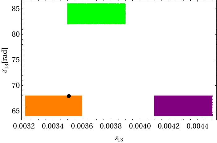
8.2 Step 2

In the next three years, LHCb should be able to provide good data on $S_{\psi\phi}$ and ${\rm Br}(B_{s}\to\mu^{+}\mu^{-})$ . As we have seen in Fig. 5, a measurement of $S_{\psi\phi}$ above 0.5 accompanied by ${\rm Br}(B_{s}\to\mu^{+}\mu^{-})_{\text{exp}}\leq{\rm Br}(B_{s}\to\mu^{+}\mu^{-})_{SM}$ would put the SM4 under pressure. Similarly for SM3-like values of $S_{\psi\phi}$ , ${\rm Br}(B_{s}\to\mu^{+}\mu^{-})$ can only be slightly enhanced over its SM3 value, and in fact a suppression of the latter branching ratio is more likely in this case.

In view of this pattern, we considered three scenarios shown in Table 4 and asked what they would imply for other decays. The result of this exercise is shown in all plots of Section 7 where the three scenarios of Table 4 are exhibited in three different colours indicated in this table. Alternatively, the colour coding can be conveniently inferred from Fig. 5. This results are self-explanatory and have been briefly discussed already in Section 7. Let us then only summarise our observations:

•

As seen in Fig. 3, the $S_{\phi K_{S}}$ and $S_{\psi K_{S}}$ anomalies can only be explained in scenario BS3.
•

As seen in Fig. 4, in the BS1 and BS3 scenarios the branching ratio ${\rm Br}(B_{d}\to\mu^{+}\mu^{-})$ remains SM3-like, while in scenario BS2 it can be enhanced by a factor of two.
•

As seen in Figs. 7 and 9 in all three scenarios large NP effects in ${\rm Br}(K^{+}\rightarrow\pi^{+}\nu\bar{\nu})$ , ${\rm Br}(K_{L}\rightarrow\pi^{0}\nu\bar{\nu})$ and ${\rm Br}(K_{L}\to\mu^{+}\mu^{-})$ are possible. Moreover in scenario BS3 they are particularly strongly correlated with each other.
•

For large positive values of $S_{\psi\phi}$ the predicted value of $\varepsilon^{\prime}/\varepsilon$ is significantly below the data, unless the hadronic matrix elements of the electroweak penguins are sufficiently suppressed with respect to the large $N$ result and the ones of QCD penguins enhanced.

This analysis shows that we will learn a lot about the SM4 when $S_{\psi\phi}$ , ${\rm Br}(B_{s}\to\mu^{+}\mu^{-})$ , ${\rm Br}(K^{+}\rightarrow\pi^{+}\nu\bar{\nu})$ and ${\rm Br}(K_{L}\rightarrow\pi^{0}\nu\bar{\nu})$ will be precisely known.

9 Determining the $V_{\text{SM4}}$ matrix

9.1 Preliminaries

As discussed in previous sections, the mixing between the third and fourth generation is bounded by the electroweak precision data and cannot be significantly larger than $s_{12}$ . Similarly, $s_{14}$ and $s_{24}$ are bounded by (2.47). As a consequence, as can be explicitly seen by the generalised Wolfenstein expansion for our benchmark scenarios (2.53–2.56), the relation between CKM parameters and the matrix elements $V_{us},V_{cd},V_{ub},V_{cb}$ ,

	$\displaystyle s_{12}$	$\displaystyle=\lambda\simeq\|V_{us}\|\simeq\|V_{cd}\|\,,\hskip 11.49994pt$	$\displaystyle s_{23}$	$\displaystyle=A\lambda^{2}\simeq\|V_{cb}\|\,,$		(9.1)
	$\displaystyle s_{13}$	$\displaystyle=A\lambda^{3}\|z_{\rho}\|\simeq\|V_{ub}\|\,,\hskip 11.49994pt$	$\displaystyle\delta_{13}$	$\displaystyle=-\text{arg}(z_{\rho})\simeq-\text{arg}(V_{ub})\,,$		(9.2)

are to a very good approximation unaffected by 4G contributions. Therefore the SM3 CKM parameters can be determined from the corresponding tree-level decays, practically without any NP pollution, with $\delta_{13}$ determined from $B\rightarrow DK$ . In particular such a determination does not require the $3\times 3$ CKM matrix to be unitary.⁶⁶ 6 Needless to say, $|V_{us}|,|V_{ub}|,|V_{cb}|$ and $\delta_{13}$ can be determined from tree-level decays even in the absence of this approximation, but the relation to the fundamental parameters is less transparent and involves the 4G parameters. In the present section we will further use (2.50) for the 4G mixing angles, in order to indicate how the $V_{\rm SM4}$ matrix can, in principle, be determined from future data.

A further comment on the determination of $\delta_{13}\approx\gamma$ is in order.

In the approximation of neglecting the phase of $V_{cs}$ and $V_{cb}$ , being real in the CKM convention, the $B_{s}\to D_{s}K$ complex in the SM3 measures directly a linear combination of the phase $\gamma$ and the phase of $B_{s}$ -mixing, where the latter can be extracted from $S_{\psi\phi}$ . Analogous comments apply to $B_{d}\to D\pi$ decays. In the presence of 4G quarks, the phases in $B_{s}$ and $B_{d}$ mixing may change, but again they can be determined from the $S_{\psi\phi}$ and $S_{\psi K_{S}}$ asymmetries, respectively. The new feature, as seen in (2.42), are new phases of $V_{cb}$ and $V_{cs}$ induced by the presence of the 4G quarks. However, the imposition of tree-level and electroweak precision constraints implies that this NP pollution amounts to significantly less than $1^{\circ}$ in the determination of $\delta_{13}$ and can be safely neglected. Analogous comments apply to other tree-level methods for the determination of $\delta_{13}$ .

The determination of the new parameters in the $V_{\text{SM4}}$ matrix,

s_{14}\,,\hskip 22.99988pts_{24}\,,\hskip 22.99988pts_{34}\,,\hskip 22.99988pt\delta_{14}\,,\hskip 22.99988pt\delta_{24}\,,

(9.3)

is probably beyond the scope of flavour-violating high-energy processes explored at the LHC and will have to be made through FCNC processes that, as in the SM3, appear first at the one-loop level due to the GIM mechanism at work. The accuracy of this determination will depend on

i)

the precision of the relevant experimental data,
ii)

the theoretical cleanliness of the observables involved (i.e. observables with small hadronic uncertainties should be favoured),
iii)

the potential size of NP contributions to the considered observable.

Clearly, the room for NP contributions to observables that are known already precisely will depend on the values of the CKM parameters in (9.2). In this context, let us recall the existing tension between the experimental values of $\varepsilon_{K}$ and $S_{\psi K_{S}}$ within the SM3 that has been extensively discussed in [139, 61, 146, 147]. Whether the SM3 has a problem with $\varepsilon_{K}$ , $S_{\psi K_{S}}$ or both observables depends on the values in (9.2). In turn, this will have an impact on the determination of the new parameters in (9.3). In what follows, we will first make a list of observables that could help us in the future to determine the parameters (9.3), subsequently illustrating such determinations on a few examples. A more extensive general numerical analysis appears to us to be premature at present. On the other hand, as we will see in Section 9.3, new insight can be gained by examining the anatomy of different scaling scenarios for the mixing angles and their implications for various flavour observables.

9.2 Basic Observables

Among the FCNC observables that have already been measured, the values for

\varepsilon_{K}\,,\hskip 22.99988pt\Delta M_{d}/\Delta M_{s}\,,\hskip 22.99988ptS_{\psi K_{S}}\,,\hskip 22.99988pt{\rm Br}\left(B\rightarrow X_{s}\gamma\right)

(9.4)

have presently the dominant impact on the allowed structure of the $V_{\text{SM4}}$ matrix. Indeed, $S_{\psi K_{S}}$ is theoretically very clean (see also the comment before Eq. (2.61)), and the hadronic uncertainties in $\varepsilon_{K}$ and $\Delta M_{d}/\Delta M_{s}$ are below $5\%$ already now and are expected to be decreased further in the coming years through improved lattice calculations.

Of particular interest in this decade will be the measurements of the branching ratios for

B_{s,d}\rightarrow\mu^{+}\mu^{-}\,,\hskip 22.99988ptK^{+}\rightarrow\pi^{+}\nu\bar{\nu}\,,\hskip 22.99988ptK_{L}\rightarrow\pi^{0}\nu\bar{\nu}\,,\hskip 22.99988ptB\rightarrow X_{s}\nu\bar{\nu}\,,

(9.5)

and, very importantly, of the CP-violating observables

S_{\psi\phi}\,,\hskip 22.99988ptS_{\phi K_{S}}\,,\hskip 22.99988ptA_{\text{CP}}(b\to s\gamma)\,.

(9.6)

In particular, various correlations between all these observables will significantly constrain the allowed range of the SM4 parameters and even have the power to exclude this NP scenario. Assuming that the SM4 will survive these new tests and having at hand all these measurements, it will be possible to determine the matrix $V_{\text{SM4}}$ . Indeed, let us note on the basis of the formulae of Section 4 that all these observables depend on six complex variables involving new parameters (see (2.57)),

\lambda^{(K)}_{t^{\prime}}\,,\hskip 22.99988pt\lambda^{(s)}_{t^{\prime}}\,,\hskip 22.99988pt\lambda^{(d)}_{t^{\prime}}\,,\hskip 22.99988pt\lambda^{(K)}_{t}\,,\hskip 22.99988pt\lambda^{(s)}_{t}\,,\hskip 22.99988pt\lambda^{(d)}_{t}\,,

(9.7)

that are not fully independent as, with (9.2) being fixed, they depend on the five parameters in (9.3). It is instructive to write down the expressions for $\lambda^{(i)}_{t^{(^{\prime})}}$ setting $c_{ij}=1$ and neglecting higher-order terms in the Wolfenstein expansion, leading to

$\displaystyle\lambda_{t^{\prime}}^{(d)}=V^{*}_{t^{\prime}b}V_{t^{\prime}d}$	$\displaystyle\approx\left(s_{34}+s_{13}s_{14}e^{i\left(\delta_{13}-\delta_{14}\right)}+s_{23}s_{24}e^{-i\delta_{24}}\right)$	(9.8)
	$\displaystyle\hskip 22.99988pt\times(e^{i\delta_{14}}s_{14}-e^{i\delta_{24}}s_{12}s_{24}-e^{i\delta_{13}}s_{13}s_{34}+s_{12}s_{23}s_{34})$	(9.9)
	$\displaystyle\approx-e^{i\delta_{13}}s_{13}s_{34}^{2}+s_{34}\left(s_{14}e^{i\delta_{14}}-s_{12}s_{24}e^{i\delta_{24}}\right)$	(9.10)
	$\displaystyle\hskip 22.99988pt+s_{14}s_{23}s_{24}e^{i\left(\delta_{1,4}-\delta_{24}\right)}-s_{12}s_{23}\left(s_{24}^{2}-s_{34}^{2}\right)\,,$	(9.11)
$\displaystyle\lambda_{t^{\prime}}^{(s)}=V^{*}_{t^{\prime}b}V_{t^{\prime}s}$	$\displaystyle\approx\left(s_{34}+s_{13}s_{14}e^{i\left(\delta_{13}-\delta_{14}\right)}+s_{23}s_{24}e^{-i\delta_{24}}\right)$	(9.12)
	$\displaystyle\hskip 22.99988pt\times(e^{i\delta_{24}}s_{24}+e^{i\delta_{14}}s_{12}s_{14}-s_{23}s_{34})$	(9.13)
	$\displaystyle\approx s_{12}s_{14}s_{34}e^{i\delta_{14}}+s_{24}s_{34}e^{i\delta_{24}}+s_{23}\left(s_{24}^{2}-s_{34}^{2}\right)\,,$	(9.14)
$\displaystyle\lambda_{t^{\prime}}^{(K)}=V^{*}_{t^{\prime}s}V_{t^{\prime}d}$	$\displaystyle\approx(e^{-i\delta_{24}}s_{24}+e^{-i\delta_{14}}s_{12}s_{14}-s_{23}s_{34})$	(9.15)
	$\displaystyle\hskip 22.99988pt\times(e^{i\delta_{14}}s_{14}-e^{i\delta_{24}}s_{12}s_{24}-e^{i\delta_{13}}s_{13}s_{34}+s_{12}s_{23}s_{34})$	(9.16)
	$\displaystyle\approx s_{24}\left(-s_{12}s_{24}+s_{14}e^{i\left(\delta_{14}-\delta_{24}\right)}\right)-s_{24}s_{34}e^{-i\delta_{24}}\left(-s_{12}s_{23}+s_{13}e^{i\delta_{13}}\right)$	(9.17)
	$\displaystyle\hskip 22.99988pt+\left(s_{12}s_{24}e^{i\delta_{24}}-s_{14}e^{i\delta_{14}}\right)\left(s_{23}s_{34}-s_{12}s_{14}e^{-i\delta_{14}}\right)$	(9.18)
	$\displaystyle\approx\frac{\lambda_{t^{\prime}}^{(s)\ast}\lambda_{t^{\prime}}^{(d)}}{\|V_{t^{\prime}b}\|^{2}}\,,$	(9.19)
$\displaystyle\lambda_{t}^{(d)}=V^{*}_{tb}V_{td}$	$\displaystyle\approx-s_{13}e^{i\delta_{13}}-s_{14}s_{34}e^{i\delta_{14}}+s_{12}\left(s_{23}+s_{24}s_{34}e^{i\delta_{24}}\right)$	(9.20)
	$\displaystyle\approx-s_{13}e^{i\delta_{13}}+s_{12}s_{23}-\lambda_{t^{\prime}}^{(d)}\,,$	(9.21)
$\displaystyle\lambda_{t}^{(s)}=V^{*}_{tb}V_{ts}$	$\displaystyle\approx-s_{23}-s_{24}s_{34}e^{i\delta_{24}}$	(9.22)
	$\displaystyle\approx-s_{23}-\lambda_{t^{\prime}}^{(s)}\,,$	(9.23)
$\displaystyle\lambda_{t}^{(K)}=V^{*}_{ts}V_{td}$	$\displaystyle\approx\left(s_{23}+s_{24}s_{34}e^{-i\delta_{24}}\right)$	(9.24)
	$\displaystyle\hskip 22.99988pt\times\left(s_{13}e^{i\delta_{13}}+s_{14}s_{34}e^{i\delta_{14}}-s_{12}\left(s_{23}+s_{24}s_{34}e^{i\delta_{24}}\right)\right)$	(9.25)
	$\displaystyle\approx\lambda_{t}^{(s)\ast}\lambda_{t}^{(d)}\,.$	(9.26)

We observe that, in general, the variables $\lambda_{t^{(^{\prime})}}^{(K,s,d)}$ involve all 5 mixing parameters associated with the 4G in a rather complicated way. Some simplification arises if we assume a certain scaling of the mixing angles $\theta_{i4}$ , for instance with one of our benchmark scenarios of Section 2. Let us, as an example, study the case (2.1), for which the above equations simplify as follows:

$\displaystyle\lambda_{t^{\prime}}^{(s)}$	$\displaystyle\approx e^{i\delta_{24}}s_{24}s_{34}\equiv\sigma_{23}\,,$	(9.27)
$\displaystyle\lambda_{t^{\prime}}^{(d)}$	$\displaystyle\approx s_{34}\left(s_{14}e^{i\delta_{14}}-s_{12}s_{24}e^{i\delta_{24}}\right)\equiv\sigma_{13}-s_{12}\sigma_{23}$	(9.28)
$\displaystyle\lambda_{t^{\prime}}^{(K)}$	$\displaystyle\approx s_{24}\left(-s_{12}s_{24}+s_{14}e^{i\left(\delta_{14}-\delta_{24}\right)}\right)=\frac{1}{s_{34}^{2}}\sigma_{23}^{\ast}\ (\sigma_{13}-s_{12}\sigma_{23})\hskip 11.49994pt[=\frac{1}{s_{34}^{2}}\lambda_{t^{\prime}}^{(s)\ast}\lambda_{t^{\prime}}^{(d)}]\,,$	(9.29)
$\displaystyle\lambda_{t}^{(s)}$	$\displaystyle\approx-s_{23}-s_{24}s_{34}e^{i\delta_{24}}=-s_{23}-\lambda_{t^{\prime}}^{(s)}\,,$	(9.30)
$\displaystyle\lambda_{t}^{(d)}$	$\displaystyle\approx-s_{13}e^{i\delta_{13}}-s_{14}s_{34}e^{i\delta_{14}}+s_{12}\left(s_{23}+s_{24}s_{34}e^{i\delta_{24}}\right)=-s_{13}e^{i\delta_{13}}+s_{12}s_{23}-\lambda_{t^{\prime}}^{(d)}\,,$	(9.31)
$\displaystyle\lambda_{t}^{(K)}$	$\displaystyle\approx\left(s_{23}+s_{24}s_{34}e^{-i\delta_{24}}\right)\left(s_{13}e^{i\delta_{13}}+s_{14}s_{34}e^{i\delta_{14}}-s_{12}\left(s_{23}+s_{24}s_{34}e^{i\delta_{24}}\right)\right)$	(9.32)
	$\displaystyle=\left(s_{23}+\lambda_{t^{\prime}}^{(s)\ast}\right)\left(s_{13}e^{i\delta_{13}}-s_{12}s_{23}+\lambda_{t^{\prime}}^{(d)}\right)\,,$	(9.33)

where the following two combinations of new parameters (9.3) have been introduced:

\displaystyle\sigma_{13}\equiv s_{14}s_{34}e^{i\delta_{14}}\,,\hskip 22.99988pt\sigma_{23}\equiv s_{24}s_{34}e^{i\delta_{24}}\,.

(9.34)

For this particular case, we observe that

i)

$\lambda^{(K)}_{t}$ and $\lambda^{(K)}_{t^{\prime}}$ depend on $\sigma_{13}$ , $\sigma_{23}$ and $s_{34}$ .
ii)

$\lambda^{(d)}_{t}$ and $\lambda^{(d)}_{t^{\prime}}$ depend on $\sigma_{13}$ and $\sigma_{23}$ .
iii)

$\lambda^{(s)}_{t}$ and $\lambda^{(s)}_{t^{\prime}}$ are sensitive to $\sigma_{23}$ only. The determination of $\Delta M_{s}$ , ${\rm Br}(B_{s}\rightarrow\mu^{+}\mu^{-})$ and $S_{\psi\phi}$ will thus play an important role in constraining these parameters. Moreover for ${s_{24}}\gtrsim{s_{23}}{s_{34}}$ and ${\delta_{24}}$ not too small, $S_{\psi\phi}$ should be much larger than its SM3 value $\left(S_{\psi\phi}\right)_{SM}\approx 0.04$ as we have seen in Section 7.

In view of the many possibilities for theoretical parameters and phenomenological observables, we will in the following develop a general procedure that allows us to analyse future experimental data in a systematic manner. Let us first consider the plots in Fig. 21, which show correlations between various parameters of the SM4, on the basis of the three scenarios of Table 4. In particular,

•

in the case of the scenario BS3 of Table 4, there is a strong correlation between $s_{24}$ and $s_{14}$ with $s_{24}\sim 4s_{14}$ and $s_{24}$ in the range

$\displaystyle 0.046\leq s_{24}\leq 0.17\,.$ (9.35)
•

$\delta_{14}$ and $\delta_{24}$ are also very strongly correlated in the BS3 scenario with $\delta_{14}\approx\delta_{24}\approx 270^{\circ}\pm 20^{\circ}$ .
•

in the lower left panel of Fig. 21 one can see the strong correlation (2.47) of $s_{34}$ and $m_{t^{\prime}}$ . We checked numerically that treating the EWPT in this approximate manner indeed gives reasonable bounds on $m_{t^{\prime}}$ .

In the following section, we will analyse these correlations within specific scaling scenarios for the 4G mixing angles.

9.3 Anatomy of 4G mixing angles and CP phases

As explained in Section 2, the 4G mixing matrix allows for different scalings of the 4G mixing angles $\theta_{14}$ , $\theta_{24}$ and $\theta_{34}$ with the Wolfenstein parameter $\lambda\ll 1$ . Among the set of parameters that fulfil the present constraints on flavour observables, we may thus classify different subsets by calculating the exponents

(n_{1},n_{2},n_{3})=\mbox{round}\left(\log_{\lambda}\left[\theta_{14},\theta_{24},\theta_{34}\right]\right)\,,

(9.36)

in (2.52) for $\lambda=s_{12}\ll 1$ . Furthermore (see also Fig. 21), for a given set $(n_{1},n_{2},n_{3})$ , the allowed values for the new CP phases $\delta_{14}$ and $\delta_{24}$ also exhibit a more or less strong correlation, which we will exploit to further distinguish different regions in the 4G parameter space. This enables us to identify a set of equivalence classes which – as we will illustrate – share certain characteristic features for the corresponding predictions for various flavour observables.

$(n_{1},n_{2},n_{3})$	Correlation $\delta_{24}$ vs. $\delta_{14}$	Assignment
$(2,1,1)$ $(2,2,1)$		$\to\left\{\begin{array}[]{ll}\mbox{\color[rgb]{0,0,1} class 1a:}&\color[rgb]{0,0,0}\delta_{14}<\delta_{24}<\delta_{14}+\frac{\pi}{8},\hskip 9.19995pt\delta_{24}<0.\\ \mbox{\color[rgb]{0.6,0.7,0} class 1b:}&\color[rgb]{0,0,0}\delta_{14}-\frac{\pi}{8}<\delta_{24}<\delta_{14},\hskip 9.19995pt\delta_{24}<0.\\ \mbox{\color[rgb]{1,0,1} class 2a:}&\color[rgb]{0,0,0}\delta_{14}<\delta_{24}<\delta_{14}+\frac{\pi}{8},\hskip 9.19995pt\delta_{24}>0.\\ \mbox{\color[rgb]{0,1,0} class 2b:}&\color[rgb]{0,0,0}\delta_{14}-\frac{\pi}{8}<\delta_{24}<\delta_{14},\hskip 9.19995pt\delta_{24}>0.\end{array}\right.$
$(3,2,1)$		$\to\left\{\begin{array}[]{ll}\mbox{\color[rgb]{0,0,1} class 1a:}&\color[rgb]{0,0,0}\delta_{14}<\delta_{24}<\delta_{14}+\frac{\pi}{8},\hskip 9.19995pt\delta_{24}<0.\\ \mbox{\color[rgb]{1,0,1} class 2a/3a:}&\color[rgb]{0,0,0}\delta_{14}<\delta_{24}<\delta_{14}+\frac{3\pi}{8},\ \ \delta_{24}>0.\\ \mbox{\color[rgb]{0.6,0.7,0} class 3b:}&\color[rgb]{0,0,0}\delta_{14}-\frac{3\pi}{8}<\delta_{24}<\delta_{14}.\end{array}\right.$
$(3,3,1)$ $(3,3,2)$		$\to\left\{\begin{array}[]{ll}\mbox{\color[rgb]{1,0,1} class 3a:}&\color[rgb]{0,0,0}\delta_{14}+\frac{\pi}{8}<\delta_{24}<\delta_{14}+\frac{\pi}{2}.\\ \mbox{\color[rgb]{0.6,0.7,0} class 3b:}&\delta_{14}-\frac{3\pi}{4}<\delta_{24}<\delta_{14}.\\ \mbox{\color[rgb]{0,1,0} class 4:}&\delta_{14}-\frac{9\pi}{8}<\delta_{24}<\delta_{14}-\frac{3\pi}{4}.\end{array}\right.$
$(4,3,1)$ $(4,3,2)$		$\to\left\{\begin{array}[]{ll}\mbox{\color[rgb]{0,0,1} class 5:}&\delta_{14}-\frac{3\pi}{2}<\delta_{24}<\delta_{14}+\frac{\pi}{4}\end{array}\right.$
$(2,3,1)$		$\to\left\{\begin{array}[]{ll}\mbox{\color[rgb]{1,0,1} class 6:}&\delta_{14}+\frac{\pi}{8}<\delta_{24}<\delta_{14}+\frac{3\pi}{4}.\\ \mbox{\color[rgb]{0.6,0.7,0} class 7:}&\delta_{14}-\frac{9\pi}{8}<\delta_{24}<\delta_{14}-\frac{\pi}{4}.\end{array}\right.$

Table 8: Correlations between 4G phases for different scalings of 4G mixing angles (some selected examples). The constraints on the phases, of course, are understood to be periodic in units of

2\pi

According to our discussion above, values $(n_{1},n_{2},n_{3})$ that do not fulfil the inequalities (2.20), from the theoretical point of view, should be considered as fine-tuned and will not be included in the subsequent discussion. (We convinced ourselves that we do not miss any of the observed phenomenological features by doing so.) For the remaining cases, we first identify – for a given scaling $(n_{1},n_{2},n_{3})$ – the allowed correlations between $\delta_{14}$ and $\delta_{24}$ , and then determine the assignment to one or the other equivalence class. Our procedure is summarised for the most prominent and representative examples in Table 8:

•

Evidently, for small values of the $n_{i}$ (i.e. large values of 4G mixing angles), one expects the largest deviations from the SM3 predictions. In fact, the most extreme case is characterised by example (2.1) from Section 2, with values $(n_{1},n_{2},n_{3})=(2,1,1)$ . As we already discussed, in this scenario the new 4G phases contribute at leading order to CP-violating observables, and therefore $\delta_{14}$ and $\delta_{24}$ are highly correlated and constrained. Separating the different relative and absolute signs of $\delta_{i4}$ enables us to classify the subsets $1a,1b,2a,2b$ which show characteristic features in the selected set of observables shown in Tables 9+10. Similar correlations are found for the $(2,2,1)$ scenario.
•

Decreasing the values of (some of) the mixing angles (i.e. increasing $n_{1},n_{2},n_{3}$ ), we observe that the correlations between the 4G phases become broader. Still, the values populate restricted areas in the $\delta_{24}$ – $\delta_{14}$ plane, which again allows to identify sub-classes with definite properties. A typical example is the case $(3,2,1)$ from our benchmark scenario (2.1). This scenario divides into two well-separated regions. Among one of them, we may (or may not) identify a subset of points as belonging to class 1a. This kind of arbitrariness is unavoidable (and expected), since the separation of points from scenario $(2,2,1)$ and $(3,2,1)$ is not clear-cut.
•

For even smaller values of mixing angles, we observe for the cases $(3,3,1)$ and $(3,3,2)$ a separation into three sub-classes, where two classes (3a and 3b) can be considered as a continuation of those from the $(3,2,1)$ scenario, and class 4 is new.
•

Considering $(4,3,1)$ (the benchmark scenario (2.1) discussed in Section 2) and $(4,3,2)$ , the former classes 3b and 4 merge into one class 5 which already covers around half of the $\delta_{24}$ - $\delta_{14}$ plane. Finally, for the scenario (2.1) with the scaling $(2,3,1)$ , the former class 3a continues into class 6, while 3b and 4 merge into class 7, where the parameter space in the $\delta_{24}$ - $\delta_{14}$ plane is again somewhat more constrained.

Having identified the different sub-classes, we investigate the characteristic features for certain phenomenological observables in Tables 9-12. We see that each class can be distinguished from the others by at least one of the shown correlations: ${\rm Br}(B_{s}\to\mu^{+}\mu^{-})$ vs. $S_{\psi\phi}$ , $S_{\phi K_{S}}$ vs. $S_{\psi\phi}$ , ${\rm Br}(b\to s\gamma)$ vs. ${\rm Br}(B\to X_{s}\ell\ell)$ , ${\rm Br}(K_{L}\to\mu^{+}\mu^{-})_{\rm SD}$ vs. ${\rm Br}(K^{+}\to\pi^{+}\nu\bar{\nu})$ (The colour-coding is as defined in Table 4).

Turning the argument around, the observation of a combination of particular correlations in rare flavour processes can be translated into one or the other favoured scenario for 4G mixing angles and CP phases. Only after a particular scaling scenario has been identified, the formulae for $\lambda_{t^{\prime}}^{(K,d,s)}$ in (9.15–9.22) can be simplified, and we may (more or less) unambiguously determine the 4G mixing parameters from the future experimental data. We emphasise that, quite generally, such a procedure should be applied to the analysis of flavour parameters in NP models without MFV. In particular, without a specific theory of flavour at hand, the fact that certain scaling scenarios – like (2.1) – are represented by only a small number of points in the overall scan of parameter space, should not be taken as a signal for a small probability to observe the associated correlations in flavour observables.

[Uncaptioned image] — Table 9: Selected correlations for classes identified in Table 8 (part 1 of 4). (The colour-coding is as defined in Table 4).

10 Summary and Conclusions

In the present paper we have performed a detailed analysis of non-MFV effects in the $K$ , $B_{d}$ and $B_{s}$ systems in the SM4, paying particular attention to correlations between various flavour observables and addressing within this framework a number of anomalies present in the experimental data.

Similarly as in the LHT model, the RSc model and supersymmetric flavour models that have been analysed in [31, 32, 33, 34, 35, 36], the correlations between various observables that are characteristic for models with MFV and in particular with CMFV can be strongly violated in the SM4 while still satisfying all existing data on flavour violating processes and electroweak precision observables.

Probably, the most striking signature of the SM4, compared to the LHT, RSc and SUSY flavour models, is the possibility of having simultaneously sizable NP effects in the $K$ , $B_{d}$ and $B_{s}$ systems, even if truly spectacular effects are only possible in rare $K$ decays with the prominent exception of $S_{\psi\phi}$ which can also be enhanced by an order of magnitude. This different pattern can be traced back to the fact that the mass scales involved in the SM4 are generally significantly lower than in the LHT and in particular in the RSc. Also the non-decoupling of the new heavy fermions $t^{\prime}$ and $b^{\prime}$ plays a role here, whereas an analogous effect does not occur in the LHT, RSc and SUSY.

We recall that in SUSY flavour models, NP effects in the $K$ system are small but can be large in $B$ physics observables to which dipole operators and scalar operators contribute. In models with right-handed currents also $S_{\psi\phi}$ can be large. In the LHT and RSc models, large effects are found predominantly in rare $K$ decays, although $S_{\psi\phi}$ can also be sizable. These three different global patterns of flavour violation in the models in question could help one day to distinguish between these NP scenarios.

The most interesting patterns of flavour violation in the SM4 are the following ones.

•

All existing tensions in the UT fits can be removed in this NP scenario.
•

In particular the desire to explain the $S_{\psi\phi}$ anomaly implies, as seen in Fig. 3, uniquely the suppressions of the CP asymmetries $S_{\phi K_{S}}$ and $S_{\eta^{\prime}K_{S}}$ in agreement with the data. This correlation has been pointed out in [15, 148, 149], and we confirm it here. However we observe that for $S_{\psi\phi}$ significantly larger than 0.6 the values of $S_{\phi K_{s}}$ and $S_{\eta^{\prime}K_{s}}$ are below their central values indicated by the data.
•

The same anomaly implies a sizable enhancement of ${\rm Br}(B_{s}\to\mu^{+}\mu^{-})$ over the SM3 prediction although this effect is much more modest than in SUSY models where the Higgs penguin with large $\tan\beta$ is at work. Yet, values as high as $8\cdot 10^{-9}$ are certainly possible in the SM4, which is well beyond those attainable in the LHT model and the RSc model.
•

Possible enhancements of ${\rm Br}(K^{+}\rightarrow\pi^{+}\nu\bar{\nu})$ and ${\rm Br}(K_{L}\rightarrow\pi^{0}\nu\bar{\nu})$ over the SM3 values are much larger than found in the LHT and RSc models and in particular in SUSY flavour models where they are SM3 like. Both branching ratios as high as several $10^{-10}$ are still possible in the SM4. Moreover, in this case, the two branching ratios are strongly correlated as seen in Fig. 7 and close to the GN bound. For an earlier analysis see [13].
•

Interestingly, in contrast to the LHT and RSc models, a high value of $S_{\psi\phi}$ does not preclude a sizable enhancements of ${\rm Br}(K^{+}\rightarrow\pi^{+}\nu\bar{\nu})$ , and ${\rm Br}(K_{L}\rightarrow\pi^{0}\nu\bar{\nu})$ .
•

NP effects in $K_{L}\to\pi^{0}\ell^{+}\ell^{-}$ and $K_{L}\to\mu^{+}\mu^{-}$ can be visibly larger than in the LHT and RSc models. In particular ${\rm Br}(K_{L}\to\mu^{+}\mu^{-})_{\rm SD}$ can easily violate the existing bound of $2.5\cdot 10^{-9}$ . Imposition of this bound on top of other constraints results in a characteristic shape of the correlation between ${\rm Br}(K^{+}\rightarrow\pi^{+}\nu\bar{\nu})$ and ${\rm Br}(K_{L}\rightarrow\pi^{0}\nu\bar{\nu})$ shown in Fig. 7.
•

The magnitude of the CP asymmetry $A_{\rm CP}^{bs\gamma}$ remains small, but the desire to explain large values of $S_{\psi\phi}$ reverses its sign.
•

Even in the presence of SM-like values for $S_{\psi\phi}$ and ${\rm Br}(B_{s}\to\mu^{+}\mu^{-})$ , large effects in the $K$ -system are possible as illustrated by green points in numerous plots.
•

For large positive values of $S_{\psi\phi}$ the predicted value of $\varepsilon^{\prime}/\varepsilon$ is significantly below the data, unless the hadronic matrix elements of the electroweak penguins are sufficiently suppressed with respect to the large $N$ result and the ones of QCD penguins enhanced.
•

We have also reemphasised [120, 121] the important role $\varepsilon^{\prime}/\varepsilon$ will play in bounding rare $K$ decay branching ratios once the relevant hadronic matrix elements in $\varepsilon^{\prime}/\varepsilon$ will be precisely known (see Sec. 7.12 for more details).

Other 4G effects in various observables and correlations between them can be found in numerous plots in Sections 7–9. In particular, in Section 9, we have addressed the question of the determination of the parameters of the SM4 with the help of future measurements employing various scenarios for the scalings of the 4G mixing matrix angles $\theta_{14},\theta_{24}$ and $\theta_{34}$ with the Wolfenstein parameter $\lambda\ll 1$ .

In summary, the SM4 offers a very rich pattern of flavour violation which can be tested already in the coming years, in particular through precise measurements of $S_{\psi\phi}$ , ${\rm Br}(B_{q}\to\mu^{+}\mu^{-})$ , ${\rm Br}(K^{+}\to\pi^{+}\nu\bar{\nu})$ and, later, $S_{\phi K_{s}}$ , $S_{\eta^{\prime}K_{s}}$ and ${\rm Br}(K_{L}\to\pi^{0}\nu\bar{\nu})$ . Also, precise measurements of the phase $\gamma\approx\delta_{13}$ will be important for this investigation. We close our detailed analysis with the following important question: Can the SM4 be excluded by precise measurements of FCNC processes? The answer is positive, provided large departures from the SM3 are observed with a different pattern of deviation from the SM3 predictions than found in our analysis. Let us just list three examples:

•

Large values of $S_{\psi\phi}>0.6$ accompanied with SM-like values of ${\rm Br}(B_{s}\to\mu^{+}\mu^{-})$ will clearly disfavour the SM4 as the explanation of the $S_{\psi\phi}$ anomaly.
•

Similarly, such large values accompanied by the observation of $S_{\phi K_{s}}\approx S_{\eta^{\prime}K_{s}}\approx S_{\psi K_{s}}$ would also put the SM4 into difficulties.
•

Finally, $S_{\psi\phi}>0.3$ accompanied by the $\varepsilon^{\prime}/\varepsilon$ relevant $R_{6}\approx R_{8}\approx 1$ from future lattice calculations will disfavour SM4 by means of the measured $\varepsilon^{\prime}/\varepsilon$ .

It is evident from our analysis and other analyses mentioned in the beginning of our paper that FCNC processes will contribute in a profound manner to the search for the 4G quarks and leptons and, in the case of direct discovery, to the exploration of the structure of their weak mixings. We hope that our numerous plots will help in monitoring the future data from LHC and high-intensity experiments, with the hope to firmly establish or firmly exclude the presence of the fourth sequential generation of quarks in nature.

Note added

Very recently, during the final stages of our work, a detailed study of rare $K$ and $B$ decays has been presented in [140], see also the discussion in Section 7.3.

Acknowledgements

We would like to thank Wolfgang Altmannshofer, Monika Blanke, Amarjit Soni and Soumitra Nandi for illuminating discussions. This research was partially supported by the Cluster of Excellence ‘Origin and Structure of the Universe’, the Graduiertenkolleg GRK 1054 of DFG and by the German ‘Bundesministerium für Bildung und Forschung’ under contract 05H09WOE.

Appendix A Relevant Functions

$\displaystyle X_{0}(x_{i})$	$\displaystyle=$	$\displaystyle\frac{x_{i}}{8}\;\left[\frac{x_{i}+2}{x_{i}-1}+\frac{3x_{i}-6}{(x_{i}-1)^{2}}\;\log x_{i}\right],$	(A.1)
$\displaystyle Y_{0}(x_{i})$	$\displaystyle=$	$\displaystyle\frac{x_{i}}{8}\;\left[\frac{x_{i}-4}{x_{i}-1}+\frac{3x_{i}}{(x_{i}-1)^{2}}\log x_{i}\right],$	(A.2)
$\displaystyle Z_{0}(x_{i})$	$\displaystyle=$	$\displaystyle-\frac{1}{9}\log x_{i}+\frac{18x_{i}^{4}-163x_{i}^{3}+259x_{i}^{2}-108x_{i}}{144(x_{i}-1)^{3}}$	(A.3)
		$\displaystyle+\frac{32x_{i}^{4}-38x_{i}^{3}-15x_{i}^{2}+18x_{i}}{72(x_{i}-1)^{4}}\log x_{i}\,.$	(A.3)
$\displaystyle C_{0}(x_{i})$	$\displaystyle=$	$\displaystyle\frac{x_{i}}{8}\left[\frac{x_{i}-6}{x_{i}-1}+\frac{3x_{i}+2}{(x_{i}-1)^{2}}\log x_{i}\right],$	(A.4)
$\displaystyle D_{0}(x_{i})$	$\displaystyle=$	$\displaystyle-\frac{4}{9}\log x_{i}+\frac{-19x_{i}^{3}+25x_{i}^{2}}{36(x_{i}-1)^{3}}+\frac{x_{i}^{2}(5x_{i}^{2}-2x_{i}-6)}{18(x_{i}-1)^{4}}\log x_{i}\,,$	(A.5)
$\displaystyle E_{0}(x_{i})$	$\displaystyle=$	$\displaystyle-\frac{2}{3}\log x_{i}+\frac{x_{i}^{2}(15-16x_{i}+4x_{i}^{2})}{6(x_{i}-1)^{4}}\log x_{i}+\frac{x_{i}(18-11x_{i}-x_{i}^{2})}{12(1-x_{i})^{3}}\,,$	(A.6)
$\displaystyle D^{\prime}_{0}(x_{i})$	$\displaystyle=$	$\displaystyle-\frac{(3x_{i}^{3}-2x_{i}^{2})}{2(x_{i}-1)^{4}}\log x_{i}+\frac{(8x_{i}^{3}+5x_{i}^{2}-7x_{i})}{12(x_{i}-1)^{3}}\,,$	(A.7)
$\displaystyle E^{\prime}_{0}(x_{i})$	$\displaystyle=$	$\displaystyle\frac{3x_{i}^{2}}{2(x_{i}-1)^{4}}\log x_{i}+\frac{(x_{i}^{3}-5x_{i}^{2}-2x_{i})}{4(x_{i}-1)^{3}}\,.$	(A.8)

	$\displaystyle B^{\mu\bar{\mu}}(x_{i},y_{j})$	$\displaystyle=$	$\displaystyle\frac{1}{4}\left[U(x_{i},y_{j})+\frac{x_{i}y_{j}}{4}U(x_{i},y_{j})-2x_{i}y_{j}\tilde{U}(x_{i},y_{j})\right]\,,$		(A.9)
	$\displaystyle B^{\nu\bar{\nu}}(x_{i},y_{j})$	$\displaystyle=$	$\displaystyle\frac{1}{4}\left[U(x_{i},y_{j})+\frac{x_{i}y_{j}}{16}U(x_{i},y_{j})+\frac{x_{i}y_{j}}{2}\tilde{U}(x_{i},y_{j})\right]\,,$		(A.10)

with

	$\displaystyle U(x_{1},x_{2})$	$\displaystyle=$	$\displaystyle\frac{x_{1}^{2}\log x_{1}}{(x_{1}-x_{2})(1-x_{1})^{2}}+\frac{x_{2}^{2}\log x_{2}}{(x_{2}-x_{1})(1-x_{2})^{2}}+\frac{1}{(1-x_{1})(1-x_{2})}\,,$		(A.11)
	$\displaystyle\tilde{U}(x_{1},x_{2})$	$\displaystyle=$	$\displaystyle\frac{x_{1}\log x_{1}}{(x_{1}-x_{2})(1-x_{1})^{2}}+\frac{x_{2}\log x_{2}}{(x_{2}-x_{1})(1-x_{2})^{2}}+\frac{1}{(1-x_{1})(1-x_{2})}\,.$		(A.12)

$S_{0}(x_{i},x_{j})$ for arbitrary $x_{i},x_{j}$ is given by [59]

\displaystyle S_{0}(x_{i},x_{j})

\displaystyle=

\displaystyle x_{i}x_{j}\left(\frac{(4-8x_{j}+x_{j}^{2})\log x_{j}}{4(x_{j}-1)^{2}(x_{j}-x_{i})}+(i\leftrightarrow j)-\frac{3}{4(x_{i}-1)(x_{j}-1)}\right)\,.

(A.13)

In the limit of $\varepsilon\rightarrow 0$ in $S_{0}(x_{i}+\varepsilon,x_{i}-\varepsilon)$ one recovers the SM3 version of $S_{0}(x_{i})$ ,

\displaystyle S_{0}(x_{i})

\displaystyle=

\displaystyle\frac{x_{i}}{4}\;\frac{-4+15x_{i}-(12-6\log x_{i})x_{i}^{2}+x_{i}^{3}}{(x_{i}-1)^{3}}\,.

(A.14)

References

[1] P. H. Frampton, P. Q. Hung, and M. Sher, Quarks and leptons beyond the third generation, Phys. Rept. 330 (2000) 263, hep-ph/9903387 .
[2] M. Maltoni, V. A. Novikov, L. B. Okun, A. N. Rozanov, and M. I. Vysotsky, Extra quark-lepton generations and precision measurements, Phys. Lett. B476 (2000) 107–115, hep-ph/9911535 .
[3] H.-J. He, N. Polonsky, and S. fang Su, Extra families, Higgs spectrum and oblique corrections, Phys. Rev. D64 (2001) 053004, hep-ph/0102144 .
[4] J. Alwall et al., Is $V_{tb}\simeq 1$ ?, Eur. Phys. J. C49 (2007) 791–801, hep-ph/0607115 .
[5] G. D. Kribs, T. Plehn, M. Spannowsky, and T. M. P. Tait, Four generations and Higgs physics, Phys. Rev. D76 (2007) 075016, 0706.3718 .
[6] M. S. Chanowitz, Bounding CKM Mixing with a Fourth Family, Phys. Rev. D79 (2009) 113008, 0904.3570 .
[7] V. A. Novikov, A. N. Rozanov, and M. I. Vysotsky, Once more on extra quark-lepton generations and precision measurements, 0904.4570.
[8] M. Hashimoto, Constraints on Mass Spectrum of Fourth Generation Fermions and Higgs Bosons, 1001.4335.
[9] P. Q. Hung, Minimal SU(5) resuscitated by long-lived quarks and leptons, Phys. Rev. Lett. 80 (1998) 3000–3003, hep-ph/9712338 .
[10] W.-S. Hou, CP Violation and Baryogenesis from New Heavy Quarks, Chin. J. Phys. 47 (2009) 134, 0803.1234 .
[11] Y. Kikukawa, M. Kohda, and J. Yasuda, The strongly coupled fourth family and a first-order electroweak phase transition (I) Quark sector, Prog. Theor. Phys. 122 (2009) 401–426, 0901.1962 .
[12] R. Fok and G. D. Kribs, Four Generations, the Electroweak Phase Transition, and Supersymmetry, Phys. Rev. D78 (2008) 075023, 0803.4207 .
[13] W.-S. Hou, M. Nagashima, and A. Soddu, Enhanced $K_{L}\to\pi^{0}\nu\bar{\nu}$ from direct CP violation in $B\to K\pi$ with four generations, Phys. Rev. D72 (2005) 115007, hep-ph/0508237 .
[14] W.-S. Hou, M. Nagashima, and A. Soddu, Large time-dependent CP violation in $B_{s}^{0}$ system and finite $D^{0}$ - $\bar{D}^{0}$ mass difference in four generation standard model, Phys. Rev. D76 (2007) 016004, hep-ph/0610385 .
[15] A. Soni, A. K. Alok, A. Giri, R. Mohanta, and S. Nandi, The Fourth family: A Natural explanation for the observed pattern of anomalies in B–CP asymmetries, 0807.1971.
[16] G. Burdman, L. Da Rold, and R. D. Matheus, The Lepton Sector of a Fourth Generation, 0912.5219.
[17] B. Holdom, Heavy quarks and electroweak symmetry breaking, Phys. Rev. Lett. 57 (1986) 2496.
[18] C. T. Hill, M. A. Luty, and E. A. Paschos, Electroweak symmetry breaking by fourth generation condensates and the neutrino spectrum, Phys. Rev. D43 (1991) 3011–3025.
[19] S. F. King, Is electroweak symmetry broken by a fourth family of quarks? , Phys. Lett. B234 (1990) 108–112.
[20] G. Burdman and L. Da Rold, Electroweak Symmetry Breaking from a Holographic Fourth Generation, JHEP 12 (2007) 086, 0710.0623 .
[21] P. Q. Hung and C. Xiong, Renormalization Group Fixed Point with a Fourth Generation: Higgs-induced Bound States and Condensates, 0911.3890.
[22] P. Q. Hung and C. Xiong, Renormalization Group Fixed Point with a Fourth Generation: Solution to the hierarchy problem, 0911.3892.
[23] B. Holdom, Approaching a strong fourth family, Phys. Lett. B686 (2010) 146–151, 1001.5321 .
[24] B. Holdom et al., Four Statements about the Fourth Generation, 0904.4698.
[25] A. Arhrib and W.-S. Hou, Effect of fourth generation CP phase on $b\to s$ transitions, Eur. Phys. J. C27 (2003) 555–561, hep-ph/0211267 .
[26] J. A. Herrera, R. H. Benavides, and W. A. Ponce, Flavor changing neutral currents with a fourth family of quarks, Phys. Rev. D78 (2008) 073008, 0810.3871 .
[27] M. Bobrowski, A. Lenz, J. Riedl, and J. Rohrwild, How much space is left for a new family of fermions?, Phys. Rev. D79 (2009) 113006, 0902.4883 .
[28] G. Eilam, B. Melic, and J. Trampetic, CP violation and the 4th generation, Phys. Rev. D80 (2009) 116003, 0909.3227 .
[29] Z. Murdock, S. Nandi, and Z. Tavartkiladze, Perturbativity and a Fourth Generation in the MSSM, Phys. Lett. B668 (2008) 303–307, 0806.2064 .
[30] R. M. Godbole, S. K. Vempati, and A. Wingerter, Four Generations: SUSY and SUSY Breaking, 0911.1882.
[31] M. Blanke et al., Particle antiparticle mixing, $\epsilon_{K}$ , $\Delta(\Gamma(q))$ , $A_{\rm SL}(q)$ , $A_{\rm CP}(B_{d}\to\psi K_{S})$ , $A_{\rm CP}(B_{s}\to\psi\phi)$ and $B\to X_{s,d}\gamma$ in the littlest Higgs model with T-parity, JHEP 12 (2006) 003, hep-ph/0605214 .
[32] M. Blanke et al., Rare and CP-Violating $K$ and $B$ Decays in the Littlest Higgs Model with T-Parity, JHEP 01 (2007) 066, hep-ph/0610298 .
[33] M. Blanke, A. J. Buras, B. Duling, S. Recksiegel, and C. Tarantino, FCNC Processes in the Littlest Higgs Model with T-Parity: a 2009 Look, Acta Phys. Polon. B 41 (2010) 657, 0906.5454 .
[34] M. Blanke, A. J. Buras, B. Duling, S. Gori, and A. Weiler, $\Delta F=2$ Observables and Fine-Tuning in a Warped Extra Dimension with Custodial Protection, JHEP 03 (2009) 001, 0809.1073 .
[35] M. Blanke, A. J. Buras, B. Duling, K. Gemmler, and S. Gori, Rare $K$ and $B$ Decays in a Warped Extra Dimension with Custodial Protection, JHEP 03 (2009) 108, 0812.3803 .
[36] W. Altmannshofer, A. J. Buras, S. Gori, P. Paradisi, and D. M. Straub, Anatomy and Phenomenology of FCNC and CPV Effects in SUSY Theories, Nucl. Phys. B830 (2010) 17–94, 0909.1333 .
[37] G. D’Ambrosio, G. F. Giudice, G. Isidori, and A. Strumia, Minimal flavour violation: An effective field theory approach, Nucl. Phys. B645 (2002) 155–187, hep-ph/0207036 .
[38] T. Feldmann, M. Jung, and T. Mannel, Sequential Flavour Symmetry Breaking, Phys. Rev. D80 (2009) 033003, 0906.1523 .
[39] A. Santamaria, Masses, mixings, Yukawa couplings and their symmetries, Phys. Lett. B305 (1993) 90–97, hep-ph/9302301 .
[40] J. Berger and Y. Grossman, Parameter counting in models with global symmetries, Phys. Lett. B675 (2009) 365–370, 0811.1019 .
[41] T. Feldmann and T. Mannel, Minimal Flavour Violation and Beyond, JHEP 02 (2007) 067, hep-ph/0611095 .
[42] T. Feldmann and T. Mannel, Large Top Mass and Non-Linear Representation of Flavour Symmetry, Phys. Rev. Lett. 100 (2008) 171601, 0801.1802 .
[43] A. L. Kagan, G. Perez, T. Volansky, and J. Zupan, General Minimal Flavor Violation, Phys. Rev. D80 (2009) 076002, 0903.1794 .
[44] C. D. Froggatt and H. B. Nielsen, Hierarchy of Quark Masses, Cabibbo Angles and CP Violation, Nucl. Phys. B147 (1979) 277.
[45] H. Fritzsch and J. Plankl, The Mixing of Quark Flavors, Phys. Rev. D35 (1987) 1732.
[46] H. Harari and M. Leurer, Recommending a Standard Choice of Cabibbo Angles and KM Phases for Any Number of Generations, Phys. Lett. B181 (1986) 123.
[47] A. A. Anselm, J. L. Chkareuli, N. G. Uraltsev, and T. A. Zhukovskaya, On the Kobayashi-Maskawa model with four generations, Phys. Lett. B156 (1985) 102–108.
[48] L. Wolfenstein, Parametrization of the Kobayashi-Maskawa Matrix, Phys. Rev. Lett. 51 (1983) 1945.
[49] A. J. Buras, M. E. Lautenbacher, and G. Ostermaier, Waiting for the top quark mass, $K^{+}\to\pi^{+}\nu\bar{\nu}$ , $B_{s}^{0}-\bar{B}_{s}^{0}$ mixing and CP asymmetries in B decays, Phys. Rev. D50 (1994) 3433–3446, hep-ph/9403384 .
[50] W.-S. Hou, A. Soni, and H. Steger, Effects of a Fourth Family on $b\to s\gamma$ and a Useful Parametrization of Quark Mixing for Rare $B$ Decays, Phys. Lett. B192 (1987) 441.
[51] C. Jarlskog, Commutator of the Quark Mass Matrices in the Standard Electroweak Model and a Measure of Maximal CP Violation, Phys. Rev. Lett. 55 (1985) 1039.
[52] C. Jarlskog, A Basis Independent Formulation of the Connection Between Quark Mass Matrices, CP Violation and Experiment, Z. Phys. C29 (1985) 491–497.
[53] F. del Aguila and J. A. Aguilar-Saavedra, Invariant formulation of CP violation for four quark families, Phys. Lett. B386 (1996) 241–246, hep-ph/9605418 .
[54] G. Buchalla, A. J. Buras, and M. E. Lautenbacher, Weak Decays Beyond Leading Logarithms, Rev. Mod. Phys. 68 (1996) 1125–1144, hep-ph/9512380 .
[55] G. Buchalla and A. J. Buras, The rare decays $K\to\pi\nu\bar{\nu}$ , $B\to X\nu\bar{\nu}$ and $B\to\ell^{+}\ell^{-}$ : An update, Nucl. Phys. B548 (1999) 309–327, hep-ph/9901288 .
[56] M. Misiak and J. Urban, QCD corrections to FCNC decays mediated by Z-penguins and W-boxes, Phys. Lett. B451 (1999) 161–169, hep-ph/9901278 .
[57] M. Gorbahn and U. Haisch, Charm quark contribution to $K_{L}\to\mu^{+}\mu^{-}$ at next-to- next-to-leading order, Phys. Rev. Lett. 97 (2006) 122002, hep-ph/0605203 .
[58] G. Buchalla, A. J. Buras, and M. K. Harlander, Penguin box expansion: Flavor changing neutral current processes and a heavy top quark, Nucl. Phys. B349 (1991) 1–47.
[59] A. J. Buras, W. Slominski, and H. Steger, $B$ Meson Decay, CP Violation, Mixing Angles and the Top Quark Mass, Nucl. Phys. B238 (1984) 529.
[60] A. J. Buras, Weak Hamiltonian, CP violation and rare decays, hep-ph/9806471.
[61] A. J. Buras and D. Guadagnoli, Correlations among new CP violating effects in $\Delta F=2$ observables, Phys. Rev. D78 (2008) 033005, 0805.3887 .
[62] J. Laiho, R. S. Van de Water, and E. Lunghi, Lattice QCD inputs to the CKM unitarity triangle analysis, 0910.2928.
[63] A. J. Buras, D. Guadagnoli, and G. Isidori, On $\epsilon_{K}$ beyond lowest order in the Operator Product Expansion, 1002.3612.
[64] CDF Collaboration, T. Aaltonen et al., First Flavor-Tagged Determination of Bounds on Mixing-Induced CP Violation in $B^{0}_{s}\to J/\psi\phi$ Decays, Phys. Rev. Lett. 100 (2008) 161802, 0712.2397 .
[65] D0 Collaboration, V. M. Abazov et al., Measurement of $B^{0}_{s}$ mixing parameters from the flavor-tagged decay $B^{0}_{s}\to J/\psi\phi$ , Phys. Rev. Lett. 101 (2008) 241801, 0802.2255 .
[66] Heavy Flavor Averaging Group Collaboration, E. Barberio et al., Averages of $b-$ hadron and $c-$ hadron Properties at the End of 2007, 0808.1297.
[67] A. J. Buras, Relations between $\Delta M_{s,d}$ and $B_{s,d}\to\mu\bar{\mu}$ in models with minimal flavour violation, Phys. Lett. B566 (2003) 115–119, hep-ph/0303060 .
[68] J. Shigemitsu et al., Recent results on $B$ mixing and decay constants from HPQCD, 0910.4131.
[69] CDF Collaboration, T. Aaltonen et al., Search for $B^{0}_{s}\to\mu^{+}\mu^{-}$ and $B^{0}_{d}\to\mu^{+}\mu^{-}$ decays with $2fb^{-1}$ of $p\bar{p}$ collisions, Phys. Rev. Lett. 100 (2008) 101802, 0712.1708 .
[70] D0 Collaboration, V. M. Abazov et al., Search for $B_{s}\to\mu^{+}\mu^{-}$ at D0, Phys. Rev. D76 (2007) 092001, 0707.3997 .
[71] G. Punzi, Flavour physics at the Tevatron, 1001.4886.
[72] G. Isidori and R. Unterdorfer, On the short-distance constraints from $K_{L,S}\to\mu^{+}\mu^{-}$ , JHEP 01 (2004) 009, hep-ph/0311084 .
[73] P. Colangelo, F. De Fazio, P. Santorelli, and E. Scrimieri, Rare $B\to K^{*}\nu\bar{\nu}$ decays at $B$ factories, Phys. Lett. B395 (1997) 339–344, hep-ph/9610297 .
[74] G. Buchalla, G. Hiller, and G. Isidori, Phenomenology of non-standard Z couplings in exclusive semileptonic $b\to s$ transitions, Phys. Rev. D63 (2001) 014015, hep-ph/0006136 .
[75] W. Altmannshofer, A. J. Buras, D. M. Straub, and M. Wick, New strategies for New Physics search in $B\to K^{*}\nu\bar{\nu}$ , $B\to K\nu\bar{\nu}$ and $B\to X_{s}\nu\bar{\nu}$ decays, JHEP 04 (2009) 022, 0902.0160 .
[76] M. Bartsch, M. Beylich, G. Buchalla, and D. N. Gao, Precision Flavour Physics with $B\to K\nu\bar{\nu}$ and $B\to K\ell^{+}\ell^{-}$ , JHEP 11 (2009) 011, 0909.1512 .
[77] M. Bona et al., SuperB: A High-Luminosity Asymmetric $e^{+}e^{-}$ Super Flavor Factory. Conceptual Design Report, 0709.0451.
[78] A. J. Buras, M. Gorbahn, U. Haisch, and U. Nierste, Charm quark contribution to $K^{+}\to\pi^{+}\nu\bar{\nu}$ at next-to-next-to-leading order, JHEP 11 (2006) 002, hep-ph/0603079 .
[79] J. Brod and M. Gorbahn, Electroweak Corrections to the Charm Quark Contribution to $K^{+}\to\pi^{+}\nu\bar{\nu}$ , Phys. Rev. D78 (2008) 034006, 0805.4119 .
[80] G. Isidori, F. Mescia, and C. Smith, Light-quark loops in $K\to\pi\nu\bar{\nu}$ , Nucl. Phys. B718 (2005) 319–338, hep-ph/0503107 .
[81] K. G. Chetyrkin et al., Charm and Bottom Quark Masses: an Update, Phys. Rev. D80 (2009) 074010, 0907.2110 .
[82] HPQCD Collaboration, I. Allison et al., High-Precision Charm-Quark Mass from Current-Current Correlators in Lattice and Continuum QCD, Phys. Rev. D78 (2008) 054513, 0805.2999 .
[83] F. Mescia and C. Smith, Improved estimates of rare $K$ decay matrix-elements from $K_{l3}$ decays, Phys. Rev. D76 (2007) 034017, 0705.2025 .
[84] E949 Collaboration, A. V. Artamonov et al., New measurement of the $K^{+}\to\pi^{+}\nu\bar{\nu}$ branching ratio, Phys. Rev. Lett. 101 (2008) 191802, 0808.2459 .
[85] E391a Collaboration, J. K. Ahn et al., Search for the Decay $K^{0}_{L}\to\pi^{0}\nu\bar{\nu}$ , Phys. Rev. Lett. 100 (2008) 201802, 0712.4164 .
[86] M. Misiak et al., The first estimate of $B(\bar{B}\to X_{s}\gamma)$ at O( $\alpha_{s}^{2})$ , Phys. Rev. Lett. 98 (2007) 022002, hep-ph/0609232 .
[87] J. M. Soares, CP violation in radiative $b$ decays, Nucl. Phys. B367 (1991) 575–590.
[88] A. L. Kagan and M. Neubert, Direct CP violation in $B\to X_{s}\gamma$ decays as a signature of new physics, Phys. Rev. D58 (1998) 094012, hep-ph/9803368 .
[89] A. L. Kagan and M. Neubert, QCD anatomy of $B\to X_{s}\gamma$ decays, Eur. Phys. J. C7 (1999) 5–27, hep-ph/9805303 .
[90] W. Altmannshofer, A. J. Buras, and P. Paradisi, Low Energy Probes of CP Violation in a Flavor Blind MSSM, Phys. Lett. B669 (2008) 239–245, 0808.0707 .
[91] M. Beneke, Corrections to $\sin(2\beta)$ from CP asymmetries in $B^{0}\to(\pi^{0},\rho^{0},\eta^{0},\eta^{\prime},\omega,\phi)K_{S}$ decays, Phys. Lett. B620 (2005) 143–150, hep-ph/0505075 .
[92] M. Artuso et al., $B$ , $D$ and $K$ decays, Eur. Phys. J. C57 (2008) 309–492, 0801.1833 .
[93] Heavy Flavor Averaging Group (HFAG) Collaboration, E. Barberio et al., Averages of $b$ -hadron properties at the end of 2006, 0704.3575. Updates available on http://www.slac.stanford.edu/xorg/hfag.
[94] G. Buchalla, G. Hiller, Y. Nir, and G. Raz, The pattern of CP asymmetries in $b\to s$ transitions, JHEP 09 (2005) 074, hep-ph/0503151 .
[95] Particle Data Group Collaboration, C. Amsler et al., Review of particle physics, Phys. Lett. B667 (2008) 1.
[96] D. London and A. Soni, Measuring the CP angle beta in hadronic $b\to s$ penguin decays, Phys. Lett. B407 (1997) 61–65, hep-ph/9704277 .
[97] Y. Grossman and M. P. Worah, CP asymmetries in $B$ decays with new physics in decay amplitudes, Phys. Lett. B395 (1997) 241–249, hep-ph/9612269 .
[98] H.-Y. Cheng, C.-K. Chua, and A. Soni, Effects of Final-state Interactions on Mixing-induced CP Violation in Penguin-dominated B Decays, Phys. Rev. D72 (2005) 014006, hep-ph/0502235 .
[99] M. Beneke and M. Neubert, Flavor-singlet B decay amplitudes in QCD factorization, Nucl. Phys. B651 (2003) 225–248, hep-ph/0210085 .
[100] A. J. Buras, R. Fleischer, S. Recksiegel, and F. Schwab, Anatomy of prominent $B$ and $K$ decays and signatures of CP-violating new physics in the electroweak penguin sector, Nucl. Phys. B697 (2004) 133–206, hep-ph/0402112 .
[101] A. J. Buras and M. Münz, Effective Hamiltonian for $B\to X_{s}e^{+}e^{-}$ beyond leading logarithms in the NDR and HV schemes, Phys. Rev. D52 (1995) 186–195, hep-ph/9501281 .
[102] H. M. Asatrian, K. Bieri, C. Greub, and A. Hovhannisyan, NNLL corrections to the angular distribution and to the forward-backward asymmetries in $b\to X_{s}\ell^{+}\ell^{-}$ , Phys. Rev. D66 (2002) 094013, hep-ph/0209006 .
[103] A. Ghinculov, T. Hurth, G. Isidori, and Y. P. Yao, The rare decay $B\to X_{s}\ell^{+}\ell^{-}$ to NNLL precision for arbitrary dilepton invariant mass, Nucl. Phys. B685 (2004) 351–392, hep-ph/0312128 .
[104] C. Bobeth, P. Gambino, M. Gorbahn, and U. Haisch, Complete NNLO QCD analysis of $\bar{B}\to X_{s}\ell^{+}\ell^{-}$ and higher order electroweak effects, JHEP 04 (2004) 071, hep-ph/0312090 .
[105] T. Huber, T. Hurth, and E. Lunghi, Logarithmically Enhanced Corrections to the Decay Rate and Forward Backward Asymmetry in $\bar{B}\to X_{s}\ell^{+}\ell^{-}$ , Nucl. Phys. B802 (2008) 40–62, 0712.3009 .
[106] A. Ali, T. Mannel, and T. Morozumi, Forward backward asymmetry of dilepton angular distribution in the decay $b\to s\ell^{+}\ell^{-}$ , Phys. Lett. B273 (1991) 505–512.
[107] G. Burdman, Short distance coefficients and the vanishing of the lepton asymmetry in $B\to V\ell^{+}\ell^{-}$ , Phys. Rev. D57 (1998) 4254–4257, hep-ph/9710550 .
[108] M. Beneke, T. Feldmann, and D. Seidel, Systematic approach to exclusive $B\to V\ell^{+}\ell^{-},V\gamma$ decays, Nucl. Phys. B612 (2001) 25–58, hep-ph/0106067 .
[109] BABAR Collaboration, B. Aubert et al., Measurement of the $B\to X_{s}\ell^{+}\ell^{-}$ branching fraction with a sum over exclusive modes, Phys. Rev. Lett. 93 (2004) 081802, hep-ex/0404006 .
[110] Belle Collaboration, M. Iwasaki et al., Improved measurement of the electroweak penguin process $B\to X_{s}\ell^{+}\ell^{-}$ , Phys. Rev. D72 (2005) 092005, hep-ex/0503044 .
[111] G. D’Ambrosio, G. Ecker, G. Isidori, and J. Portoles, The decays $K\to\pi\ell^{+}\ell^{-}$ beyond leading order in the chiral expansion, JHEP 08 (1998) 004, hep-ph/9808289 .
[112] G. Buchalla, G. D’Ambrosio, and G. Isidori, Extracting short-distance physics from $K_{L,S}\to\pi^{0}e^{+}e^{-}$ decays, Nucl. Phys. B672 (2003) 387–408, hep-ph/0308008 .
[113] G. Isidori, C. Smith, and R. Unterdorfer, The rare decay $K_{L}\to\pi^{0}\mu^{+}\mu^{-}$ within the SM, Eur. Phys. J. C36 (2004) 57–66, hep-ph/0404127 .
[114] S. Friot, D. Greynat, and E. De Rafael, Rare kaon decays revisited, Phys. Lett. B595 (2004) 301–308, hep-ph/0404136 .
[115] F. Mescia, C. Smith, and S. Trine, $K_{L}\to\pi^{0}e^{+}e^{-}$ and $K_{L}\to\pi^{0}\mu^{+}\mu^{-}$ : A binary star on the stage of flavor physics, JHEP 08 (2006) 088, hep-ph/0606081 .
[116] J. Prades, ChPT Progress on Non-Leptonic and Radiative Kaon Decays, PoS KAON (2008) 022, 0707.1789 .
[117] A. J. Buras, M. E. Lautenbacher, M. Misiak, and M. Münz, Direct CP violation in $K_{L}\to\pi^{0}e^{+}e^{-}$ beyond leading logarithms, Nucl. Phys. B423 (1994) 349–383, hep-ph/9402347 .
[118] KTeV Collaboration, A. Alavi-Harati et al., Search for the Rare Decay $K_{L}\to\pi^{0}e^{+}e^{-}$ , Phys. Rev. Lett. 93 (2004) 021805, hep-ex/0309072 .
[119] KTEV Collaboration, A. Alavi-Harati et al., Search for the Decay $K_{L}\to\pi^{0}\mu^{+}\mu^{-}$ , Phys. Rev. Lett. 84 (2000) 5279–5282, hep-ex/0001006 .
[120] A. J. Buras and L. Silvestrini, Upper bounds on $K\to\pi\nu\bar{\nu}$ and $K_{L}\to\pi^{0}e^{+}e^{-}$ from $\varepsilon^{\prime}/\varepsilon$ and $K_{L}\to\mu^{+}\mu^{-}$ , Nucl. Phys. B546 (1999) 299–314, hep-ph/9811471 .
[121] A. J. Buras, G. Colangelo, G. Isidori, A. Romanino, and L. Silvestrini, Connections between $\varepsilon^{\prime}/\varepsilon$ and rare kaon decays in supersymmetry, Nucl. Phys. B566 (2000) 3–32, hep-ph/9908371 .
[122] N. H. Christ, Theoretical strategies for $\epsilon^{\prime}/\epsilon$ , 0912.2917.
[123] NA48 Collaboration, J. R. Batley et al., A precision measurement of direct CP violation in the decay of neutral kaons into two pions, Phys. Lett. B544 (2002) 97–112, hep-ex/0208009 .
[124] KTeV Collaboration, A. Alavi-Harati et al., Measurements of Direct CP Violation, CPT Symmetry, and Other Parameters in the Neutral Kaon System, Phys. Rev. D67 (2003) 012005, hep-ex/0208007 .
[125] KTeV Collaboration, E. T. Worcester, The Final Measurement of $\epsilon^{\prime}/\epsilon$ from KTeV, 0909.2555.
[126] M. Blanke, A. J. Buras, S. Recksiegel, C. Tarantino, and S. Uhlig, Correlations between $\epsilon^{\prime}/\epsilon$ and rare $K$ decays in the littlest Higgs model with T–parity, JHEP 06 (2007) 082, 0704.3329 .
[127] A. J. Buras and J. M. Gérard, $\varepsilon^{\prime}/\varepsilon$ in the Standard Model, Phys. Lett. B203 (1988) 272.
[128] A. J. Buras and M. Jamin, $\epsilon^{\prime}/\epsilon$ at the NLO: 10 years later, JHEP 01 (2004) 048, hep-ph/0306217 .
[129] V. Lubicz and C. Tarantino, Flavour physics and Lattice QCD: averages of lattice inputs for the Unitarity Triangle Analysis, Nuovo Cim. 123B (2008) 674–688, 0807.4605 .
[130] CDF Collaboration, T. Aaltonen et al., First Observation of Electroweak Single Top Quark Production, Phys. Rev. Lett. 103 (2009) 092002, 0903.0885 .
[131] S. Herrlich and U. Nierste, Enhancement of the $K_{L}-K_{S}$ mass difference by short distance QCD corrections beyond leading logarithms, Nucl. Phys. B419 (1994) 292–322, hep-ph/9310311 .
[132] A. J. Buras, M. Jamin, and P. H. Weisz, Leading and next-to-leading QCD corrections to $\epsilon$ parameter and $B^{0}-\bar{B}^{0}$ mixing in the presence of a heavy quark, Nucl. Phys. B347 (1990) 491–536.
[133] S. Herrlich and U. Nierste, Indirect CP violation in the neutral kaon system beyond leading logarithms, Phys. Rev. D52 (1995) 6505–6518, hep-ph/9507262 .
[134] G. Buchalla, Renormalization of $\Delta(B)=2$ transitions in the static limit beyond leading logarithms, Phys. Lett. B395 (1997) 364–368, hep-ph/9608232 .
[135] Tevatron Electroweak Working Group Collaboration, Combination of CDF and D0 Results on the Mass of the Top Quark, 0903.2503.
[136] A. J. Buras and J. M. Gérard, $1/N$ Expansion for Kaons, Nucl. Phys. B264 (1986) 371.
[137] J. Bijnens, J. M. Gérard, and G. Klein, The $K_{L}-K_{S}$ mass difference, Phys. Lett. B257 (1991) 191–195.
[138] J.-M. Gerard, C. Smith, and S. Trine, Radiative kaon decays and the penguin contribution to the Delta(I) = 1/2 rule, Nucl. Phys. B730 (2005) 1–36, hep-ph/0508189 .
[139] E. Lunghi and A. Soni, Possible Indications of New Physics in $B_{d}$ -mixing and in $\sin(2\beta)$ Determinations, Phys. Lett. B666 (2008) 162–165, 0803.4340 .
[140] A. Soni, A. K. Alok, A. Giri, R. Mohanta, and S. Nandi, SM with four generations: Selected implications for rare B and K decays, 1002.0595.
[141] M. Beneke and M. Neubert, QCD factorization for $B\to PP$ and $B\to PV$ decays, Nucl. Phys. B675 (2003) 333–415, hep-ph/0308039 .
[142] Z. Ligeti, M. Papucci, and G. Perez, Implications of the measurement of the $B^{0}_{s}-\bar{B}^{0}_{s}$ mass difference, Phys. Rev. Lett 97 (2006) 101801, hep-ph/0604112 .
[143] Y. Grossman and Y. Nir, $K_{L}\to\pi^{0}\nu\bar{\nu}$ beyond the Standard Model, Phys. Lett. B398 (1997) 163–168, hep-ph/9701313 .
[144] M. Blanke, Insights from the Interplay of $K\rightarrow\pi\nu\bar{\nu}$ and $\varepsilon_{K}$ on the New Physics Flavour Structure, 0904.2528.
[145] A. J. Buras, B. Duling, and S. Gori, The Impact of Kaluza-Klein Fermions on Standard Model Fermion Couplings in a RS Model with Custodial Protection, JHEP 09 (2009) 076, 0905.2318 .
[146] A. J. Buras and D. Guadagnoli, On the consistency between the observed amount of CP violation in the $K$ and $B_{d}$ systems within minimal flavor violation, Phys. Rev. D79 (2009) 053010, 0901.2056 .
[147] E. Lunghi and A. Soni, Hints for the scale of new CP-violating physics from B-CP anomalies, JHEP 08 (2009) 051, 0903.5059 .
[148] W.-S. Hou, H.-n. Li, S. Mishima, and M. Nagashima, Fourth generation CP violation effect on $B\to K\pi$ , $\phi K$ and $\rho K$ in NLO PQCD, Phys. Rev. Lett. 98 (2007) 131801, hep-ph/0611107 .
[149] W.-S. Hou, M. Nagashima, G. Raz, and A. Soddu, Four generation CP violation in $B\to\phi K^{0},\pi^{0}K^{0},\eta^{\prime}K^{0}$ and hadronic uncertainties, JHEP 09 (2006) 012, hep-ph/0603097 .

	$\displaystyle{\rm Im}\left[\lambda_{t}^{(d)}/\lambda_{t}^{(d)}\|_{\rm SM}\right]$	$\displaystyle\simeq-{\rm Im}\left[\lambda_{t^{\prime}}^{(d)}/\lambda_{t}^{(d)}\|_{\rm SM}\right]\,,$		(2.59)
	$\displaystyle{\rm Im}\left[\lambda_{t}^{(s)}/\lambda_{t}^{(s)}\|_{\rm SM}\right]$	$\displaystyle\simeq-{\rm Im}\left[\lambda_{t^{\prime}}^{(s)}/\lambda_{t}^{(s)}\|_{\rm SM}\right]\,.$		(2.60)

Class	$10^{8}\!\cdot\!{\rm Br}(B_{s}\!\to\!\mu^{+}\mu^{-})\ \mbox{vs.}\ S_{\psi\phi}$	$S_{\phi K_{S}}\ \mbox{vs.}\ S_{\psi\phi}$
1a:			$\cdots$
1b:			$\cdots$
2a:			$\cdots$
2b:			$\cdots$
3a:			$\cdots$
	…	…

	$\begin{array}[]{l}10^{4}\!\cdot\!{\rm Br}(b\!\to\!s\gamma)\\ \mbox{vs.}\ 10^{6}\!\cdot\!{\rm Br}(B\!\to\!X_{s}\ell\ell)_{q^{2}>14.4\,{\rm GeV}^{2}}\end{array}$	$\begin{array}[]{l}10^{9}\!\cdot\!{\rm Br}(K_{L}\!\to\!\mu^{+}\mu^{-})_{\rm SD}\\ \mbox{vs.}\ 10^{10}\!\cdot\!{\rm Br}(K^{+}\!\to\!\pi^{+}\nu\bar{\nu})\end{array}$	Class
$\cdots$			1a
$\cdots$			1b
$\cdots$			2a
$\cdots$			2b
$\cdots$			3a
	…	…

Class	$10^{8}\!\cdot\!{\rm Br}(B_{s}\!\to\!\mu^{+}\mu^{-})\ \mbox{vs.}\ S_{\psi\phi}$	$S_{\phi K_{S}}\ \mbox{vs.}\ S_{\psi\phi}$
	…	…
3b:			$\cdots$
4:			$\cdots$
5:			$\cdots$
6:			$\cdots$
7:

	$\begin{array}[]{l}10^{4}\!\cdot\!{\rm Br}(b\!\to\!s\gamma)\\ \mbox{vs.}\ 10^{6}\!\cdot\!{\rm Br}(B\!\to\!X_{s}\ell\ell)_{q^{2}>14.4\,{\rm GeV}^{2}}\end{array}$	$\begin{array}[]{l}10^{9}\!\cdot\!{\rm Br}(K_{L}\!\to\!\mu^{+}\mu^{-})_{\rm SD}\\ \mbox{vs.}\ 10^{10}\!\cdot\!{\rm Br}(K^{+}\!\to\!\pi^{+}\nu\bar{\nu})\end{array}$	Class
	…	…
$\cdots$			3b
$\cdots$			4
$\cdots$			5
$\cdots$			6
$\cdots$			7

1 Introduction

2 The 𝟒×𝟒4\times 4 Mixing Matrix 𝑽SM4V_{\text{SM4}}

2.1 Yukawa Couplings and (Approximate) Flavour Symmetries

2.2 Parametrisation of 𝑽SM4V_{\text{SM4}}

2.3 Unitarity

2.4 CP-violating Invariants

3 Effective Hamiltonians in the SM4

3.1 Effective Hamiltonians for 𝚫​𝑭=𝟐\Delta F=2 Transitions

3.2 Effective Hamiltonians for 𝑲𝑳→𝝁+​𝝁−K_{L}\to\mu^{+}\mu^{-} and 𝑩𝒅,𝒔→𝝁+​𝝁−B_{d,s}\to\mu^{+}\mu^{-}

3.3 Effective Hamiltonian for 𝑲→𝝅​𝝂​𝝂¯K\to\pi\nu\bar{\nu} and 𝑩→𝑿𝒅,𝒔​𝝂​𝝂¯B\to X_{d,s}\nu\bar{\nu}

3.4 Other Hamiltonians

4 Master Formulae in the SM4

4.1 Preliminaries

4.2 Master Functions

4.3 𝚫​𝑭=𝟐\Delta F=2 Observables

4.4 𝑩𝒔,𝒅→𝝁+​𝝁−B_{s,d}\to\mu^{+}\mu^{-}

4.5 𝑲𝑳→𝝁+​𝝁−K_{L}\to\mu^{+}\mu^{-}

4.6 𝑩→𝑿𝒔,𝒅​𝝂​𝝂¯B\to X_{s,d}\nu\bar{\nu}

4.7 𝑲+→𝝅+​𝝂​𝝂¯K^{+}\rightarrow\pi^{+}\nu\bar{\nu} and 𝑲𝑳→𝝅𝟎​𝝂​𝝂¯K_{L}\rightarrow\pi^{0}\nu\bar{\nu}

4.8 The 𝑩→𝑿𝒔​𝜸B\to X_{s}\gamma Decay

4.9 Direct CP Violation in 𝑩→𝑿𝒔​𝜸B\to X_{s}\gamma and 𝑺ϕ​𝑲𝑺S_{\phi K_{S}}

4.9.1 Preliminaries

4.9.2 𝑨𝐂𝐏𝒃​𝒔​𝜸A_{\rm CP}^{bs\gamma} in the SM4

4.9.3 Time-Dependent CP Asymmetries in 𝑩𝒅→ϕ⁡(𝜼′)​𝑲𝑺B_{d}\to\phi(\eta^{\prime})K_{S}

4.10 𝑩→𝑿𝒔​ℓ+​ℓ−B\to X_{s}\ell^{+}\ell^{-}

4.11 𝑲𝑳→𝝅𝟎​ℓ+​ℓ−K_{L}\to\pi^{0}\ell^{+}\ell^{-}

4.12 𝜺′/𝜺\varepsilon^{\prime}/\varepsilon

5 Constraints from Electroweak Precision Data

6 Strategy for the Phenomenological Analysis

6.1 Part I: Global Analysis

6.2 Part II: Anatomy

6.3 Part III: Determination of the 𝑽SM4V_{\text{SM4}} matrix

7 Global Numerical Analysis

7.1 Preliminaries

7.2 Violation of Universality

7.3 𝑺𝝍​ϕS_{\psi\phi} vs. 𝑺ϕ​𝑲𝑺S_{\phi K_{S}} and 𝑨𝐂𝐏𝒃​𝒔​𝜸A_{\rm CP}^{bs\gamma}

7.4 𝑩𝒔,𝒅→𝝁+​𝝁−B_{s,d}\to\mu^{+}\mu^{-}

7.5 𝑲𝑳→𝝁+​𝝁−K_{L}\to\mu^{+}\mu^{-}

7.6 𝑲+→𝝅+​𝝂​𝝂¯K^{+}\to\pi^{+}\nu\bar{\nu} and 𝑲𝑳→𝝅𝟎​𝝂​𝝂¯K_{L}\to\pi^{0}\nu\bar{\nu}

7.7 𝑲𝑳→𝝁+​𝝁−K_{L}\to\mu^{+}\mu^{-} and 𝑲+→𝝅+​𝝂​𝝂¯K^{+}\rightarrow\pi^{+}\nu\bar{\nu}

7.8 𝑩𝒔→𝝁+​𝝁−B_{s}\to\mu^{+}\mu^{-} vs. 𝑲+→𝝅+​𝝂​𝝂¯K^{+}\to\pi^{+}\nu\bar{\nu}

7.9 𝑩→𝑿𝒔​𝝂​𝝂¯B\to X_{s}\nu\bar{\nu}, 𝑲𝑳→𝝅𝟎​𝝂​𝝂¯K_{L}\rightarrow\pi^{0}\nu\bar{\nu} and 𝑩𝒔→𝝁+​𝝁−B_{s}\to\mu^{+}\mu^{-}

7.10 𝑲𝑳→𝝅𝟎​𝒆+​𝒆−K_{L}\to\pi^{0}e^{+}e^{-} vs. 𝑲𝑳→𝝅𝟎​𝝁+​𝝁−K_{L}\to\pi^{0}\mu^{+}\mu^{-}

7.11 𝑲𝑳→𝝅𝟎​ℓ+​ℓ−K_{L}\to\pi^{0}\ell^{+}\ell^{-} vs. 𝑲𝑳→𝝅𝟎​𝝂​𝝂¯K_{L}\to\pi^{0}\nu\bar{\nu}

7.12 The ratio 𝜺′/𝜺\varepsilon^{\prime}/\varepsilon

7.13 Violation of CKM Unitarity

7.14 𝑩→𝑿𝒔​𝜸B\to X_{s}\gamma and 𝑩→𝑿𝒔​ℓ+​ℓ−B\to X_{s}\ell^{+}\ell^{-}

8 Anatomy

8.1 Step 1

8.2 Step 2

9 Determining the 𝑽SM4V_{\text{SM4}} matrix

9.1 Preliminaries

9.2 Basic Observables

9.3 Anatomy of 4G mixing angles and CP phases

10 Summary and Conclusions

Note added

Acknowledgements

Appendix A Relevant Functions

References

2 The $4\times 4$ Mixing Matrix $V_{\text{SM4}}$

2.2 Parametrisation of $V_{\text{SM4}}$

3.1 Effective Hamiltonians for $\Delta F=2$ Transitions

3.2 Effective Hamiltonians for $K_{L}\to\mu^{+}\mu^{-}$ and $B_{d,s}\to\mu^{+}\mu^{-}$

3.3 Effective Hamiltonian for $K\to\pi\nu\bar{\nu}$ and $B\to X_{d,s}\nu\bar{\nu}$

4.3 $\Delta F=2$ Observables

4.4 $B_{s,d}\to\mu^{+}\mu^{-}$

4.5 $K_{L}\to\mu^{+}\mu^{-}$

4.6 $B\to X_{s,d}\nu\bar{\nu}$

4.7 $K^{+}\rightarrow\pi^{+}\nu\bar{\nu}$ and $K_{L}\rightarrow\pi^{0}\nu\bar{\nu}$

4.8 The $B\to X_{s}\gamma$ Decay

4.9 Direct CP Violation in $B\to X_{s}\gamma$ and $S_{\phi K_{S}}$

4.9.2 $A_{\rm CP}^{bs\gamma}$ in the SM4

4.9.3 Time-Dependent CP Asymmetries in $B_{d}\to\phi(\eta^{\prime})K_{S}$

4.10 $B\to X_{s}\ell^{+}\ell^{-}$

4.11 $K_{L}\to\pi^{0}\ell^{+}\ell^{-}$

4.12 $\varepsilon^{\prime}/\varepsilon$

6.3 Part III: Determination of the $V_{\text{SM4}}$ matrix

7.3 $S_{\psi\phi}$ vs. $S_{\phi K_{S}}$ and $A_{\rm CP}^{bs\gamma}$

7.4 $B_{s,d}\to\mu^{+}\mu^{-}$

7.5 $K_{L}\to\mu^{+}\mu^{-}$

7.6 $K^{+}\to\pi^{+}\nu\bar{\nu}$ and $K_{L}\to\pi^{0}\nu\bar{\nu}$

7.7 $K_{L}\to\mu^{+}\mu^{-}$ and $K^{+}\rightarrow\pi^{+}\nu\bar{\nu}$

7.8 $B_{s}\to\mu^{+}\mu^{-}$ vs. $K^{+}\to\pi^{+}\nu\bar{\nu}$

7.9 $B\to X_{s}\nu\bar{\nu}$ , $K_{L}\rightarrow\pi^{0}\nu\bar{\nu}$ and $B_{s}\to\mu^{+}\mu^{-}$

7.10 $K_{L}\to\pi^{0}e^{+}e^{-}$ vs. $K_{L}\to\pi^{0}\mu^{+}\mu^{-}$

7.11 $K_{L}\to\pi^{0}\ell^{+}\ell^{-}$ vs. $K_{L}\to\pi^{0}\nu\bar{\nu}$

7.12 The ratio $\varepsilon^{\prime}/\varepsilon$

7.14 $B\to X_{s}\gamma$ and $B\to X_{s}\ell^{+}\ell^{-}$

9 Determining the $V_{\text{SM4}}$ matrix