The Turbulent Destruction of Clouds - II. Mach Number Dependence, Mass-loss Rates, and Tail Formation

Fig. 1 shows snapshots of the density distribution at different times for the case of an adiabatic Mach 1.5 shock impacting a cloud with a density contrast $\chi=10^{3}$. The interaction is much milder than in the Mach 10 case (Pittard et al. 2009, see), which results in several major differences (Nakamura et al. 2006, cf.): i) the postshock flow is subsonic with respect to the cloud, so a bowwave rather than a bowshock forms ahead of the cloud; ii) the compression of the cloud is more isotropic; iii) a strong vortex ring is not produced; iv) the smaller velocity difference at the slip surface around the cloud limits the KH and RT instabilities which develop strongly in the $M=10$ case; v) it takes much longer for the cloud to be mixed into the surrounding flow and for it to accelerate to the intercloud postshock speed. A comparison with the results from an inviscid code (without the subgrid turbulence model) reveals that the evolution is overall very similar. This was also the case for the Mach 10 interaction studied in Pittard et al. (2009), though significant differences occur if the post-shock medium sweeping over the cloud is very turbulent.

Direct comparison of the density structure at $t=5.66\;t_{\rm cc}$ for interactions with Mach 1.5, 2, 3, 6 and 10 shocks are made in Fig. 2. There are significant differences between the density distributions from the low Mach number interactions on the one hand, and the high Mach number interactions on the other. At high Mach numbers ($M>2.76$) the post-shock flow is supersonic, and a bowshock develops around the cloud. The shock driven into the cloud is stronger, and less symmetric. The faster flow speed past the cloud results in faster growth of RT and KH instabilities, and more rapid acceleration of the cloud.

The $M=6$ and $M=10$ simulations show dense elongated tails at $t=5.66\,t_{\rm cc}$, whereas the lower Mach number simulations do not. Since long tails do eventually form even in the Mach 1.5 interaction, it is apparent that material stripped off the cloud forms a longer tail at a given time (measured in units of $t_{\rm cc}$) as the Mach number increases (the $M=3$ simulation forms a long well-defined tail by $t=8.54\;t_{\rm cc}$). This is because the stripping of material is more efficient at higher Mach numbers due to the faster growth of RT and KH instabilities. Fig. 2 also shows that the acceleration of the cloud increases with the Mach number of the interaction, though at very high Mach numbers Mach scaling (Section 3) holds.

The development of turbulence in model m1.5c3 is shown in Fig. 3, where the turbulent energy per unit mass, $k$, is displayed. $k$ is initially created in a thin turbulent boundary layer at the surface of the cloud where a region of high shear exists. The turbulent eddies are then advected by the flow and a turbulent wake develops downstream of the cloud, with a setup time $\sim t_{\rm cc}$. This behaviour is qualitatively similar to the Mach 10 case shown in Pittard et al. (2009), although the peak turbulent intensity is smaller, and a supersonic vortex ring and its associated turbulence are not present.

Clouds with density contrast $\chi=10^{2}$ are less rigid obstacles to the passage of a shock than clouds with $\chi=10^{3}$. This can easily be discerned by comparing snapshots of the mass density at $t=4.85\;t_{\rm cc}$ in interactions of shocks of various Mach numbers with clouds of density contrast $\chi=10^{2}$ as shown in Fig. 4, to the snapshots in Fig. 2 of interactions with $\chi=10^{3}$.

In fact, Klein et al. (1994) noted that the nature of the interaction appears to change with $\chi$: at low $\chi$ the cloud is liable to break up into several large fragments, whereas at large $\chi$ the core remains more intact and material is stripped from its surface (this is a less effective mixing mechanism). This observation is partially supported by the density snapshots shown in Pittard et al. (2009), where the last panel in each of Figs. 9, 10 and 4 shows snapshots at similar times for a Mach 10 shock interacting with a cloud where $\chi=10$, $10^{2}$, and $10^{3}$, respectively. However, a closer examination of the statistics of the interaction reveals that in almost all of the cases investigated in this work, the $\chi=10^{2}$ cloud is destroyed faster than clouds with $\chi=10$ and $10^{3}$ (the exception is the $M=1.5$ simulation, where the $\chi=10$ cloud is actually destroyed faster). The generally rapid destruction of clouds with $\chi=10^{2}$ appears to be due to the fact that such clouds undergo a more rapid increase in their transverse radius as they expand following the initial compression caused by the passage of the shock (see Fig. 5). This makes the cloud more vulnerable to fragmentation.

The interaction of an adiabatic shock with a cloud of density contrast $\chi=10$ has been discussed many times in the literature, which in the interest of brevity we do not repeat here. However, Klein et al. (1994) notes that the axial stretching of the cloud increases with $\chi$. This is important insofar as we do not see a well-defined tail in any of our simulations when $\chi\mathrel{\hbox to0.0pt{\lower 3.0pt\hbox{$\sim$}\hss}\raise 2.0pt\hbox{$<$}}10^{2}$. It appears, therefore, that well-defined tails only form in interactions with density contrasts $\chi\mathrel{\hbox to0.0pt{\lower 3.0pt\hbox{$\sim$}\hss}\raise 2.0pt\hbox{$>$}}10^{3}$, though in such cases they can form across a wide range of Mach numbers.

Fig. 5 shows that the initial compression of the cloud in the transverse direction is weakest in the $M=1.5$ simulation, but comparable in the $M=3$ and $M=10$ simulations. The transverse expansion which follows as the cloud seeks to re-establish pressure equilibrium is typically slower in the $M=1.5$ simulations, but occurs at a similar rate in the $M=3$ and $M=10$ simulations.

That the initial compression of the cloud is weaker at low Mach numbers can also be discerned from Fig. 6(a). For low density contrasts ($\chi\mathrel{\hbox to0.0pt{\lower 3.0pt\hbox{$\sim$}\hss}\raise 2.0pt\hbox{$<$}}10$) the core of the cloud maintains a larger volume than when hit by a stronger shock. However, clouds with higher density contrast hit by a strong shock undergo a violent re-expansion after their initial compression, causing their core volume to exceed their counterparts hit by weaker shocks (see panels (b) and (c) in Fig. 6). At later times the volume of the cloud core decreases as the core material is gradually ablated and mixed into the surrounding flow.

The reduced compressions behind low Mach number shocks relative to their stronger counterparts cause lower peak densities of the clouds and their core material, $\langle\rho_{\rm cloud}\rangle/\rho_{\rm max}$ and $\langle\rho_{\rm core}\rangle/\rho_{\rm max}$, respectively (see Fig. 7). And although the decline in these quantities over the period $t\mathrel{\hbox to0.0pt{\lower 3.0pt\hbox{$\sim$}\hss}\raise 2.0pt\hbox{$<$}}5\;t_{\rm cc}$ is slower in the Mach 1.5 simulations, due to the slower stripping of material into the flow, the final value of $\langle\rho_{\rm cloud}\rangle/\rho_{\rm max}$ that is reached is lower in the Mach 1.5 simulations than in the higher Mach number simulations, since the density of the postshock ambient material is lower in this case. This is particularly noticeable in Fig. 7(a).

At lower Mach numbers there is a gentler acceleration of the cloud and its core in the axial direction, shown by the mean velocity statistics, $\langle v_{\rm z,cloud}\rangle$ and $\langle v_{\rm z,core}\rangle$, respectively (panels (a-c) and (d-e) in Fig. 8). This reflects both the weaker shock that is initially driven into the cloud, and the slower speed of the post-shock flow past the cloud. The acceleration of the cloud to a velocity of $1/e$ times the ambient postshock flow speed is discussed further in Section 4.2.6.

The slower post-shock flow in the simulations with lower Mach numbers affects the growth rate of RT and KH instabilities. This in turn affects the speed at which material is ripped from the surface of the cloud and the time for the cloud to mix into the flow. Hence, $m_{\rm core}$ declines more rapidly in simulations with higher Mach numbers (see Fig. 9). In high Mach number interactions the core completely disappears shortly after $t_{\rm mix}$, whereas at lower Mach numbers material may be identified as originating from the core for times considerably after $t_{\rm mix}$. Also of note is that the slope of $m_{\rm core}$ in the $M=1.5$ simulations appears to get shallower with increasing $\chi$ (Fig. 9). The maximum slopes of the $M=3$ and $M=10$ models are particularly steep when $\chi=10^{2}$, which is likely related to the rapid transverse expansion of the cloud radius, and subsequent strong mixing, taking place in these models (see Section 4.1.2).

The evolution of the cloud and the way that its material mixes with the surrounding gas can also be studied via its mass distribution in density or velocity space. Figs. 10 and 11 show this evolution for clouds with $\chi=10^{3}$. Fig. 10 shows the fraction of cloud mass over a range of density bins of width $0.1\;\rho_{\rm max}$. The first subfigure is shown for $t=1.34\;t_{\rm cc}$, when the transmitted shock has swept through the entire cloud (see, e.g., Fig. 1). In the $M=1.5$ simulation, the weak shock transmitted into the cloud initially compresses the gas by a factor of 1.7. Slightly higher values are subsequently obtained as the shock converges on the cloud centre. In contrast, the stronger shocks in the $M=3$ and $M=10$ simulations produce higher compressions which can exceed a factor of 10 (Pittard et al. 2009, see Fig. 19 in). At later times the density of the cloud material drops slowly towards the ambient post-shock density as the cloud continues to expand into and mix with the surrounding gas.

Fig. 10 also reveals that flatter mass distributions are obtained during higher Mach number interactions, whereas the distribution is more concentrated and peaky in simulations with lower Mach numbers. Two distinct clusters of mass at densities above and below $2\;\rho_{\rm max}$ can be seen in the $M=1.5$ simulation at $t=2.78\;t_{\rm cc}$. This is not just a consequence of the higher Mach number cases being more evolved - the mass distribution in the $M=1.5$ simulation never approaches the flatness seen in the higher Mach number cases, even at much later times.

The flatter mass distribution in the high Mach number cases reflects differences in the dynamical state of the cloud core with the Mach number of the interaction. At $t\approx 1.34\,t_{\rm cc}$, the cloud hit by the Mach 10 shock is violently re-expanding (Pittard et al. 2009, see Fig. 4 of). This expansion is supersonic, which leads to a relatively low density in the central region of the cloud, with higher densities in the shocked region around the periphery of the cloud. At $t\approx 2.78\,t_{\rm cc}$, the cloud core is relatively dispersed, with fingers of somewhat lower density material around its edges. Therefore, at both of these instances, the density of material in the core of the cloud spans a wide range. In contrast, in the Mach 1.5 case, Fig. 1 shows that at $t=1.34\,t_{\rm cc}$, the core density of the cloud is approximately constant. Since the interaction is much milder, the gentler rebounding of the cloud in the Mach 1.5 case does not lead to such a wide range of densities, and therefore a more concentrated and peaky distribution is obtained as seen in Fig. 10.

Fig. 11 shows the mass distribution function in velocity space within the entire cloud integrated along the $z$-axis. The histograms indicate the fraction of the cloud mass contained within a velocity bin of width $0.01\,u_{\rm ics}$, where $u_{\rm ics}$ is the post-shock velocity of the ambient medium. Initially the cloud is at rest, and its velocity is zero. When the material within the cloud is fully mixed into the surrounding flow its velocity is equal to $u_{\rm ics}$ (a small fraction of mass exceeds this value due to turbulent motions). The slower acceleration of material in the $M=1.5$ simulation is again clearly evident.

A central aspect of the interaction of a shock with a cloud is the development of vorticity, ${\mathbf{\omega}}$, and circulation, $\Gamma$ (Klein et al. 1994, see). Production of the latter can be divided into three main components: at the interface between the cloud and the surrounding flow by the initial passage of the shock ($\Gamma_{\rm shock}$) and the subsequent postshock flow ($\Gamma_{\rm post}$), and at the triple points associated with the Mach-reflected shocks behind the cloud ($\Gamma_{\rm ring}$). For the general case of a shock of Mach number $M$ and a ratio of specific heats $\gamma$, these components are:

Note that the circulation generated by the vortex ring is positive, while the passage of the shock and the postshock flow generates negative circulation.

The contribution of these three components to the total circulation can be seen in Fig. 12(a). The passage of the shock over the cloud causes the initial rise to maximum ($\Gamma_{\rm shock}$), with the formation of the vortex ring behind the cloud ($\Gamma_{\rm ring}$) causing the subsequent drop. The post-shock flow past the cloud generates further vorticity which increases the circulation after this minimum ($\Gamma_{\rm post}$). Figs. 12(b) and (c) demonstrate the increasing dominance of $\Gamma_{\rm post}$ with increasing $\chi$.

The predicted total circulation agrees better with the numerical results when the core (rather than the cloud) value is used for $t_{\rm drag}$ in Eq. 6 (Pittard et al. 2009, as also found by). Table 3 shows the predicted and measured values.

Figs. 13 and 14 show the gain in kinetic and thermal energy of the cloud material, and the growth (and subsequent decay) of turbulent energy for simulations as a function of Mach number and cloud density contrast. The cloud material should eventually acquire the same kinetic and thermal energy density as the ambient medium, and the turbulent energy should dissipate as heat. The ratio of kinetic to thermal energy in the postshock flow of an adiabatic shock is $E_{\rm k}/E_{\rm th}=\gamma M_{\rm ps}^{2}/3$, where $M_{\rm ps}$ is the postshock Mach number measured in the frame of the undisturbed, upstream, ambient medium. It can be easily shown that

Since $M_{\rm ps}=0.511$, 1.044 and 1.310 for $M=1.5$, $M=3$, and $M=10$ shocks, at late times we expect that $E_{\rm k}/E_{\rm th}=0.145$, 0.607, and 0.954 respectively. Note that $E_{\rm k}/E_{\rm th}=1.0$ in the strong shock ($M\rightarrow\infty$) limit.

The plots of the kinetic energies of the cloud material in Fig. 13 are normalized against the values which the cloud material should eventually obtain once it fully mixes into, and becomes indistinguishable from, the post-shock flow. As can be seen, the timescales for this can be very long, especially when the Mach number of the shock is low and the cloud density contrast is high (when $M=1.5$ and $\chi=10^{3}$, the cloud material has attained less than 60 per cent of its fully-mixed kinetic energy at $t=25\;t_{\rm cc}$).

Fig. 13 shows that the cloud’s rate of gain of kinetic energy at a given value of $\chi$ is similar in the $M=3$ and $M=10$ models, and in comparison is considerably slower in the $M=1.5$ models. The same behaviour is seen for the thermal energy. In shock-cloud interactions with $M=1.5$ the rate of energy gain is very gradual and almost linear in time. In contrast, when $M\geq 3$, there is rapid transfer of kinetic energy to clouds with $\chi=10$, with a much slower transfer of thermal energy such that $E_{\rm k}/E_{\rm th}$ can be significantly greater than unity over a substantial time period, before finally dropping back below unity as it approaches its asymptotic limit. The transfer of kinetic energy to clouds with $\chi=10^{2}$ and $10^{3}$ shows a noticeable and relatively short-lived increase in its rate when $t\sim t_{\rm drag}$ for the cloud (this is also when $t\sim t_{\rm mix}$), after which it slows. Fig. 14 shows that the cloud’s rate of gain of kinetic and thermal energy at a given Mach number is initially much more rapid for lower values of $\chi$.

The evolution of the turbulent energy is discussed in Section 4.3.

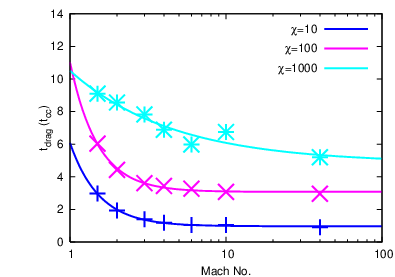
Fig. 15 shows the Mach number and $\chi$ dependence of $t_{\rm drag}$ and $t_{\rm mix}$, two of the important timescales which characterize the evolution and destruction of the cloud. The results of least-squares fits to these plots are noted in Tables 4 and 5. Both $t_{\rm drag}$ and $t_{\rm mix}$ are relatively constant for a given $\chi$ at Mach numbers above 4. This reflects the onset of the “Mach-scaling” mentioned in Section 3. In contrast, $t_{\rm drag}$ and $t_{\rm mix}$ both rise sharply at lower Mach numbers: cloud drag and the mixing of material from the cloud are less efficient with low shock Mach numbers. This is because: i) the density jump across the shock and the speed of the postshock intercloud flow past the cloud are lower when $M$ is smaller; and ii) the growth rate of KH instabilities is slower.

The cloud is accelerated by two processes. First, the shock driven into the cloud accelerates it to a speed $v_{\rm s}$. Further acceleration then occurs as the shocked intercloud gas flows past the cloud, until they have the same velocity. For large $\chi$ the second stage dominates and $v_{\rm s}/v_{\rm b}$ is small. Solving the equation of motion for the cloud (Klein et al. 1994, see, e.g., Eq. 2.5 in) in the strong shock limit for $\gamma=5/3$ gives

where $C_{\rm D}$ is the drag coefficient (Klein et al. 1994, see Section 2.1 of). In the general case we find

For both Eqs. 9 and 10, the cross-sectional area of the cloud is assumed to remain constant. This is a poor approximation which leads to an overestimate of the drag time, since the shock causes the cloud to rapidly expand in the transverse direction (Fig. 5). Nonetheless, it is useful to compare the ratio $t_{\rm drag(g)}/t_{\rm drag(s)}$ with $M$. For $\gamma=5/3$ and $M=1.5$, we find that $t_{\rm drag(g)}/t_{\rm drag(s)}\approx 4$. Comparing to Fig. 15(a) we see that the ratio of $t_{\rm drag}$ when $M=1.5$ to when $M=40$ is 3.3, 2.0, and 1.7 for $\chi=10$, $10^{2}$, and $10^{3}$, respectively. Hence the Mach number dependence of the drag time scales nearly as expected when $\chi=10$. However, the drag time for low values of $M$ is increasingly overestimated compared to the simulations as $\chi$ increases. This divergence is at least partly due to differences in the expansion behaviour of the cloud: comparing simulations m1.5c3 and m10c3, one sees that $a_{\rm cloud}$ is significantly greater in the former until $t\approx 7\,t_{\rm cc}$ (see Fig. 5c).

At face value the fits in Fig. 15(a) to the numerically obtained drag times imply that $C_{\rm D}\approx 5$, 5, and 10 for $\chi=10$, $10^{2}$, and $10^{3}$ respectively. These values are much larger than one expects (the true values of $C_{\rm D}$ are likely to be $\mathrel{\hbox to0.0pt{\lower 3.0pt\hbox{$\sim$}\hss}\raise 2.0pt\hbox{$<$}}1$ - see Landau & Lifshitz 1959, for solid bodies). This difference is again caused by the fact that the cross-sectional area of the cloud does not remain constant.

Fig. 15 also shows that the mixing time of the core, $t_{\rm mix}$, is always greater than the drag time of the cloud, $t_{\rm drag}$. The ratio of $t_{\rm mix}/t_{\rm drag}$ is also dependent on $\chi$, this ratio being greatest at low values of $\chi$, but declining with increasing $\chi$ as the relative efficiency of mixing relative to acceleration increases. For clouds with $\chi=10$, the numerical simulations reveal that $t_{\rm mix}/t_{\rm drag}$ increases from 1.39 at $M=1.5$, peaking at 1.67 at $M=3$, and thereafter declines to 1.56 at $M=40$. When $\chi=10^{3}$, $t_{\rm mix}/t_{\rm drag}$ declines from a value of 1.45 at $M=1.5$, to 1.15 at $M=40$.

The values of $t_{\rm drag}$ and $t_{\rm mix}$ display greater scatter about the least squares fit when $\chi=10^{3}$ compared to the fits at lower values of $\chi$. This is due to large scale RT instabilites in these models which randomly and spontaneously fragment the cloud. The values of $t_{\rm drag}$ and $t_{\rm mix}$ are generally higher in inviscid calculations, and display larger scatter. The extra viscosity that the subgrid turbulence model imposes on the hydrodynamic grid helps suppress some of the random fluctuations during the interaction, and also leads to better convergence in resolution tests (Pittard et al. 2009).

Fig. 16 shows the time evolution of the velocity dispersions, $\delta v_{\rm z}$ and $\delta v_{\rm r}$. Their behaviours are broadly similar for interactions with supersonic post-shock flow ($M=3$ and $M=10$). However, the velocity dispersions in the $M=1.5$ simulations build more slowly, and are limited to lower maximum values, reflecting the weaker interaction. $\delta v_{\rm z}$ peaks at higher values with $\chi$, due to greater growth of KH and RT instabilities resulting from the longer drag and mixing timescales with $\chi$. The ratio $\delta v_{z}/\delta v_{\rm r}$ is not strongly dependent on $M$, in contrast to its variation with $\chi$. The latter point was noted previously by Klein et al. (1994) and Pittard et al. (2009).

The time evolution of the energy in sub-grid turbulent motions is shown in Fig. 13. It rises more rapidly and peaks at higher values in simulations with high Mach numbers and cloud density contrast. When $\chi=10^{3}$, it peaks at about 3 percent in models with $M=3$ and $M=10$, but peaks at only 1 percent when $M=1.5$. In models with $\chi=10$ it peaks at less than 1 per cent, and reaches a maximum value of only 0.2 percent when $M=1.5$. The peak in the sub-grid turbulent energy fraction is relatively narrow when $\chi\mathrel{\hbox to0.0pt{\lower 3.0pt\hbox{$\sim$}\hss}\raise 2.0pt\hbox{$>$}}10^{2}$, with most of the turbulent energy being dissipated by $t=10\;t_{\rm cc}$. In contrast, when $\chi=10$, the sub-grid turbulent energy can be roughly constant for durations in excess of $15\;t_{\rm cc}$.

The velocity dispersions shown in Fig. 16 are global averages over the entire cloud. These can be used to obtain a globally averaged energy fraction of the fluctuations. For model m10c3, $\delta v_{\rm r}$ and $\delta v_{\rm z}$ peak at $t\approx 7.25\,t_{\rm cc}$, with values of $\approx 0.09\,v_{\rm b}$ and $\approx 0.23\,v_{\rm b}$ respectively. Hence, the global velocity dispersion, $\delta v=\sqrt{(2\delta v_{\rm r}^{2}+\delta v_{\rm z}^{2})/3}\approx 0.15\,v_{\rm b}$. This is about twice the value noted by Nakamura et al. (2006) for their simulations of radiative clouds with $\gamma=1.1$. The ratio of the energy in (resolved) fluctuations to the kinetic energy of the mean flow is $(\delta v/v)^{2}\approx 0.2$.

However, such global estimates of $\delta v$ and $(\delta v/v)^{2}$ are actually upper limits. Fig. 17 shows the mean axial velocity, $v_{\rm z}$, and the velocity dispersions $\delta v_{\rm z}$ and $\delta v_{\rm r}$, evaluated on a more local scale. The tiles in these maps are of size $0.5\times 0.5\,r_{\rm c}$, and contain up to 4096 individual cells from the hydrodynamic calculation, over which the displayed quantities are averaged. These averages are again mass-weighted quantities, but consider material only within each tile - i.e. $\delta v_{\rm z}$ is again calculated using Eq. 23 in Paper I, but $\langle v_{\rm z}^{2}\rangle$ and $\langle v_{\rm z}\rangle$ are evaluated only for the material within each tile. Note that $\delta v_{\rm r}$ will be non-zero even when $v_{\rm r}$ is constant over each tile. This is a consequence of the specific averaging formula. The maps in Fig. 17 were calculated at $t=5.66\,t_{\rm cc}$ for clouds with $\chi=10^{3}$ hit by a Mach 1.5 (a) and a Mach 10 (b) shock (for which the corresponding density plots are shown in Fig. 2), and also at $t=7.10\,t_{\rm cc}$ for the $M=10$ case (panel c).

In Fig. 17(a) and (b), the mean axial velocity is highest at the slip surface between cloud and ambient material, and is lowest in the central core of the tail. A velocity gradient perpendicular to the tail is clearly present. Both the $r$ and $z-$components of the velocity dispersion are also greatest at the slip surface. Also shown is ${\rm log_{10}}(\delta v/v)^{2}$, which has a maximum value of $-0.1$ in Fig. 17(a), and $-0.92$ in Fig. 17(b). Slightly later in the m10c3 simulation, a large fragment breaks away from the cloud core. This fragment is responsible for a significant increase in the local and globally averaged velocity dispersions, as seen in Figs. 17(c) and 16, respectively. The peak local value of $(\delta v/v)^{2}=0.6$, indicating that there are regions in the flow where the swirling motions within the gas are almost as fast as its average bulk speed.

Our aim in this section is simply to highlight how the velocity dispersion varies on smaller scales in the flow. This is of interest given that spatial variations in the velocity and the velocity dispersion of clouds and tails can be probed using high-spatial-resolution observations (Meaburn et al. 1998; Meaburn & Boumis 2009, see, e.g.,). We also wished to draw attention to the fact that while the local velocity dispersion may exceed the globally averaged value, the latter is in turn an upper limit for the whole cloud.

References

- Arthur & Henney (1996) Arthur S. J., Henney W. J., 1996, ApJ, 457, 752
- Arthur et al. (1993) Arthur S. J., Dyson J. E., Hartquist T. W., 1993, MNRAS, 261, 425
- Arthur et al. (1996) Arthur S. J., Henney W. J., Dyson J. E., 1996, A&A, 313, 897
- Cecil, Bland-Hawthorn & Veilleux (2002) Cecil G., Bland-Hawthorn J., Veilleux S., 2002, ApJ, 576, 745
- Chièze & Lazareff (1981) Chièze J. P., Lazareff B., 1981, A&A, 95, 194
- Conselice et al. (2001) Conselice C. J., Gallagher J. S., Wyse R. F. G., 2001, ApJ, 122, 2281
- Cooper et al. (2009) Cooper J. L., Bicknell G. V., Sutherland R. S., Bland-Hawthorn J., 2009, ApJ, 703, 330
- Danforth et al. (2001) Danforth C. W., Blair W. P., Raymond J. C., 2001, AJ, 122, 938
- Dash & Wolf (1983) Dash S. M., Wolf D. E., 1983, AIAA paper 83-0704
- Dyson & Hartquist (1987) Dyson J. E., Hartquist T. W., 1987, MNRAS, 228, 453
- Dyson et al. (2002) Dyson J. E., Arthur S. J., Hartquist T. W., 2002, A&A, 390, 1063
- Dyson et al. (2006) Dyson J. E., Pittard J. M., Meaburn J., Falle S. A. E. G., 2006, A&A, 457, 561
- Dyson et al. (1995) Dyson J. E., Williams R. J. R., Redman M. P., 1995, MNRAS, 237, 700
- Falle (1991) Falle S. A. E. G., 1991, MNRAS, 250, 581
- Falle et al. (2002) Falle S. A. E. G., Coker R. F., Pittard J. M., Dyson J. E., Hartquist T. W., 2002, MNRAS, 329, 670
- Fragile et al. (2004) Fragile P. C., Murray S. D., Anninos P., van Breugel W., 2004, ApJ, 604, 74
- García-Arredondo et al. (2002) García-Arredondo F., Arthur S. J., Henney W. J., 2002, RMxAA, 38, 51
- Gregori et al. (2000) Gregori G., Miniati F., Ryu D., Jones T. W., 2000, ApJ, 543, 775
- Hartquist et al. (1986) Hartquist T. W., Dyson J. E., Pettini M., Smith L.J., MNRAS, 1986, 221, 715
- Klein et al. (1994) Klein R. I., McKee C. F., Colella P., 1994, ApJ, 420, 213
- Landau & Lifshitz (1959) Landau L. D., Lifshitz E. M., 1959, in “Fluid Mechanics” (Pergamon Press, Oxford)
- Levenson et al. (2002) Levenson N. A., Graham J. R., Walters J. L., 2002, ApJ, 576, 798
- Mac Low et al. (1994) Mac Low M.-M., McKee C. F., Klein R. I., Stone J. M., Norman M. L., 1994, ApJ, 433, 757
- Marcolini et al. (2005) Marcolini A., Strickland D. K., D’Ercole A., Heckman T. M., Hoopes C. G., 2005, MNRAS, 362, 626
- Martin et al. (2007) Martin D. C., et al., 2007, Nat, 448, 780
- Matsuura et al. (2009) Matsuura M., et al., ApJ, 700, 1067
- McKee & Ostriker (1977) McKee C. F., Ostriker J. P., 1977, ApJ, 218, 148
- Meaburn & Boumis (2009) Meaburn J., & Boumis P., 2009, MNRAS, in press
- Meaburn et al. (1998) Meaburn J., Clayton C. A., Bryce M., Walsh J. R., Holloway A. J., Steffen W., 1998, MNRAS, 294, 201
- Melioli et al. (2005) Melioli C., de Gouveia Dal Pino E. M., Raga A., 2005, A&A, 443, 495
- Mellema, Kurk & Röttgering (2002) Mellema G., Kurk J. D., Röttgering H. J. A., 2002, A&A, 395, L13
- Miesch & Zweibel (1994) Miesch M. S., Zweibel E. G., 1994, ApJ, 432, 622
- Nakamura et al. (2006) Nakamura F., McKee C. F., Klein R. I., Fisher R. T., 2006, ApJSS, 164, 477
- Orlando et al. (2005) Orlando S., Peres G., Reale F., Bocchino F., Rosner R., Plewa T., Siegel A., 2005, A&A, 444, 505
- Orlando et al. (2008) Orlando S., Bocchino F., Reale F., Peres G., Pagano P., 2008, ApJ, accepted (arxiv::0801.1403)
- Patnaude & Fesen (2005) Patnaude D. J., Fesen R. A., 2005, ApJ, 633, 240
- Pittard (2007) Pittard J. M., 2007, in “Diffuse Matter From Star Forming Regions to Active Galaxies” (Springer-Verlag, Heidelberg)
- Pittard et al. (2003b) Pittard J. M., Arthur S. J., Dyson J. E., Falle S. A. E. G., Hartquist T. W., Knight M. I., Pexton M., 2003b, A&A, 401, 1027
- Pittard et al. (2005) Pittard J. M., Dyson J. E., Falle S. A. E. G., Hartquist, 2005, MNRAS, 361, 1077
- Pittard et al. (2009) Pittard J. M., Falle S. A. E. G., Hartquist T. W., Dyson J. E., 2009, MNRAS, 394, 1351
- Pittard et al. (2003a) Pittard J. M., Hartquist T. W., Ashmore I., 2003a, A&A, 408, 813
- Pittard et al. (2001a) Pittard J. M., Hartquist T. W., Dyson J. E., 2001a, A&A, 373, 1043
- Pittard et al. (2004) Pittard J. M., Hartquist T. W., Ashmore I., Byfield A., Dyson J. E., Falle S. A. E. G., 2004, A&A, 414, 399
- Pittard et al. (2001b) Pittard J. M., Dyson J. E., Hartquist T. W., 2001b, A&A, 367, 1000
- Poludnenko et al. (2002) Poludnenko A. Y., Frank A., Blackman E. G., 2002, ApJ, 576, 832
- Poludnenko et al. (2004) Poludnenko A. Y., Frank A., Mitran S., 2004, ApJ, 613, 387
- Pope et al. (2008) Pope E. C. D., Pittard J. M., Hartquist T. W., Falle S. A. E. G., 2008, MNRAS, 385, 1779
- Raga et al. (2007) Raga A. C., Esquivel A., Riera A., Velázquez P. F., 2007, ApJ, 668, 310
- Shin et al. (2008) Shin M.-S., Stone J. M., Snyder G. F., 2008, ApJ, accepted (arXiv:0802.2708)
- Smith (1996) Smith S. J., 1996, ApJ, 473, 773
- Stone & Norman (1992) Stone J. M., Norman M. L., 1992, ApJ, 390, L17
- Strickland & Stevens (2000) Strickland D. K., Stevens I. R., 2000, MNRAS, 314, 511
- Strickland et al. (2000) Strickland D. K., Heckman T. M., Weaver K. A., Dahlem M., 2000, AJ, 120, 2965
- Toniazzo et al. (2001) Toniazzo T., Hartquist T. W., Durisen R. H., 2001, MNRAS, 322, 149
- van Loo et al. (2007) van Loo, S., Falle S. A. E. G., Hartquist T. W., Moore T. J. T., 2007, A&A, 471, 213
- Veilleux et al. (2005) Veilleux S., Cecil G., Bland-Hawthorn J., 2005, ARA&A, 43, 769
- Vieser & Hensler (2007) Vieser W., Hensler G., 2007, A&A, 472, 141
- Weaver et al. (1977) Weaver R., McCray R., Castor J., Shapiro P., Moore R., 1977, ApJ, 218, 377
- Westmoquette et al. (2009) Westmoquette M. S., Gallagher J. S., Smith L. J., Trancho G., Bastian N., Konstantopoulos I. S., 2009, ApJ, accepted (arXiv:0907.3162)
- Westmoquette et al. (2007) Westmoquette M. S., Smith L. J., Gallagher J. S. III, O’Connell R. W., Rosario D. J., De Grijs R., 2007, ApJ, 671, 358
- White & Long (1991) White R. L., Long K. S., 1991, ApJ, 373, 543
- Williams et al. (1999) Williams R. J. R., Dyson J. E., Hartquist T. W., 1999, A&A, 344, 675
- Williams et al. (1995) Williams R. J. R., Hartquist T. W., Dyson J. E., 1995, ApJ, 446, 759