Deformations of bordered Riemann surfaces and associahedral polytopes
Abstract.
We consider the moduli space of bordered Riemann surfaces with boundary and marked points. Such spaces appear in open-closed string theory, particularly with respect to holomorphic curves with Lagrangian submanifolds. We consider a combinatorial framework to view the compactification of this space based on the pair-of-pants decomposition of the surface, relating it to the well-known phenomenon of bubbling. Our main result classifies all such spaces that can be realized as convex polytopes. A new polytope is introduced based on truncations of cubes, and its combinatorial and algebraic structures are related to generalizations of associahedra and multiplihedra.
Key words and phrases:
moduli, compactification, associahedron, multiplihedron2000 Mathematics Subject Classification
14H10, 52B11, 05A191. Overview
The moduli space of Riemann surfaces of genus with marked particles has become a central object in many areas of mathematics and theoretical physics, ranging from operads, to quantum cohomology, to symplectic geometry. This space has a natural extension by considering Riemann surfaces with boundary. Such objects typically appear in open-closed string theory, particularly with respect to holomorphic curves with Lagrangian submanifolds. Although there has been much study of these moduli spaces from an analytic and geometric setting, a combinatorial and topological viewpoint has been lacking. At a high level, this paper can be viewed as an extension of the work by Liu [16] on the moduli of -holomorphic curves and open Gromov-Witten invariants. In particular, Liu gives several examples of moduli spaces of bordered Riemann surfaces, exploring their stratifications. We provide a combinatorial understanding of this stratification and classify all such spaces that can be realized as convex polytopes, relating it to the well-known phenomenon of bubbling.
There are several (overlapping) fields which touch upon ideas in this paper. Similar to our focus on studying bordered surfaces with marked points, recent work spearheaded by Fomin, Shapiro and Thurston [11] has established a world of cluster algebras related to such surfaces. This brings in their notions of triangulated surfaces and tagged arc complexes, whereas our viewpoint focuses on the pair of pants decomposition of these surfaces. Another interest in these ideas come from algebraic and symplectic geometery. Here, an analytic approach can be taken to construct moduli spaces of bordered surfaces and their relationship to Gromov-Witten theory, such as the one by Fukaya and others [12], or an algebraic method can used, like that of Harrelson, Voronov and Zuniga, to formulate a Batalin-Vilkovisky quantum master equation for open-closed string theory [13]. A third field of intersection comes from the world of operads and algebraic structures. Indeed, the natural convex polytopes appearing in our setting fit comfortably in the framework of higher category theory and the study of and structures seen from generalizations of associahedra, cyclohedra and multiplihedra [8].
An overview of the paper is as follows: Section 2 supplies a review of the definitions of the moduli spaces of interest. Section 3 constructs the moduli spaces and provides detailed examples of several low-dimensional cases and their stratifications. The main theorems classifying the polytopal spaces are provided in Section 4 as well as an introduction to the associahedron and cyclohedron polytopes. A new polytope is introduced and constructed in Section 5 based on the moduli space of the annulus. Finally, the combinatorial and algebraic properties of this polytope are explored and related to the multiplihedron in Section 6.
Acknowledgments.
We thank Chiu-Chu Melissa Liu for her enthusiasm, kindness, and patience in explaining her work, along with Ben Fehrman, Stefan Forcey, Jim Stasheff and Aditi Vashista for helpful conversations. We are also grateful to the NSF for partially supporting this work with grant DMS-0353634. The first author also thanks MSRI for their hospitality, support and stimulating atmosphere in Fall 2009 during the Tropical Geometry and Symplectic Topology programs.
2. Definitions
2.1.
We introduce notation and state several definitions as we look at moduli spaces of surfaces with boundary. Although we cover these ideas rather quickly, most of the detailed constructions behind our statements can be found in Abikoff [1], Sepälä [18, Section 3], Katz and Liu [14, Section 3] and Liu [16, Section 4].
A smooth connected oriented bordered Riemann surface of type has genus with disjoint ordered circles for its boundary. We assume the surface is compact whose boundary is equipped with the holomorphic structure induced by a holomorphic atlas on the surface. Specifically, the boundary circles will always be given the orientation induced by the complex structure. The surface has a marking set of type if there are labeled marked points in the interior of (called punctures) and labeled marked points on the boundary component , where . Throughout the paper, we define .
Definition.
The set fulfilling the above requirements is called a marked bordered Riemann surface. We say is stable if its automorphism group is finite.
Figure 1(a) shows an example of where is of type and is of type . Indeed, any stable marked bordered Riemann surface has a unique hyperboic metric such that it is compatible with the complex structure, where all the boundary circles are geodesics, all punctures are cusps, and all boundary marked points are half cusps. We assume all our spaces are stable throughout this paper.

2.2.
The complex double of a bordered Riemann surface is the oriented double cover of without boundary.11 1 The complex double and the Schottky double of a Riemann surface coincide since it is orientable. It is formed by gluing and its mirror image along their boundaries; see [2] for a detailed construction. For example, the disk is the surface of type whose complex double is a sphere, whereas the annulus is the surface of type whose complex double is a torus. Figure 1(b) shows the complex double of from part (a). In the case when has no boundary, the double is simply the trivial disconnected double-cover of .
The pair is called a symmetric Riemann surface, where is the anti-holormorphic involution. The symmetric Riemann surface with a marking set of type has an involution together with distinct interior points such that , along with boundary points such that .
Definition.
A pair of pants is a sphere from which three points or disjoint closed disks have been removed. A pair of pants can be equipped with a unique hyperbolic structure compatible with the complex structure such that the boundary curves are geodesics.
Let be a surface without boundary. A decomposition of into pairs of pants is a collection of disjoint pairs of pant on such that their union covers the entire surface and their pairwise intersection (of their closures) are either empty or a union of marked points and closed geodesic curves on . Indeed, all the marked points of appear as boundary components of pairs of pants in any decomposition of . A disjoint set of curves decomposing the surface into pairs of pants will be realized by a unique set of disjoint geodesics since there is only one geodesic in each homotopy class.
We now extend this decomposition to include marked surfaces with boundary. Consider the complex double of a marked bordered Riemann surface . If is a decomposition of into pairs of pants, then is another decomposition into pairs of pants. The following is a generalization of the work of Seppälä:
Lemma 1.
[16, Section 4] There exists a decomposition of into pairs of pants such that and the decomposing curves are simple closed geodesics of .
Figure 2(a) shows examples of some of the geodesic arcs from a decomposition of , where part (b) shows the corresponding decomposition for . Notice that there are three types of decomposing geodesics .
- (1)
Involution fixes all points on : The geodesic must be a boundary curve of , such as the curve labeled in Figure 2(b).
- (2)
Involution fixes no points on : The geodesic must be a closed curve on , such as the curve labeled in Figure 2(b).
- (3)
Involution fixes two points on : The geodesic must be an arc on , with its endpoints on the boundary of the surface, such as the curve labeled in Figure 2(b).

We assign a weight to each type of decomposing geodesic in a pair of pants decomposition, corresponding to the number of Fenchel-Nielsen coordinates needed to describe the geodesic. The geodesic of type (2) above has weight two because it needs two Fenchel-Nielsen coordinates to describe it (length and twisting angle), whereas geodesics of types (1) and (3) have weight one (needing only their length coordinates). The following is obtained from a result of Abikoff [1, Chapter 2].
Lemma 2.
Every pair of pants decomposition of a marked bordered Riemann surface of type with marking set has a total weight of
| (2.1) |
from the weighted decomposing curves.
2.3.
Based on the discussion above, we can reformulate the decomposing curves on marked bordered Riemann surfaces in a combinatorial setting:
Definition.
An arc is a curve on such that its endpoints are on the boundary of , it does not intersect nor itself, and it cannot be deformed arbitrarily close to a point on or in . An arc corresponds to a geodesic decomposing curve of type (3) above.
Definition.
A loop is an arc whose endpoints are identified. There are two types of loops: A -loop can be deformed to a boundary circle of having no marked points, associated to a decomposing curve of type (1) above. Those belonging to curves of type (2) are called -loops.
We consider isotopy classes of arcs and loops. Two arcs or loops are compatible if there are curves in their respective isotopy classes which do not intersect. The weighting of geodesics based on their Fenchel-Nielsen coordinates now extends to weights assigned to arcs and loops: Every arc and 1-loop has weight one, and a 2-loop has weight two.
Figure 3 provides examples of marked bordered Riemann surfaces (all of genus 0). Parts (a – c) show examples of compatible arcs and loops. Part (d) shows examples of arc and loops that are not allowed. Here, either they are intersecting the marked point set or they are trivial arcs and loops, which can be deformed arbitrarily close to a point on or in . We bring up this distinction to denote the combinatorial difference between our situation and the world of arc complexes, recently highlighted by Fomin, Shapiro, and Thurston [11].

3. The moduli space
3.1.
Given the definition of a marked bordered Riemann surfaces, we are now in position to study its moduli space. For a bordered Riemann surface of type with marking set of type , we denote as its compactified moduli space. Analytic methods can be used for the construction of this moduli space which follow from several important, foundational cases. Indeed, the moduli space is simply the classic Deligne-Mumford-Knudsen space coming from GIT quotients. The topology of the moduli space of algebraic curves of genus with marked points was provided by Abikoff [1]. Later, Seppälä gave a topology for the moduli space of real algebraic curves [18]. Finally, Liu modified this for marked bordered Riemann surfaces; the reader is encouraged to consult [16, Section 4] for a detailed treatment of the construction of .
Theorem 3.
[16] The moduli space of marked bordered Riemann surfaces is equipped with a (Fenchel-Nielson) topology which is Hausdorff. The space is compact and orientable with real dimension
The dimension of this space should be familiar: It is the total weight of the decomposing curves of the surface given in Equation (2.1). Indeed, the stratification of this space is given by collections of compatible arcs and loops (corresponding to decomposing geodesics) on where a collection of geodesics of total weight corresponds to a (real) codimension stratum of the moduli space. The compactification of this space is obtained by the contraction of the arcs and loops — the degeneration of a decomposing geodesic as its length collapses to .
There are four possible results obtained from a contraction; each one of them could be viewed naturally in the complex double setting. The first is the contraction of an arc with endpoints on the same boundary, as shown by an example in Figure 4.

The arc of part (a) becomes a double point on the boundary in (b), being shared by the two surfaces.22 2 We abuse terminology slightly by sometimes refering to these double points as marked points. Similarly, one can have a contraction of an arc with endpoints on two distinct boundary components as pictured in Figure 5. In both these cases, we are allowed to normalize this degeneration by pulling off (and doubling) the nodal singularity, as in Figure 5(c).

The other two possibilities of contraction lie with loops, as displayed in Figure 6. Part (a) shows the contraction of a 1-loop collapsing into a puncture, whereas part (b) gives the contraction of a 2-loop resulting in the classical notion of bubbling.

3.2.
We presents several examples of low-dimensional marked bordered moduli spaces.
Example.
Consider the moduli space of a disk with two punctures. By Theorem 3, the dimension of this space is one. There are only two boundary strata, one with an arc and another with a loop, showing this space to be an interval. Figure 7 displays this example.

The left endpoint is the moduli space of a thrice-punctured sphere, whereas the right endpoint is the product of the moduli spaces of punctured disks with a marked point on the boundary.
Example.
The moduli space can be seen as a topological disk with five boundary strata. It has three vertices and two edges, given in Figure 8, and is two-dimensional due to Theorem 3. Note that the central vertex in this disk shows this space is not a CW-complex. The reason for this comes from the weighting of the geodesics. Since the loop drawn on the surface representing the central vertex has weight two, the codimension of this strata increases by two.

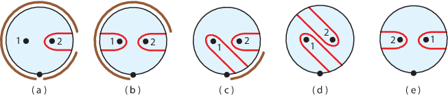
Figure 9 shows why there are two distinct vertices on the boundary of this moduli space. Having drawn one arc cuts the boundary of the disk into two pieces, as labeled in (a). The two ways of adding a second arc, shown in (b) and (c), results in the two vertices. Note that this simply amounts to relabeling the collision of the punctures with the boundary as given by (d) and (e).
Example.
Thus far, we have considered moduli spaces of surfaces with one boundary component. Figure 10 shows an example with two boundary components, the space . Like Figure 8, the space is a topological disk, though with a different stratification of boundary pieces. It too is not a CW-complex, again due to a loop of weight two.

Example.
The moduli space is the pentagon, as pictured in Figure 11. As we will see below, this pentagon can be reinterpreted as the 2D associahedron.

Example.

4. Convex Polytopes
4.1.
From the previous examples, we see some of these moduli spaces are convex polytopes whereas others fail to even be CW-complexes. As we see below, those with polytopal structures are all examples of the associahedron polytope.
Definition.
Let be the poset of all diagonalizations of a convex -sided polygon, ordered such that if is obtained from by adding new noncrossing diagonals. The associahedron is a convex polytope of dimension whose face poset is isomorphic to .
The associahedron was originally defined by Stasheff for use in homotopy theory in connection with associativity properties of -spaces [19]. The vertices of are enumerated by the Catalan numbers and its construction as a polytope was given independently by Haiman (unpublished) and Lee [15].
Proposition 4.
Four associahedra appear as moduli spaces of marked bordered surfaces:
- (1)
is the 0D associahedron .
- (2)
is the 1D associahedron .
- (3)
is the 2D associahedron .
- (4)
is the 3D associahedron .
Proof.

It is natural to ask which other marked bordered moduli spaces are convex polytopes, carrying a rich underlying combinatorial structure similar to the associahedra. In other words, we wish to classify those moduli spaces whose stratifications are identical to the face posets of polytopes. We start with the following result:
Theorem 5.
The following moduli spaces are polytopal.
- (1)
with marked points on the boundary of a disk.
- (2)
with marked points on the boundary of a disk with a puncture.
- (3)
with marked points on one boundary circle of an annulus.
The first two cases will be proven below in Propositions 7 and 8, where they are shown to be the associahedron and cyclohedron respectively, and their surfaces are depicted in Figure 14(a) and (b). We devote a later section to prove the third case in Theorem 14, a new convex polytope called the halohedron, whose surface is given in part (c) of the figure. It turns out that these are the only polytopes appearing as moduli of marked bordered surfaces.

Remark.
Parts (1) and (2) of Theorem 5 can be reinterpreted as types and generalized associahedra of Fomin and Zelevinsky [10]. Therefore, it is tempting to think that this new polytope in part (3) could be the type version. This is, however, not the case, as we see below. In particular, the 3D type generalized associahedron is simply the classical associahedron, whereas the 3D polytope of part (3) is different, as displayed on the right side of Figure 21.
Theorem 6.
Proof.
The overview of the proof is as follows: We find certain moduli spaces which do not have polytopal structures, and then show these moduli spaces appearing as lower dimensional strata to the list above. Since polytopes must have polytopal faces, this will show that none of the spaces on the list are polytopal.
Outside of the spaces in Proposition 4 and Theorem 5, the cases of which result in stable spaces that we must consider are the following:
- (1)
when ;
- (2)
when ;
- (3)
when and some ;
- (4)
when , and both and .
We begin with item (1), when . The simplest case to consider is that of a torus with one puncture. (A torus with no punctures is not stable, with infinite automorphim group, and so cannot be considered.) The moduli space of a torus with one puncture is two-dimensional (from Theorem 3) and has the stratification of a 2-sphere, constructed from a 2-cell and a 0-cell. Thus, any other surface of non-zero genus, regardless of the number of marked points or boundary circles will always have appearing in its boundary strata; Figure 15 shows such a case where this punctured torus appears in the boundary of . This immediately eliminates all cases from being polytopal. For the remaining cases, we need only focus on the case.

Now consider item (2), when . When and , the resulting moduli space is exactly the classical compactified moduli space of punctured Riemann spheres. The strata of this space is well-known, indexed by labeled trees, and is not a polytope. For all other values of , where , the space appears as a boundary strata. As we have shown in Figure 8, this space is not a polytope. Similary, for items (3) and (4), the moduli space appears in all strata, with Figure 10 showing the polytopal failure. ∎
Remark.
An alternate understanding of this result lies in 2-loops. Since each 2-loop has weight two, Lemma 2 and Theorem 3 show that any such loop will increase the codimension of the corresponding strata by two. This automatically disqualifies the stratification from being that of a polytope. Indeed, the cases outlined in Theorem 6 are exactly those which allow 2-loops.
4.2.
We close this section with two well-known results.
Proposition 7.
[6, Section 2] The space of marked points on the boundary of a disk is the associahedron .
Sketch of Proof.
Construct a dual between marked points on the boundary of a disk and an -gon by identifying each marked point to an edge of the polygon, in cyclic order. Then each arc on the disk corresponds to a diagonal of the polygon, and since arcs are compatible, the diagonals are noncrossing. Figure 16 shows an example for the 2D case. ∎

Remark.
The appearance of the associahedron as the moduli space is quite natural. Indeed, if we considered all ordered labelings of the marked points on the boundary of the disk, one would obtain , the real points of the Deligne-Mumford space tiled by associahedra [6].
Figure 17 shows (a) the complex double with marked points on the boundary fixed by involution. Part (b) shows the surface with boundary, whereas (c) considers this space with the natural hyperbolic structure, where the marked points become cusps in the plane.

4.3.
A close kin to the associahedron is the cyclohedron. This polytope originally manifested in the work of Bott and Taubes [4] with respect to knot invariants and later given its name by Stasheff.
Definition.
Let be the poset of all diagonalizations of a convex -sided centrally symmetric polygon, ordered such that if is obtained from by adding new noncrossing diagonals. Here, a diagonal will either mean a pair of centrally symmetric diagonals or a diameter of the polygon. The cyclohedron is a convex polytope of dimension whose face poset is isomorphic to .
Proposition 8.
[7, Section 1] The space of marked points on the boundary of a disk with a puncture is the cyclohedron .
Sketch of Proof.
Construct a dual to the marked points on the boundary of the disk to the symmetric -gon by identifying each marked point to a pair of antipodal edges of the polygon, in cyclic order. Then each arc on the disk corresponds to a pair of symmetric diagonals of the polygon; in particular, the arcs which partition the puncture from the boundary points map to the diameters of the polygon. Since arcs are compatible, the diagonals are noncrossing. Figure 18 shows an example for the 2D case. ∎

Remark.
For associahedra, the moduli space of marked points on the boundary of a disk, any arc must have at least two marked points on either side of the partition in order to maintain stability. For the cyclohedra, however, the puncture in the disk allows us to bypass this condition since a punctured disk with one marked point on the boundary is stable. From the perspective of polytopes, this translates into different stratification of the faces: Whereas each face of is a product of associahedra, resulting in an operad structure, faces of are products of associahedra and cyclohedra, yielding a module over an operad.
5. Graph Associahedra and Truncations of Cubes
5.1.
This section focuses on understanding the polytope arising from the moduli space of marked points on an annulus, as shown in Figure 14(c). However, we wish to place this polytope in a much larger context based on truncations of simplices and cubes. We begin with motivating definitions of graph associahedra; the reader is encouraged to see [5, Section 1] for details.
Definition.
Let be a connected graph. A tube is a set of nodes of whose induced graph is a connected proper subgraph of . Two tubes and may interact on the graph as follows:
- (1)
Tubes are nested if .
- (2)
Tubes intersect if and and .
- (3)
Tubes are adjacent if and is a tube in .
Tubes are compatible if they do not intersect and are not adjacent. A tubing of is a set of tubes of such that every pair of tubes in is compatible.
Theorem 9.
[5, Section 3] For a graph with nodes, the graph associahedron is a simple convex polytope of dimension whose face poset is isomorphic to the set of tubings of , ordered such that if is obtained from by adding tubes.
Corollary 10.
When is a path with nodes, becomes the associahedron . Similarly, when is a cycle with nodes, is the cyclohedron .
Figure 19 shows the 2D examples of these cases of graph associahedra, having underlying graphs as paths and cycles, respectively, with three nodes. Compare with Figures 16 and 18.

There exists a natural construction of graph associahedra from iterated truncations of the simplex: For a graph with nodes, let be the -simplex in which each facet (codimension one face) corresponds to a particular node. Each proper subset of nodes of corresponds to a unique face of , defined by the intersection of the faces associated to those nodes, and the empty set corresponds to the face which is the entire polytope .
Theorem 11.
[5, Section 2] For a graph , truncating faces of which correspond to tubes in increasing order of dimension results in the graph associahedron .
5.2.
We now create a new class of polytope that mirror graph associahedra, except now we are interested in truncations of cubes. We begin with the notion of design tubes.
Definition.
Let be a connected graph. A round tube is a set of nodes of whose induced graph is a connected (and not necessarily proper) subgraph of . A square tube is a single node of . Such tubes are called design tubes of . Two design tubes are compatible if
- (1)
when they are both round, they are not adjacent and do not intersect.
- (2)
otherwise, they are not nested.
A design tubing of is a collection of design tubes of such that every pair of tubes in is compatible.
Figure 20 shows examples of design tubings. Note that unlike ordinary tubes, round tubes do not have to be proper subgraphs of . Based on design tubings, we construct a polytope, not from truncations of simplices but cubes:

For a graph with nodes, we define to be the -cube where each pair of opposite facets correspond to a particular node of . Specifically, one facet in the pair represents that node as a round tube and the other represents it as a square tube. Each subset of nodes of , chosen to be either round or square, corresponds to a unique face of , defined by the intersection of the faces associated to those nodes. The empty set corresponds to the face which is the entire polytope .
Definition.
For a graph , truncate faces of which correspond to round tubes in increasing order of dimension. The resulting polytope is the graph cubeahedron.
Example.
Figure 21 displays the construction of when is a cycle with three nodes. The facets of the -cube are labeled with nodes of , each pair of opposite facets being round or square. The first step is the truncation of the corner vertex labeled with the round tube being the entire graph. Then the three edges labeled by tubes are truncated.

Theorem 12.
For a graph with nodes, the graph cubeahedron is a simple convex polytope of dimension whose face poset is isomorphic to the set of design tubings of , ordered such that if is obtained from by adding tubes.
Proof.
The initial truncation of the vertex of where all round-tubed facets intersect creates an -simplex. The labeling of this simplex is the round tube corresponding to the entire graph . The round-tube labeled -faces of induce a labeling of the -faces of this simplex, which can readily be seen as . Since the graph cubeahedron is obtained by iterated truncation of the faces labeled with round tubes, we see from Theorem 11 that this converts into the graph associahedron . The facets of coming from are in bijection with the design tubes of capturing one vertex. The remaining facets of as well as its face poset structure follow immediately from Theorem 9. ∎
Corollary 13.
Let be a graph with vertices, and let and be the number of facets of and respectively. Then
5.3.
We are now in position to justify the introduction of graph cubeahedra in the context of moduli spaces.
Theorem 14.
Let be a cycle with nodes. The moduli space of marked points on one boundary circle of an annulus is the graph cubeahedron . We denote this special case as and call it the halohedron.
Proof.
There are three kinds of boundary appearing in the moduli space. The loop capturing the unmarked circle of the annulus is in bijection with the round tube of the entire graph, as shown in Figure 22(a).

The arcs capturing marked boundary points correspond to the round tube surrounding nodes of the cycle, displayed in parts (b) and (c). Finally, arcs between the two boundary circles of the annulus are in bijection with associated square tubes of the graph, as in (d). The identification of these poset structures are then immediate. ∎
Figure 23(a) shows the labeling of based on arc and loops on an annulus. By construction of the graph cubeahedron, this pentagon should be viewed as a truncation of the square. The 3D halohedron is depicted on the right side of Figure 21.

Remark.
It is natural to expect these polytopes to appear in facets of other moduli spaces. Figure 24 shows why three pentagons of Figure 12 are actually halohedra in disguise: The arc is contracted to a marked point, which can be doubled and pulled open due to normalization. The resulting surface is the pentagon .

6. Combinatorial and Algebraic Structures
6.1.
We close with examining the graph cubeahedron in more detail, especially in the cases when is a path and a cycle. We have discussed in Sections 4.2 and 4.3 the poset structure of associahedra and cyclohedra in terms of polygons. We now talk about the polygonal version of the halohedron : Consider a convex -sided centrally symmetric polygon with an additional central vertex, as given in Figure 25(a). The three kinds of boundary strata which appear in can be interpreted as adding diagonals to the symmetric polygon. Part (b) shows that a “circle diagonal” can be drawn around the vertex, parts (c) and (d) show how a pair of centrally symmetric diagonals can be used, and a diameter can appear as in part (e).

Due to the central vertex of the symmetric polygon, it is important to distinguish a pair of diameters as in (d) versus one diameter as in (e). Indeed, the pair of diagonals are compatible with the circular diagonal, whereas the diameter is not since they intersect. On the other hand, two diameters are compatible since they are considered not to cross due to the central vertex. Figure 23(b) shows the case of now labeled using polygons, showing the compatibility of the different diagonals. We summarize this below.
Definition.
Let be the poset of all diagonalizations of a convex -sided centrally symmetric polygon with a central vertex, ordered such that if is obtained from by adding new noncrossing diagonals. Here, a diagonal will either mean a circle around the central vertex, a pair of centrally symmetric diagonals or a diameter of the polygon. The halohedron is a convex polytope of dimension whose face poset is isomorphic to .
6.2.
Let us now turn to the case of when is a path:
Proposition 15.
If is a path with nodes, then is the associahedron .
Proof.
Let be a path with nodes. From Corollary 10, the associahedron is the graph associahedron . We therefore show a bijection between design tubings of (a path with nodes) and regular tubings of (a path with nodes), as in Figure 26. Each round tube of maps to its corresponding tube of . Any square tube around the -th node of maps to the tube of surrounding the nodes. This mapping between tubes naturally extends to tubings of and since the round and square tubes of cannot be nested. The bijection follows. ∎

We know from Theorem 11 that associahedra can be obtained by truncations of the simplex. But since is obtained by truncations of cubes, Proposition 15 ensures that associahedra can be obtained this way as well. Such an example is depicted in Figure 27, where the 4D associahedron appears as iterated truncations of the 4-cube.

Proposition 16.
The facets of are
- (1)
one copy of
- (2)
copies of and
- (3)
copies of .
Proof.
Recall there are three kinds of codimension one boundary strata appearing in the moduli space . First, there is the unique loop around the unmarked boundary circle, which Proposition 8 reveals as the cyclohedron . Second, there exist arcs between distinct boundary circles, as show in Figure 28(a). This figure establishes a bijection between this facet and , where is a path with nodes. By Theorem 15 above, such facets are associahedra. There are such associahedra since there are such arcs.

Finally, there exist arcs capturing marked boundary points. Such arcs can be contracted and then normalized, as shown in Figure 4. This leads to a product structure of moduli spaces and , where the +1 in both markings appears from the contracted arc. Proposition 7 and Theorem 14 show this facet to be . When is a cycle with nodes, we see from Corollary 13 that the total number of facets of equals the number of facets of plus . By Corollary 10, is the cyclohedron , known to have facets. ∎
6.3.
From an algebraic perspective, the face poset of the associahedron is isomorphic to the poset of ways to associate objects on an interval. Indeed, the associahedra characterize the structure of weakly associative products. Classical examples of weakly associative product structures are the spaces, topological -spaces with weakly associative multiplication of points. The notion of “weakness” should be understood as “up to homotopy,” where there is a path in the space from to . The cyclic version of this is the cyclohedron , whose face poset is isomorphic to the ways to associate objects on a circle. We establish such an algebraic structure for the halohedron . We begin by looking at the algebraic structure behind another classically known polytope, the multiplihedron.
The multiplihedra polytopes, denoted , were first discovered by Stasheff in [20]. They play a similar role for maps of loop spaces as associahedra play for loop spaces. The multiplihedron is a polytope of dimension whose vertices correspond to ways of associating objects and applying an operation . At a high level, the multiplihedron is based on maps , where neither the range nor the domain is strictly associative. The left side of Figure 29 shows the 2D multiplihedron with its vertices labeled. These polytopes have appeared in numerous areas related to deformation and category theories. Notably, work by Forcey [9] finally proved to be a polytope while giving it a geometric realization.

Recently, Mau and Woodward [17] were able to view the multiplihedra as a compactification of the moduli spaces of quilted disks, interpreted from the perspective of cohomological field theories. Here, a quilted disk is defined as a closed disk with a circle (“quilt”) tangent to a unique point in the boundary, along with certain properties.
Halohedra and the more general graph cubeahedra fit into this larger context. Figure 30 serves as our guide. Part (a) of the figure shows the moduli version of the halohedron. Two of its facets are seen as (b) the cyclohedron and (c) the associahedron. If the interior of the annulus is now colored black, as in Figure 30(d), viewed not as a topological hole but a “quilted circle,” we obtain a cyclic version of the multiplihedron. When an arc is drawn from the quilt to the boundary as in part (e), symbolizing (after contraction) a quilted circle tangent to the boundary, we obtain the quilted disk viewpoint of the multiplihedron of Mau and Woodward.

The multiplihedron is based on maps , where neither the range nor the domain is strictly associative. From this perspective, there are several important quotients of the multiplihedron, as given by the following table.
| Strictly Assocative | path | cycle | general |
|---|---|---|---|
| Both and | cube [3] | cube | cube |
| Only | composihedra [9] | cycle composihedra | graph composihedra |
| Only | associahedra | halohedra | graph cubeahedra |
| Neither nor | multiplihedra [20] | cycle multiplihedra | graph multiplihedra [8] |
The case of associativity of both range and domain is discussed by Boardman and Vogt [3], where the result is shown to be the -dimensional cube. The case of an associative domain is described by Forcey [9], where the new quotient of the multiplihedron is called the composihedron; these polytopes are the shapes of the axioms governing composition in higher enriched category theory. The classical case of a strictly associative range (for letters in a path) was originally described in [20], where Stasheff shows that the multiplihedron becomes the associahedron . The right side of Figure 29 shows the underlying algebraic structure of the 2D associahedron viewed as the graph cubeahedron of a path by Proposition 15.

Figure 31 sketches a bijection between the associahedra (as design tubings of 5 nodes from Figure 26) and associativity/function operations on 6 letters. Recall that the face poset of the cyclohedron is isomorphic to the ways to associate objects cyclically. This is a natural generalization of where its face poset is recognized as the ways of associating objects linearly. Instead, if we interpret in the context of Proposition 15, the same natural cyclic generalization gives us the halohedron . In a broader context, the generalization of the multiplihedron to arbitrary graph is given in [8]. A geometric realization of these objects as well as their combinatorial interplay is provided there as well.
References
- [1] W. Abikoff. The real analytic theory of Teichmüller space, Springer-Verlag, 1980.
- [2] N. Alling and N. Greenleaf. Foundations of the theory of Klein surfaces, Springer-Verlag, 1971.
- [3] J. M. Boardman and R. M. Vogt. Homotopy invariant algebraic structures on topological spaces, Springer-Verlag, 1973.
- [4] R. Bott and C. Taubes. On the self-linking of knots. Journal of Mathematical Physics 35 (1994) 5247-5287.
- [5] M. Carr and S. Devadoss. Coxeter complexes and graph-associahedra, Topology and its Applications 153 (2006) 2155-2168.
- [6] S. Devadoss. Tessellations of moduli spaces and the mosaic operad, in Homotopy Invariant Algebraic Structures, Contemporary Mathematics 239 (1999) 91-114
- [7] S. Devadoss. A space of cyclohedra, Discrete and Computational Geometry 29 (2003) 61-75.
- [8] S. Devadoss and S. Forcey. Marked tubes and the graph multiplihedron, Algebraic and Geometric Topology 8 (2008) 2081-2108.
- [9] S. Forcey. Convex hull realizations of the multiplihedra, Topology and its Applications 156 (2008) 326-347.
- [10] S. Fomin and A. Zelevinsky. -systems and generalized associahedra, Annals of Mathematics 158 (2003) 977-1018.
- [11] S. Fomin, M. Shapiro, D. Thurston. Cluster algebras and triangulated surfaces, Part I: Cluster complexes, Acta Mathematica 201 (2008) 83-146.
- [12] K. Fukaya, Y-G Oh, H. Ohta, K. Ono. Lagrangian intersection Floer theory, American Mathematical Society, 2009.
- [13] E. Harrelson, A. Voronov, J. Zuniga. Open-closed moduli spaces and related algebraic structures, preprint arXiv:0709.3874.
- [14] S. Katz and C.C. Liu. Enumerative Geometry of Stable Maps with Lagrangian Boundary Conditions and Multiple Covers of the Disc, Advances in Theory of Mathematical Physics 5 (2002) 1Ð49.
- [15] C. Lee. The associahedron and triangulations of the -gon, European Journal of Combinatorics 10 (1989) 551-560.
- [16] M. Liu. Moduli of -homomorphic curves with Lagrangian boundary conditions and open Gromov-Witten invariants for an -equivariant pair, preprint arxiv:math.0210257.
- [17] S. Mau and C. Woodward. Geometric realizations of the multiplihedron and its complexification, Compositio Mathematica, to appear.
- [18] M. Seppälä. Moduli spaces of stable real algebraic curves, Ann. Scient. Ec. Norm. Sup. 24 (1991) 519-544.
- [19] J. Stasheff. Homotopy associativity of -spaces, Transactions of the AMS 108 (1963) 275-292.
- [20] J. Stasheff. -spaces from a homotopy point of view, Springer-Verlag, 1970.