Landau-Siegel zeros and zeros of the derivative of the Riemann zeta functionThanks:  Research of the first author supported by the American Institute of Mathematics, and the National Science Foundation. Research of the second author supported by the Korea Research Foundation Grant funded by the Korean Government(MOEHRD, Basic Research Promotion Fund)(KRF-2008-313-C00009).

We illustrate Theorem 1.1 with examples which can help build intuition for why $\lambda^{\prime}=0$ does not imply $\lambda=0$.

Our example involves degree $N$ polynomials with all zeros on the unit circle. In other words, characteristic polynomials of matrices in the unitary group $U(N)$. In these examples. $\lambda>0$ but $\lambda^{\prime}=0$, where $\lambda$ and $\lambda^{\prime}$ refer respectively to the large $N$ limits of the normalized gap between zeros, and the rescaled distance between zeros of the derivative and the unit circle. This is the random matrix analogue of $\lambda$ and $\lambda^{\prime}$ for the zeta function.

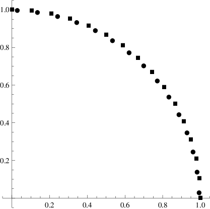
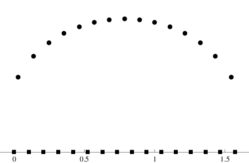
Figure 1.1 illustrates the case of 16 zeros in the interval$\{e^{i\theta}\ :\ 0\leq\theta\leq\pi/2\}$. The plot on the left shows the zeros of the polynomial and its derivative. The figure on the right is the same plot “unrolled”: the horizontal axis is the argument, and the vertical axis is the distance from the unit circle, rescaled by a constant factor.

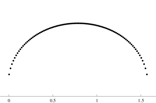
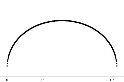
Figure 1.2 is the analogue of the plot on the right side of Figure 1.1, for 101 zeros and 501 zeros. Note that in these examples $\lambda\sim\pi/2$.

In Figure 1.2 the vertical scales are stretched by a factor of $2\pi N(1-r)$ where $N=101$ and $501$, respectively.

Figures 1.1 and 1.2 illustrate that, with this unrolling and rescaling, the zeros of the derivative approach a circle. We see that even though $\lambda>0$ we have $\lambda^{\prime}=0$, but furthermore, since the zeros lie on a (rescaled) circle, we have $m^{\prime}(\nu)\gg\nu^{2}$ as $\nu\to 0$. Thus, we can have $m^{\prime}(\nu)>0$ for all $\nu>0$, yet $m(\nu)=0$ for $\nu$ sufficiently small.

We believe that the above example is the limit of this behavior, and we make the following conjecture, which we view as a refinement of Soundararajan’s conjecture.

We intend this as a general conjecture, applying to the Riemann zeta function but also to other cases such as a sequence of polynomials with all zeros on the unit circle.

For applications to lower bounds of class numbers [10, 1] one does not actually need $m(\nu)>0$ for $\nu<\pi$; it is sufficient to show that a relatively small number of gaps between zeros of the zeta function are small. Our main result, Theorem 1.3, obtains such bounds from estimates on the zeros of the derivative of the zeta function.

Denote $\log_{(2)}t=\log\log t$.

The conclusion of the theorem is weaker than $m(\nu)>0$ for $\nu>0$, but only by a factor of $\log_{(2)}T$. Thus, it is more than sufficient to apply the results of Conrey and Iwaniec [1]. In particular, Theorem 1.3 shows that it is possible to obtain lower bounds for class numbers of imaginary quadratic fields from knowledge of the density of zeros of the derivative of the Riemann zeta function.

There is an apparent discrepancy between Conjecture 1.2 and Theorem 1.3 which we wish to clarify. In Theorem 1.3 we allow exponential decrease of $m^{\prime}(\nu)$ as $\nu\to 0$. While the conclusion of the theorem is weaker than $m(\nu)>0$ by a factor of $\log_{(2)}T$, it may seem curious that the condition in Conjecture 1.2 requires $m^{\prime}(\nu)$ to be relatively large as $\nu\to 0$. Indeed, the examples in Section 1.1 show that the condition in Conjecture 1.2 cannot be improved for general functions.

The reason for the apparent inconsistency is that, as described in Section 2.3, our method relies on a bound on the moments of the logarithmic derivative. For the Riemann zeta function one expects

The bound (1.11) should follow by the method of Selberg [11], although we give a conditional proof that allows us to explicitly determine the implied constant. Such a bound, for one fixed $k$, would establish a weaker version of Theorem 1.3 that required $m^{\prime}(\nu)\gg\nu^{-2k}$. However, more general functions like the polynomials in Section 1.1 do not satisfy an analogous bound to (1.11). In fact, they are very large on the unit circle and do not satisfy the analogue of the Lindelöf hypothesis. Conjecture 1.2 is intended to cover those more general cases, while stronger statements should be true for the zeta function.

It is interesting to speculate on the precise nature of the function $m^{\prime}(\nu)$ for the Riemann zeta function. Dueñez et. al. [2] give a detailed analysis of the relationship between small gaps between zeros of the zeta function (and analogously for zeros of the characteristic polynomial of a random unitary matrix) and the zeros of the derivative which arise from the small gaps. For the case of the Riemann zeta function they indicate that the random matrix conjectures for the zeros of the zeta function should imply

as conjectured by Mezzadri [9]. That calculation is based on a more general result which suggests that if $m(\nu)\sim\kappa\nu^{\beta}$ then $m^{\prime}(\nu)\sim\kappa^{\prime}\nu^{\beta/2}$ where

The factor of $2\pi$ comes from a different normalization used in [2] and here we work with the cumulative distribution functions $m$ and $m^{\prime}$, while in [2] they use density functions. That derivation assumed that zeros of $\zeta^{\prime}$ close to the $\tfrac{1}{2}$-line only arise from closely spaced zeros of the zeta-function. The discussion above shows that, without further knowledge of the zeros, this is not a valid assumption. But, as indicated in our Conjecture 1.2, if $\beta<4$ then we believe that the almost all zeros close to the $\tfrac{1}{2}$-line do arise in such a manner. The random matrix prediction for the neighbor spacing of zeros of the zeta-function has $\kappa=\pi/6$ and $\beta=3$, which is covered by Conjecture 1.2. So our results support the analysis of Dueñez et. al. [2].

The remainder of this paper is devoted to the proof of Theorem 1.3.

We begin the proof of Theorem 1.3. The lemmas in this section show that, in the context of the proof of Theorem 1.3, we only have to deal with zeros that are well spaced.

Suppose, for the purposes of contradiction, that there exists $\epsilon>0$ so that

Then, we can find a sequence $\langle T_{l}\rangle$ such that $T_{1}$ is sufficiently large, $T_{l}\to\infty$ and

as $l\to\infty$. We set

The following lemma shows that we can restrict our attention to those zeros whose immediate neighbors are well spaced.

The next Proposition shows that we can restrict to intervals where the number of zeros is close to its average. Fix $C^{*}>1$, let $l_{1}$ and $l_{2}$ be integers, and for $\tfrac{1}{2}+i\gamma$ a zero of the zeta function set

Using an argument in [5], we get the following.

The proof of Proposition 2.3 is in Section 3.1.

Let $\beta^{\prime}+i\gamma^{\prime}$ be a zero of $\zeta^{\prime}$, and (assuming RH) let $\tfrac{1}{2}+i\gamma_{c}$ be the zero of the zeta function which is closest to $i\gamma^{\prime}$. If there are two closest zeros, choose the one nearer to the origin. We will use the above lemmas to give a lower bound for $M_{\gamma_{c}}$, assuming $\beta^{\prime}-\tfrac{1}{2}$ is small.

Let $Z(T)$ be the set of $\gamma_{c}<T$ which satisfy the following three conditions:

where $s=1/2+1/\log\gamma_{c}+it$ and $|\gamma_{c}-t|\leq A/\log\gamma_{c}$. By the lemmas in the previous section, as $T\to\infty$ the set $Z(T)$ contains $\sim\frac{1}{2\pi}T\log T$ elements. For the remainder of the proof we will assume $\gamma_{c}\in Z(T)$.

Recall Titchmarsh [15], Theorem 9.6(A):

uniformly for $t\geqslant 10$ and $-1\leq\sigma\leq 2$. Let $\beta^{\prime}+i\gamma^{\prime}$ be a zero of $\zeta^{\prime}(s)$ where $0<\gamma^{\prime}<T$ is sufficiently large. Taking the real part (2.18) we have

There are three cases to consider.

Then, by (2.19), we get

Thus, we have $\beta^{\prime}-1/2\gg 1/\log\gamma^{\prime}$.

By (2.19), (2.15), and (2.16), we have

and so again we have

Here the implied constants depend only on $\epsilon$.

Using (2.19), (2.15), and (2.16), as in Case 2, we get

Thus we have

Here the implied constants depend only on $\epsilon$. By (2.25) and the conditions of Case 3 we have

Now take the imaginary part of (2.17) to get

Finally, by (2.15) we have

where

By combining (2.26), (2.27), (2.28), and (2.25), we have

where $1\ll A_{\gamma_{c}}\ll 1$, with the implied constants depending only on $\epsilon$.

Let $\nu$ be a positive number. Suppose that

Then, for sufficiently small $\nu$, we see that only Case 3 is possible for sufficiently large $\gamma^{\prime}$, namely we have

By this, the assumption in Theorem 1.3, and the fact that $\#Z(T)\sim\frac{1}{2\pi}T\log T$, we have

By the last inequality we have

In the next section we describe upper bounds for the moments of $M_{\gamma_{c}}$. This will contradict (2.34) and complete the proof of Theorem 1.3.

We obtain an upper bound on $M_{\gamma_{c}}$ from a bound on moments of the logarithmic derivative of the zeta function. This makes use of that fact that, assuming the zeros of the zeta function do not get close together, the logarithmic derivative can be approximated either by a short sum over zeros, or by a short Dirichlet series.

We assemble the above lemmas to bound the moments of $M_{\gamma_{c}}$.

By Lemma 2.4 and Lemma 2.5, with $A=A_{\epsilon}$ a constant depending only on $\epsilon$, which may be different in each inequality, we have

where $x=T^{1/100k}$, for $|t-\gamma^{\prime}|\leq\delta(\epsilon)/\log\gamma^{\prime}$, provided $\gamma_{c}$ satisfies (2.15) – (2.17). That is, provided $\gamma_{c}\in Z(T)$.

Integrating inequality (2.44) over the set

and then using Lemma 2.6 we get

References

• [1] J.B. Conrey and H. Iwaniec, Spacing of zeros of Hecke LL-functions and the class number problem, Acta Arith. 103 (2002) no. 3, 259-312.
• [2] E. Dueñez, D.W. Farmer, S. Froehlich, C. P. Hughes, F. Mezzadri, and T. Phan, Roots of the derivative of the Riemann zeta function and of characteristic polynomials, preprint.
• [3] D.W. Farmer and R. Rhoades, Differentiation evens out zero spacing, Trans. Amer. Math. Soc., Vol 37, No. 9, 2005, p3789-3811. arXiv:math.NT/0310252
• [4] M.Z. Garaev and C.Y. Yıldırım, On small distances between ordinates of zeros of ζ⁡(s)\zeta(s) and ζ′​(s)\zeta^{\prime}(s), Int. Math. Res. Notices 2007 (2007) Art. ID rnm091, 14 pp.
• [5] A. Ivıć, On small values of the Riemann zeta-function on the critical line and gaps between zeros, Lietuvos Mat. Rinkinys 42 (2002), 31-45
• [6] H. Ki, The zeros of the derivative of the Riemann zeta function near the critical line, Int Math Res Notices (2008) Vol. 2008, Art. ID rnn064, 23 pp. arXiv:0701726
• [7] Levinson N. More than one third of zeros of Riemann’s zeta function are on σ=1/2\sigma=1/2, Adv. Math. 13, 383–436 (1974).
• [8] N. Levinson and H. Montgomery, Zeros of the derivatives of the Riemann zeta-function, Acta Math. 133 (1974), 49-65.
• [9] Mezzadri F. Random matrix theory and the zeros of ζ′​(s)\zeta^{\prime}(s). J. Phys. A: Math. Gen. 36, 2945–2962 (2003).
• [10] H. Montgomery, The pair correlation of zeros of the zeta function, Proc. Sympos. Pure Math. 24, Amer. Math. Soc., Providence, R. I. (1973), 181–193.
• [11] A. Selberg, On the normal density of primes in small intervals,and the difference between consecutive primes, Arch. Math. Naturvid. 47, No. 6 (1943), 87–105.
• [12] Soundararajan, The horizontal distribution of zeros of ζ′​(s)\zeta^{\prime}(s), Duke Math. J. (1998) 91, no 1, 33-59.
• [13] Soundararajan, Moments of the Riemann zeta-function, 11 pp., to appear in Annals of Math. arXiv:0612106.
• [14] Speiser A. Geometrisches zur Riemannschen Zetafunktion, Math. Ann. 110 514–21 (1934).
• [15] E. C. Titchmarsh, The Theory of the Riemann Zeta-function, 2nd ed., revised by D. R. Heath-Brown, Oxford University Press, Oxford, 1986
• [16] K.-M. Tsang, Some Ω\Omega-theorems for the Riemann zeta-function, Acta Arith. 46 (1986), 369–395
• [17] Y. Zhang, On the zeros of ζ′​(s)\zeta^{\prime}(s) near the critical line, Duke Math. J. (2001) 110, No. 3 555-572.