QUARK–DIQUARK SYSTEMATICS OF BARYONS AND THE SYMMETRY FOR LIGHT STATES
Abstract
We continue our attempts to systematize baryons, which are composed of light quarks (), as quark–diquark systems. The notion of two diquarks is used: (i) , with the spin and isospin and (ii) , with and . Here we try to resolve the problem of the low-lying states: in the last experiments the lightest state is observed at MeV, not at MeV as it has been stated 20 years ago. We are looking for different systematization variants with the forbidden low-lying states in the mass region MeV. We see that the inclusion of the constraints on states with angular momentum results in a shift of the lightest isobar to MeV. The scheme with the constraints for low-lying and states (with ) is presented in detail here.
PACS
PACS numbers: 11.25.Hf, 123.1K1 Introduction
Baryons (we mean standard non-exotic baryons) are composite systems of three constituent quarks, each of them in their turn being a complicated system of quarks and gluons. We do not know the detailed structure of baryons, even in the language of constituent quarks, except for a fragmentary knowledge on low-lying states.
We know that low-lying baryons satisfy the symmetry, but as to heavier ones we are not certain about. Numerous model calculations, which describe rather well the low-lying states, are at variance in their predictions concerning highly excited states, e.g., see [1, 2, 3, 4, 5] and references therein. In addition, the number of highly excited states predicted by such models exceeds considerably the number of observed states. One might believe that experimental investigations of baryon spectra were not complete. Nevertheless, it does not remove the question whether it is possible to construct a more effective scheme for highly excited states, with less degrees of freedom and less number of highly excited states. The introduction of another effective particle, that is the diquark, provides us with such a possibility.
The size of diquark as a composite quark–antiquark system is believed to be of the order of that of quark, 0.2–0.3 fm [6, 7]. So, it is doubtful if we can interpret the low–lying baryon (a compact system, 0.7-0.9 fm) as a system of effective diquark and constituent quark.
The idea of baryon as spatially separated quark and diquark can be for sure tried on the highly excited baryon systems which are of a larger size – such an idea was suggested in [8]. But in [8] we accepted also that the quark–diquark structure does not work for low-lying baryons with angular momentum – for these states the symmetry was applied.
Actually, in [8] we have made an attempt to systematize highly excited baryons, assuming that they do not like to be formed as three-particle colour quark systems but prefer to be created as two-particle, quark–diquark, compound states: where is a totally antisymmetrical tensor in the colour space.
In [8] we have considered two schemes of the
quark-diquark construction for the states, namely:
(1) The
diquark masses .
(2) The diquark masses are
equal to each other ; besides, the states
and with the total spin (here
) overlap. This scheme
decreases essentially the number of highly excited states.
In the quark–diquark scheme of [8] we face a specific transition to the limit. This procedure is in fact a projection of the and wave functions on the basis – the result depends on the hypothesis on diquark masses. In the states, at , we have two basic () states, and , see equation (46) in [8], while at the additional basic state, , appears (see equation (49) in [8]).
In the present paper we accept the equality of masses of scalar and axial–vector diquarks, . In recent analyses of spectra near the Roper resonance one may find arguments in favour of the existence of one pole in the partial wave near 1400 MeV. Analytical properties of the partial wave in the best fit of [9, 10] are shown in Fig. 1; the fitting to two poles near 1400 MeV gives us a worse description of data. Of course, the Roper pole splits, owing to the momentum-dependence of width near the branching point. This splitting is quite similar to that observed in the Flatté formula [11] for near the threshold. Still, we attribute such ”satellite poles” to the main one, in case in question, to the Roper pole (); note that in Fig. 1 the satellite pole is hidden under the cut.

There is a question to what low-lying states the symmetry may be applied and where we have the region with spatially separated quark and diquark. Only the experiment can answer this question. If we turn to the PDG compilation [12], it may seem that the symmetry can be applied to only, while at the domain of quark–diquark structures begin. However, the latest analyses [9, 10, 13] give rise to doubts. The matter is that in the experiments carried out in the eighties [14, 15, 16] the resonance has been observed rather definitely. Still, modern analyses [9, 10, 13] point to the lower state, being located around 2200 MeV or even higher. It gives arguments for expanding the symmetry constraints on the states.
In the present paper we accept that both sets of states ( and ) satisfy the symmetry requirements.
The paper is organized as follows:
In Section 2 we present wave functions of quark–diquark states and
demonstrate how the imposing of the constraints affect these systems. In
Section 3 we suggest the setting of the and states, while
states with are discussed in Section 4. Here we demonstrate the setting of all
quark–diquark states on the () and
() trajectories.
2 Wave functions of quark–diquark systems and the constraints
We present here the diquark wave function, give general form for the quark–diquark wave function and present the scheme of projecting them on the basis.
2.1 -wave diquarks and baryons
Recall that we use two -wave diquarks with color numbers : scalar diquark and axial–vector one, . The diquark spin–flavor wave functions with and with read as follows:
| (1) |
Let us consider, first, the isobar at with fixed , total spin and orbital momentum . The wave function for this state at arbitrary reads
| (2) |
Here and are the momenta and momentum angles of the first quark in the c.m. system.
For other , one should include into the wave function a summing over isotopic states which means the following substitution in (2):
| (3) |
To project the wave functions (2) or (3) on the wave function set, we should use symmetrical coordinate/momentum wave functions
| (4) |
For example, one may accept that depends on only, . Indeed, in this limit we have
| (5) |
For nucleon states we write
| (6) |
The limit, as previously, is reached at . Then, instead of (6), one has
| (7) |
For states the wave function reads in general case as follows:
| (8) |
In the limit we have
| (9) |
Baryons are characterized by and , these states with different and and fixed and can mix. To select independent states, one may orthogonalize wave functions with the same isospin and . The orthogonalization depends on the structure of the momentum/coordinate parts . But in case of the limit the momentum/coordinate wave functions transform in the common factor or , and one should orthogonalize the spin/momentum factors. Namely, let us denote the spin/momentum factor of the wave function as . Then
| (10) |
where belong to different . The orthogonal set of operators is constructed in a standard way:
| (11) |
and so on. The convolution of operators includes the summation over quark spins as well as integration over quark momenta.
2.2 Wave functions in the limit
We present wave functions of the and systems in the limit, assuming . The transition gives us additional reduction of number of states.
Recall that in the limit the momentum/coordinate factors of wave functions, for example, such as and , transform into -dependent ones:
| (12) | |||
For our purpose, that is, for checking the number of non-vanishing states, we calculate below the wave functions with and only.
3 Wave functions of the () states in the limit and
In this sector we have only seven basic states, namely,
(1) two with :
,
,
(2) three with : ,
,
,
(3) two with : , .
Below the wave functions are written in c.m. system using the following notations for quark momenta: , .
(1) Two systems with
We have two basic states:
| (13) | |||||
and
| (14) | |||||
The same angular momentum/spin wave functions can be constructed with use of the system, in this way we have two nucleons with :
| (15) | |||||
and
| (16) | |||||
The wave function of (13) coincides with that of (15), while the wave function of (14) coincides with (16), because we use equation (12): . In this case we deal with two (not four) states.
(2) Three systems with
There are three states with :
| (17) | |||||
| (18) | |||||
and
| (19) | |||||
(3) Two states with
In the () sector of states, there are two baryons only in the limit – the states with :
| (20) | |||||
and
| (21) | |||||
3.1 The vanishing class of () states
In the limit, the states with (i.e. , , ) are absent. It is easy to be certain of that, after calculating wave functions with . Indeed,
| (22) |
The absence of , which, being in the set, should be located at MeV, is a primary motivation for expanding the symmetry onto states.
4 The symmetry and the and states
First, we recall the setting of states, then we discuss the situation with states under the symmetry.
4.1 The symmetry for the nucleon , isobar and their radial excitations
We accept and suppose the symmetry for the lowest baryons with . It gives us two ground states – the nucleon and isobar as well as their radial excitations:
|
(23) |
Note that the mass-squared splitting of the nucleon radial excitation states, , is of the order of GeV2. This value is close to that observed in meson sector [7, 17]:
| (24) |
The state with cannot be unambiguously determined.
One can see that the mass-squared splitting of isobars, , coincides with that of the nucleon, , with a good accuracy:
| (25) |
Let us emphasize that state is classified as states, with (see Section 4). However, this resonance can be reliably classified as radial excitations of , with . Actually, it means that around MeV one may expect the double-pole structure.
4.2 Setting of the states under the symmetry constraints
|
|
(26) |
|
|
(27) |
5 The setting of states with
For a ”naive observer”, who does not perform an analysis of double pole structure, the number of states with decreases twice.
In Fig. 2, following [9, 10, 18, 12], we show plots as they look like for naive observers, while Fig. 3 demonstrates the plot for ground states () only.
We have three groups of states with :
| (28) | |||||
and two with :
| (29) | |||||
We suppose that in sector the states of groups (1) and (2) with the same and have the equal masses – resonances are overlapping:
| (30) | |||
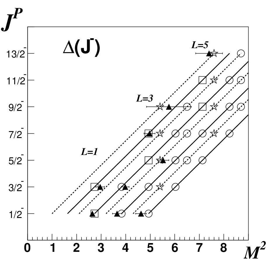


For states the values of baryon masses in the sector are as follows:
|
|
(31) |
and for negative-parity states:
|
|
(32) |
In the sector we have for states:
|
|
(33) |
and for ones:
|
|
(34) |
The above-written equations allow us to predict the plots which are shown in Fig. 4.


6 Conclusion
Under the hypothesis of the quark–diquark structure of highly excited baryons, we succeeded to suggest for them a realistic classification. The introduction of diquarks gave a considerable reduction of excited states; additional reduction was obtained owing to the assumption of the overlapping of states with .
Thus obtained a classification gave linear trajectories in the and planes, which are strictly ordered. There is a number of overlapping poles. The observation of two-pole and three-pole structures in the complex- planes of partial amplitudes is a top-priority task at the analysis of baryon spectra, while the next task consists in the writing and solving the spectral integral equation for quark–diquark systems. Such an equation should be similar to that written and solved before for the system [19].
Acknowledgments
We thank L.G. Dakhno for helpful discussions. The paper was supported by the RFFI grants 07-02-01196-a and RSGSS-3628.2008.2.
References
- [1] N. Izgur and G. Karl, Phys. Rev. D18, 4187 (1978).
- [2] N. Izgur and G. Karl, Phys. Rev. D19, 2653 (1979).
- [3] S. Capstik, N. Izgur, Phys. Rev. D34, 2809 (1986).
- [4] L.Y. Glozman et al., Phys. Rev. D58:094030 (1998).
- [5] U. Löring, B.C. Metsch, H.R. Petry, Eur.Phys. A10, 395 (2001); A10, 447 (2001).
- [6] V.V. Anisovich, M.N. Kobrinsky, J. Nyiri, Yu.M. Shabelski Quark Model and High Energy Collisions , Second Edition, World Scientific, Singapore, 2004.
- [7] A.V. Anisovich, V.V. Anisovich, J. Nyiri, V.A. Nikonov, M.A. Matveev and A.V. Sarantsev, Mesons and Baryons. Systematization and Methods of Analysis, World Scientific, Singapore, 2008.
- [8] A.V. Anisovich, V.V. Anisovich,M.A. Matveev, V.A. Nikonov, A.V. Sarantsev and T.O. Vulfs Searching for the quark-diquark systematics of baryons. Systems composed by the light quarks , arXiv:1001.1259 [hep-ph].
- [9] A.V. Sarantsev, Methods of Data Analysis: Mesons and Baryons, Talk given at the HADRON 2009, XIII Int. Conference on Hadron Spectroscopy, Tallahasee, 2009.
- [10] A.V. Anisovich, Status of the Bonn-Gatchina partial wave analysis, Talk given at the HADRON 2009, XIII Int. Conference on Hadron Spectroscopy, Tallahasee, 2009.
- [11] S.M. Flattë, Phys. Lett. B 63 224 (1974).
- [12] C. Amsler et al. [Particle Data Group], Phys. Lett. B 667 (2008) 1.
- [13] R. A. Arndt, W. J. Briscoe, I. I. Strakovsky and R. L. Workman, Phys. Rev. C 74, 045205 (2006) [arXiv:nucl-th/0605082].
- [14] R. E. Cutkosky, C. P. Forsyth, J. B. Babcock, R. L. Kelly and R. E. Hendrick,
- [15] D. M. Manley and E. M. Saleski, Phys. Rev. D 45, 4002 (1992).
- [16] G. Hohler, In *Bratislava 1973, Proceedings, Triangle Meeting On Hadron Interactions At Low Energies*, Bratislava 1975, 11-75 and Preprint - HOEHLER G (73,REC.DEC) 60p
- [17] A.V. Anisovich, V.V. Anisovich, and A.V. Sarantsev, Phys. Rev. D 62:051502(R) (2000).
- [18] E. Klempt, Baryon Spectroscopy and the Origin of Mass, Talk given at the HADRON 2009, XIII Int. Conference on Hadron Spectroscopy, Tallahasee, 2009.
- [19] V.V. Anisovich, L.G. Dakhno, M.A. Matveev, V.A. Nikonov, and A. V. Sarantsev, Yad. Fiz. 70, 480 (2007) [Phys. Atom. Nucl. 70, 450 (2007)].