Evolution equation for the -meson distribution amplitude
in the heavy-quark effective theory in coordinate space
Abstract
The -meson distribution amplitude (DA) is defined as the matrix element of a quark-antiquark bilocal light-cone operator in the heavy-quark effective theory, corresponding to a long-distance component in the factorization formula for exclusive -meson decays. The evolution equation for the -meson DA is governed by the cusp anomalous dimension as well as the Dokshitzer-Gribov-Lipatov-Altarelli-Parisi-type anomalous dimension, and these anomalous dimensions give the “quasilocal” kernel in the coordinate-space representation. We show that this evolution equation can be solved analytically in the coordinate-space, accomplishing the relevant Sudakov resummation at the next-to-leading logarithmic accuracy. The quasilocal nature leads to a quite simple form of our solution which determines the -meson DA with a quark-antiquark light-cone separation in terms of the DA at a lower renormalization scale with smaller interquark separations (). This formula allows us to present rigorous calculation of the -meson DA at the factorization scale for less than GeV-1, using the recently obtained operator product expansion of the DA as the input at GeV. We also derive the master formula, which reexpresses the integrals of the DA at for the factorization formula by the compact integrals of the DA at GeV.
pacs
12.38.Cy, 12.39.Hg, 12.39.St, 13.25.HwI Introduction
The -meson light-cone distribution amplitude (LCDA) is one of the important ingredients of the QCD factorization formula for exclusive decays [1, 2, 3] and has recently attracted much attention due to its central role for the analysis of the experimental data, e.g., hadronic and radiative -decay data [4]. The -meson LCDA appears in the factorization formula for hard spectator interaction amplitudes, where a large momentum is transferred to the spectator light-quark via gluon exchange [1, 2, 3, 4, 5, 6, 7, 8, 9, 10], and represents the nonperturbative matrix element that describes the leading amplitude to have the valence quark and antiquark with a light-like separation inside the meson [11]. Grozin and Neubert [12] studied constraints on the -meson LCDA from the equations of motion, heavy-quark symmetry and the renormalization group (RG), and they gave the first quantitative estimate of the LCDA using QCD sum rules with the leading perturbative and nonperturbative effects taken into account. The light-cone QCD sum rules for the -decay form factors were also used [13, 14] to estimate the first inverse moment [15] of the LCDA, which participates in the corresponding factorization formula. The Grozin-Neubert’s QCD sum rule calculation was extended by Braun, Ivanov and Korchemsky [16] including the perturbative and nonperturbative corrections, and the importance of the NLO perturbative corrections was emphasized. Indeed, the true non-analytic behavior of the -meson LCDA associated with the “cusp singularities” [17] is only revealed at this level including the radiative corrections [18], and it is this behavior that renders the (non-negative) moments of the LCDA divergent, even after renormalization [12] (see [19] for a similar behavior in three-quark LCDAs for the baryon). Introducing the regularization for the moments with an additional momentum cutoff, Lee and Neubert [20] evaluated the first two moments for a large value of the cutoff in terms of the operator product expansion (OPE) with the NLO perturbative corrections, as well as the power corrections which are generated by the local operators of dimension 4, and they used the results as constrains on model building of the -meson LCDA.
Another feature peculiar to the -meson LCDA is that it involves a complicated mixture of the multiparticle Fock states of higher-twist nature through nonperturbative quark-gluon interactions, as demonstrated using the equations of motion and heavy-quark symmetry [12, 21, 22]. A first systematic treatment of the mixing of the multiparticle states, disentangling the singularities from the radiative corrections, has recently been accomplished by the present authors, and the -meson LCDA is obtained in a form of the OPE as the short-distance expansion for the quark-antiquark light-cone separation, with the subleading and subsubleading power corrections, generated by the local operators of dimension and 5, respectively, and the NLO corrections for the corresponding Wilson coefficients [23]. This OPE enables us to evaluate the -meson LCDA for interquark distances with , where is the renormalization scale of the LCDA, in a rigorous way in terms of three nonperturbative parameters in the heavy-quark effective theory (HQET), one of which is the usual mass difference between the -meson and -quark, , associated with matrix elements of dimension-4 operators, and the other two are the novel HQET parameters [12, 21, 22] associated with matrix elements of the quark-antiquark-gluon three-body operators of dimension 5. Note that the range of where the OPE is directly applicable becomes wider for the smaller value of the scale , as : choosing GeV, corresponding to typical hadronic scale, the model-independent result for interquark distances GeV-1 has been obtained from the OPE and this result has also been used to constrain the behavior of the LCDA at large distances GeV-1 [23]. Those results of the -meson LCDA at GeV have to be evolved to the factorization scale of order that corresponds to the characteristic “hard-collinear” scale for hard spectator scattering in exclusive decays [1, 2, 3], when we substitute the LCDA into the relevant factorization formula.
For this purpose, in principle, we can utilize the analytic solution for the evolution equation of the -meson LCDA obtained in [18, 20]. However, the corresponding solution is directly applicable when the LCDA is given in the momentum representation, which we find inconvenient in our case: the Fourier transformation of the above OPE-based results to the momentum space mixes up the model-independent behavior for GeV-1 with the behavior for GeV-1 which relies on a certain model for the large behavior. On the other hand, it has been noted that the relevant evolution kernel embodies the particularly simple geometrical structure in the coordinate-space representation [16]. These facts motivate us to treat the evolution of the -meson LCDA in an unconventional way, working in the coordinate-space representation. We are able to find the analytic solution for the corresponding evolution equation, and demonstrate that the solution determines the -meson LCDA in terms of the LCDA at a lower scale with smaller interquark separations and thus preserves the boundary at GeV-1 between the model-independent and -dependent behaviors of our LCDA, even after evolving from GeV to . We emphasize that such simple RG structure of the -meson LCDA can be manifested only in the coordinate space. Furthermore, as we shall demonstrate, it is this simple structure that enables us to derive the master formula, by which the relevant integrals of the LCDA at the scale , arising in the factorization formula for the exclusive -meson decays, can be reexpressed by the compact integrals of the LCDA at the scale GeV. Therefore, we believe that the coordinate-space approach for the RG evolution of the -meson LCDA deserves detailed discussions in the present paper. We also show that our solution can be organized so as to include the Sudakov resummation to the next-to-leading logarithmic (NLL) accuracy, taking into account the effects of the anomalous dimension at the two-loop level which is associated with the cusp singularity. We present the first rigorous result of the -meson LCDA at the relevant factorization scale for GeV-1. Combining with the results for the long-distance behavior, we discuss an estimate for the inverse moments of the LCDA at .
The paper is organized as follows. Sec. II is mainly introductory; we give the operator definition of the -meson LCDA, explain the result for its renormalization in the coordinate space, and derive the corresponding RG evolution equation. We demonstrate in Sec. III that, as the solution of this equation, we can obtain the new coordinate-space representation for the evolution of the -meson LCDA, which manifests the simple RG structure, and also organize the result so as to include the Sudakov resummation at the NLL-level. In Sec. IV, we use our coordinate-space representation of the evolution to derive a compact and closed formula for the inverse moments of the LCDA in terms of the certain integrals of the LCDA at a lower scale . Application of our results to calculate the evolution of the OPE-based form of the -meson LCDA is presented in Sec. V, and we discuss an estimate for the inverse moments of the LCDA. Sec. VI is reserved for conclusions.
II Definition and renormalization in the coordinate space
The leading quark-antiquark component of the -meson LCDA is defined as the vacuum-to-meson matrix element in the HQET [12]:
| (1) |
where is the light-antiquark field, is the effective heavy-quark field, and these fields form a gauge-invariant bilocal operator linked by a light-like Wilson line,
| (2) |
with as the light-like vector, and , and denoting the 4-velocity of the meson. The bilocal operator is renormalized at the scale and, here and below, refers to the renormalization scale. In the definition (1),
| (3) |
denotes the -meson decay constant in the HQET [24] and in the RHS is the LCDA in the momentum representation where denotes the light-cone “”-component of the momentum carried by the light antiquark.
The renormalization of the bilocal operator of (1) was studied in [12, 18], calculating the UV divergence in the one-loop diagrams of Fig. 1 in the momentum space (see also [25, 26]). The calculation of those diagrams has also been carried out in the coordinate space [16, 23], and the result yields the renormalization of the bilocal operator in the coordinate-space representation as (unless otherwise indicated, )
| (4) | |||||
connecting the bare and renormalized operators by the “-dependent” renormalization constant in dimensions and Feynman gauge, where , and
| (5) |
with the Euler constant and the “” prescription coming from the position of the pole in the relevant propagators in the coordinate space. The plus-distribution is defined, as usual, as
| (6) |
for a smooth test function . In the one-loop contributions in (4), the first two terms, the double-pole term and the single-pole term involving , manifest the cusp singularity [17] in Fig. 1 (a), i.e., the singularity in the radiative correction around the cusp (at the origin) in the Wilson line,
| (7) |
which is contained in (1), using the relation . The last term in (4) comes from Fig. 1 (b), accompanying the plus-distribution characteristic of the loop integral associated with the massless degrees of freedom only, while the remaining one-loop term comes from the contribution of the renormalization constants of the two quark fields, and . We note that Fig. 1 (c) is UV-finite in the Feynman gauge [27] and does not contribute to (4).

The RG invariance to the one-loop accuracy based on (4) implies that the -meson LCDA (1) obeys the evolution equation in the coordinate space,
| (8) |
with the one-loop RG functions
| (9) | |||||
| (10) |
and
| (11) |
Here, corresponds to the anomalous dimension of the Wilson line with a cusp, (7), and coincides with the LO term of the universal cusp anomalous dimension of Wilson loops with light-like segments [17]; we obtain the finite result (9), because the contribution from the double-pole term of (4) is canceled by the contribution generated by taking the derivative of in the next term with respect to . of (10) represents the anomalous dimension from the above-mentioned contribution of the renormalization constants of the two quark fields, combined with the so-called hybrid anomalous dimension of heavy-light currents in the HQET [24], which governs the scale dependence of the decay constant (3) as, at one-loop accuracy,
| (12) |
of (11) comes from the last term of (4) and represents the -dependent anomalous dimension associated with the massless degrees of freedom only. We note the remarkable property in (8) that the evolution kernel in the RHS, composed of (9)-(11), is quasilocal, such that the evolution mixes the LCDA with itself and with the LCDA associated with smaller light-cone separation (). This is due to the similar structure appearing in the renormalization in the coordinate space, (4), and reflects [16] the fact that the cusp renormalization induced by Fig. 1 (a) is multiplicative in the coordinate space [17] while Fig. 1 (b) gives the contribution identical to the similar correction to the light-quark-antiquark bilocal operators, which embodies simple geometrical structure in the coordinate space so as to mix operators associated with smaller “size” [28].
It is straightforward to perform the Fourier transformation of (8) to the momentum space and derive the evolution equation for of (1), using
| (13) | |||||
and
| (14) | |||||
and, indeed, the result reproduces the evolution equation obtained through the renormalization of the bilocal operator of (1) in the momentum space [18, 25, 26]. We note that the momentum representation of the kernel in (14) coincides with (a part of) the Brodsky-Lepage kernel for the pion LCDA [29] and physically represents a Dokshitzer-Gribov-Lipatov-Altarelli-Parisi (DGLAP) splitting function that vanishes for . On the other hand, a local contribution in (8), associated with the cusp anomalous dimension , yields the new evolution kernel for in the RHS of (13), so that the evolution in the momentum space mixes the LCDA with over the entire region, [18, 25, 20]. We also note that we cannot derive the moment-space representation of the evolution equation (8) in a usual way as in the case of the LCDAs for the light mesons [30], because the presence of the logarithm (5) prevents us from performing the Taylor expansion of (8) about ; indeed, (4) shows that the renormalized LCDA is non-analytic at (see also the discussion in [16, 23]). Thus, the evolution equation for the -meson LCDA manifests simple geometrical structure as the quasilocality of the kernel only in the coordinate-space representation (8).
One may anticipate that the evolution equation (8) would hold to all orders in perturbation theory by taking into account the higher-loop terms in the RG functions (9)-(11). This is correct, at least, for a particular class of higher-loop corrections associated with the universal cusp anomalous dimension of Wilson loops. For example, when we take into account the diagrams that correspond to the two-loop corrections to the relevant Wilson line (7), of (9) gets modified into [17]
| (15) |
with [31]
| (16) |
where and denotes the number of active flavors. Actually, it is not known at present whether the effects of all the other two-loop corrections to the bilocal operator in (1) can be absorbed into the remaining two RG functions in (8), and , as their two-loop terms. Still, the evolution equation (8), with (10), (11) and the two-loop cusp anomalous dimension (15) taken into account, is useful for resumming the Sudakov logarithms to a consistent accuracy, as we will demonstrate in the next section.
III Analytic solution in the coordinate space
The LO solution for the evolution equation of the -meson LCDA was obtained in the momentum representation in [18], and the result determines of (1) as the convolution of at a lower scale and the (complicated) evolution operator, over the entire range of (see (79) in Appendix A). Its Fourier transformation in principle gives the solution for our evolution equation, (8)-(11), in the coordinate space, but, in practice, we find it more useful to solve (8) directly: mathematically, (8) is an integro-differential equation of similar type as the corresponding equation in the momentum space and has simpler structure for the kernel of integral operator than the latter case, as noted in Sec. II. This would imply that the strategy devised in [18] to solve the evolution equation for the latter case should also allow us to solve (8), possibly with simpler manipulations. Moreover, intermediate steps of those manipulations reveal peculiar structures behind a rather simple final form of our solution, (35) below.
First of all, we demonstrate that the strategy of [18] is applicable to (8) and allows us to construct its general solution which is exact even when the higher-loop terms in the RG functions , , are taken into account. For this purpose, we further put forward the above-mentioned similarity between (8) and the corresponding integro-differential equation of [18] in the momentum space, by performing the analytic continuation for (8) as . Then the evolution equation (8) becomes the integro-differential equation for the -meson LCDA at imaginary light-cone separation, , as
| (17) |
We recall that the kernel corresponds to the coordinate-space representation of a DGLAP-type splitting function and thus can be diagonalized in the moment space. In the coordinate-space language [28], the corresponding moment is given as
| (18) |
where (11) gives the coefficient for the order term as
| (19) |
with being the di-gamma function, and the ellipses in (18) stand for the (presently unknown) terms of order and higher. As mentioned below (14), however, the usual moment is not useful for treating (17): the presence of logarithm in the RHS suggests that the values for the moment will be modified under the variation of the scale . The authors in [18] demonstrated that taking into account the corresponding “evolution” of the moment indeed enables them to construct the general solution of the corresponding integro-differential equation in the momentum space (see also [25]). Thus, we take the ansatz,
| (20) |
with a real constant , and we determine and such that (20) obeys (17). This ansatz has the form similar to the inverse Mellin transformation to construct the solution for the DGLAP-type evolution equation in the coordinate-space language (see [28]), except for the contribution of , which describes the evolution of the power of from a certain (low) scale to the scale . We assume , without loss of generality, and multiplied by is put in the integrand of (20) for convenience. Substituting (20) into (17), we obtain
| (21) | |||||
Because the RHS of this equation should be independent of , obeys
| (22) |
This shows that is independent of and is integrated to give, introducing the function, ,
| (23) |
Now (21) reduces to
| (24) |
and this simple differential equation is immediately solved to give
| (25) |
where
| (26) | |||||
| (27) |
and should be expressed by the Mellin transform of the initial condition, , from (20) (see (29) below). Substituting these results into (20), we obtain
| (28) |
Here and below, , unless otherwise indicated. The formula (28) in principle gives the solution for (17), which is exact even when the higher-order terms in , , are taken into account. However, this solution has been obtained by assuming tacitly that of (20), expressed by the Mellin transform of as
| (29) |
is a regular function in a certain “band” of region in the complex plane, and that the constant in (28) is chosen such that the integration contour in this formula is contained within this band. Now we consider the condition for the convergence of the integral in (29), which in turn determines this band, as well as the range where (28) is applicable: the short-distance behavior of as in the integrand of (29) can be determined [20, 23] by perturbation theory, as a constant modulo (see (65) below), so that (29) is convergent for the integration region when . On the other hand, studies of the IR structure of the DA indicate or more strongly suppressed as [12, 21], so that the integral in (29) is convergent as when . These considerations show that (29) gives a regular function for the band with in the complex plane, and the constant in (20), (28) should be chosen as
| (30) |
Because of (23) grows from 0, as increases from (see (9), (15), and (16)), only for the values of scales and satisfying
| (31) |
can be chosen as a fixed constant and thus the solution (28) describes the exact evolution of the meson LCDA from to . (Note that the condition for the convergence of the convolution integrals of (28) and the corresponding hard part in the QCD factorization formula for exclusive decays eventually requires (60) below.)
To proceed further, we change the integration variable in (27) from to . Defining such that , we obtain
| (32) |
where the ellipses stand for the NLO or higher contributions that involve the two- or higher-loop anomalous dimensions. Using (9) and (19), one finds
| (33) |
up to the corrections of the two-loop level. In the complex plane, (33) has poles at with , which are all located in the left of the integration contour in (28) with (30): by the theorem of residues, these poles give rise to nonzero contribution to the integral for , while the integral vanishes for . Evaluation of those pole contributions yields
| (34) | |||||
Substituting this result into (28) and changing the integration variable from to , we obtain
| (35) |
which is exact up to the NLO corrections mentioned in (32). The contribution of the kernel (11) in perturbation theory receives the RG improvement in (35) as with the modified power , where of (23) is induced by the cusp anomalous dimension. For the case with , we have the singular behavior as , but this eventually gives the finite contribution to the RHS of (35), combined with the behavior of the gamma function, . This also shows that the RHS of (35) reduces to when , i.e., when and (see (23), (26)), as it should be. In (35), it is straightforward to perform the analytic continuation from the imaginary light-cone separation to the real one, as , and the resulting solution for the evolution equation (8) embodies a quite simple structure to determine the -meson LCDA with a quark-antiquark light-cone separation in terms of the LCDA at a lower renormalization scale with smaller interquark separations. The Fourier transformation of this result is calculated in Appendix A, and the obtained momentum representation (79) reproduces the result of [18, 20] derived in the momentum space; in particular, the factor in (35), which is non-analytic at , produces the radiative tail as for large in (79), which renders all non-negative moments of the LCDA, with , divergent, irrespective of the initial behavior, [18]. We also emphasize that our result (35) has a much simpler structure than (79); i.e., the most compact expression possible for calculating the evolution of the -meson LCDA under changes of the renormalization scale is provided by our coordinate-space result (35).
We note that the first two factors in (35), given by
| (36) |
are unaffected by the above manipulations (33), (34), which are valid up to the NLO corrections, and thus (36) gives the exact result even when the higher-order terms in and are taken into account for (23) and (26). Indeed, substituting those definitions of and , we may reexpress the exponent of the RHS in (36) as
| (37) |
which shows that (36) corresponds to the general solution of the evolution equation (17) with the contribution of the kernel omitted [32]. We now derive the explicit form of (23) and (26) arising in our solution (28), (35): substituting (9), (10), (15) and the usual perturbative expansion for the function,
| (38) |
a straightforward calculation gives
| (39) |
and
| (40) | |||||
where the ellipses stand for the terms that are down by compared with the preceding terms and receive the contributions due to higher loops, e.g., the three-loop cusp anomalous dimension , the two-loop local anomalous dimension , etc. If we substitute only the one-loop terms of these results, the first term of (39) and the first line of (40), into (35), we obtain the explicit analytic form of the solution for the evolution equation (8), exact at the one-loop level with (9)-(11).
The definition (26) shows that involves the contribution associated with the first term in the RHS of (24), i.e., the cusp anomalous dimension accompanying . As a result, in (40), the contributions associated with the cusp anomalous dimension are enhanced by the factor induced by this logarithm, compared to the contribution from the second term of (26) with the local anomalous dimension (10): the leading term is given by the one-loop cusp anomalous dimension , while the one-loop local anomalous dimension contributes to the next-to-leading term, i.e., at the same level as the two-loop cusp anomalous dimension. Here, the contribution due to corresponds to the one-loop level in the usual RG-improved perturbation theory, and thus the treatment at this level has to be complemented with the two-loop contributions associated with the cusp anomalous dimension, the second line of (40). This pattern is characteristic of the Sudakov-type large logarithmic effects induced by the cusp anomalous dimension. This fact also requires us to reorganize our result (35) as well as (40) according to consistent order counting of those logarithmic contributions. This can be achieved by introducing
| (41) |
and by following the standard procedure used in the soft gluon resummation formalism in QCD [33]: we organize (40) by a systematic large logarithmic expansion, where is formally considered of order unity and the small expansion parameter is , leading to
| (42) |
Substituting this expansion, (40) is recast into
| (43) |
up to the corrections of , with
| (44) | |||||
| (45) |
In (43), the first and the second terms, and , collect the terms and , respectively, with , corresponding to the LL and NLL contributions, while the corrections omitted from (43) correspond to the NNLL or higher level. Thus, the first factor in (35) is the exponentiation of the logarithmic terms with , playing analogous role as the Sudakov form factor in the soft gluon resummation in QCD [33]. It is straightforward to see that this factor with only the LL term, , retained in the exponent (43) corresponds to the double leading logarithmic approximation summing up the towers of logarithms , and with the exponent (43) at the NLL accuracy resums the first three towers of logarithms, with , , and , exactly, to all orders in .
The logarithmic expansion (42) can be also applied to (39), yielding
| (46) |
up to the corrections of . This result does not receive the logarithmic enhancement but obeys order counting similar as the contribution from the second term in (26) due to the local anomalous dimension , as apparent comparing (23) with (26). Thus, the substitution of (46) into (35) produces the NLL-level contributions while the omitted contributions correspond to the NNLL or higher level, using the order counting similar as in (43). Therefore, our solution (35) with (43)-(46) substituted embodies the evolution of the -meson LCDA, accomplishing the relevant Sudakov resummation, and is exact up to the corrections of the NNLL-level. We note that controlling the NNLL-level effects completely requires to take into account the three-loop cusp anomalous dimension , as well as the local anomalous dimension and DGLAP-type splitting function at the two-loop level, and , in (28) with (26), (27).
Before ending this section, we mention that the factor accompanying in the RHS of (36) could produce an additional logarithmic enhancement. Also, in the integrand of (35), the behavior as and could receive another logarithmic enhancement. These facts suggest that the higher-order terms associated with the similar types of logarithms could be relevant if we intend to determine the precise shape of the LCDA at the “edge”. However, we do not go into the details of such higher-order effects here: systematic treatment of those higher-order effects would require an approach, which is beyond the scope of this work based on the evolution equation for the renormalization scale . Furthermore, it is the integrals of the LCDA over , like (48) below, that is eventually relevant to exclusive decays, and the above types of higher-order logarithmic effects at the edge region should play minor roles on the value of those convergent integrals, where the only relevant logarithm is treated in this section.
IV Master formula for the inverse moments of the LCDA
The -meson LCDA (1) with participates in the QCD factorization formula for exclusive decays [1, 8, 9, 10] through the inverse moments,
| (47) |
Here, appears as the convolution with the hard part in the LO for the hard spectator amplitudes, while the calculation of the NLO effects for the hard spectator amplitudes requires also the logarithmic moments with . We introduce the logarithmic moments in the coordinate space,
| (48) |
which are related to (47) as
| (49) |
These relations can be obtained, e.g., by considering the generating function for the inverse moments (47),
| (50) |
and relating this to the generating function for of (48), i.e., , as
| (51) |
where , with being the Riemann zeta-function. Remarkably, the simple form of our solution (35) allows us to express the generating function in the RHS of (51) as
| (52) | |||||
which plays role of the master formula to derive all the relevant moments at in terms of the integrals of the LCDA at a lower scale : Taylor expanding the both sides of this formula about , we immediately find
| (53) |
and
| (54) | |||||
| (55) | |||||
where ; it is also possible to derive the similar formulae for (). These formulae (53)-(55), combined with (49), allow us to calculate (47) with the LCDA as the input at the hadronic scale, and the results are exact up to the NNLL corrections when substituting (43)-(46). Furthermore, it is worth presenting the corresponding results transformed into the momentum representation: substituting (52) into (51), we obtain our master formula in the momentum representation as
| (56) | |||||
and, using (50), we obtain
| (57) | |||||
| (58) | |||||
| (59) | |||||
and so on. We note that (57) and (58) reproduce the corresponding results that were found in [34] in the context of the RG evolution at the one-loop level in the momentum representation, while the closed form (59) for , as well as the above formulae (53)-(55) in the coordinate-space representation, is new. We also emphasize that our master formulae (52), (56) allow us to derive the closed form for the higher logarithmic moments straightforwardly.
The above results (52)-(59) demonstrate that, as a result of the evolution, the relevant logarithmic-moment integrals have the common, additional “weight functions” determined by , i.e., and in the coordinate and momentum representations, respectively, compared with the corresponding formulae for . In particular, the condition for the convergence of the integrals in (53)-(55), taking into account the (and ) behavior of mentioned above (30), indicates that only for the values of scales and satisfying
| (60) |
our formulae (53)-(55) (and (57)-(59)) are well-defined and applicable. This is indeed satisfied for the relevant scales, () and GeV, as discussed in the applications in the next section (see Fig. 4 below), and, actually, even for quite large values of .
The perturbative expansion of the above results (53)-(55) (or (57)-(59)) in terms of () yields (see (41), (43)-(46))
| (61) | |||||
| (62) | |||||
| (63) | |||||
etc., to the corrections of order ; here we have substituted (9), (10) for the relevant anomalous dimensions. These relations can also be obtained by substituting the expansion (68), discussed below, into the RHS of (48). Note that the correction terms in (61)-(63) have the relative size , compared to the leading terms. In particular, our first relation (61) has the double logarithmic term, , which was absent in the corresponding relation discussed in [16]; this term comes from the expansion of the LL term of (see (43), (44)) and it is straightforward to check that, taking into account this double logarithmic term, (61) satisfies the correct evolution equation for , which is obtained by integrating (17) over (see also (68) below). The formulae (61)-(63) allow us to relate the relevant logarithmic moments at (see (47)-(49)) to the similar moments at GeV. As we demonstrate in the next section, the formulae (61)-(63) actually show good accuracy at the relevant scales and thus provide model-independent relations that are expected to be useful for the phenomenological applications. The pattern illustrated in those formulae is general, such that the calculation of at the fixed-order requires the knowledge of the logarithmic moments at , ().
V Evolution of the OPE-based LCDA
In this section we apply the evolution represented by our solution (35) to a suitable input LCDA at the initial scale , and study the behavior of the resultant LCDA at a higher scale to clarify the effects of the NLL-level evolution quantitatively. For the input LCDA, we note that the model-independent information is now available based on the OPE for the bilocal operator in (1) as the short-distance expansion for the quark-antiquark light-cone separation [23], i.e.,
| (64) |
as , with the local composite operators and the corresponding Wilson coefficients , depending on the () renormalization scale for the bilocal operator. Apparently, the lowest-dimensional operator that participates in the RHS is given by the dimension-3 operator appearing in the definition (3) for the decay constant , and, here, a complete set of local operators of dimension and 5 is also taken into account. The dimension counting tells us that the Wilson coefficients associated with the dimension- operators behave as modulo logarithm. Those coefficient functions are calculated to the NLO () accuracy, and the corresponding NLO corrections turn out to induce the contributions associated with the logarithm of (5). Substituting the result for (64) into (1), the OPE form of the -meson LCDA was derived as [23],
| (65) |
with , as usual. This OPE form enables us to evaluate the -meson LCDA for interquark distances with in a rigorous way in terms of three nonperturbative parameters in the HQET, i.e., a familiar HQET parameter, as the mass difference between the -meson and -quark,
| (66) |
which is known to be associated with matrix elements of dimension-4 operators [24], and the novel HQET parameters and , which are defined by matrix elements of the quark-antiquark-gluon three-body operators of dimension 5 as [12, 21, 22]
| (67) |
associated with the chromoelectric and chromomagnetic fields, respectively, in the rest frame (). We note that the “universal” double logarithmic term, , in (65) yields as a UV-finite term from the contribution of the diagram of Fig. 1 (a) in the one-loop matching calculation of the Wilson coefficients, while the UV-divergent part from the same diagram induced the cusp anomalous dimension in the evolution equation (8) through the renormalization constant in (4), as discussed in Sec. II. Indeed, the derivative of the double logarithmic terms in (65) with respect to reproduces the term associated with the cusp anomalous dimension in (8). Taking also the derivative of the other terms in (65) and combining the result with the scale dependence of the HQET parameters of (66) and (67), i.e., and that of in terms of the the one-loop mixing matrix obtained in [35], one can show that (65) satisfies the evolution equation (8), as demonstrated in [23]. Namely, the OPE form (65) for the LCDA is completely consistent with the RG structure of (1) embodied in (8). This important property can be demonstrated in an alternative way using our NLL-level solution (35) with (43)-(46): expanding this solution in powers of , we obtain
| (68) |
where the anomalous dimensions (9), (10) are substituted, and the ellipses stand for the terms of order and higher. Calculating the RHS of (68) with the substitutions, , , we find that the result to reproduces exactly given by (65).
From the above discussions, our formula (35) with (43)-(46) and with the input DA as embodies the model-independent form of -meson LCDA (1), incorporating the RG improvement associated with the NLL-level resummation, and satisfying that its expansion to the fixed order coincides with (65). We emphasize that this form for the LCDA at the scale is useful when : recall that the OPE (65) with the local operators and the corresponding Wilson coefficients calculated in the fixed-order perturbation theory is useful when the interquark separation is less than the typical distance scale of quantum fluctuation, i.e., [23]; but, the quasilocal structure in (35), manifested as its integral over , reveals that this formula is applicable when the OPE form substituted into the input DA is useful. Namely, the range of applicability of the OPE (65) obtained in perturbation theory is extended by performing the RG resummation as (35) to all orders in . In the following, we choose the input scale as GeV, corresponding to the typical hadronic scale, and evaluate (35) with .
We now specify the values of the HQET parameters participating in our input DA, (65) with . For those parameters, we adopt the same input values as used in our previous work [23]: of (66), which is defined by the -quark pole mass , is eliminated in favor of a short-distance parameter, , free from IR renormalon ambiguities [36] and written as
| (69) |
to one-loop accuracy. Here, can be related to another short-distance mass parameter whose value is extracted from analysis of the spectra in inclusive decays and , leading to GeV. For the other two HQET parameters, we use the central values of
| (70) |
which were obtained by QCD sum rules [12]; at present, no other estimate exists for or . We now calculate (65) with and the imaginary light-cone separation as , and obtain model-independent description of the -meson LCDA for GeV-1, which is displayed by the solid line in Fig. 2 (a). This result can be substituted directly into the RHS of (35) as the input LCDA for the case with GeV-1, because GeV in the integrand, reflecting the quasilocal nature as noted above.
@ @
@
We now discuss the results of our evolution (35) to higher scale , shown in Fig. 2 (a): the dashed line denotes the full result of the LCDA at GeV, obtained by our NLL evolution (35) using (43)-(46). When we omit the effect of the DGLAP-type kernel in the evolution equation (17), the resultant evolution is induced only by the factor (36) (see (37)), yielding the dot-dashed curve. Omitting the other NLL terms in (35) further, as and , we obtain the dotted curve that corresponds to the result of the LL-level evolution. We see the considerable Sudakov suppression not only at the LL level but also at the NLL level; in particular, at the NLL level, the suppression arises in the moderate regions, while the DA is enhanced for small , reflecting the dependence of the factor (36). On the other hand, the DGLAP-type kernel contributes to shifting the distribution from small to moderate , as a result of the integral over in (35); such effect is characteristic of the evolution that is induced by the kernel associated with the plus-distribution of the type (6), and is similar to the corresponding effects arising in the usual DGLAP equation for the parton distribution functions of the nucleon. From the discussion above (69), our full result, the dashed curve, is useful for providing model-independent behavior of the -meson LCDA in small and moderate regions presented in Fig. 2 (a), where the solid curve using the OPE form is suitable for the input DA.
The OPE form (65), used for the input DA, breaks down in the large region, where the contributions associated with the operators of any higher dimension become important because the contributions from the dimension- operators grow as with increasing . According to our previous work [23], we rely on a model function to describe the DA in the large region dominated by the nonperturbative effects, and, specifically, we use the following form of the input DA for the entire range of ,
| (71) |
with , such that we connect the small and moderate behavior given by the rigorous OPE form, the first term, smoothly to a model for the large behavior, the second term. This second term corresponds to the exponential form in the momentum representation, and such form was suggested in an estimate of the -meson LCDA using QCD sum rules [12] and was also adopted in [20] as a nonperturbative component to model the -meson LCDA using the information from the OPE with the local operators of dimension and the NLO corrections to the corresponding Wilson coefficients taken into account. (For the correspondence and difference between our OPE (65) and the OPE derived in [20], see the discussion in [23].) Here, the two parameters and are determined by the continuity of (71) and its derivative, and , at . The resulting values and GeV are found to be stable under the variation of for , and so is the behavior of the corresponding DA (71) [23]. In the following, we take GeV-1, and now the solid curve in Fig. 2 (a) is continued to the GeV-1 region with (71), as presented by the solid curve in Fig. 2 (b). Using this result of (71) as the input DA in (35), we obtain the other curves in Fig. 2 (b), which are evolved in the same way as the corresponding curves in Fig. 2 (a); in particular, the behaviors of those new curves in the region GeV-1 completely coincide with those of the corresponding curves in Fig. 2 (a). Namely, the model-independent nature for , originating from the OPE, is preserved under the evolution. This remarkable feature of our results is a direct consequence of the quasilocal structure of the evolution (35) in the coordinate-space representation: the results in the region are not contaminated under the evolution by the assumed model behavior for larger distances, the contribution of the second term of (71). On the other hand, the smooth continuation of this second term of (71) to the first term at and the evolutions of the result lead to the similar interrelations between the curves at large in Fig. 2 (b) as those at moderate , displayed also in Fig. 2 (a); e.g., we observe the considerable Sudakov suppression also at large region.
Integrating the dashed curve in Fig. 2 (b) over the entire range of , we obtain the first inverse moment of the -meson LCDA (see (47)-(49)),
| (72) |
at the scale GeV, as the sum of the model-independent contribution, the first term, originating from the OPE and the second term depending on the assumed model behavior at large distances. Table 1 shows the results for GeV and some other values of , with the first and second numbers in the parentheses denoting the contributions from the first and second terms in (72). One can check that the exactly same values of are obtained using the formula (53), as the integrals of the input DA (71) with the corresponding weight function at the NLL accuracy.
| [GeV-1] | |||
|---|---|---|---|
| [GeV] | Eq. (72) with Eqs. (35), (71) | Lee-Neubert | Braun et al. |
| 1.0 | 2.1 | 2.2 | |
| 1.5 | 1.9 | 2.0 | |
| 2.0 | 1.7 | 1.9 | |
| 2.5 | 1.6 | 1.8 | |
In Table 1, we note that the result for GeV coincides with that reported in our previous work [23]. The evolution decreases with increasing , in particular, through the decrease of the model-dependent contribution, the second term of (72). On the other hand, our results of for are larger than the results of [20] as well as of [16], where, for the former case in Table 1, we quote the results calculated in [20], and, for the latter case, we present estimates with the fixed-order formula (61) substituting and (see (49)) that were obtained in [16]. We recognize that the evolution from to could give rise to the decrease of by 20-30%, with the larger value of leading to the larger ; as emphasized in [23], our larger than the corresponding values of other works [20, 16] originates from the novel contribution of and in the OPE form (65), which are associated with the dimension-5 operators representing the quark-antiquark-gluon three-body correlation (see (67)).
@
@

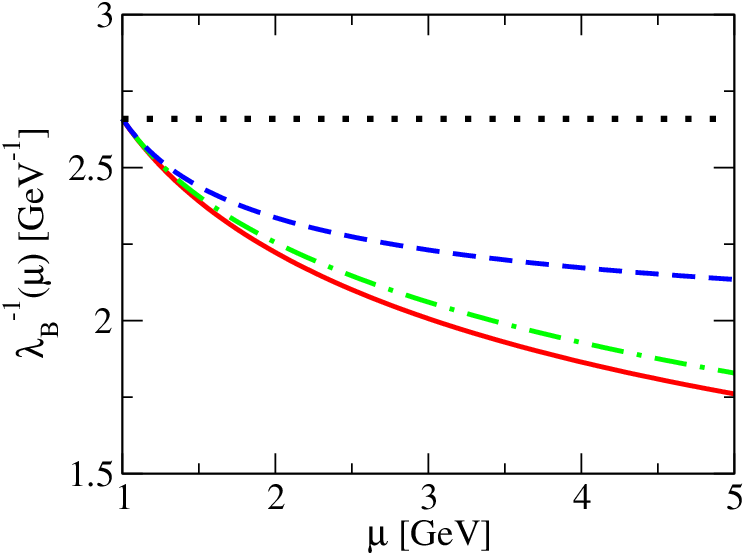
Our results of presented in Table 1 as well as those calculated at even higher are plotted by the solid curve in the first panel in Fig. 3, and, similarly, the solid curves in the other two panels show the behaviors of the logarithmic moments defined in the coordinate space, and of (54) and (55), with the NLL accuracy (43)-(46) using the input DA (71). Here, the dot-dashed curves present the fixed-order calculations based on (61)-(63) substituting , , and calculated with (71), and these results are modified into the dashed curves when we omit the double logarithmic correction behaving as , compared to the corresponding tree () contribution, in each coefficient of , , and in the RHS of (61)-(63). Furthermore, those results reduce to the dotted lines when . We find good accuracy of the fixed-order formulae (61)-(63), and thus the rapid convergence of the resummed perturbation theory in (53)-(55) with (43)-(46) when organized by of (41), whose behavior as a function of is shown by the solid curve in Fig. 4. On the other hand, in (61)-(63), the double logarithmic effects play important roles to determine the scale dependence of , , , while the other contributions tend to cancel to a large extent. As the result, the perturbative evolution from to can modify the values of those logarithmic moments considerably, by 20-30%. In Fig. 4, we also show the behavior of of (46) by the dashed curve; this demonstrates that the condition (60) is indeed satisfied, so that our formulae (53)-(55), as well as (35) giving their basis, describe the well-defined evolutions for all relevant scales.
@
In the present paper, we have discussed in detail the effects of the evolution on the -meson LCDA and on its integrals , , relevant to exclusive decays, emphasizing model-independent aspects revealed by our coordinate-space approach, but did not intend to determine the precise values of those integrals at . Such determination requires us to calculate the -meson LCDA (1) at the initial scale , reducing the corresponding theoretical uncertainty as much as possible: as found in our previous work [23], the corresponding initial LCDA, calculated in the form of (71), is significantly influenced by the novel HQET parameters and arising in the OPE form (65), which are associated with the dimension-5 quark-antiquark-gluon operators. Therefore, the rather large uncertainty in their existing estimate (70) based on QCD sum rules calls for more precise estimates of and . Recently, higher-order corrections to the QCD sum rules for and have been calculated, and these new contributions are found to improve the estimate of and [37]. We also note that in the RHS of (72), evaluated in Table 1, the second term is much larger than the first term. This suggests that , as well as , is rather sensitive to the functional form that models the LCDA in the long-distance region; for example, a functional form motivated by the so-called Wandzura-Wilczek approximation [21, 22] provides an interesting possible alternative to the form appearing in the second term in (71) (see, e.g., [38] for other studies on the behaviors of the LCDA). Systematic investigations of these points, combined with the evolution effects obtained in this paper, could determine the values of , , at as precisely as possible, and those results will be presented elsewhere.
VI Conclusions
In this paper, we have studied the RG evolution of the -meson LCDA, working in the coordinate-space representation of the LCDA. The corresponding evolution equation and its solution demonstrated that our coordinate-space approach has remarkable advantages over the conventional approach in the momentum space. Indeed, only in the coordinate space, the relevant kernel in the evolution equation, associated with the cusp anomalous dimension as well as the DGLAP-type anomalous dimension, is quasilocal, and this quasilocality is inherited by the corresponding analytic solution, leading to the simplest expression possible for calculating the evolution of the -meson LCDA. Our explicit formula of the solution has the accuracy beyond the one-loop level in the RG-improved perturbation theory, taking into account the effect of the two-loop cusp anomalous dimension according to consistent order counting, such that the Sudakov-type double logarithmic effects as well as the DGLAP-type single-logarithmic corrections are resummed at the NLL accuracy. This result, in turn, allowed us to derive the master formula, by which the relevant integrals of the LCDA at the scale , arising in the factorization formula for the exclusive -meson decays, can be reexpressed in a model-independent way by the compact integrals of the LCDA at a typical hadronic scale GeV.
We applied our evolution formula to the LCDA with the initial scale , which is determined by the OPE having the perturbative (NLO) accuracy consistent with the NLL-level resummation, and the highest nonperturbative accuracy, at present, taking into account the local operators of dimension . The quasilocal structure of our evolution guarantees that the -meson LCDA at a certain quark-antiquark distance is not contaminated under the change of the renormalization scale by the configurations of the quark and antiquark for the larger distances, so that the LCDA at high scales, obtained through our evolution from the OPE-based, initial LCDA that is accurate for interquark distances less than GeV-1, exhibits the model-independent behaviors for distances GeV-1. Our explicit numerical calculation indicated the considerable effects of the evolution, from the scale to , for the LCDA and its relevant integrals. In particular, we found that the dominant roles are played by the double logarithmic corrections, although particular attention was not paid to them in previous works. On the other hand, we observed the rapid convergence of the corresponding resummed perturbation series organized by the proper logarithmic expansion.
Using the information available for the nonperturbative effects associated with the OPE-based, initial LCDA, our evolution gave an estimate for the relevant integrals of the LCDA at the scale , e.g., GeV-1 at GeV. This is larger than the estimates by other works, inheriting the larger value GeV-1 in our case, which is induced by matrix elements of the dimension-5 quark-antiquark-gluon operators in the OPE for the initial LCDA. Combined with an update of the information on the nonperturbative effects in the initial LCDA, the results derived in this paper are immediately applicable for calculating the refined values of those integrals relevant to exclusive decays.
Appendix A The evolution in the momentum representation
The evolution of the -meson LCDA in the representation with the light-cone separation is provided by our solution (35) with the analytic continuation performed. We calculate the Fourier transformation of this result, in order to derive the evolution for the LCDA in the momentum representation (see (1)):
| (73) |
with the integration kernel,
| (74) |
where the integration over can be performed straightforwardly, yielding
| (75) |
Here, we have introduced the notation, . Changing the integration variable to and using with , we can rewrite (75) as
| (76) |
and we note that this can be expressed by the hypergeometric function,
| (77) | |||
| (78) |
where the first line shows the usual definition by the series expansion, and the second line gives the integral representation to be compared with (76). Substituting the result into (73), we obtain
| (79) |
which gives a well-defined formula when the condition (31) is satisfied. The evolution of the -meson LCDA in this form was first derived in [18, 20] by solving the evolution equation given in the momentum space, see (13), (14); note that and in the present paper correspond, respectively, to and in [18, 20]. We mention that it would not be straightforward to derive the relations (56)-(59) based on (79), because of the structure involving the complicated integration of the hypergeometric function (see [34]).
Acknowledgments
We thank V. M. Braun for valuable discussions. This work was supported by the Grant-in-Aid for Scientific Research No. B-19340063. The work of H.K. is supported in part by the UK Science & Technology Facilities Council under grant number PP/E007414/1.
References
- [1] M. Beneke, G. Buchalla, M. Neubert and C. T. Sachrajda, Phys. Rev. Lett. 83, 1914 (1999); Nucl. Phys. B591, 313 (2000); B606, 245 (2001).
- [2] C. W. Bauer, D. Pirjol and I. W. Stewart, Phys. Rev. Lett. 87, 201806 (2001); Phys. Rev. D65, 054022 (2002); D67, 071502 (2003); C. W. Bauer, D. Pirjol, I. Z. Rothstein and I. W. Stewart, Phys. Rev. D70, 054015 (2004).
- [3] H. n. Li and H. L. Yu, Phys. Rev. Lett. 74, 4388 (1995); Phys. Lett. B353, 301 (1995); Phys. Rev. D53, 2480 (1996); H. n. Li, Prog. Part. Nucl. Phys. 51, 85 (2003).
- [4] M. Antonelli et al., arXiv:0907.5386 [hep-ph].
- [5] G. P. Korchemsky, D. Pirjol and T. M. Yan, Phys. Rev. D61, 114510 (2000); S. W. Bosch and G. Buchalla, Nucl. Phys. B621, 459 (2002); JHEP 0208, 054 (2002); B. Grinstein and D. Pirjol, Phys. Rev. D73, 094027 (2006); D73, 014013 (2006); C. W. Bauer, I. Z. Rothstein and I. W. Stewart, Phys. Rev. D74, 034010 (2006); Y. Y. Keum, H. n. Li and A. I. Sanda, Phys. Lett. B504, 6 (2001); Phys. Rev. D63, 054008 (2001); T. Kurimoto, H. n. Li and A. I. Sanda, Phys. Rev. D65, 014007 (2002).
- [6] S. Descotes-Genon and C. T. Sachrajda, Nucl. Phys. B650, 356 (2003); Phys. Lett. B557, 213 (2003); E. Lunghi, D. Pirjol and D. Wyler, Nucl. Phys. B649, 349 (2003).
- [7] S. W. Bosch, R. J. Hill, B. O. Lange and M. Neubert, Phys. Rev. D67, 094014 (2003).
- [8] M. Beneke and T. Feldmann, Nucl. Phys. B592, 3 (2001).
- [9] M. Beneke and M. Neubert, Nucl. Phys. B675, 333 (2003); M. Beneke and S. Jager, Nucl. Phys. B751, 160 (2006); B768, 51 (2007); M. Beneke, T. Huber and X. Q. Li, Nucl. Phys. B832, 109 (2010).
- [10] N. Kivel, JHEP 0705, 019 (2007); V. Pilipp, Nucl. Phys. B794, 154 (2008); G. Bell, Nucl. Phys. B795, 1 (2008); B822, 172 (2008); G. Bell and V. Pilipp, Phys. Rev. D80, 054024 (2009).
- [11] A. Szczepaniak, E. M. Henley and S. J. Brodsky, Phys. Lett. B 243, 287 (1990); R. Akhoury, G. Sterman and Y. P. Yao, Phys. Rev. D50, 358 (1994).
- [12] A. G. Grozin and M. Neubert, Phys. Rev. D55, 272 (1997).
- [13] P. Ball and E. Kou, JHEP 0304, 029 (2003).
- [14] A. Khodjamirian, T. Mannel and N. Offen, Phys. Lett. B620, 52 (2005).
- [15] Unless otherwise indicated, the “moment” implies the one with respect to the momentum variable.
- [16] V. M. Braun, D. Y. Ivanov and G. P. Korchemsky, Phys. Rev. D69, 034014 (2004).
- [17] G. P. Korchemsky and A. V. Radyushkin, Nucl. Phys. B283, 342 (1987); I. A. Korchemskaya and G. P. Korchemsky, Phys. Lett. B287, 169 (1992).
- [18] B. O. Lange and M. Neubert, Phys. Rev. Lett. 91, 102001 (2003).
- [19] P. Ball, V. M. Braun and E. Gardi, Phys. Lett. B665, 197 (2008).
- [20] S. J. Lee and M. Neubert, Phys. Rev. D72, 094028 (2005).
- [21] H. Kawamura, J. Kodaira, C.F. Qiao and K. Tanaka, Phys. Lett. B523, 111 (2001); Erratum-ibid. B536, 344 (2002); Mod. Phys. Lett. A18, 799 (2003); Nucl. Phys. B (Proc. Suppl.) 116, 269 (2003).
- [22] T. Huang, X. G. Wu and M. Z. Zhou, Phys. Lett. B611, 260 (2005); B. Geyer and O. Witzel, Phys. Rev. D72, 034023 (2005).
- [23] H. Kawamura and K. Tanaka, Phys. Lett. B673, 201 (2009).
- [24] M. Neubert, Phys. Rept. 245, 259 (1994).
- [25] A. G. Grozin, Int. J. Mod. Phys. A20, 7451 (2005).
- [26] S. Descotes-Genon and N. Offen, JHEP 0905, 091 (2009).
- [27] Figure 1 (a) is IR-finite, while Figs. 1 (b), (c) produce the IR poles in the Feynman gauge. See [23] for the details.
- [28] I. I. Balitsky and V. M. Braun, Nucl. Phys. B 311, 541 (1989).
- [29] G. P. Lepage and S. J. Brodsky, Phys. Lett. B87, 359 (1979); A. V. Efremov and A. V. Radyushkin, Phys. Lett. B94, 245 (1980).
- [30] V. L. Chernyak and A. R. Zhitnitsky, Phys. Rept. 112, 173 (1984); V. M. Braun and I. E. Filyanov, Z. Phys. C48, 239 (1990); P. Ball, V. M. Braun, Y. Koike and K. Tanaka, Nucl. Phys. B529, 323 (1998).
- [31] J. Kodaira and L. Trentadue, Phys. Lett. B112, 66 (1982).
- [32] The RG evolution of the shape function for inclusive decays is described by the evolution operator of this type, see G. P. Korchemsky and G. Sterman, Phys. Lett. B340, 96 (1994); A. G. Grozin and G. P. Korchemsky, Phys. Rev. D53, 1378 (1996).
- [33] For example, see S. Catani, D. de Florian, M. Grazzini and P. Nason, JHEP 0307, 028 (2003); G. Bozzi, S. Catani, D. de Florian and M. Grazzini, Nucl. Phys. B 737, 73 (2006); H. Kawamura, J. Kodaira and K. Tanaka, Prog. Theor. Phys. 118, 581 (2007).
- [34] G. Bell and T. Feldmann, JHEP 0804, 061 (2008).
- [35] A. G. Grozin and M. Neubert, Nucl. Phys. B495, 81 (1997).
- [36] I. I. Y. Bigi, M. A. Shifman, N. G. Uraltsev and A. I. Vainshtein, Phys. Rev. D50, 2234 (1994); M. Beneke and V. M. Braun, Nucl. Phys. B426, 301 (1994).
- [37] T. Nishikawa and K. Tanaka, in preparation.
- [38] H. n. Li and H. S. Liao, Phys. Rev. D70 (2004) 074030; Y. Y. Charng and H. n. Li, Phys. Rev. D72, 014003 (2005); T. Kurimoto, Phys. Rev. D74, 014027 (2006); T. Huang, C. F. Qiao and X. G. Wu, Phys. Rev. D73, 074004 (2006); B. Geyer and O. Witzel, Phys. Rev. D76, 074022 (2007); A. Khodjamirian, T. Mannel and N. Offen, Phys. Rev. D75, 054013 (2007); A. Le Yaouanc, L. Oliver and J. C. Raynal, Phys. Rev. D77, 034005 (2008).