Clustering and variable selection for categorical multivariate data

Consider independent and identically distributed (iid) instances of a multivariate random vector $X=(X^{l})_{1\leq l\leq L}$, where the number of categorical variables $L$ is potentially large. We investigate two main settings:

1. 1.

   Each $X^{l}$ is a multinomial variable taking values in $\{1,\ldots,\ A_{l}\}$.

2. 2.

   Each $X^{l}$ consists of a (unordered) set $\{X^{l,1},\ X^{l,2}\}$ of two (possibly equal) qualitative variables taking their values in the same set $\{1,\ldots,\ A_{l}\}$.

Throughout this article, these two settings are referred to as Case 1 and Case 2. In both cases, numbers denoted by $A_{l}$ are assumed to be known and to satisfy $A_{l}\geq 2$.

Case 1 is generic, whereas Case 2 is more specific to multilocus data. Our results (presented below) could easily be extended to other kinds of discrete models, provided it is possible to compute the metric entropies as described in Section 3.

The studied sample is assumed to originate from a population structured into a certain (unknown) number $K$ of sub-populations (clusters), where each cluster is characterized by a set of category frequencies. The (unobserved) sub-population an individual comes from is denoted by the variable $Z$, which takes its values in the set $\{1,\ldots,k,\ldots,\ K\}$ of the different cluster labels. The distribution of $Z$ is given by the vector $\mathbf{\pi}=(\pi_{k})_{1\leq k\leq K}$, where $\pi_{k}=P(Z=k)$. Variables $X^{1},\ldots,\ X^{L}$ are assumed to be conditionally independent given $Z$. For Case 2, the $X^{l,1}$ and $X^{l,2}$ states of the $l^{\text{th}}$ variable are also assumed to be conditionally independent given $Z$. In accordance with these assumptions, the probability distribution of an observation $x=(x^{l})_{1\leq l\leq L}$ in a population $k$ is given in the following equations:

where $\alpha_{k,l,j}$ is the probability of the modality $j$ associated with the variable $X^{l}$ in population $k$. The mixing proportions $\pi_{k}$ and the probabilities $\alpha_{k,l,j}$ are treated as parameters.

These assumptions, which are considered classical in latent class model literature, are known as Linkage Equilibrium (LE) and Hardy-Weinberg Equilibrium (HWE) in the context of genomics. Such assumptions may seem simplistic because they disregard the migrations between populations and assume that the parents of a given individual are taken uniformly at random in the population to which the individual belongs. Nevertheless, these assumptions have proven useful in describing many population genetic attributes, and they continue to serve as a base model in the development of more realistic models of microevolution.

Simplified and misspecified models are often preferable to achieve greater precision with the oracle approach (as explained in the introduction). Use of these preferred models introduces a modeling bias in order to obtain more robust estimators and classifiers and also leads to a smaller estimation error. In particular, the introduction of covariances is unlikely to produce better estimates because it would increase the dimensions of the considered models. This fact also justifies the following simplification:

It is possible that the structure of interest is contained in only a subset $S$ of the available variables $L$; the other variables may be useless and could even hinder the detection of a reasonable clustering into statistically different populations. The frequencies of the categories are different in at least two populations for the variables in $S$; we refer to them as clustering variables. For the other variables, the categories are assumed to be equally distributed across the clusters. The simulations performed in Toussile and Gassiat (2009) illustrate the benefits of this approximation.

In our case, $\beta_{l,j}$ denotes the frequency of the category $j$ associated with the variable $X^{l}$ in the whole population:

Clearly, $S=\emptyset$ if $K=1$, otherwise $S$ belongs to $\mathcal{P}^{*}(L)$, which is the set of all nonempty subsets of $\{1,\ldots,L\}$.

Summarizing these assumptions, we can express the likelihood of an observation $x=(x^{l})_{1\leq l\leq L}$:

where $\theta=(\mathbf{\pi},\mathbf{\alpha},\mathbf{\beta})$ is a multidimensional parameter with

For a given $K$ and $S$, $\theta=\theta_{(K,\,S)}$ ranges in the set

where $\mathbb{S}_{r-1}=\{p=(p_{1},\ p_{2},\ldots,\ p_{r})\in[0,\ 1]^{r}:\sum_{j=1}^{r}p_{j}=1\}$ is the $(r-1)$-dimensional simplex.

Then, we consider the collection of all parametric models

with $(K,\,S)\in\mathcal{C}:=\{(1,\emptyset)\}\cup(\mathbb{N}\backslash\{0,1\})\times\mathcal{P}^{*}(L)$. To minimize the use of notations, we make frequent use of the single index $m\in\mathcal{C}$ instead of using $(K,\,S)$.

Each model $\mathcal{M}_{(K,\,S)}$ corresponds to a particular structure situation with $K$ clusters and a subset $S$ of clustering variables. Inferring $K$ and $S$ presents a model selection problem in a density estimation framework and also leads to data clustering through the estimation $\widehat{\theta}$ of the parameter $\theta_{(K,\,S)}$ and the prediction of the class $z$ of an observation $x$ by the MAP method:

Our study implements the maximum likelihood estimator (MLE). For each model $\mathcal{M}_{(K,S)}$, the MLE corresponds to the minimum contrast estimator$\widehat{P}_{(K,S)}=P_{(K,\,S,\widehat{\theta})}$ of the log-likelihood contrast

The Kullback-Leibler divergence $\KL$ provides a suitable risk function that measures the quality of an estimator in a density estimation. However, this divergence also has disadvantages in the context of a discrete framework; in fact, the MLE assigns a zero probability to any unobserved categories in the sample. Consequently, the Kullback-Leibler risk

is infinite. In the following, we therefore consider a slightly different collection $\mathcal{C}^{\varepsilon}$ of competing models $\mathcal{M}_{m}^{\varepsilon}$ coupled with a threshold on the parameters of $\varepsilon>0$ :

Such models disqualify probability distributions that assign too low of a probability (particularly zero) to certain categories. A good choice of $\varepsilon$ can result in the same collection of maximum likelihood estimators with a probability tending to one, as was demonstrated by a result obtained in (Toussile and Gassiat, 2009, Appendix D): if the true probability $P_{0}$ of the observations is positive, then for any $(K,\,S)$ a real $\varepsilon=\varepsilon_{K,S}>0$ exists, such that

where $\widehat{P}_{(K,\,S)}$ is the MLE in a non-truncated model.

For the sake of simplicity, $\mathcal{M}_{(K,S)}^{\varepsilon}$ is also denoted by $\mathcal{M}_{(K,S)}$, and $\widehat{P}_{(K,\,S)}$ represents a minimizer of the contrast $\gamma_{n}$ within $\mathcal{M}_{(K,S)}^{\varepsilon}$. Additionally, because we cannot discover more than $n$ clusters from an $n$-sample, we only consider the models indexed by $(K,S)$ for which the number of clusters $K$ is smaller than the sample size $n$.

Let $(K^{*},\,S^{*})$ be a minimizer over $(K,\,S)$ of the Kullback-Leibler risk (6). The ideal candidate density $\widehat{P}_{(K^{*},\,S^{*})}$, or oracle density, is not accessible because it is dependent on the (unknown) true density $P_{0}$. The oracle density is used as a benchmark to quantify the quality of our model selection procedure: the simulation performed in paragraph 5.2 compares the Kullback-Leibler risk of the selected estimator $\widehat{P}_{(\widehat{K}_{n},\ \widehat{S}_{n})}$ with the oracle risk.

Minimization of a penalized contrast is a common method to solve model selection problems. The selected model $\mathcal{M}_{(\widehat{K}_{n},\widehat{S}_{n}}$ is a minimizer of a penalized criterion of the form

in which $\pen_{n}:\ \mathcal{C}\rightarrow\mathbb{R}_{+}$ is the penalty function. Eventually, the selected estimator becomes $\widehat{P}_{(\widehat{K}_{n},\ \widehat{S}_{n})}$.

The penalty function is designed to avoid over-fit problems. Classical penalties, such as those used in $\AIC$ and $\BIC$ criteria, are based on model dimensions. In the following, we refer to the number of free parameters

as the dimension of the model $\mathcal{M}_{(K,\,S)}$. The penalty functions of $\AIC$ and $\BIC$ are respectively defined by

Our main result provides an oracle inequality for Case 1 and Case 2. This inequality links the Hellinger risk $\mathrm{E}_{P_{0}}[\h^{2}(P_{0},\widehat{P}_{(\widehat{K}_{n},\widehat{S}_{n})})]$ of the selected estimator to the Kullback-Leibler divergence $\KL$ between the true density and each model in the model collection. Recall that for two probability distributions $P$ and $Q$, and given $s$ and $t$ as density functions with respect to a common $\sigma$-finite measure $\mu$, the Hellinger distance between $P$ and $Q$ is the quantity $\h(P,Q)$ defined by

Unlike $\KL$, which is not a metric, the Hellinger distance $\h$ allowed us to take advantage of the metric properties (metric entropy) of the models. Use of the metric entropy may be avoided by directly investigating Talagrand’s inequality, which forms the basis of our study. Such an investigation may then lead to an oracle inequality directly on the Kullback-Leibler risk (6) and with explicit constants; this remains to be done in our context. See (Maugis and Michel, 2011a, S 2.2) for more insight regarding this topic.

We use the condition $\xi\leq 1$ to avoid more complicated calculations in our proof. In practice, $\xi$ is very likely to be smaller than $1$ (unless $L$ is very small).

Consider the following:

• •

  Theorem 1 is a density estimation result: it quantifies the quality of the parameter estimation, which defines the mixture density components. However, it is not easily connected to a classification result.

• •

  The leading term of the penalty for large $n$ is $\kappa\tfrac{\ln n}{2}\,\tfrac{D_{(K,\,S)}}{n}$, which is a $\BIC$ type penalty function. Consequently, we can apply Theorem 2 from Toussile and Gassiat (2009): when the underlying distribution $P_{0}$ belongs to one of the competing models, the smallest model $(K_{0},S_{0})$ containing $P_{0}$ is selected with a probability tending to $1$ as $n$ approaches infinity.

• •

  Such a penalty is not surprising in our context; it is, in fact, very similar to the penalty obtained by Maugis and Michel (2011a) for a Gaussian mixture framework.

• •

  Sharp estimates of $\kappa$ are not available. In practice, Theorem 1 is too conservative and leads to an over-penalized criterion that is outperformed by smaller penalties. Therefore, Theorem 1 is mainly used to suggest the shape of the penalty function

  $$\pen_{n}(K,\,S)=\lambda\,\frac{D_{(K,\,S)}}{n}$$

  (10)

  where the parameter $\lambda$ is chosen depending on $n$ and the collection $\mathcal{C}$ — but not on $(K,S)$. Slope heuristics (Birgé and Massart, 2007; Arlot and Massart, 2009) can be used in practice to calibrate $\lambda$. This is done in Section 4, where we use change-point detection (Lebarbier, 2002, see) in connection with slope heuristics.

• •

  Because $\h^{2}$ is upper bounded by $2$, the non-asymptotic feature of Theorem 1 becomes important when $n$ is large enough with respect to $D_{(K,\,S)}$. But even with small values of $n$, the simulations performed in Subsection 5 show that the penalized criterion that is calibrated by using slope heuristics maintains good behavior.

Theorem 1 is obtained from (Massart, 2007, Theorem 7.11), whose research investigated model selection problems by proposing penalty functions related to geometrical properties of the models, namely metric entropy with bracketing for the Hellinger distance.

We examine the following framework: Consider some measurable space $(A,{\mathcal{A}})$, and $\mu$ as a $\sigma$-finite positive measure on $A$. A collection of models $(\mathcal{M}_{m})_{m\in\mathcal{C}}$ is given, where each model $\mathcal{M}_{m}$ is a set of probability density functions $s$ with respect to $\mu$. The following relation permits us to extend the definition of $\h$ to the positive functions $s$ or $t$, whose integral is finite but not necessarily $1$. The function defined by $\sqrt{s}(x)=\sqrt{s(x)}$ is denoted by $\sqrt{s}$, and $\|\cdot\|_{2}$ denotes the usual norm in $\mathbb{L}^{2}(\mu)$; then

To restate the definition of metric entropy with bracketing, consider some collection $F$ of measurable functions on $A$ and $d$ as one of the following metrics on $F$: $\h$, $\|\cdot\|_{1}$, or $\|\cdot\|_{2}$. A bracket $[l,u]$ is the collection of all measurable functions $f$ such that $l\leq f\leq u$. Its $d$-diameter is the distance $d(u,l)$. Then, for every positive number $\varepsilon$, $N_{[\cdot]}(\varepsilon,F,d)$ denotes the minimal number of brackets whose $d$-diameter is no larger than $\varepsilon$, which is required to cover $F$. The $d$-entropy with bracketing of $F$ is defined as the logarithm of $N_{[\cdot]}(\varepsilon,F,d)$ and is denoted by $H_{[\cdot]}(\varepsilon,F,d)$.

We assume that for each model $\mathcal{M}_{m}$ the square entropy with bracketing $\sqrt{H_{[\cdot]}(\varepsilon,\mathcal{M}_{m},\h)}$ is integrable at $0$. Consider some function $\phi_{m}$ on $\mathbf{R}_{+}$ with the following properties:

1. (I).

   $\phi_{m}$ is nondecreasing, $x\mapsto\phi_{m}(x)/x$ is nonincreasing on $(0,+\infty)$ and for every $\sigma\in\mathbf{R}_{+}$ and every $u\in\mathcal{M}_{m}$

   $$\int_{0}^{\sigma}\sqrt{H_{[\cdot]}\left(x,S_{m}(u,\sigma),\h\right)}\mathbf{d}x\leq\phi_{m}(\sigma),$$

   where $S_{m}(u,\sigma)=\{t\in\mathcal{M}_{m}:\|\sqrt{t}-\sqrt{u}\|_{2}\leq\sigma\}$.

(I) is satisfied, in particular with $\phi_{m}(\sigma)=\int_{0}^{\sigma}\sqrt{H_{[\cdot]}(x,\mathcal{M}_{m},\h)}\mathbf{d}x$.

Massart (2007) stated a separability condition, which was denoted (M) in the text, to avoid measurability problems. This condition is easy to verify in our context and we omit it for greater legibility of the theorem.

Concerning Theorem 2, Massart (2007) explained that $\sigma_{m}^{2}$ has the role of a variance term of $\widehat{s}_{m}$, whereas the weights $x_{m}$ take into account the number of models $m$ of the same dimension.

In order to apply Theorem 2, we have to compute the metric entropy with bracketing of each model $\mathcal{M}_{(K,\,S)}$. This calculation is performed in the following result for which we provide the proof in Appendix A.

The technical quantity $C_{(K,\,S)}$ measures the complexity of a model $\mathcal{M}_{(K,\,S)}$.

The next step establishes an expression for $\phi_{m}$. Proof for all subsequent results is provided in Appendix B.

To avoid more complicated expressions, we do not define $\phi_{m}$ for $\sigma$ bigger than $\eta_{L}(1)$. A condition on $\xi$ therefore appears in the following lemma:

The condition appearing in Lemma 1 is fulfilled unless $L$ is very small, which is not the case for the usual applications.

We can deduce an upper bound for $\sigma_{m}$ based on Proposition 2 with a similar reasoning to Maugis and Michel (2011a). First, $\sigma_{m}\leq\eta_{L}(1)$ implies $\eta_{L}^{-1}(\sigma_{m})\leq 1$, and we obtain the lower bound $\sigma_{m}\geq\widetilde{\sigma}_{m}$, where

This can be used to get an upper bound

We then choose the weights $x_{m}$. For values bigger than $n\sigma_{m}^{2}$, this will change the shape of the penalty in Theorem 2. We define

The following lemma shows that this is a suitable choice.

We must lower bound $\eta_{L}^{-1}(\widetilde{\sigma}_{m})$ to express the penalty function, which is accomplished in the following lemma.

We finally use Theorem 2 to complete the proof of Theorem 1.

Theorem 1 suggests to use a penalty function of the shape given in equation (10), where modulo is defined as a multiplicative parameter $\lambda$ that has to be calibrated. Slope heuristics, as presented in Birgé and Massart (2007) and Arlot and Massart (2009), provide a practical method to find an optimal penalty $\pen_{\mathrm{opt}}(m)=\lambda_{\mathrm{opt}}D_{m}/n$. These heuristics are based on the conjecture that a minimal penalty $\pen_{\min}(m)=\lambda_{\min}D_{m}/n$ exists that is required for the model selection procedure: when the penalty is smaller than $\pen_{\min}$, the selected model is one of the most complex models, and the risk of the selected estimator is large. In contrast, when the penalty is larger than $\pen_{\min}$, the selected model is considerably less complex. Thus, the optimal penalty is close to twice the minimal penalty:

An explanation of the heuristics behind this factor $2$ can be found in Maugis and Michel (2011b), for instance. The name “slope heuristics” is derived from $\lambda_{\min}$, which is the slope of the linear regression $\gamma_{n}(\widehat{P}_{m})\sim D_{m}/n$ for a certain sub-collection of the most competitive models $m$. For example, in Figure 1(a) below, models containing the true one $\mathcal{M}_{(K_{0},\ S_{0})}$ exhibit a slope. This example also illustrates that slope heuristics are appropriate in our modeling context.

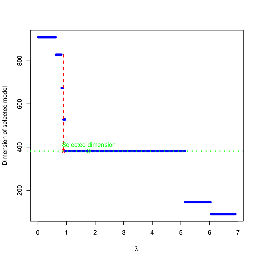
Instead of using linear regression to estimate $\lambda_{\min}$, we use another method (generally referred to as the dimension jump method) to detect the biggest jump on the selected dimension with respect to the candidate values of $\lambda$. In practice, we would assume a reasonable grid $\lambda_{1}<\cdots<\lambda_{n_{\lambda}}$ of $n_{\lambda}$ candidate estimates of $\lambda_{\min}$ and a sub-collection $\mathcal{C}_{ex}$ comprising the most competitive models. Each $\lambda_{i}$ leads to a selected model $\widehat{m}_{i}$ with dimension $D_{\widehat{m}_{i}}$. If $D_{\widehat{m}_{i}}$ is plotted as a function of $\lambda_{i}$, $\lambda_{min}$ is expected to lie at the position of the biggest jump.

However, Fig. 1(b) illustrates an important point: in this example the biggest jump occurs at $\lambda\approx 5.1$, but the optimal value of $\lambda_{\min}$ is around $0.9$, which corresponds to several successive jumps. We propose an improved version of the dimension jump method of Arlot and Massart (2009) based on a sliding window: on the axis of $\lambda$, we consider the sum of all jumps in a sliding window of size $h>0$. In Algorithm 1 below, which describes the procedure, $n_{h}$ denotes the number of candidate values of $\lambda_{\min}$ in the sliding window. We do not claim that this improves slope heuristics per se; we merely note that the proposed procedure improves the stability of the method in our simulations. In practice, following repeated trials, we choose a window of size $h=0.10$.

For a given maximum number of clusters $K_{\max}$, the number of competing models is equal to $1+(K_{\max}-1)*(2^{L}-1)$. Because this is a very large number in most situations, it would be very laborious to consider the total number of potentially applicable models to calibrate the parameter $\lambda$. Nevertheless, a sufficient number of models is necessary to ensure a clear jump in the selected dimension sequence. We therefore consider the modified backward-stepwise algorithm proposed in Toussile and Gassiat (2009), which enables us to gather the most competitive models among all possible $S$ for a given number of clusters $K$ and a given penalty function $\pen_{n}$. This algorithm also offers the possibility to add a complementary exploration step based on a similarly modified forward strategy: we refer to this algorithm as $explorer(K,\ \pen_{n})$.

Because the final penalty during the exploration step is unknown, we consider a reasonable grid $\frac{1}{2}=\lambda_{1}<\cdots<\lambda_{n_{\lambda}}=\ln n$ containing both penalty functions associated with $\AIC$ and $\BIC$. Each value $\lambda_{i}$ is associated with a penalty function $\pen_{\lambda_{i}}$. We launch $explorer(K,\ \pen_{\lambda_{i}})$ for all values of $K$ in $\{1,\ldots,\ K_{\max}\}$ and for all values of $\lambda_{i}$ of the grid; we then gather the explored models in $\mathcal{C}_{ex}$. This sub-collection appears to contain the most competitive models and it was therefore used to calibrate $\lambda$.

We consider a setting of $L=10$ variables with $10$ categories each. Each dataset is simulated as a mixture of $K_{0}=5$ populations in equal proportions. The simulation parameters are chosen so that the differentiation between populations, as measured by a population genetics parameter $F_{st}$ (a measure of genetic differentiation), decreases with the variable rank. Populations are distinctly separated for the first $6$ variables; for the next $2$ variables populations are poorly differentiated; the last $2$ variables follow the uniform distribution for all populations. The complete parameter is available at http://www.math.u-psud.fr/~toussile/. The overall differentiation occurs in a range considered difficult for clustering of such data (Latch et al., 2006). We examine different values of the sample size $n$ in $[100,\ 1000]$, and $30$ datasets are simulated for each value. Results are summarized in Fig. 2.

We observe similar behaviors of $\BIC$ and $\ICL$ in these experiments: both criteria perform poorly for the selection of variables and the classification of small sample sizes. In fact, Nadif and Govaert (1998) have pointed out that $\BIC$ requires a large sample size to reach its asymptotic behavior in a discrete framework. The high variability of the dimensions of the competing models, which cancels the contribution of the entropy term in $\ICL$, may explain the similar behavior of $\BIC$ and $\ICL$. In contrast, $\AIC$ and the newly proposed criterion are most suited to the selection of variables for both small and large sample sizes. The new criterion also performs well for the selection of the number of components for both small and large sample sizes, but $\AIC$ overestimates the number of components for large sample sizes (from $n=400$). As expected, the data-driven calibration of the penalty function globally improves the performance of the selection procedure and consequently provides an answer to the question “Which penalty for which sample size?”

Small variations in the results obtained for small sample sizes may occur from one run to another. In fact, the EM algorithm may fail to identify the global maximum for such sample sizes, in particular for models of larger dimensions. This is probably the case for some datasets of size $n\leq 300$; the number of free parameters in our simulated model is $\geq 310$.

As previously mentioned, the new criterion is designed in a density estimation framework. The following section compares the risks of the selected estimators. Our simulations consist of $101$ datasets with $L=6$ variables, $3$ categories for each variable, and $K_{0}=3$ components in equal proportions. The simulation parameters are chosen in such a way that the differentiation between the components is significant for the first $3$ variables and very small for the $4^{\text{th}}$ and $5^{\text{th}}$ variables, whereas the $6^{\text{th}}$ variable follows the uniform distribution for all components. Thus, the true model is defined by $K_{0}=3$ and $S_{0}=\{1,\ 2,\ 3,\ 4,\ 5\}$. The complete parameter is available at http://www.math.u-psud.fr/~toussile/.

The Kullback risk is estimated using a Monte Carlo procedure for $100$ simulated datasets, each with a sample size of $600$. Our results are summarized in Fig. 3 and Table 1.

Unsurprisingly, concerning the Kullback risk, the least favorable behavior originates from $\ICL$, followed by $\BIC$. In fact, these criteria are not designed to retrieve the minimal risk estimator. In addition, $\ICL$ and $\BIC$ are based on asymptotic approximations and may require large sample sizes. In contrast, the new criterion with a data-driven calibration of the penalty function performes significantly better (see Table 1). As stated previously, both $\AIC$ and the new criterion are designed to find the minimizer of the Kullback risk. Yet, similarly to $\BIC$ and $\ICL$, $\AIC$ is based on asymptotic approximations. The new criterion is designed from a non-asymptotic perspective, which may explain its advantage over $\AIC$.

The data set entitled “1984 United States Congressional Voting Records Database” includes votes of the U.S. House of Representatives Congressmen on $16$ key issues (disability, religion, immigration, army, education, …) identified by the Congressional Quarterly Almanac (CQA) in Asuncion and Newman (2007). This data set has $n=435$ instances ($267$ Democrats and $168$ Republicans). For each vote, three possible responses are taken into account: for, against, and abstention. The model selection procedure with calibration of the penalty function is applied to these data. The maximum number of clusters is set to $K_{\max}=10$. The selected number of clusters is $\widehat{K}_{n}=6$, and the selected subset of relevant variables does not include votes on disability and army issues. The confusion matrix comparing the obtained partition and the Democrat/Republican bi-partition is given in Table 2. More than $91\%$ of clusters $3$ and $4$ are Republicans, whereas more than $94\%$ of clusters $1$, $5$, and $6$ are Democrats. Republicans and Democrats are equally represented in cluster $2$. The subdivision of the two main parties into various tendencies, a common occurrence in politics, is reflected in these results.

We consider a collection of $27$-locus genotypes from $600$ individuals representing $20$ chicken breeds ($30$ individuals per breed). These data have been described in Rosenberg et al. (2001) in the context of a clustering method evaluation of multilocus genotypes. Of the $27$ loci, we consider $15$ that have no missing data. The data illustrate a very common difficulty with biologic datasets: the dimensions of the considered models are very large with respect to the number of individuals (note, however, that the dimensions of the competing models are large because we have 15 variables resulting in 600x2x15 = 18 000 individual measures). Nevertheless, our procedure resulted in an interesting classification: $17$ clusters correspond mostly to the initial breeds, and three of the clusters contain $2$ breeds each. The similarity between the obtained classification and the breeds as measured by the Rand index is greater than $98\%$. All loci are selected to be useful for clustering purposes. In Rosenberg et al. (2001), the authors found $18$ clusters by using the available $27$ variables. Their algorithm requires the user to perform several steps. The clusters they found also corresponded mostly to the initial breeds.

References

- Arlot and Massart (2009) [author] Arlot, SylvainS. and Massart, PascalP. (2009). Data-driven calibration of penalties for least-squares regression. J. Mach. Learn. Res. 10 245–279.
- Asuncion and Newman (2007) [author] Asuncion, A.A. and Newman, D. J.D. J. (2007). UCI Machine Learning Repository.
- Bai, Rao and Wu (1999) [author] Bai, Z.Z., Rao, C. R.C. R. and Wu, Y.Y. (1999). Model selection with data-oriented penalty. J. Statist. Plann. Inference 77 102–117. MR1677811
- Biernacki, Celeux and Govaert (2000) [author] Biernacki, C.C., Celeux, G.G. and Govaert, G.G. (2000). Assessing a mixture model for clustering with the integrated completed likelihood. IEEE Trans. Pattern Anal. 22 719–725.
- Birgé and Massart (2007) [author] Birgé, LucienL. and Massart, PascalP. (2007). Minimal penalties for Gaussian model selection. Probab. Theory Related Fields 138 33–73. MR2288064
- Celeux and Govaert (1991) [author] Celeux, GillesG. and Govaert, GérardG. (1991). Clustering criteria for discrete data and latent class models. J. Classif. 8 157–176. 10.1007/BF02616237
- Celeux, Hurn and Robert (2000) [author] Celeux, GillesG., Hurn, MerrileeM. and Robert, Christian P.C. P. (2000). Computational and inferential difficulties with mixture posterior distributions. J. Am. Stat. Assoc. 95 957–970. MR1804450
- Chen, Forbes and Francois (2006) [author] Chen, C.C., Forbes, F.F. and Francois, O.O. (2006). Fastruct: Model-based clustering made faster. Molecular Ecology Notes 6 980–983.
- Collins and Lanza (2010) [author] Collins, Linda M.L. M. and Lanza, Stephanie T.S. T. (2010). Latent Class and Latent Transition Analysis: With Applications in the Social, Behavioral, and Health Sciences. Wiley Series in Probability and Statistics. Wiley.
- Corander et al. (2008) [author] Corander, JukkaJ., Marttinen, PekkaP., Sirén, JukkaJ. and Tang, JingJ. (2008). Enhanced Bayesian modelling in BAPS software for learning genetic structures of populations. BMC Bioinformatics 9 539.
- Dempster, Lairdsand and Rubin (1977) [author] Dempster, A. P.A. P., Lairdsand, N. M.N. M. and Rubin, D. B.D. B. (1977). Maximum likelihood from incomplete data via the EM algorithm. J. Royal Statist. Soc. Series B 39 1–38. MR0501537
- Genoveve and Wasserman (2000) [author] Genoveve, C. R.C. R. and Wasserman, LarryL. (2000). Rates of convergence for the Gaussian mixture sieve. Ann. Statist. 28 1105–1127. MR1810921
- Goodman (1974) [author] Goodman, Leo A.L. A. (1974). Exploratory latent structure analysis using both identifiable and unidentifiable models. Biometrika 61 215–231. MR0370936
- Latch et al. (2006) [author] Latch, E. K.E. K., Dharmarajan, GuhaG., Glaubitz, Jeffrey C.J. C. and Rhodes, Olin E.O. E. Jr. (2006). Relative performance of Bayesian clustering software for inferring population substructure and individual assignment at low levels of population differentiation. Conservation Genetics 7 295.
- Lebarbier (2002) [author] Lebarbier, ÉmilieÉ. (2002). Quelques approches pour la détection de rupture à horizon fini PhD thesis, Univ Paris-Sud, F-91405 Orsay.
- Massart (2007) [author] Massart, PascalP. (2007). Concentration inequalities and model selection. Lecture Notes in Mathematics 1896. Springer-Verlag, Berlin. MR2319879
- Maugis and Michel (2011a) [author] Maugis, CathyC. and Michel, BertrandB. (2011a). A non asymptotic penalized criterion for Gaussian mixture model selection. ESAIM: P&S 15 41–68. MR2870505
- Maugis and Michel (2011b) [author] Maugis, CathyC. and Michel, BertrandB. (2011b). Data-driven penalty calibration: A case study for Gaussian mixture model selection. ESAIM: P&S 15 320–339. MR2870518
- McCutcheon (1987) [author] McCutcheon, A. L.A. L. (1987). Latent Class Analysis. Quantitative Applications in the Social Sciences 64. Sage Publications, Thousand Oaks, California.
- McLachlan and Peel (2000) [author] McLachlan, GeoffreyG. and Peel, DavidD. (2000). Finite Mixture Models. Wiley Series in Probability and Statistics. Wiley. MR1789474
- Nadif and Govaert (1998) [author] Nadif, M.M. and Govaert, GérardG. (1998). Clustering for binary data and mixture models – choice of the model. Appl. Stoch. Models Data Anal. 13 269–278.
- Pritchard, Stephens and Donnelly (2000) [author] Pritchard, J. K.J. K., Stephens, M.M. and Donnelly, P.P. (2000). Inference of population structure using multilocus genotype data. Genetics 155 945–59.
- Rigouste, Cappé and Yvon (2006) [author] Rigouste, LoïsL., Cappé, OlivierO. and Yvon, FrançoisF. (2006). Inference and evaluation of the multinomial mixture model for text clustering. Inform. Process. Manag. 43 1260–1280.
- Rosenberg et al. (2001) [author] Rosenberg, Noah A.N. A., Burke, TerryT., Elo, KariK., Feldman, Marcus W.M. W., Freidlin, Paul J.P. J., Groenen, Martien A. M.M. A. M., Hillel, JossiJ., Ma, AskoA., Vignal, AlainA., Wimmers, KlausK. and Weigend, SteffenS. (2001). Empirical evaluation of genetic clustering methods using multilocus genotypes from 20 chicken breeds. Biotechnology.
- Toussile and Gassiat (2009) [author] Toussile, WilsonW. and Gassiat, ElisabethE. (2009). Variable selection in model-based clustering using multilocus genotype data. Adv. Data Anal. Classif. 3 109–134. MR2551051
- Verzelen (2009) [author] Verzelen, NicolasN. (2009). Adaptative estimation to regular Gaussian Markov random fields PhD thesis, Univ Paris-Sud.
- Villers (2007) [author] Villers, F.F. (2007). Tests et selection de modèles pour l’analyse de données protéomiques et transcriptomiques PhD thesis, Univ Paris-Sud.