1Introduction

arXiv:0808.????

String Theory and Water Waves

Ramakrishnan Iyer^♮, Clifford V. Johnson^♭, Jeffrey S. Pennington^♯

^♮,♭Department of Physics and Astronomy

University of Southern California

Los Angeles, CA 90089-0484, U.S.A.

^♯SLAC National Accelerator Laboratory

Stanford University

Stanford, CA 94309, U.S.A.

^♮ramaiyer, ^♭johnson1, [at] usc.edu; ^♯jpennin [at] stanford.edu

Abstract

We uncover a remarkable role that an infinite hierarchy of non–linear differential equations plays in organizing and connecting certain ${\hat{c}}<1$ string theories non–perturbatively. We are able to embed the type 0A and 0B $(A,A)$ minimal string theories into this single framework. The string theories arise as special limits of a rich system of equations underpinned by an integrable system known as the dispersive water wave hierarchy. We observe that there are several other string–like limits of the system, and conjecture that some of them are type IIA and IIB $(A,D)$ minimal string backgrounds. We explain how these and several string–like special points arise and are connected. In some cases, the framework endows the theories with a non–perturbative definition for the first time. Notably, we discover that the Painlevé IV equation plays a key role in organizing the string theory physics, joining its siblings, Painlevé I and II, whose roles have previously been identified in this minimal string context.

1 Introduction

While string theory has had remarkable successes over the last several years, accelerated by the revolutions in understanding its non–perturbative properties, it is still very much the case that we do not yet know what the theory is. We cannot state unambiguously what the basic degrees of freedom are (it is highly context dependent in a way that depends upon the dynamics themselves), and even the backgrounds in which the theory propagates are themselves open to interpretation. For example, in some descriptions and situations, the theory contains gravity, and in others, it does not. From some perspectives there are open strings present, and from others, only closed. Ironically, several of these frustrating (from the point of view of finding simple definitions) features are also among the theory’s most powerful positive traits, allow an ever–widening range of applications of the theory to diverse problems, often of a strongly coupled nature.

While applications continue, it is still important to try to get to grips with what the theory is. At the very least, this is important from a pragmatic standpoint, since perhaps a useful definition or characterization of string theory might be put to use as, for example, a diagnostic device in identifying when a physical problem may have some aspect of it that is amenable to solution by string theory methods. More generally, if string theory ultimately plays some fundamental role in the understanding of physics beyond the standard model, and/or in cosmology and other origins questions about the universe at large, a more profound understanding of the nature, power, and scope of the theory would seem to be highly desirable.

At best, to date, as a result of various dualities, we know that it is probably part of some larger physical framework which itself is only string theoretic in various corners of its parameter space. This physical setting, called M–theory, remains profoundly mysterious well over a decade after the first clear glimpses of it[1, 2, 3].

Historically, problems pertaining to such essential matters of understanding in physics are greatly illuminated by having a rich set of examples that are simple, but yet complex enough to contain all the important phenomena in question. For the problems outlined above, it would be rather excellent to have the simplest possible string theories that still contain some of the marvellous non-perturbative physics we know and love, and be able to follow them as they connect to each other in ways that are entirely invisible in perturbation theory. Further icing on the cake would be to have the physics all captured in terms of relatively familiar structures for which there is an existing technology for its study.

This is the subject of this paper (and a follow–up to appear later[4]), at least in part. The simplest known strings with tractable non–perturbative physics that contain a rich set of phenomena (such as holography and open–closed dualities) are the minimal strings[5, 6, 7], and in particular (where non–perturbative physics is concerned) the type 0 strings (formulated in refs.[8, 9, 10, 11, 12] and refs.[13, 14], and recognized as type 0 strings in ref.[15]). The non–perturbative formulation of the type 0A and type 0B strings can be done rather beautifully in terms of certain integrable systems, as we will review later: Type 0A has the Korteweg–de Vries system while type 0B has Zakharov–Shabat. The non–perturbative physics of each is formulated in terms of associated non–linear ordinary differential equations often called “string equations”. While much of the language of the two is similar, these are very different systems, and except for various accidental (from the perspective of those separate formulations) perturbative coincidences (and a non–trivial non–perturbative equivalence for one model — see later), the physics of each are quite separate indeed.

This paper builds on all of these results, taking them much further. We have found that there is a larger framework into which the type 0A and type 0B string theories can be naturally embedded and within which they are connected as parts of a larger theory. We found further that the two string theories are merely special points in a much larger tapestry of possibilities. When perturbation theory is examined, other special points suggest themselves, and they turn out to be just as “stringy” as the original type 0 theories, deserving to be thought of as string theories as well. We begin the program of trying to identify some of these theories, with some success. We also find that the larger framework provides natural definitions of regimes of the type 0 string theories that are hard to define using perturbation theory, and we will report more fully on non–perturbative aspects in a follow–up paper[4].

In this sense, we have a precise analogue of M–theory. We have a larger physical framework that is not itself a string theory, but that can be readily specialized to yield string theories as special limits. We can move between different theories in a quite natural way, which is nonetheless outside the framework of any of its daughter string theories. We find this encouraging and exciting.

At the base of our infinite family of string equations, organizing much of this remarkable structure, is a non--linear differential equation known as Painlevé IV. This well--known equation from the classical mathematics literature¹¹ 1 See for example the lovely monograph of ref.[16] and references therein., part of a celebrated family of six equations, has two arbitrary constants, usually denoted $\alpha$ and $\beta$ . (Actually, two copies of Painlevé IV turn up in our story, intertwined in an interesting way.) It turns out that the type 0A and 0B points in the tapestry of theories occur at the vanishing of one or other of these constants for one of the copies of Painlevé IV. The vanishing of the constants of the second Painlevé IV hint at interesting new special points.

After reviewing crucial aspects of the type 0A and 0B string theories in section 2, we unpack the dispersive water wave hierarchy and present the infinite family of equations we propose as the string equations in section 3. Section 4 highlights the role of Painlevé IV. In section 5 we show how the structures of section 2 arise as special points in this larger framework, while section 6 is a detailed study of the rich properties of the string equations and the types of solutions available. We organize and classify a great deal of the physics that appears, and notice in section 7 that much of the physics can be organized in terms of a square. The square is reminiscent of the main square organizing the moduli space of ${\hat{c}}=1$ (two–dimensional) string theories, discovered in ref.[17], and we contemplate a possible connection, perhaps induced by Renormalization Group flow[18, 19] to the ${\hat{c}}<1$ context of the work in question. The possible relation between the squares helps us make a conjecture about the nature of two new special points we find: They might be type IIA and IIB minimal string theories. (Note that these are type II theories in the sense of the structure of the GSO projection used to formulate them. There is no spacetime supersymmetry[17].) In section 8 we carry out a comparison of the new structures we found to some continuum computations for one–loop partition functions. From this we strengthen aspects of our type II suggestion. We conclude in section 9 with a brief summary and discussion.

2 The $(A,A)$ Type 0 Theories: Review

We will start with a brief review of the type 0 string theories coupled to the $(2,4k)$ superconformal minimal models and show how these theories can be elegantly described within the framework of an integrable hierarchy of partial differential equations (PDEs) accompanied by an hierarchy of ordinary differential equations (ODEs). These models exhibit novel and interesting physics, all of which and more will be seen to be embedded in the DWW system that we will describe in the next section. This review will help establish our notation and the framework upon which we can readily build the more general structure.

2.1 Type 0A Strings

We begin with the following ordinary differential equation (known in the old days as a “string equation”)

w\mathcal{R}^{2}-\frac{1}{2}\mathcal{R}\mathcal{R}^{\prime\prime}+\frac{1}{4}\mathcal{R}^{\prime 2}=\nu^{2}\Gamma^{2}\quad.

(1)

This equation (or, really, family of equations) and its properties have been studied in several papers. It was first derived and studied as a fully non–perturbative definition of a string theory in refs.[9, 10, 11, 12], and evidence that it defines a type 0A string theory was presented first in ref[15]. Further properties of the equation, in particular concerning how branes and fluxes are encoded by it and the underlying integrable (KdV) system, were presented in refs.[20, 21]. Here $w(z)$ is a real function of the real variable $z$ , a prime denotes $\nu{\partial}/{\partial z}$ , and $\Gamma$ and $\nu$ are real constants. The quantity $\mathcal{R}$ is defined by

\mathcal{R}=\sum_{k=0}^{\infty}\Big(k+\frac{1}{2}\Big)t_{k}P_{k}\quad,

(2)

where the $P_{k}[w]$ are polynomials in $w(z)$ and its $z$ –derivatives, called the Gel’fand–Dikii polynomials[22]. They are related by a recursion relation (defining a recursion operator $R_{2}$ )

P^{\prime}_{k+1}=\frac{1}{4}P^{\prime\prime\prime}_{k}-wP^{\prime}_{k}-\frac{1}{2}w^{\prime}P_{k}\equiv R_{2}P^{\prime}_{k}\ ,

(3)

and fixed by the value of the constant $P_{0}$ and the requirement that the rest vanish for vanishing $w$ . Some of them are:

	$\displaystyle P_{0}=\frac{1}{2};\quad P_{1}=-\frac{1}{4}w;\quad P_{2}=\frac{1}{16}(3w^{2}-w^{\prime\prime});$
	$\displaystyle P_{3}=-\frac{1}{64}(10w^{3}-10ww^{\prime\prime}-5(w^{\prime})^{2}+w^{\prime\prime\prime});\cdots$		(4)

The $k$ th model is chosen by setting all the $t_{j}$ to zero except $t_{0}\equiv z$ and

t_{k}=\frac{(-4)^{k+1}(k!)^{2}}{(2k+1)!}\ .

(5)

This number is chosen so that the coefficient²² 2 This gives $w=z^{1/k}+\ldots$ as $z\rightarrow+\infty$ . If we had instead chosen $t_{0}=-z$ , we would have chosen the coefficient of $w^{k}$ to be unity. of $w^{k}$ in $\mathcal{R}$ is set to $-1$ .

The function $w(z)$ defines the partition function $Z=\exp(-F)$ of the string theory $via$

w(z)=2\nu^{2}\frac{\partial^{2}F}{\partial\mu^{2}}\Big|_{\mu=z}\quad,

(6)

where $\mu$ is the coefficient of the lowest dimension operator in the world–sheet theory. So $w(z)$ is a two–point function of the theory.

From the point of view of the $k$ th theory, all the other $t_{j}$ represent couplings of closed string operators $\mathcal{O}_{j}$ . It is well known[23, 24] that the insertion of each operator is captured in terms of the integrable KdV hierarchy of flows describing how $w(z,t_{j})$ evolves in $t_{j}$ :

\frac{\partial w}{\partial t_{j}}=P^{\prime}_{j+1}=R_{2}P^{\prime}_{j}\quad.

(7)

For the $k$ th model, equation (1), which has remarkable properties[20, 21], is known to furnish a complete non–perturbative definition of a family of spacetime bosonic string theories [12]. The models are actually type 0A strings [15], based upon the $(2,4k)$ superconformal minimal models coupled to super–Liouville theory. As superconformal theories, they have central charge

{\hat{c}}=1-\frac{(2k-1)^{2}}{k}\ .

(8)

The asymptotic expansions for the first two $k$ are:

$k=1$

	$\displaystyle w(z)$	$\displaystyle=$	$\displaystyle z+\frac{\nu\Gamma}{z^{1/2}}-\frac{\nu^{2}\Gamma^{2}}{2z^{2}}+\frac{5}{32}\frac{\nu^{3}}{z^{7/2}}\Gamma\left(4\Gamma^{2}+1\right)+\cdots\quad(z\rightarrow\infty)$		(9)
	$\displaystyle w(z)$	$\displaystyle=$	$\displaystyle 0+\frac{\nu^{2}(4\Gamma^{2}-1)}{4z^{2}}+\frac{\nu^{4}}{8}\frac{(4\Gamma^{2}-1)(4\Gamma^{2}-9)}{z^{5}}+\cdots\quad(z\rightarrow-\infty)$

$k=2$

	$\displaystyle w(z)$	$\displaystyle=$	$\displaystyle z^{1/2}+\frac{\nu\Gamma}{2z^{3/4}}-\frac{1}{24}\frac{\nu^{2}}{z^{2}}\left(6\Gamma^{2}+1\right)+\cdots\quad(z\rightarrow\infty)$		(10)
	$\displaystyle w(z)$	$\displaystyle=$	$\displaystyle(4\Gamma^{2}-1)\left(\frac{\nu^{2}}{4z^{2}}+\frac{1}{32}\frac{\nu^{6}}{z^{7}}(4\Gamma^{2}-9)(4\Gamma^{2}-25)+\cdots\right)\quad(z\rightarrow-\infty)$

It should be noted that the solution for $z>0$ can be numerically and analytically shown to match onto the solution for $z<0$ , providing a unique[10, 11, 12] non–perturbative completion of the theory. (See figure 1 for an example of a solution found using numerical methods.)

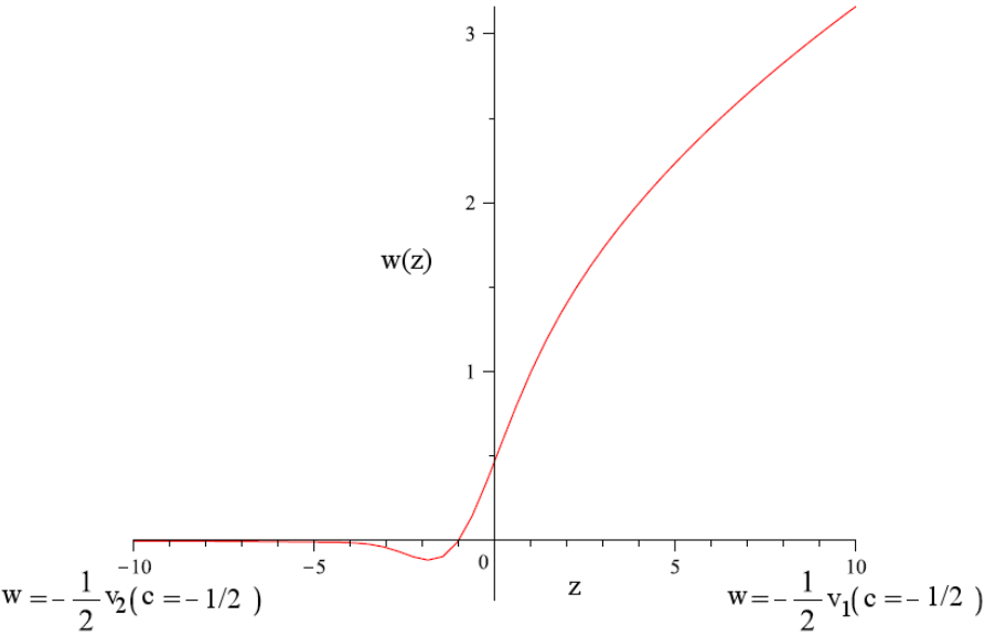
Refer to caption — Figure 1: A plot of the $k=2$ type 0A solution showing how the perturbative regimes at large $|z|$ are smoothly connected. Section 3 discusses a function $v(x)$ ( $x\propto z$ ), which has a number of different classes of behaviour distinguished by choice of boundary condition. The type 0A theory has class $v_{1}(z)$ in the $+z$ perturbative regime and class $v_{2}(z)$ in the $-z$ perturbative regime. Here we have set $\nu=1$ and $\Gamma=0$ .

As instructed in equation (6), integrating twice the asymptotic expansions (such as those in equations (9) and (10)) furnishes the free energy $F(\mu)$ , and it can be seen to define a perturbative expansion in the dimensionless string coupling

g_{s}=\frac{\nu}{\mu^{1+\frac{1}{2k}}}\quad.

(11)

For all models, in the $\mu\rightarrow+\infty$ regime, $\Gamma$ represents[12, 15] the number of background ZZ D–branes [25] in the model, with a factor of $\Gamma$ for each boundary in the worldsheet expansion. These are point–like branes localized at infinity in the Liouville direction $\phi$ , deep in the strong coupling region. In the $\mu\rightarrow-\infty$ regime, $\Gamma$ represents the number of units of RR–flux in the background, with $g_{s}^{2}\Gamma^{2}$ appearing when there is an insertion of pure RR–flux [15]. Since there is a unique non–perturbative solution connecting the two regimes, the string equation (1) supplies a non-perturbative completion of the theory that is a very clear example of a geometric transition between these two distinct (D-branes $vs$ RR–fluxes) spacetime descriptions of the physics.

The function $w(z)$ is the potential in the Hamiltonian ${\cal H}\equiv-\nu^{2}\partial^{2}_{z}+w(z)$ of the well–known (in the inverse scattering literature) associated Sturm–Liouville problem connected to the integrable KdV hierarchy. The wavefunctions of that problem define the partition functions of FZZT[26, 27] D–branes stretched along the Liouville direction $\phi$ , ending at a finite $\phi_{c}$ set by the eigenvalue. The zero–energy problem is interesting[20, 21], since there the FZZT D–branes stretch to infinity, and the Hamiltonian’s factorization, ${\cal H}=-(\nu\partial_{z}\pm g(z))(\nu\partial_{z}\mp g(z))$ where $w(z)=g(z)^{2}\pm g(z)^{\prime}$ , is highly convenient. The function $g(z)$ (its definition in the equation before is termed a Miura map in the integrable literature) satisfies[12] an infinite hierarchy of equations sometimes called the Painlevé II hierarchy since the equation at $k=1$ is the Painlevé II equation³³ 3 Those equations were derived in a string theory context by studying unitary matrix models[28, 29]. Painlevé II hierarchies have a mathematical life independent of this physical context, however. See e.g., refs[30, 31].. The asymptotic expansion of $y(z)$ generated by these equations is in terms of worldsheets involving ZZ D–branes (or fluxes) and FZZT D–branes. The entire problem defines a toy supersymmetric quantum mechanics problem within which the celebrated Bäcklund transformations of the KdV system can be made manifest. In this language the ZZ D–branes are identified with the number of threshold bound states (formally, zero–velocity solitons) of the system, and the Bäcklund transformations change their number by an integer. These more recently established features[20, 21], together with the earlier identification[23, 24] of the role of the KdV flows in organizing the close string operators, show how the integrable model and inverse–scattering technology of the mathematical physics literature comes to life in organizing the open and closed string content of minimal string theory.

2.2 Type 0B Strings

Type 0B string theory coupled to the $(2,4k)$ superconformal minimal models [15] is described succinctly by the following string equations[13, 14]:

\displaystyle\sum_{l=0}^{\infty}t_{l}(l+1)R_{l}=0\ ,\qquad\sum_{l=0}^{\infty}t_{l}(l+1)H_{l}+\nu q=0\ ,

(12)

where the $R_{l}$ and $H_{l}$ are polynomials of functions $r(x)$ and $\omega(x)$ (and their derivatives), and $\nu$ and $q$ are real constants.

The differential polynomials satisfy the following recursion relations

\displaystyle R_{l+1}=\omega R_{l}-\left(\frac{H_{l}^{\prime}}{r}\right)^{\prime}+rH_{l}\ ,\qquad H_{l+1}^{\prime}=\omega H_{l}^{\prime}-rR_{l}^{\prime}\ ,

(13)

where a prime denotes $\nu{\partial}/{\partial x}$ . Some of them are:

$\displaystyle H_{-1}$	$\displaystyle=$	$\displaystyle 1,\quad R_{-1}=0;$
$\displaystyle H_{0}$	$\displaystyle=$	$\displaystyle 0,\quad R_{0}=r;$
$\displaystyle H_{1}$	$\displaystyle=$	$\displaystyle-\frac{r^{2}}{2},\quad R_{1}=\omega r;$
$\displaystyle H_{2}$	$\displaystyle=$	$\displaystyle-r^{2}\omega,\quad R_{2}=-\frac{r^{3}}{2}+r\omega^{2}+r^{\prime\prime};$	(14)
$\displaystyle H_{3}$	$\displaystyle=$	$\displaystyle\frac{3}{8}r^{4}-\frac{3}{2}r^{2}\omega^{2}+\frac{1}{2}r^{\prime 2}-rr^{\prime\prime}\quad,$
$\displaystyle R_{3}$	$\displaystyle=$	$\displaystyle-\frac{3}{2}r^{3}\omega+r\omega^{3}+3r^{\prime}\omega^{\prime}+3\omega r^{\prime\prime}+r\omega^{\prime\prime}\quad.$

The function ${\widetilde{w}}(x)={r^{2}}/{4}$ defines the partition function of the theory $via$

{\widetilde{w}}(x)=\frac{r^{2}}{4}=\nu^{2}\frac{d^{2}F}{dx^{2}}\quad.

(15)

The $n$ th model is chosen by setting all $t_{l}$ to zero except $t_{0}\sim x$ and $t_{n}$ , analogous to what was done in the previous section concerning the 0A case. Note that these models have an interpretation as type 0B strings coupled to the $(2,2n)$ superconformal minimal models only for even⁴⁴ 4 For odd $n$ , lack of modular invariance of the partition function rules out the interpretation as type 0B strings coupled to superconformal matter [15]. $n$ . Writing $n=2k$ , we again have a set of models connected to the $(2,4k)$ superconformal minimal models, this time type 0B.

As in the 0A case, from the point of view of the $k$ th theory, all the other $t_{j}$ represent coupling to closed string operators $\mathcal{O}_{j}$ . Again the insertion of each operator can be expressed in terms of the Zakharov–Shabat[32] hierarchy of flows, the underlying integrable system in this case:

\displaystyle\frac{\partial\beta}{\partial t_{k}}=R_{k+1}\ ,\qquad\frac{\partial r}{\partial t_{k}}=-\frac{H^{{}^{\prime}}_{k+1}}{r}\ ,

(16)

where $\beta^{{}^{\prime}}\equiv\omega$ .

The asymptotic expansions of the string equations (12) for the first even $n=2k$ are:

$n=2\,\,\,(k=1)$

	$\displaystyle{\widetilde{w}}(x)$	$\displaystyle=$	$\displaystyle\frac{x}{4}+\left(q^{2}-\frac{1}{4}\right)\left[\frac{\nu^{2}}{2x^{2}}+\left(q^{2}-\frac{9}{4}\right)\left(\frac{-2\nu^{4}}{x^{5}}+\cdots\right)\right]\ ,\quad(x\rightarrow\infty)$
	$\displaystyle{\widetilde{w}}(x)$	$\displaystyle=$	$\displaystyle\frac{\nu q\sqrt{2}}{4\|x\|^{1/2}}-\frac{\nu^{2}q^{2}}{4\|x\|^{2}}+\frac{\nu^{3}}{\|x\|^{7/2}}\frac{5\sqrt{2}}{64}q\left(1+4q^{2}\right)+\cdots\quad(x\rightarrow-\infty)$		(17)

$n=4\,\,\,(k=2)$

	$\displaystyle{\widetilde{w}}(x)$	$\displaystyle=$	$\displaystyle\frac{\sqrt{x}}{4}+\frac{\nu^{2}}{144x^{2}}\left(64q^{2}-15\right)+\cdots;\quad(x\rightarrow\infty)$		(18)
	$\displaystyle{\widetilde{w}}(x)$	$\displaystyle=$	$\displaystyle\frac{\sqrt{\|x\|}}{2\sqrt{14}}+\frac{\nu}{2\|x\|^{3/4}}\frac{q}{\sqrt{3}\cdot 7^{1/4}}+\cdots\quad(x\rightarrow-\infty)$

Upon integrating twice, the asymptotic expansions in equations (17) and (18) furnish the free energy perturbatively as an expansion in the dimensionless string coupling, given by the same expression as before in equation (11).

For these models, in the $\mu\rightarrow-\infty$ regime, $q$ represents the number of background ZZ D–branes in the model, with a factor of $q$ for each boundary in the world sheet expansion, while in the $\mu\rightarrow\infty$ regime it counts the number of units of RR-flux in the background[15]. The asymptotic expansions in the two directions can be argued in ref.[15] to match onto each other analytically in a particular (’t Hooft) limit. For the case $k=1$ , the full non–perturbative solution is known since it can be mapped directly to the solution known for the $k=1$ type 0A case, as will be discussed below in section 2.3.

For later reference, we briefly discuss the structure of these solutions with increasing $n$ . As argued in ref.[15] the $n=2$ expansions are deformations of the solutions of the equation with $q=0$ . However things get interesting for $n=4$ . As before, the $x>0$ solution is a deformation of the solution with $q=0$ . For $x<0$ , $q=0$ allows for the trivial solution $r(x)=0$ , but trying to deform this for $q\neq 0$ leads only to a complex solution. Additionally, $q=0$ allows for two nontrivial solutions with $r(x)\neq 0$ and $\omega(x)\neq 0$ . These two are related by $\omega\rightarrow-\omega$ and are interpreted as $\IZ_{2}$ symmetry breaking solutions. In the interpretation of ref.[15], this is due to the presence of R–R fields. Both these solutions have a real extension to the case with $q\neq 0$ . The requirement of matching a $x<0$ solution to the $x>0$ solution picks out one of these for $q>0$ and the other for $q<0$ . (The $x<0$ solution listed above is for $q>0$ .) For higher $n$ , more such symmetry–breaking solutions arise. We will see how this is organized explicitly in section 6.

2.3 A Non–perturbative Connection Between 0A and 0B

It turns out that the simplest case of $n=2$ ( $k=1$ ), the 0A and 0B theories are non–perturbatively related in a very special way. In this case the conformal model is trivial (i.e. ${\hat{c}}=0$ ) and we simply have the pure world–sheet supergravity sector. The strings are unencumbered by a spacetime embedding (not counting the ubiquitous Liouville direction, $\phi$ ).

The string equation for the $k=1$ 0A theory, equation (1) with $\mathcal{R}=w(z)-z$ , is

w\left(w-z\right)^{2}-\frac{1}{2}\nu^{2}\frac{\partial^{2}w}{\partial z^{2}}\left(w-z\right)+\frac{1}{4}\nu^{2}\left(\frac{\partial w}{\partial z}-1\right)^{2}=\nu^{2}\Gamma^{2}\quad.

(19)

On the other hand, the string equation (12) for the $k=1$ 0B theory can be written succinctly as

\nu^{2}\frac{\partial^{2}r}{\partial x^{2}}-\frac{1}{2}r^{3}+\frac{1}{2}xr+\nu^{2}\frac{q^{2}}{r^{3}}=0\quad.

(20)

Notice that the perturbative expansion for the $k=1$ 0A theory as $z\rightarrow\infty$ (equation (9)) looks similar to the perturbative expansion for the $n=2$ 0B theory as $x\rightarrow-\infty$ (equation (17)) up to a (non–universal) sphere term, once one identifies $\Gamma$ with $q$ . The two expansions are just offset by various powers of $2$ . In fact there exists a non–perturbative map between the two equations [8, 33] that can be seen as follows. First define a function $f(z)$ via

w(z)=f(z)^{2}+z\quad,

(21)

for which the string equation for the 0A theory (19) becomes

\nu^{2}\partial^{2}_{z}f-f^{3}-zf+\nu^{2}\frac{\Gamma^{2}}{f^{3}}=0\quad.

(22)

After rescaling using

\displaystyle f=2^{-1/6}r;\qquad z=2^{-1/3}x\quad.

equation (22) becomes the string equation for the 0B theory (20), but with the sign of $x$ reversed. The physics of pure 0A supergravity and pure 0B supergravity (i.e. ${\hat{c}}=0$ ) are non–perturbatively related, with the brane and flux perturbative regions exchanged.

This non–perturbative connection between the 0A and 0B theories (for $k=1$ ) follows, mathematically, from the fact that the same basic string equation appears at the base of the two separate (KdV vs ZS) hierarchies of equations. This connection is partly in the spirit of a much larger set of connections that we are reporting on in this paper. We find that the KdV and ZS structures are embedded in a much larger structure, the dispersive water wave hierarchy of equations, and find a class of connections (of a different sort) between 0A and 0B for all $k$ and see that they define two special corners of a larger tapestry of physical theories.

3 The Dispersive Water Wave Hierarchy

The standard dispersive water wave (DWW) hierarchy[34], which will play a central role in the new physics we uncover, is a two--component system⁵⁵ 5 See refs.[35, 36, 37] for earlier studies of the properties of the dispersive water wave equations, and we will use the notation of refs.[34, 38].. It is described by:

\mathbf{u}_{t_{n}}=R^{n}\mathbf{u}_{x}\equiv\nu\partial_{x}\mathbf{L}_{n+1}[\mathbf{u}]\quad,

(23)

where $\mathbf{u}_{t_{n}}\equiv\partial_{t_{n}}\mathbf{u}$ , $\mathbf{u}_{x}\equiv\nu\partial_{x}\mathbf{u}$ (note that here and in the rest of the paper, for any function $G(x)$ , $G_{x}$ will denote $\nu\,\partial G/\partial x$ ), and we adopt a matrix notation:

\displaystyle\mathbf{u}=\left(\begin{array}[]{c}u\\ v\end{array}\right),\quad\quad\mathbf{L}_{n}[\mathbf{u}]=\left(\begin{array}[]{c}L_{n}[u,v]\\ K_{n}[u,v]\end{array}\right)\ .

Here,

R\equiv\frac{1}{2}\left(\begin{array}[]{cc}\partial_{x}u\partial_{x}^{-1}-\partial_{x}&2\\ 2v+v_{x}\partial_{x}^{-1}&u+\partial_{x}\end{array}\right)\quad,

(25)

is the recursion operator for the DWW hierarchy. The operator $R$ can be written as the quotient of two Hamiltonian operators $B_{1}$ and $B_{2}$ ,

\displaystyle R=B_{2}\circ B_{1}^{-1}\quad,

where $B_{1}$ and $B_{2}$ are given by

\displaystyle B_{2}=\frac{1}{2}\left(\begin{array}[]{cc}2\partial_{x}&\partial_{x}u-\partial_{x}^{2}\\ u\partial_{x}+\partial_{x}^{2}&v\partial_{x}+\partial_{x}v\end{array}\right)\ ,\qquad B_{1}=\left(\begin{array}[]{cc}0&\partial_{x}\\ \partial_{x}&0\end{array}\right)\ .

The $\mathbf{L}_{n}$ obey the recursion relation

\mathbf{L}_{n+1,x}=R\,\mathbf{L}_{n,x}\,,

(31)

which follows immediately from (23). The first few $L_{n}$ and $K_{n}$ are as follows:

$\displaystyle L_{0}$	$\displaystyle=$	$\displaystyle 2;\quad K_{0}=0;$
$\displaystyle L_{1}$	$\displaystyle=$	$\displaystyle u;\quad K_{1}=v;$
$\displaystyle L_{2}$	$\displaystyle=$	$\displaystyle\frac{1}{2}u^{2}+v-\frac{1}{2}u_{x};\quad K_{2}=uv+\frac{1}{2}v_{x};$
$\displaystyle L_{3}$	$\displaystyle=$	$\displaystyle\frac{1}{4}u^{3}+\frac{3}{2}uv-\frac{3}{4}uu_{x}+\frac{1}{4}u_{xx};$	(32)
$\displaystyle K_{3}$	$\displaystyle=$	$\displaystyle\frac{3}{4}u^{2}v+\frac{3}{4}v^{2}+\frac{3}{4}uv_{x}+\frac{1}{4}v_{xx}\quad.$

The normalization of $\mathbf{L}_{0}$ is chosen so as to reproduce (23) for $n=0$ .
The DWW hierarchy can be reduced to a one–component system by demanding that one of the two independent functions vanish. If we set $u(x)=0$ , we actually reduce to the KdV hierarchy: two operations of the (reduced) DWW recursion operator give

R\circ R\equiv R^{2}=\left(\begin{array}[]{cc}R_{2}&0\\ \frac{1}{4}(2v_{x}+v_{xx}\partial_{x}^{-1})&R_{2}\end{array}\right)\quad,

(33)

where $R_{2}=\frac{1}{4}(\partial_{x}^{2}+4v+2v_{x}\partial_{x}^{-1})$ is the recursion operator of the KdV hierarchy, shown in equation (3). Thus we obtain a reduction of the even flows of the original hierarchy (23) to

v_{t_{2n}}=R_{2}^{n}v_{x}\ ,

(34)

which is the KdV system in $-v(x)$ with independent variable $x$ , and the even times of DWW map to the times of the KdV $t_{2n}\to t_{n}$ . (Compare with equation (7)).
In addition, the recursion relation (31) reduces to

L_{2n+2,x}=R_{2}\circ L_{2n,x},

(35)

which is exactly the KdV recursion relation (3). The relative normalizations are $L_{0}=2$ and $P_{0}=\frac{1}{2}$ so we conclude that $L_{2n}=4P_{k}$ . Moreover, with $u=0$ , it is immediate that $L_{2n+1}=0$ .

The other obvious reduction, $v(x)=0$ , reduces the system to the Burgers hierarchy. We do not explore if there are any string theory consequences of that in this paper, since $v(x)$ is used to define the partition function of our theories in all our examples.

3.1 Scaling Reductions and New String Equations

Integrable hierarchies of partial differential equations (PDEs) can be reduced to ordinary differential equations (ODEs) through an additional condition on the variables. In our context, these ODEs are sometimes to be thought of as defining string theories; they are the “string equations” of a family of theories, forming an hierarchy themselves. As outlined around equation (7), string equations can be thought of as supplying the initial conditions for the partition function, and then the PDEs of flows describe how the partition function evolves as a function of the operators that couple to the $t_{k}$ [23]. The original example of all this[5, 6, 7] was a hierarchy of equations that have the Painlevé I equation as the non–trivial equation at their base, indexed by an integer $k$ . They defined the bosonic $c<1$ string theories coupled to the $(2,2k-1)$ conformal minimal models.

It was later realized[10] that another rich family of string equations (those in equations (1)) can be obtained by imposing certain scaling relations on the variables of the KdV system (note however that the equations were originally derived[8, 9] directly from matrix model constructions analogous to the original route). With this in mind, we explore a similarity reduction of the DWW hierarchy, expecting to obtain new string equations at the end of the day.

We follow the approach originally used to derive the string equations of type 0A (1) for the KdV hierarchy [10, 12]. To that end, assign $v$ mass dimension 1. The dimensions of the other terms uniquely follow from (23) and are $[u]=\frac{1}{2}$ , $[x]=-\frac{1}{2}$ and $[t_{n}]=-\frac{1}{2}(n+1)$ Thus we can write down two Callan–Symanzik equations expressing the scaling symmetry,

\begin{split}\frac{1}{2}u+\frac{1}{2}xu_{x}+\sum_{n=0}^{\infty}\frac{1}{2}(n+1)t_{n}u_{t_{n}}&=0\\ v+\frac{1}{2}xv_{x}+\sum_{n=0}^{\infty}\frac{1}{2}(n+1)t_{n}v_{t_{n}}&=0\quad.\end{split}

(36)

Using (23) and (31) we can rewrite these equations,

\begin{split}\frac{1}{2}u+\frac{1}{2}xu_{x}+\sum_{n=0}^{\infty}\frac{1}{2}(n+1)t_{n}\left(\frac{1}{2}uL_{n,x}+K_{n,x}-\frac{1}{2}L_{n,xx}+\frac{1}{2}u_{x}L_{n}\right)&=0\\ v+\frac{1}{2}xv_{x}+\sum_{n=0}^{\infty}\frac{1}{2}(n+1)t_{n}\left(\frac{1}{2}v_{x}L_{n}+\frac{1}{2}K_{n,xx}+\frac{1}{2}uK_{n,x}+vL_{n,x}\right)&=0\quad.\end{split}

(37)

Defining,

\left(\begin{array}[]{c}\mathcal{L}\\ \mathcal{K}\end{array}\right)=\sum_{n=0}^{\infty}\frac{1}{2}(n+1)t_{n}\mathbf{L}_{n},

(38)

we can rewrite (37),

	$\displaystyle\frac{1}{2}u\mathcal{L}_{x}+\frac{1}{2}u_{x}\mathcal{L}+\mathcal{K}_{x}-\frac{1}{2}\mathcal{L}_{xx}$	$\displaystyle=$	$\displaystyle 0$		(39)
	$\displaystyle v\mathcal{L}_{x}+\frac{1}{2}v_{x}\mathcal{L}+\frac{1}{2}\mathcal{K}_{xx}+\frac{1}{2}u\mathcal{K}_{x}$	$\displaystyle=$	$\displaystyle 0\quad,$		(40)

where we have used the fact that we will take $t_{0}=x$ and the other $t_{n}$ to be independent of $x$ . Equation (39) can readily be integrated. Moreover, solving (39) for $\mathcal{K}_{x}$ and substituting the result into (40) yields an expression, which, after multiplying by $\mathcal{L}$ , can also be integrated. The results are our new coupled string equations,

	$\displaystyle-\frac{1}{2}\mathcal{L}_{x}+\frac{1}{2}u\mathcal{L}+\mathcal{K}$	$\displaystyle=$	$\displaystyle\nu c\quad\quad\quad\quad\quad$		(41)
	$\displaystyle\left(-v+\frac{1}{4}u^{2}+\frac{1}{2}u_{x}\right)\mathcal{L}^{2}-\frac{1}{2}\mathcal{L}\mathcal{L}_{xx}+\frac{1}{4}\mathcal{L}_{x}^{2}$	$\displaystyle=$	$\displaystyle\nu^{2}\Gamma^{2}\quad,\quad\quad\quad\quad\quad$		(42)

where we have introduced two integration constants, $c$ and $\Gamma$ . We stress that the simplest possibility is for $c$ and $\Gamma$ to be independent of $x$ and $t_{i}$ , though only independence of $x$ is strictly necessary.
The $n$ th model is chosen by setting all $t_{i}$ equal to zero except for $t_{0}=x$ and $t_{n}$ which is chosen to be a numerical factor to fix the normalization. We choose to parameterize $t_{n}$ as

g_{n}\equiv\frac{1}{\frac{1}{2}(n+1)t_{n}}

(43)

in order to make direct contact with some recent literature which discusses this system in a much different (mathematical) context[38].

4 The Organizing Role of Painlevé IV

Let us focus on the case $n=1$ , which forms the bottom of the hierarchy of string equations from which all others follow using the recursion relations. The string equations in this case reduce to the Painlevé IV equation, an important equation from the mathematical literature. Its appearance at the bottom of the ladder of string equations we’re presenting here is significant. Note that the entire family of string equations can be generated from this $n=1$ case by use of the recursion operator, and so structures at this level will be reflected at higher $n$ , even while the complexity of the equations increases. Also notable is that this is the first time that a role for this equation has been uncovered in this context of non–perturbative string theory, and it takes its place alongside the Painlevé I and II equations whose roles (mentioned earlier) have been established in this context already. In fact, part of the motivation that led to the discoveries upon which we report here was the question as to the further role of the Painlevé equations in such systems. Painlevé IV emerged naturally as a candidate equation to play a role and this led to our studying of the DWW system that we found connected to Painlevé IV in the literature[38].

Let us see more explicitly how the equation emerges. Remarkably, it will naturally appear in two different ways[38, 39].

4.1 Painlevé IV: First Movement

The string equations for $n=1$ are:

	$\displaystyle 2v-u_{x}+u^{2}+g_{1}xu=2\nu g_{1}(c+\frac{1}{2})\quad,\hskip 85.35826pt$		(44)
	$\displaystyle\left(-v+\frac{1}{4}u^{2}+\frac{1}{2}u_{x}\right)(u+g_{1}x)^{2}-\frac{1}{2}u_{xx}(u+g_{1}x)+\frac{1}{4}\left(u_{x}+\nu g_{1}\right)^{2}=\nu^{2}g_{1}^{2}\Gamma^{2}\quad.$

where we have used the relation $g_{1}=\frac{1}{t_{1}}$ .

Solving the first of these for $v$ gives

v=\frac{1}{2}\left(u_{x}-u^{2}-g_{1}xu+2\nu g_{1}(c+\frac{1}{2})\right)\quad,

(45)

and substituting this into the second yields a second order ODE in $u$ which, under the change of variables

u(x)=y(x)-g_{1}x\quad

(46)

becomes

y_{xx}=\frac{1}{2}\frac{y_{x}^{2}}{y}+\frac{3}{2}y^{3}-2g_{1}xy^{2}+2\left[\left(\frac{g_{1}^{2}x^{2}}{4}\right)-\nu\alpha_{1}\right]y-\nu^{2}\frac{1}{2}\frac{\beta^{2}_{1}}{y}\quad.

(47)

$\alpha_{1}$ and $\beta_{1}$ are constants related to $c$ and $\Gamma$ in the DWW string equations through

\displaystyle\alpha_{1}=g_{1}(c+\frac{1}{2})\ ,\qquad\beta_{1}=\pm 2g_{1}\Gamma\ ,

(48)

Setting $g_{1}=-2$ , and dropping the subscripts on the constants, gives

\displaystyle y_{xx}=\frac{1}{2}\frac{y_{x}^{2}}{y}+\frac{3}{2}y^{3}+4xy^{2}+2\left(x^{2}-\nu\alpha\right)y-\nu^{2}\frac{1}{2}\frac{\beta^{2}}{y}\ ,

(49)

which is the fourth Painlevé equation $P_{IV}$ in standard form, and

\alpha=-(2c+1)\ ,\quad\beta=-8\Gamma^{2}\ .

(50)

We will see in the next section, specific constraints yielding the 0A and 0B theories that require $c=-\frac{1}{2}$ and $\Gamma=0$ respectively. Notably, these are precisely the values for which the constants $\alpha$ and $\beta$ in the standard form of Painlevé IV vanish.

4.2 Painlevé IV: Second Movement

In fact, there is another natural appearance of the Painlevé IV equation in this system[38, 39], at $n=1$ . There is a natural generalization[34] of the Miura map (that we saw for KdV in section 2) to the DWW system, defining new variables $U$ and $V$ :

u=U\ ,\qquad v=UV-V^{2}+V^{\prime}\ .

(51)

Now, as we saw above, $y(x)=u(x)-2x=U(x)-2x$ satisfies Painlevé IV with constants $\alpha$ and $\beta$ given in equation (49). Well, additionally, $-V(x)$ satisfies a copy of Painlevé IV (equation (49)) also, but with constants related to our physical parameters by

\alpha=\mp 3\Gamma+c+1\ ,\quad\beta=(c\pm\Gamma)^{2}\ .

(52)

We take this seriously, not the least because the variables described by the Miura map in the case of KdV (type 0A) were seen to be physically very natural, pertaining as they do to the FZZT and ZZ D–branes. (See the end of section 2.1 for a brief review.) We expect therefore (but this needs more exploration) that this DWW Miura map also leads to rich physics. The cases $c=\pm\Gamma$ and $c=-1\pm 3\Gamma$ imply vanishing of $\alpha$ and $\beta$ and may well have some special significance in this context. (We will, for example, find special solutions for all $n$ corresponding to $c=\pm\Gamma$ points. It is also interesting to note that the equations together point to the values $c=\pm\frac{1}{2}$ , $\Gamma=\pm\frac{1}{2}$ , values which do feature prominently in what is to follow.)

5 Connecting the Type 0 String Theories

Having introduced the DWW hierarchy, we now show how both the type 0A and type 0B string theories coupled to the $(2,4k)$ superconformal minimal models can be found embedded in this system. We show that by placing appropriate constraints on the full system of string equations, one can recover the respective string equations for both of the type 0 theories. Quite beautifully, these constraints require one of the two integration constants $(c,\Gamma)$ to freeze to particular values. The remaining unfixed constant then acts as the parameter that counts the number of ZZ–branes or units of R–R flux in each theory, depending on which asymptotic region (positive or negative large $x$ ) is under consideration.

5.1 Reduction to 0A

It was seen in section (3) that setting $u$ = $0$ reduces the DWW hierarchy to the KdV hierarchy. We therefore expect that this constraint also reduces our new string equations to the 0A string equations. That this indeed occurs can be seen as follows. Equation (38) gives,

\begin{split}\mathcal{L}[u\mathrm{=}0,v\mathrm{=}-w]&=\sum_{n=0}^{\infty}\frac{1}{2}(n+1)t_{n}^{\mathrm{DWW}}L_{n}\\ &=\sum_{n=0}^{\infty}\frac{1}{2}(2n+1)t_{2n}^{\mathrm{DWW}}L_{2n}\\ &=4\sum_{j=0}^{\infty}(j+\frac{1}{2})t_{2j}^{\mathrm{DWW}}P_{j}\\ &=\mathcal{R}[w]\end{split}

(53)

where we have used that $L_{2n+1}[u$ = $0,v]=0$ and $L_{2n}[u$ = $0,v$ = $-w]=4P_{n}[w]$ (see below (35)). The last equality holds provided that we make the identification,

t_{2n}^{DWW}=\frac{1}{4}t_{n}^{\mathrm{KdV}}=\frac{(-1)^{n+1}4^{n}(n!)^{2}}{(2n+1)!}\;\Rightarrow\;g_{2n}=2\frac{(-1)^{n+1}(2n)!}{4^{n}(n!)^{2}}\quad.

(54)

Finally, we see that when $u=0$ and $v=-w$ , equation (42) exactly reduces to equation (1), i.e. our new string equations encode 0A string theory coupled to the $(2,4k)$ superconformal minimal models. For even flows it is easy to show that $u=0$ is only consistent with the other string equation (41) if $c$ is frozen:

c=-\frac{1}{2}\ .

(55)

So one of the parameters in the original DWW equations becomes fixed when recovering type 0A coupled to the $(2,4k)$ superconformal minimal models, while the other parameter $\Gamma$ counts the number of branes or units of RR–flux in the type 0A theory. We will see this behaviour again in the case that we recover the type 0B theory.

5.2 Reduction to 0B

Consider the following redefinition of the DWW variables $\{u(x),v(x),x\}$ to the ZS variables $\{r(y),\omega(y),y\}$ :

\displaystyle y=2x,\quad u(y)=2\left(\omega(y)-\frac{r_{y}}{r(y)}\right),\quad v(y)=-r^{2}(y)\ .

(56)

The recursion relation (31) becomes,

\left(\begin{array}[]{c}L_{n+1}\\ K_{n+1,y}\end{array}\right)=\left(\begin{array}[]{c}(\omega-\frac{r_{y}}{r})L_{n}-L_{n,y}+K_{n,y}\\ -r(rL_{n}-\frac{K_{n,y}}{r})_{y}+\omega K_{n,y}\end{array}\right),

(57)

or,

\left(\begin{array}[]{c}R_{n+1}\\ H_{n+1,y}\end{array}\right)=\left(\begin{array}[]{c}\omega R_{n}-\left(\frac{H_{n,y}}{r}\right)_{y}+rH_{n,y}\\ -rR_{n,y}+\omega H_{n,y}\end{array}\right),

(58)

where we have defined,

R_{n}=\frac{1}{2}\left(rL_{n}-\frac{K_{n,y}}{r}\right),\quad\quad H_{n}=\frac{1}{2}K_{n}.

(59)

These are precisely the recursion relations of the ZS hierarchy (13). Moreover, the $H_{n}$ and $R_{n}$ just defined actually agree with those presented in (14). It suffices to check $n=0$ : from (32) we have $L_{0}=2$ and $K_{0}=0$ which imply $H_{0}=0$ and $R_{0}=r$ , as expected.
Finally, we may ask how we can produce the 0B string equations (12) from our new string equations (41) and (42). The answer turns out to be simple and elegant: all we must do is set

\mathcal{L}=0\quad.

(60)

Equation (41) then requires,

\sum_{n=0}^{\infty}t_{n}(n+1)H_{n}-\nu c=0\quad,

(61)

which further implies,

\sum_{n=0}^{\infty}t_{n}(n+1)R_{n}=0\quad.

(62)

The $t_{n}$ required here to consistently produce the equations of [15] are identical to the values we determined earlier (54). So, upon identifying $c=-q$ , we have exactly produced the 0B string equations.
Again notice how the consistency of our constraint $\mathcal{L}=0$ with (42) forces one of our parameters to vanish

\Gamma=0\quad,

(63)

leaving the parameter $c=-q$ to count the number of ZZ branes or RR–fluxes in the type 0B theory. Finally, we remark that the partition function of the 0B theory is determined via

\begin{split}F&=\frac{1}{\nu^{2}}\int d^{2}y\;\frac{r(y)^{2}}{4}\\ &=-\frac{1}{\nu^{2}}\int d^{2}x\;v(x)\end{split}

(64)

so that $-v(x)$ encodes the partition function for both 0A and 0B.

6 DWW Unconstrained — Beyond the Familiar

We have seen that constraining the DWW string equations (41) appropriately leads to the 0A and 0B theories (coupled to the superconformal $(2,4k)$ series), respectively. The constraints take the system with two free parameters $(c,\Gamma)$ and define two special points: 0A with $(c=-1/2,\Gamma$ free) and 0B with $(c$ free, $\Gamma{=}0)$ . We can also consider the fully unconstrained system with both parameters $(c,\Gamma)$ unfixed, and general $\{v(x),u(x)\}$ . Interestingly, we get multiple asymptotic expansions for the variable $v(x)$ . The structure of the equations and the corresponding asymptotic expansions gets richer as $n$ increases. Since in both cases, asymptotic expansions of $v(x)$ gave us, upon integrating twice, an expansion of a partition function for a string theory, we look again for it to define an interesting partition function in the new cases we will encounter. While this is an assumption, we shall see it bear fruit presently.

In this section we will first list the asymptotic expansions for the first few $n$ obtained from the corresponding string equations. We will explain the organizational rules we use to group these expansions into various classes. A careful analysis of the patterns we uncover in what follows allows us to extrapolate to higher $n$ and predict the structure of the expansions for any $n$ . We will see that a subset of these, when appropriately combined, reproduce the type 0 expansions that we have already encountered. In addition, we obtain completely new expansions which have not been presented in the literature before. Our key observation here is that these also resemble perturbative sectors of string theories (either with branes or fluxes present). We take these seriously as new string theories and our task after this section will be to identify what string theories they might be.

The number of expansions grows large as $n$ increases (we will see later that the number of expansions is $(n+1)^{2}$ ). To deal with this proliferation of expansions, we classify them into classes whose members are related to one another by simple symmetries. The classes themselves are distinguished by a number of salient features, many of which we explore in what follows. We choose to define the classes based on their behavior at order $\nu^{0}$ (this is equivalent to the leading behavior in $g_{s}^{-2}$ , the sphere level of closed string perturbation theory, as we will see later). Since DWW is a two component system, we must consider the leading behavior of both functions, $u$ and $v$ . We adopt the following classification scheme:

\begin{split}\textrm{Class 1:}\quad&u_{1}\sim 0,\quad\quad\;v_{1}\sim x^{2/n}\\ \textrm{Class 2:}\quad&u_{2}\sim 0,\quad\quad\;v_{2}\sim 0\\ \textrm{Class 3:}\quad&u_{3}\sim x^{1/n},\quad v_{3}\sim 0\\ \textrm{Class 4:}\quad&u_{4}\sim x^{1/n},\quad v_{4}\sim x^{2/n},\quad u_{4}^{2}/v_{4}\sim 1/4\\ \textrm{Class 5:}\quad&u_{5}\sim x^{1/n},\quad v_{5}\sim x^{2/n},\quad u_{5}^{2}/v_{5}\sim a\neq 1/4\\ \end{split}

(65)

We postpone the detailed study of $u$ to subsequent work. Here we mention its leading behavior only to complete the classification; in what follows, we focus exclusively on $v$ and its asymptotic expansions.

The details of sections 6.1–6.4, being a list of examples that we found instructive, might be a little dry on first reading and so the reader is encouraged to skip to section 6.5 for the general case.

6.1 $n=1$

The string equations for this case were already written in equations (44). Solving the first of these for $v$ gave equation (45), and substituting into the second yields a scalar second order ODE in $u(x)$ (equivalent to Painlevé IV), which can be used to produce the expansions. Asymptotic expansions for $u(x)$ can then be used to yield asymptotic expansions for $v(x)$ using equation (45).

We obtain three classes of expansions for $v(x)$ ,

$\displaystyle v_{2}$	$\displaystyle=$	$\displaystyle\frac{\nu^{2}}{x^{2}}(c^{2}-\Gamma^{2})\left(1-\frac{\nu}{g_{1}x^{2}}6c+\frac{\nu^{2}}{g_{1}^{2}x^{4}}(45c^{2}-5\Gamma^{2}+5)-\cdots\right)\quad,$
$\displaystyle v_{3}$	$\displaystyle=$	$\displaystyle\nu(c-\Gamma)\left(1-\frac{\nu}{g_{1}x^{2}}2\Gamma-\frac{\nu^{2}}{g_{1}^{2}x^{4}}6\Gamma(c-3\Gamma)-\cdots\right)\quad,$	(66)
$\displaystyle v_{4}$	$\displaystyle=$	$\displaystyle\frac{1}{9}g_{1}^{2}x^{2}+\nu\frac{2g_{1}c}{3}-\frac{\nu^{2}}{x^{2}}\frac{1}{3}(3c^{2}+9\Gamma^{2}-1)+\frac{\nu^{3}}{g_{1}x^{4}}6c(c^{2}-9\Gamma^{2})-\cdots\quad.$

Upon integrating twice (following what we learned from the type 0 theories in sections 2.1 and 2.2), one can obtain the free energy for a genus expansion of a string theory which allows us to identify the string coupling to be $g_{s}={\nu}/{x^{2}}$ .

6.1.1 Symmetries for $n=1$

The other expansions within each class can be obtained by the following symmetry operation:

\displaystyle f_{1}:\Gamma\to-\Gamma\quad.

Since $v_{2}$ and $v_{4}$ contain only even powers of $\Gamma$ , the are invariant under this map; however, $f_{1}\circ~v_{3}~\neq~v_{3}$ . Thus there are two expansions in the $v_{3}$ class, and, together with $v_{2}$ and $v_{4}$ , these comprise four total $n=1$ expansions.

6.2 $n=2$

The string equations are:

$\displaystyle u_{xx}$	$\displaystyle=$	$\displaystyle 3uu_{x}-u^{3}-6uv-2g_{2}xu+4\nu g_{2}\left(c+\frac{1}{2}\right)\quad,$
$\displaystyle v_{xx}$	$\displaystyle=$	$\displaystyle 2\left(\frac{(uv+\frac{1}{2}v_{x}-\nu g_{2}c)^{2}-\nu^{2}{g_{2}}^{2}{\Gamma}^{2}}{v+\frac{1}{2}u^{2}-\frac{1}{2}u_{x}+g_{2}x}\right)$	(67)
		$\displaystyle-2v\left(v+\frac{1}{2}u^{2}-\frac{1}{2}u_{x}+g_{2}x\right)-2(uv)_{x}\quad.$	(67)

where again $g_{2}=\frac{1}{t_{2}}$ . Solving the first of these for $v$ gives,

v=\frac{1}{6u}\left(u_{xx}-3uu_{x}+u^{3}+2g_{2}xu-4\nu g_{2}\left(c+\frac{1}{2}\right)\right)\quad.

(68)

Substituting this into the second yields a scalar fourth order ODE in $u$ , which can then be used to produce the expansions for $v$ . In this case, there are four relevant classes of expansions

$\displaystyle v_{1}$	$\displaystyle=$	$\displaystyle-g_{2}x-\frac{\nu g_{2}^{1/2}}{x^{1/2}}\Gamma+\frac{\nu^{2}}{x^{2}}\frac{1}{8}\left(-4c^{2}+4\Gamma^{2}+1\right)+\cdots\quad,$
$\displaystyle v_{2}$	$\displaystyle=$	$\displaystyle\frac{\nu^{2}}{x^{2}}\left(c^{2}-\Gamma^{2}\right)\left(1-\frac{2\nu^{2}}{g_{2}x^{3}}(5c^{2}-\Gamma^{2}+1)+\cdots\right)\quad,$	(69)
$\displaystyle v_{3}$	$\displaystyle=$	$\displaystyle\frac{g_{2}^{1/2}\nu}{x^{1/2}}(c-\Gamma)\left(\frac{i}{\sqrt{2}}+\frac{\nu}{g_{2}^{1/2}x^{3/2}}\frac{1}{4}(c-5\Gamma)-\cdots\right)\quad,$
$\displaystyle v_{4}$	$\displaystyle=$	$\displaystyle-\frac{g_{2}x}{5}+\frac{\nu g_{2}^{1/2}}{x^{1/2}}\frac{ic}{\sqrt{5}}-\frac{\nu^{2}}{x^{2}}\frac{1}{4}(2c^{2}+10\Gamma^{2}-1)-\cdots\quad.$

Here, we see that the string coupling is $g_{s}={\nu}/{x^{\frac{3}{2}}}$ .

6.2.1 Symmetries for $n=2$

The other expansions within each class can be obtained by the following operations,

\displaystyle f_{1}:\Gamma\to-\Gamma\ ,\qquad f_{2}:c\to-c\ ,

and compositions thereof. Some of the $v_{i}$ are invariant under one or both of these maps. Altogether, there are nine distinct expansions. Here are the four classes of expansions together with the number of distinct expansions within each class and the maps that lead to them:

\displaystyle v_{1}(2):\{1,f_{1}\};\quad v_{2}(1):\{1\};\quad v_{3}(4):\{1,f_{1},f_{2},f_{1}\circ f_{2}\};\quad v_{4}(2):\{1,f_{2}\}\quad.

6.3 $n=3$

The string equations are too long to be written down explicitly here and so we omit them. Four classes of expansions are produced in this case, and one sees expansions in Class 5 appearing for the first time here.

$\displaystyle v_{2}$	$\displaystyle=$	$\displaystyle\frac{\nu^{2}}{x^{2}}(c^{2}-\Gamma^{2})\left(1-\frac{\nu^{3}}{g_{3}x^{4}}\frac{5}{2}c(7c^{2}-3\Gamma^{2}+5)+\cdots\right)\quad,$
$\displaystyle v_{3}$	$\displaystyle=$	$\displaystyle\frac{\nu}{x^{2/3}}(c-\Gamma)\left(\frac{(-2)^{2/3}g_{3}^{1/3}}{3}+\frac{\nu}{x^{4/3}}\frac{1}{3}(c-3\Gamma)-\cdots\right)\quad,$	(70)
$\displaystyle v_{4}$	$\displaystyle=$	$\displaystyle\frac{2\cdot 2^{1/3}}{35^{2/3}}g_{3}^{2/3}x^{2/3}+\frac{\nu g_{3}^{1/3}}{x^{2/3}}\frac{2\cdot 2^{2/3}c}{3\cdot 35^{1/3}}-\frac{\nu^{2}}{x^{2}}\frac{1}{9}(3c^{2}+21\Gamma^{2}-2)+\cdots\quad,$
$\displaystyle v_{5}$	$\displaystyle=$	$\displaystyle-\frac{2\cdot 2^{1/3}}{5^{2/3}}g_{3}^{2/3}x^{2/3}-\frac{\nu g_{3}^{1/3}}{x^{2/3}}\frac{2^{2/3}}{3\cdot 5^{1/3}}(c+\sqrt{5}\Gamma)-\frac{\nu^{2}}{x^{2}}\frac{1}{9}(3c^{2}-3\Gamma^{2}-1)+\cdots\quad.$

Here the string coupling turns out to be $g_{s}={\nu}/{x^{\frac{4}{3}}}.$

6.3.1 Symmetries for $n=3$

The other expansions within each class can be obtained by the following operations,

f_{1}:\Gamma\to-\Gamma\ ,\quad f_{3}:x\to-x\ ,\quad f_{4}:g_{3}\to-g_{3}\ ,

(71)

and any compositions of these maps. A quick calculation shows that there 16 different expansions

$\displaystyle v_{2}(1)$	$\displaystyle:$	$\displaystyle\{1\};$
$\displaystyle v_{3}(6)$	$\displaystyle:$	$\displaystyle\{1,f_{1},f_{3}=f_{4},f_{1}\circ f_{3}=f_{1}\circ f_{4},f_{1}\circ f_{3}\circ f_{4},f_{3}\circ f_{4}\};$
$\displaystyle v_{4}(3)$	$\displaystyle:$	$\displaystyle\{1,f_{3}=f_{4},f_{3}\circ f_{4}\};$
$\displaystyle v_{5}(6)$	$\displaystyle:$	$\displaystyle\{1,f_{1},f_{3}=f_{4},f_{1}\circ f_{3}=f_{1}\circ f_{4},f_{1}\circ f_{3}\circ f_{4},f_{3}\circ f_{4}\}\quad.$

6.4 $n=4$

Our explicit string equations are rather complicated and so we will not list them here. The following five classes of expansions are obtained:

$\displaystyle v_{1}(x)$	$\displaystyle=$	$\displaystyle-\frac{2i}{\sqrt{3}}\sqrt{g_{4}}\sqrt{x}-\frac{\nu g_{4}^{1/4}}{x^{3/4}}\frac{(1+i)\Gamma}{2\cdot 3^{1/4}}-\frac{\nu^{2}}{x^{2}}\frac{1}{48}\left(12c^{2}-12\Gamma^{2}-5\right)+\cdots\quad,$
$\displaystyle v_{2}(x)$	$\displaystyle=$	$\displaystyle-\frac{\nu^{2}}{x^{2}}(\Gamma^{2}-c^{2})\left(1-\frac{3\nu^{4}}{2g_{4}x^{5}}(21c^{4}-14c^{2}\Gamma^{2}+\Gamma^{4}+35c^{2}-5\Gamma^{2}+4)\right)+\cdots\quad,$
$\displaystyle v_{3}(x)$	$\displaystyle=$	$\displaystyle-\frac{g_{4}^{1/4}\nu}{x^{3/4}}(c-\Gamma)\left(\frac{1}{2^{3/4}(1+i)}+\frac{\nu}{g_{4}^{1/4}x^{5/4}}\frac{7\Gamma-3c}{8}+\cdots\right)\quad,$	(72)
$\displaystyle v_{4}(x)$	$\displaystyle=$	$\displaystyle-\frac{2i}{3\sqrt{7}}\sqrt{g_{4}}\sqrt{x}-\frac{g_{4}^{1/4}\nu}{x^{3/4}}\frac{c}{\sqrt{3}\cdot 7^{1/4}(1+i)}-\frac{\nu^{2}}{x^{2}}\frac{1}{24}\left(6c^{2}+54\Gamma^{2}-5\right)+\cdots\quad,$
$\displaystyle v_{5}(x)$	$\displaystyle=$	$\displaystyle-2\sqrt{\frac{2}{21}}\sqrt{g_{4}}\sqrt{x}-\frac{g_{4}^{1/4}\nu}{x^{3/4}}\frac{21^{1/4}}{2^{5/4}}\left(-\frac{c}{\sqrt{7}}+\frac{\Gamma}{\sqrt{3}}\right)-\frac{\nu^{2}}{x^{2}}\frac{1}{48}\left(12c^{2}-12\Gamma^{2}-5\right)+\cdots\quad.$

Here, the string coupling is $g_{s}={\nu}/{x^{\frac{5}{4}}}$ .

6.4.1 Symmetries for $n=4$

The other expansions within each class can be obtained by the following operations,

f_{1}:\Gamma\to-\Gamma\ ,\quad f_{2}:c\to-c\ ,\quad f_{3,4}:(x,g_{4})\to(-x,-g_{4})\ ,

(73)

and any arbitrary composition of those maps. A quick calculation shows that there are 25 distinct expansions. Here are the five classes of expansions together with the number of distinct expansions within each class and the maps that lead to them:

$\displaystyle v_{1}(4)$	$\displaystyle:$	$\displaystyle\{1,f_{1},f_{3,4},f_{1}\circ f_{3,4}\};$
$\displaystyle\quad v_{2}(1)$	$\displaystyle:$	$\displaystyle\{1\};$
$\displaystyle\quad v_{3}(8)$	$\displaystyle:$	$\displaystyle\{1,f_{1},f_{2},f_{1}\circ f_{2},f_{3,4},f_{1}\circ f_{3,4},f_{2}\circ f_{3,4},f_{1}\circ f_{2}\circ f_{3,4}\};$
$\displaystyle v_{4}(4)$	$\displaystyle:$	$\displaystyle\{1,f_{2},f_{3,4},f_{2}\circ f_{3.4}\};$
$\displaystyle\quad v_{5}(8)$	$\displaystyle:$	$\displaystyle\{1,f_{1},f_{2},f_{1}\circ f_{2},f_{3,4},f_{1}\circ f_{3,4},f_{2}\circ f_{3,4},f_{1}\circ f_{2}\circ f_{3,4}\}\quad.$

6.5 Patterns and Asymptotia

The expansions displayed above for $n=1$ to $n=4$ exhibit a rich structure which we explore shortly. First we briefly review the interpretation given to the parameter $\Gamma$ of the 0A theory (and also to $q$ of the 0B theory). In the $\mu$ (or $x$ ) $\rightarrow+\infty$ regime, $\Gamma$ represents the number of background ZZ D–branes in the model, with a factor of $\Gamma$ for each boundary in the worldsheet expansion. Since an orientable surface with odd (even) Euler characteristic must contain an odd (even) number of boundaries, $\Gamma$ must be raised to an odd (even) power if $g_{s}$ is. In addition, the power of $\Gamma$ must be less than or equal to the power of $g_{s}$ . On the other hand, in the $\mu$ (or $x$ ) $\rightarrow-\infty$ regime, $\Gamma$ represents the number of units of RR–flux in the background, with $g_{s}^{2}\Gamma^{2}$ appearing when there is an insertion of pure RR–flux. So in this case both $\Gamma$ and $g_{s}$ should appear with even powers.
In applying these observations to our DWW expansions, we immediately notice the remarkable fact that the various expansions have powers of the parameters which somehow allow for interpretations as counting branes or fluxes. This is by no means guaranteed, and indeed its occurrence was one of our main motivations for in–depth study of the system. The presence of two parameters, however, leads to a few subtleties. For example, in some expansions an interpretation in terms of branes is only possible if one of the two parameters is set to zero. With keep such observations in mind as we begin the study of the various expansions.

Finally we note that the asymptotic direction (i.e., positive or negative $x$ ) of each expansion can be fixed by requiring that once we fix the value of $g_{n}$ , the expansion must be real (which is an important constraint since $v$ encodes the free energy). The value of $g_{n}$ , in turn, can be fixed using the values listed in equation (54) since we must reproduce the 0A theory. With all of these observations we are ready to begin analyzing our expansions.

6.5.1 Class 1

•

$v_{1}$ contains powers of $\Gamma$ consistent with those of a parameter counting branes. This remains true for any value of $c$ .
•

$v_{1}$ contains powers of $c$ consistent with those of a parameter counting fluxes. However, for arbitrary $\Gamma$ , $g_{s}$ appears with odd powers, inconsistent with our requirements for a description of fluxes, as mentioned above. This problem is avoided if we set $\Gamma=0$ since this forces the odd powers of $g_{s}$ to vanish.
•

In particular, setting $\Gamma=0$ with $g_{n}$ given by equation (54) reduces this expansion to the $x>0$ flux-expansion in $c$ (or $q$ ) for the type 0B theory seen in equations (17,18) for $n=2,4$ respectively.
•

Alternatively, setting $c=-\frac{1}{2}$ with the same value of $g_{n}$ reduces these expansions to those of the type 0A for $x>0$ . (We listed them in equations (9 and 10) for $k=1,2$ respectively⁶⁶ 6 Recall that the DWW hierarchy index $n$ is related to KdV hierarchy index $k$ by $n=2k$ ..)
•

With the values of $g_{n}$ need to reduce to 0A and 0B, one obtains real expansions in this class only if $x>0$ . Hence we fix this class of expansions to be $x\rightarrow+\infty$ asymptotic expansions.
•

This class of expansions only exists for even $n$ .

6.5.2 Class 2

•

For even $n$ , $v_{2}$ contains powers of $\Gamma$ and $g_{s}$ consistent with those of a parameter counting fluxes. This is true for all values of $c$ . For odd $n$ , the powers of $\Gamma$ are still consistent with the flux interpretation, but there are odd powers of $g_{s}$ which are inconsistent with fluxes. These odd powers can be removed by setting $c=0$ .
•

For even $n$ , $v_{2}$ contains powers of $c$ and $g_{s}$ consistent with a parameter counting fluxes. This is true for all values of $\Gamma$ . For odd $n$ , the powers of $c$ are consistent with those of a parameter counting branes. In this interpretation, there are no contributions from surfaces with only one boundary.
•

Setting $c=-\frac{1}{2}$ with $g_{n}$ as chosen in equation (54), reduces the $v_{2}$ expansions to the type 0A expansions for $x<0$ . (We listed them in equations (9) and (10) for $k=1,2$ respectively.)
•

Only even powers of $g_{n}$ and $x$ appear, so the requirement of reality does not fix the direction of these expansions.
•

Consistency with the 0A expansions forces us to consider the expansions in this class as $x\rightarrow-\infty$ expansions. We note the possibility that these might appear as $x\rightarrow+\infty$ expansions outside of the simple type 0A context we’ve seen so far⁷⁷ 7 In fact, we can already think of an example. There are rational solutions of the type 0A string equations that were considered in a string theory context in ref.[40]. The rational solutions have $v_{2}$ type expansions (for $c=-1/2$ ) in both asymptotic directions for $x$ . Clearly there are analogous rational solutions for the full DWW equations that have $v_{2}$ asymptotic expansions that generalize the known cases. We have constructed large families of them, and leave their study for a later publication..
•

These expansions vanish when $c^{2}=\Gamma^{2}$ . (This is a likely special point(s) in parameter space. We got a first hint of this point in section 4 where the second copy of Painlevé IV has $\beta=0$ .)
•

This class of expansions appears for all $n$ .

6.5.3 Class 3

•

$v_{3}$ contains powers of $\Gamma$ consistent with those of a parameter counting branes. This is true only for $c=0$ .
•

$v_{3}$ contains powers of $c$ consistent with those of a parameter counting branes. This is true only for $\Gamma=0$ .
•

We notice that associating one boundary to each factor of $c$ and $\Gamma$ also produces a consistent worldsheet expansion. We might speculate about whether, in general, these expansions might capture $c$ and $\Gamma$ simultaneously counting branes.
•

Setting $\Gamma=0$ with $g_{2}=1$ reduces these expansions to the $x<0$ brane-expansions for the type 0B theory for $n=2$ as seen in equation (17). Hence we fix the expansions in this class to be $x\rightarrow-\infty$ expansions.
•

At $n=4$ , the value $g_{4}=-\frac{3}{4}$ with $\Gamma=0$ renders this expansion complex for $x<0$ . This fits in nicely with the structure of expansions observed in the 0B case, reviewed⁸⁸ 8 Recall that the trivial solution with $r(x)=0$ in that case did not have a real deformation for $q\neq 0$ . The $v_{3}$ class is exactly the analogue of this trivial solution. in section 2.2.
•

$c=\Gamma$ causes these expansions to vanish (we got a first hint of this point in section 4 where the second copy of Painlevé IV has $\beta=0$ .)
•

This class of expansions exists for all $n$ , but is real as an $x<0$ expansion only for $n=2$ mod $4$ .

6.5.4 Class 4

•

The $v_{4}$ class of expansions has not, to our knowledge, made a previous appearance in the literature, as it does not appear until encountering the DWW system.
•

$v_{4}$ contains powers of $c$ consistent with those of a parameter counting branes. This remains true for any value of $\Gamma$ .
•

$v_{4}$ contains powers of $\Gamma$ consistent with those of a parameter counting fluxes. However, for arbitrary $c$ , $g_{s}$ appears with odd powers, inconsistent with our requirements for a description of fluxes, as mentioned above. This problem is avoided if we set $c=0$ since this forces the odd powers of $g_{s}$ to vanish.
•

The direction of $v_{4}$ is not immediately determined by the consistency conditions we have used so far. Compatibility with the type 0 theories at $n=2$ requires $g_{2}=1$ which renders $v_{4}$ real for $x\rightarrow-\infty$ . On the other hand, compatibility with the type 0 theories at $n=4$ requires $g_{4}=-\frac{3}{4}$ which renders $v_{4}$ real for $x\rightarrow+\infty$ .
•

We will later provide evidence in favor of $v_{4}$ existing for $x>0$ .
•

In general, for the type 0 choices (54) for $g_{n}$ , $v_{4}$ remains real for $x>0$ when $n=0$ mod $4$ and becomes complex when $n=2$ mod $4$ .
•

In the special case $n=2$ , $v_{4}$ can be made real by setting $c=0$ .

6.5.5 Class 5

•

$v_{5}$ contains powers of $\Gamma$ consistent with those of a parameter counting branes. This is true only for $c=0$ .
•

$v_{5}$ contains powers of $c$ consistent with those of a parameter counting branes. This is true only for $\Gamma=0$ .
•

As for $v_{3}$ , we notice that associating one boundary to each factor of $c$ and $\Gamma$ also produces a consistent worldsheet expansion. We might speculate that, in general, these expansions might capture $c$ and $\Gamma$ simultaneously counting branes.
•

These expansions do not exist for $n<3$ .
•

With $\Gamma=0$ and $g_{4}=-\frac{3}{4}$ this class reduces to the $x<0$ brane–expansion in $c$ seen for the 0B theory at $n=4$ in equation (18). (Recall that there $q=-c$ .)
•

These are the non–trivial broken–symmetry solutions obtained in the 0B theory as one increases $n$ . We reviewed this at the end of section 2.2.
•

As $n$ increases, further expansions in this class arise for every odd $n$ , which we generically label $v_{i\geq 5}$ . These are distinguished by the different values of $a$ in (65), but since their behavior is identical for our purposes we often group them together.
•

For odd $n$ , reality imposes no restrictions on the direction of $v_{i\geq 5}$ .
•

For $n=4$ , reality requires that we fix $v_{5}$ to be an $x\rightarrow-\infty$ expansion. For the subsequent even $n$ , some of the $v_{i\geq 5}$ are real for $+x$ , while the remaining are real for $-x$ .

6.6 The Structure at Higher $n$

We can extrapolate the pattern observed for the first few $n$ and make predictions for the structures that should appear at higher $n$ . The first observation is that there are $(n+1)^{2}$ expansions in all (taking into account the various expansions related by symmetries in each class) at each $n$ . The counting can be broken down as follows.

	$v_{2}$	$v_{4}$	$v_{1}$	$v_{3}$	$v_{5}$	$v_{6}$	$v_{7}$	${\rm total}$
$n=1$	1	1		2				4
$n=2$	1	2	2	4				9
$n=3$	1	3		6	6			16
$n=4$	1	4	4	8	8			25
$n=5$	1	5		10	10	10		36
$n=6$	1	6	6	12	12	12		49
$n=7$	1	7		14	14	14	14	64
$n=8$	1	8	8	16	16	16	16	81

Table 1: The number and types of expansion classes for

v(x)

, as a solution to the string equations (41) and (42), with increasing

n

from 1 to 8. See text for further discussion.

Class 2 has exactly one member for each $n$ , while Class 1 and Class 4 each have $n$ members. (Recall that Class 1 only exists for even $n$ .) As previously mentioned, for every odd $n$ , new expansions in Class 5 (the $v_{i\geq 5}$ ) appear. These reduce to the $x<0$ broken symmetry expansions of the 0B theory (for $\Gamma=0$ and $g_{n}$ in equation (54)) when $n$ is even. These expansion classes each contain $2n$ members. The appearance of these new expansions is consistent with the counting provided in ref.[15] for the 0B expansions, as reviewed at the end of section 2.2. The counting is tabulated in Table 1. All together, we see that for odd $n$ , adding across the rows gives a total of $1+n+\frac{n+1}{2}\cdot 2n=(n+1)^{2}$ expansions, while for even $n$ we get $1+n+n+\frac{n}{2}\cdot 2n=(n+1)^{2}$ expansions.

7 An Organizing Square

To construct a full solution for $v(x)$ , we need to specify its behaviour in the two asymptotic directions, positive and negative $x$ . Consider the example of type 0A discussed in section 2.1. The string equation at a given $k$ was shown to have a solution connecting these two perturbative regimes with a full non–perturbative completion, plotted for $k=2$ in figure 1. (Recall that $z\propto x$ and $w=-v$ .) This solution is in fact made of two expansions, $v_{1}(x)$ for the positive $x$ regime and $v_{2}(x)$ for negative $x$ . The parameter $c$ is frozen to $-\frac{1}{2}$ in this case, leaving the parameter $\Gamma$ to count D–branes at $+x$ and fluxes at $-x$ , as described in 6.5.

This is the organizing scheme we follow in order to construct more theories, with type 0B being another working example, this time with $\Gamma=0$ and using $v_{1}$ for positive $x$ and $v_{3},v_{5}$ , or the higher $v_{i}$ (not $v_{4}$ ) for negative $x$ , as already discussed.

In constructing new theories, matching perturbative expansions does not guarantee that a full non–perturbative solution exists with the desired properties. Further work is needed, using both analytic and numerical techniques, in order to demonstrate the non–perturbative existence of the proposed theories. This is the subject of our companion paper, where we find several non–perturbative solutions numerically, and present analytical arguments in favour of several new non–perturbatively complete theories. For the rest of this paper, our analysis will be concerned with the various perturbative regimes that appear from our DWW string equations.

Much of this structure can be organized neatly into the shape of a square, with the string theory special points we know so far at two of the corners. The $v_{1}$ and $v_{2}$ pair form two edges with the type 0A (with $c=-\frac{1}{2}$ ) theory where they join. Then $v_{3}$ (at $n=2$ ) (or $v_{5}$ at $n=4$ , and so on) make another edge, with type 0B ( $\Gamma=0$ ) at the corner where that edge meets the $v_{1}$ edge. See figure 2.

Using our observations from section (6.5), we conjecture that $v_{4}$ and $v_{2}$ form a physical pair when $\Gamma$ is fixed, with $c$ counting either branes of fluxes in the perturbative regimes. Similarly, $v_{4}$ with $v_{3}$ (or $v_{i\geq 5}$ ) may form physical pair for fixed $c$ , with $\Gamma$ counting fluxes or branes. Since $v_{2},v_{3}$ , and $v_{i\geq 5}$ appeared as $x<0$ expansions, it is natural to fix the direction of $v_{4}$ to be $+x$ . It fits elegantly at the bottom of the square, at least when $n=0\mod 4$ , (i.e., when $v_{4}$ is real for positive $x$ ).

We summarize all of this in figure 2. The special points in parameter space with $c^{2}=\Gamma^{2}$ or $c=\Gamma$ , where $v_{2}$ and $v_{3}$ vanish, are represented by the dark squares on the vertical edges.

This way of organizing things immediately suggests that there are two new special points, corresponding to the lower two corners of the square, and we’ve called them Theory A and Theory B. We will need to determine what the special values of $c$ and $\Gamma$ might be for these corners, and the nature of the new theories. (The special values $c=0$ and $\Gamma^{2}=\frac{1}{4}$ , complementary to the known values for the type 0 theories, are suggestive, but so far this is a guess. We will find several pieces of evidence to support this suggestion in later sections.)

The lines connecting the special points are not (at this stage) to be taken too literally, since we do not have a clear statement of the nature of the theory (stringy or not) away from the special points. However, the structure is highly suggestive, and reminiscent of the square discovered in ref.[17] organizing the moduli space of ${\hat{c}}=1$ strings. We reproduce it here in figure 3. ${\hat{c}}=1$ strings are fully two dimensional, having in addition to the Liouville direction $\phi$ an extra direction $X$ . This direction can be compactified on a circle, and in the square the lines represent values of radii varying between 0 and $\infty$ . The relations between theories then arise as a result of T–dualities (horizontally) possibly combined with discrete twists by discrete fermionic symmetry operations (vertically).

In the case under study here, there is generically no compact circle, and so the analogy is limited, but it is possible that it is not entirely coincidental that a square emerges. Two dimensional string theories can descend to ${\hat{c}}<1$ theories by Renormalization Group flow[18, 19], and so an organizing square at ${\hat{c}}=1$ may well leave an imprint at ${\hat{c}}<1$ that still is an organizing square. The fact that there are two special points on the vertical lines on the ${\hat{c}}=1$ square that match our $c^{2}=\Gamma^{2}$ and $c=\Gamma$ points is suggestive.

Inspired by the similarity between our square and that of ref.[17], we explored whether the two unknown theories at the bottom of our square could actually be type IIA and type IIB string theories, coupled to superconformal minimal models. We present the details of our explorations in section 8.

8 A Search for New Theories

So far, we have demonstrated that the DWW hierarchy has an extremely rich structure of asymptotic expansions that naturally contain both the 0A and 0B string theories coupled to the $(A,A)$ $(2,4k)$ superconformal minimal models. We’ve also pointed out that there are new expansions that seem to have perfectly stringy interpretations, in terms of backgrounds containing D–branes or fluxes once either $c$ or $\Gamma$ has been fixed. It is natural to wonder whether a sensible interpretation as string theories coupled to some matter minimal (super–minimal) models can be given to these new expansions. We will find some success with this for some corners of parameter space.

The square in figure 3 motivates the conjecture that the new string theories are type II string theories coupled to some superconformal minimal models. This has some physical motivation since type II string theories can be obtained as twisted orbifolds of type 0 theories. Also, the $(A,D)$ series of superconformal minimal models can be obtained as orbifolds of the $(A,A)$ series $via$ a twist in the matter sector. In descending from ${\hat{c}}=1$ to ${\hat{c}}<1$ , the remnants of the twisted T–dualities connecting the type 0 and type II sectors could well be a combination of these orbifold actions. In what follows, we argue that type II string theories coupled to $(A,D)$ $(4,4k-2)$ superconformal minimal models are natural candidates for the physics encoded by the new special points of our string equations.

One method of partially checking which theories are being captured by our asymptotic expansions is to compare the (putative) torus contributions (terms at order $g_{s}^{0}$ in the free energy) with a continuum calculation (i.e., results of a traditional world–sheet string one–loop computation) for these models. Such a comparison will enable us to specialize to various points in parameter space and provide further consistency checks to determine the exact underlying models.

8.1 The $g_{s}^{0}$ terms

We begin by listing the terms that appear at order $g_{s}^{0}$ in the expansion for the free energy for each class of the expansions studied in section 6, for all $n$ :

$\displaystyle v_{1}(x)$	$\displaystyle:$	$\displaystyle\frac{n+1}{12n}-\frac{c^{2}}{n}+\frac{\Gamma^{2}}{n}\quad,$
$\displaystyle v_{2}(x)$	$\displaystyle:$	$\displaystyle c^{2}-\Gamma^{2}\quad,$
$\displaystyle v_{3}(x)$	$\displaystyle:$	$\displaystyle\frac{n-1}{2n}c^{2}-\frac{n+1}{n}c\Gamma+\frac{n+3}{2n}\Gamma^{2}\quad,$	(74)
$\displaystyle v_{4}(x)$	$\displaystyle:$	$\displaystyle\frac{n+1}{6n}-\frac{c^{2}}{n}-\frac{2n+1}{n}\Gamma^{2}\quad,$
$\displaystyle v_{i}(x)$	$\displaystyle:$	$\displaystyle\frac{n+1}{12n}-\frac{c^{2}}{n}+\frac{\Gamma^{2}}{n}\quad,\quad(i\geq 5)\ .$

Notice that the torus term in the expansion classes labeled $v_{i}$ is identical to that in $v_{1}$ . This is a generalization of the curious observation that was made in ref.[15], that the symmetry breaking solutions (for $x<0$ ) of the 0B theory have the same torus terms (for $x>0$ ) as those of the 0B theory.

In each case, these terms are at order $x^{-2}$ in the expansion, and multiplied by $\nu^{2}$ . Following e.g., equations (6) and (15), the free energy is obtained by integrating twice and dividing by $\nu^{2}$ , yielding the same terms above multiplied by $\ln(|x|)$ , which is part of a standard Liouville theory volume factor that is common to everything we will do at this order at perturbation theory⁹⁹ 9 The Liouville direction $\phi$ is effectively a box of volume $V_{\rm L}=-\ln(|\mu|/\Lambda)/\alpha_{\rm min}$ where $\alpha_{\rm min}$ is the Liouville dressing of the lowest dimension operator in the theory (see e.g., refs.[42, 43] for a review). In a unitary theory, $\mu$ is the cosmological constant, the coefficient of the puncture operator, which measures worldsheet area. Recall that the dilaton and hence the local string coupling increases with $\phi$ , and so there is a natural cutoff at the point where perturbation theory begins to break down, denoted $\Lambda$ . Standard conventions are to choose a scale such that $\Lambda$ is unity and we will write $\mu=x$ in much of what follows, differing slightly from our notation in e.g., equation (6)..

8.2 The Continuum Partition Functions

We now present several continuum partition functions in the even spin structures sector for both type 0 and type II theories coupled to $(A,A)$ and $(A,D)$ modular invariants. Ref. [44], presents the modular invariant partition functions in the even spin structures $(-,-)$ , $(-,+)$ and $(+,-)$ for all the ${\cal{N}}=1$ superconformal minimal models, as classified in ref. [45]. Ref. [46] combines these results with Liouville theory to compute some of the string theory partition functions and we follow their methods to present the type II expressions that we suggest at the end of this section.

8.2.1 The Type 0 Theories

$\bullet$ The $(A_{p-1},A_{q-1})$ modular invariants.
The contribution of the even spin structures to the genus one path integral for the $(A_{p-1},A_{q-1})$ superconformal minimal models coupled to supergravity has been calculated in ref.[46]:

	$\displaystyle Z^{(A,A)}_{\rm even}$	$\displaystyle=$	$\displaystyle-\frac{1}{16}\frac{(p-1)(q-1)}{(p+q-1)}\ln\|x\|\quad,\quad(p,q\quad{\rm odd})$		(75)
	$\displaystyle Z^{(A,A)}_{\rm even}$	$\displaystyle=$	$\displaystyle-\frac{1}{16}\frac{(p-1)(q-1)+1}{(p+q-2)}\ln\|x\|\quad.\quad(p,q\quad{\rm even})$		(76)

$\bullet$ The $(A_{p-1},D_{q/2+1})$ modular invariants.
The superconformal minimal model partition functions may be written in terms of the partition functions for fields on a circle at special radii, as shown in ref.[44]. These can be combined with partition functions for affinized compact circle theories to yield the desired one–loop string theory expressions[46]. Using this technique, it is easy to show that the partition functions in the even spin structures for the $(A_{p-1},D_{q/2+1})$ modular invariants are:

	$\displaystyle Z^{(A,D)}_{\rm even}$	$\displaystyle=$	$\displaystyle-\frac{1}{64}\frac{(3p-4)(q+2)}{(p+q-2)}\ln\|x\|\ ,\quad(q=2\mod 4)\ ,$		(77)
	$\displaystyle Z^{(A,D)}_{\rm even}$	$\displaystyle=$	$\displaystyle-\frac{1}{32}\frac{(p-2)(q+3)+2}{(p+q-2)}\ln\|x\|\ ,\quad(q=0\mod 4)\ .$		(78)

8.2.2 The Type II Theories

By analogy with the previous section, similar procedures can be used to propose partition functions in the even spin structures for superconformal minimal models coupled to the type II string theories, using as starting point the partition functions for the corresponding circle theories given in ref.[17]. Our results are:

$\bullet$ The $(A_{p-1},A_{q-1})$ modular invariants.

	$\displaystyle\tilde{Z}^{(A,A)}_{\rm even}$	$\displaystyle=$	$\displaystyle\frac{1}{32}\frac{(p-1)(q-1)}{(p+q-1)}\ln\|x\|\quad,\quad(p,q\quad{\rm odd})$		(79)
	$\displaystyle\tilde{Z}^{(A,A)}_{\rm even}$	$\displaystyle=$	$\displaystyle\frac{1}{32}\frac{(p-1)(q-1)+1}{(p+q-2)}\ln\|x\|\quad.\quad(p,q\quad{\rm even})$		(80)

$\bullet$ The $(A_{p-1},D_{q/2+1})$ modular invariants.

	$\displaystyle\tilde{Z}^{(A,D)}_{\rm even}$	$\displaystyle=$	$\displaystyle\frac{1}{64}\frac{p(q+2)}{(p+q-2)}\ln\|x\|\ ,\quad(q=2\mod 4)\ ,$		(81)
	$\displaystyle\tilde{Z}^{(A,D)}_{\rm even}$	$\displaystyle=$	$\displaystyle\frac{1}{64}\frac{p(q+2)-4}{(p+q-2)}\ln\|x\|\ ,\quad(q=0\mod 4)\ .$		(82)

While this is a natural extension of the definitions for bosonic strings and type 0 strings via combinations circle partition functions, as we have already stated, an independent direct definition of the type II strings coupled to minimal models (explicitly coupling to super–Liouville and defining the appropriate GSO projection) would be desirable. This method only produces $Z_{\rm even}$ , whereas a direct definition would give explicit expressions for type IIA and type IIB.

8.3 Searching for Special Values of Parameters

8.3.1 Comparison of Torus Terms — The Known

Before proceeding to the general story, we briefly review the comparison[15] between the torus terms supplied by the asymptotic expansions and the continuum calculations for the type 0 theories coupled to the $(2,4k)$ (A,A) series of superconformal minimal models.

For the $(2,4k)$ series, equation (76) becomes

Z_{\rm even}^{(2,4k)}=\frac{1}{2}\left(Z_{\rm 0A}(x)+Z_{\rm 0B}(x)\right)=-\frac{1}{16}\ln|x|\quad.

(83)

Let us compare this with the results we have from our string equations presented in section 2. The torus terms in each direction are as listed below:

	$\displaystyle Z_{\rm 0A}$	$\displaystyle=$	$\displaystyle-\frac{k-1}{24k}\ln\|x\|\ ,\qquad Z_{\rm 0B}=-\frac{2k+1}{24k}\ln\|x\|\ ,\qquad(x>0)\ ,$
	$\displaystyle Z_{\rm 0A}$	$\displaystyle=$	$\displaystyle-\frac{1}{8}\ln\|x\|\ ,\hskip 21.33955pt\qquad Z_{\rm 0B}=0\ ,\qquad\hskip 66.86414pt(x<0)\ .$		(84)

These can be read off from the expansions given in sections 2.1 and 2.2, or alternatively by starting with our DWW string equations and expansions given in section 6, and specializing to either $c=-\frac{1}{2}$ (type 0A) or $\Gamma=0$ (type 0B). It follows from the torus terms (84) that

Z_{\rm even}^{(2,4k)}=\frac{1}{2}\left(Z_{\rm 0A}(x)+Z_{\rm 0B}(x)\right)=-\frac{1}{16}\ln|x|\quad,

(85)

for either sign of $x$ , in agreement with the worldsheet computation above. As argued in ref.[15], this is strong evidence that indeed these asymptotic expansions represent the $(2,4k)$ super–minimal models coupled to supergravity.

Let us try to systematize the above procedure in the context of the DWW string equations. Recall that specializing to the 0A (0B) theory requires $c=-\frac{1}{2}$ ( $\Gamma=0$ ). We seek to discover which properties of our one–loop partition functions are general conditions that produce these values.

To this end, turn again to the square of figure 2. It suggests three possible theories: Theory $B$ , which has $\Gamma$ fixed and $v_{2}$ governing the $x\rightarrow-\infty$ asymptotics and $v_{4}$ governing the $x\rightarrow+\infty$ asymptotics (for which we introduce the notation $(v_{2}|v_{4})$ ); $\widetilde{A}$ , which has $c$ fixed and $(v_{3}|v_{4})$ asymptotics; and $\widehat{A}$ , which has $c$ fixed and $(v_{i\geq 5}|v_{4})$ asymptotics. We summarize these possibilities and the resulting torus terms in table 2. These terms are obtained from (74) by eliminating $c$ or $\Gamma$ whenever its appearance represents an insertion of a worldsheet boundary or a flux vertex operator, which would change the topology. So, e.g., $\Gamma$ cannot appear in the type 0A torus terms while $c$ cannot appear for type 0B.

	$x>0$	$x<0$
$Z_{\rm 0A}\phantom{\bigg(}$	$a\left(\frac{n+1}{12n}-\frac{c^{2}}{n}\right)\ \quad\quad\left(v_{1}\right)$	$a{c^{2}}\ \;\quad\quad\quad\quad\left(v_{2}\right)$
$Z_{\rm 0B}\phantom{\bigg(}$	$b\left(\frac{n+1}{12n}+\frac{\Gamma^{2}}{n}\right)\ \quad\quad\left(v_{1}\right)$	$b\left(\frac{n+3}{2n}\right)\Gamma^{2}\ \quad\left(v_{3}\right)$
$Z_{\rm\widetilde{A}}\phantom{\bigg(}$	$\tilde{a}\left(\frac{n+1}{6n}-\frac{c^{2}}{n}\right)\ \quad\quad\left(v_{4}\right)$	$\tilde{a}\left(\frac{n-1}{2n}\right)c^{2}\ \quad\left(v_{3}\right)$
$Z_{\rm\widetilde{B}}\phantom{\bigg(}$	$\tilde{b}\left(\frac{n+1}{6n}-\frac{2n+1}{n}\Gamma^{2}\right)\ \quad\left(v_{4}\right)$	$-\tilde{b}\Gamma^{2}\ \;\quad\quad\quad\left(v_{2}\right)$
$Z_{\rm\widehat{A}}\phantom{\bigg(}$	$\hat{a}\left(\frac{n+1}{6n}-\frac{c^{2}}{n}\right)\ \quad\quad\left(v_{4}\right)$	$\hat{a}\left(\frac{n+1}{12n}-\frac{c^{2}}{n}\right)\ \quad\left(v_{i\geq 5}\right)$
$Z_{\rm\widehat{B}}\phantom{\bigg(}$	$\hat{b}\left(\frac{n+1}{6n}-\frac{2n+1}{n}\Gamma^{2}\right)\ \quad\left(v_{4}\right)$	$-\hat{b}\Gamma^{2}\ \;\quad\quad\quad\left(v_{2}\right)$

Table 2: Unnormalized torus terms for string theories, before fixing parameters

c

and

\Gamma

. We have also indicated from which expansion each term arises.

As table 1 indicates, we have multiplied the torus terms by unknown normalizations $\{a,b\}$ , $\{\tilde{a},\tilde{b}\}$ and $\{\hat{a},\hat{b}\}$ , which we will later attempt to fix. Notice that we have distinguished two possibilities for $Z_{B}$ : $Z_{\widetilde{B}}$ and $Z_{\widehat{B}}$ , to match the ${\widetilde{A}},{\widehat{A}}$ choices. We now construct the three possible $Z_{\mathrm{even}}=\frac{1}{2}\left(Z_{A}+Z_{B}\right)$ from these torus terms.

1. The known theories: 0A and 0B

	$\displaystyle Z^{(\rm 0A,0B)}_{\rm even}$	$\displaystyle=$	$\displaystyle\frac{1}{2}\left[\left(\frac{a+b}{12}\right)\left(\frac{n+1}{n}\right)-\frac{\left(ac^{2}-b\Gamma^{2}\right)}{n}\right]\quad\ \quad(x>0)$
	$\displaystyle Z^{(\rm 0A,0B)}_{\rm even}$	$\displaystyle=$	$\displaystyle\frac{1}{2}\left[ac^{2}+\left(\frac{n+3}{2n}\right)b\Gamma^{2}\right]\;\;\quad\quad\quad\quad\quad\quad\quad\quad(x<0)$		(86)

2. The unknown theories: $\widetilde{\rm A}$ and $\widetilde{\rm B}$

	$\displaystyle Z^{(\rm\widetilde{A},\widetilde{B})}_{\rm even}$	$\displaystyle=$	$\displaystyle\frac{1}{2}\left[\left(\frac{\tilde{a}+\tilde{b}}{6}\right)\left(\frac{n+1}{n}\right)-\frac{1}{n}\tilde{a}c^{2}-\left(\frac{2n+1}{n}\right)\tilde{b}\Gamma^{2}\right]\quad\quad(x>0)$
	$\displaystyle Z^{(\rm\widetilde{A},\widetilde{B})}_{\rm even}$	$\displaystyle=$	$\displaystyle\frac{1}{2}\left[\left(\frac{n-1}{2n}\right)\tilde{a}c^{2}-\tilde{b}\Gamma^{2}\right]\quad\qquad\qquad\qquad\quad\qquad\qquad\quad(x<0)$		(87)

3. The unknown theories: $\widehat{\rm A}$ and $\widehat{\rm B}$

	$\displaystyle Z^{(\rm\widehat{A},\widehat{B})}_{\rm even}$	$\displaystyle=$	$\displaystyle\frac{1}{2}\left[\left(\frac{\hat{a}+\hat{b}}{6}\right)\left(\frac{n+1}{n}\right)-\frac{1}{n}\hat{a}c^{2}-\left(\frac{2n+1}{n}\right)\hat{b}\Gamma^{2}\right]\quad,\quad(x>0)$
	$\displaystyle Z^{(\rm\widehat{A},\widehat{B})}_{\rm even}$	$\displaystyle=$	$\displaystyle\frac{1}{2}\left[\hat{a}\left(\frac{n+1}{12n}\right)-\frac{1}{n}\hat{a}c^{2}-\hat{b}\Gamma^{2}\right]\qquad\qquad\qquad\qquad\quad\quad\quad(x<0)$		(88)

8.3.2 The known theories: 0A and 0B

We will now see what conditions are required to deduce the special parameter values, $c=-\frac{1}{2}$ and $\Gamma=0$ , for type 0A and 0B respectively. We begin by observing that the continuum partition functions listed in section 8.2 are independent of the sign of $x$ . Therefore, we will impose this as a constraint on every $Z_{\rm even}$ that we construct,

\textrm{Condition 1:}\quad\quad Z_{\rm even}(x>0)=Z_{\rm even}(x<0)\quad.\qquad\qquad\quad

(89)

We impose this condition by equating the two expressions in equation (86). Interestingly, the $n$ –dependence factorizes completely leading to

ac^{2}+\frac{b}{2}\Gamma^{2}=\frac{a+b}{12}\quad.

(90)

While it is indeed possible for $c$ and $\Gamma$ to inherit $n$ dependence from dependence on $t_{n}$ , the simplest possibility is that these parameters are independent of $n$ . That the $n$ dependence factors out of equation (90) allows this simplicity to be realized. This suggests that we also impose

\textrm{Condition 2:}\quad\quad c\textrm{ and }\Gamma\textrm{ are independent of }n.\\ \qquad\qquad\quad

(91)

Substituting (90) back into (86) we obtain,

Z^{(\rm 0A,0B)}_{\rm even}=\frac{a+b}{24}+\frac{3b}{4n}\Gamma^{2}

(92)

Finally, we impose one more condition,

\textrm{Condition 3:}\quad\quad Z_{\mathrm{even}}\textrm{ is independent of }n,\qquad\qquad\quad

(93)

which, together with Condition 2, forces us to conclude

c^{2}=\frac{a+b}{12a}\ ,\quad\Gamma=0\quad\Rightarrow\quad Z^{(\rm 0A,0B)}_{\rm even}=\frac{a+b}{24}\;.

(94)

Condition 3 is motivated by the remarkable fact that $Z_{\rm{even}}$ is independent of $n$ , which is nontrivial given the form of equation (76), and also by the observation that this constraint correctly produces the required parameter values in this case. This is as far as we can go without some extra information. Fortunately, for the type 0 theories, we actually know $a=-\frac{1}{2}$ and $b=-1$ : the factor of half is because of the doubling of the free energy the 0B theory relative to the 0A theory and the negative sign is because it is $-v$ which defines the two–point function for these theories. (Recall the observation at the end of section (5.2)). Thus we see that we obtain the correct parameter values $c=-\frac{1}{2}$ and $\Gamma=0$ for the theories under consideration. Moreover, we correctly obtain the known value¹⁰¹⁰ 10 A subtle but important point should be mentioned here. We have used the torus term from $v_{3}$ to be the $x<0$ contribution to the 0B theory leading us to $\Gamma=0$ . This means that the $x<0$ contribution to the 0B theory is actually zero. While $v_{3}$ is real as a $x<0$ expansion for $n=2\mod 4$ , it is complex for $n=0\mod 4$ . The resolution is that the zero contribution is to be understood as coming from the trivial $v=0$ solution of the 0B theory obtained by setting $c=0$ in the 0B string equations. It is interesting that our procedure using $v_{3}$ should give parameter values that are consistent with the trivial solution. of $Z_{\rm{even}}=-\frac{1}{16}$ .

Next, we turn to exploring where our new conditions take us in investigating the unknown corners.

8.3.3 The unknown corners: $\widetilde{\rm A}$ and $\widetilde{\rm B}$

Using equation (87), we see that Condition 1 gives,

\frac{\tilde{a}}{2}c^{2}+\tilde{b}\Gamma^{2}=\frac{\tilde{a}+\tilde{b}}{6}\quad\Rightarrow\quad Z^{(\rm\widetilde{A},\widetilde{B})}_{\rm even}=-\frac{\tilde{a}+\tilde{b}}{12}+\tilde{a}c^{2}\left(\frac{1}{2}-\frac{1}{4n}\right)\,.

(95)

Conditions 2 and 3 give,

\Gamma^{2}=\frac{\tilde{a}+\tilde{b}}{6\tilde{b}}\quad\mathrm{and}\quad c=0\ ,

(96)

and so¹¹¹¹ 11 This $c=0$ result means that the contribution to the torus terms coming from $v_{3}$ is zero. In a sense, this result is the analog of what was seen for the type 0B theories. Our argument again is that the torus term for $x<0$ at the $(v_{4}|v_{3})$ corner comes from the trivial $v=0$ solution, analogous to the 0B case. we have

Z^{(\rm\widetilde{A},\widetilde{B})}_{\rm even}=-\frac{\tilde{a}+\tilde{b}}{12}\quad.

(97)

Remarkably enough, everything seems to work as before, except now we obtain new values for our parameters and a new expression for $Z_{\rm even}$ . We have yet to make an numerical prediction for $Z_{\rm even}$ as we still must fix the normalizations. We will return to this point in next section 8.4.

8.3.4 The unknown corners: $\widehat{\rm A}$ and $\widehat{\rm B}$

Condition 1 gives:

\Gamma^{2}=\frac{\hat{a}+2\hat{b}}{12\hat{b}}\quad\Rightarrow\quad Z^{(\rm\widehat{A},\widehat{B})}_{\rm even}=-\frac{\hat{b}}{12}+\frac{\hat{a}(1-12c^{2})}{24n}

(98)

Conditions 2 and 3 imply,

c^{2}=\frac{1}{12},\quad\Gamma^{2}=\frac{\hat{a}+2\hat{b}}{12\hat{b}}\quad\Rightarrow\quad Z^{(\rm\widehat{A},\widehat{B})}_{\rm even}=-\frac{\hat{b}}{12}

(99)

This result is not as encouraging. $Z_{\rm even}$ does not depend on $\hat{a}$ which implies that it does not depend on theory $\hat{A}$ at all. We find this unacceptable and therefore conclude that Conditions 2 and 3 are incompatible constraints in this case. We nevertheless take seriously the possibility that theories like this may exist, but with $n$ –dependent parameters and an $n$ –dependent $Z_{\rm even}$ . We will briefly consider this possibility in section (8.4.2).

8.4 The New Theories

In the above we have explored the crucial and quite constraining assumption that $Z_{\rm even}$ is independent of the index $n=2k$ . Theories $\tilde{\rm A}$ and $\tilde{\rm B}$ seemed particularly suited to produce such a $Z_{\rm even}$ . In an effort to better understand what these theories may be, we next ask which continuum theories are capable of producing an $n$ –independent $Z_{\rm even}$ . Looking at the various partition functions listed in section 8.2, it is easy to see that only the following choices give rise to an $n$ –independent partition function:

1. $Z^{(A,A)}_{\rm even}$ in equation (76) with $p=2$ and $q=4k$ .¹²¹² 12 The two positive integers $p$ and $q$ labeling the super–minimal models must obey: $q>p$ ; $q-p=0\mod 2$ ; if both are odd, they are coprime and if both are even, then $p/2$ and $q/2$ must be coprime. There is also a standard restriction that if $p$ and $q$ are even, then $(q-p)/2$ must be odd. It follows that if $p=2$ then $q=4k$ . These theories are type 0 string theories coupled to the $(2,4k)$ $(A,A)$ models and are already described at the known corners.

2. $Z^{(A,D)}_{\rm even}$ in equation (77) with $p=4$ and $q=4k-2$ .¹³¹³ 13 Strictly speaking, $q=4k\pm 2$ . The choice $q=4k+2$ would suggest that the $(4,6)$ $(A,D)$ model exists at at $k=1$ ; however, all combinations of real expansions at $k=1$ have been exhausted in describing the type 0 $(A,A)$ $(2,4)$ model. We therefore expect the $(4,6)$ model to appear at $k=2$ where more combinations of expansions exist since $v_{4}$ is real. Thus we choose $q=4k-2$ with $k\geq 2$ . These theories are the type 0 strings theories coupled to the $(4,4k-2)$ $(A,D)$ models with $Z^{(A,D)}_{\rm even}=-\frac{1}{8}\ln|x|$ .

3. $\tilde{Z}^{(A,A)}_{\rm even}$ in equation (80) with $p=2$ and $q=4k$ . These are the type II strings coupled to the $(2,4k)$ $(A,A)$ models with $\tilde{Z}^{(2,4k)}_{\rm even}=\frac{1}{32}\ln|x|$ .

4. $\tilde{Z}^{(A,D)}_{\rm even}$ in equation (82) with $p=2$ and $q=4k$ . These are the type II strings coupled to the $(2,4k)$ $(A,D)$ models with $\tilde{Z}^{(2,4k)}_{\rm even}=\frac{1}{32}\ln|x|$ . This is the same partition function as case $(3)$ above.

5. $\tilde{Z}^{(A,D)}_{\rm even}$ in equation (81) with $p=4$ and $q=4k-2$ . These theories are the type II string theories coupled to the $(4,4k-2)$ $(A,D)$ models with $\tilde{Z}^{(4,4k-2)}_{\rm even}=\frac{1}{16}\ln|x|$ .

We seek to identify $Z^{(\rm\widetilde{A},\widetilde{B})}_{\rm even}=-\frac{\tilde{a}+\tilde{b}}{12}$ with one of the above partition functions, but to do so we will need some way of determining $\tilde{a}$ and $\tilde{b}$ . We consider the possibility that the theories $\rm\widetilde{A}$ and $\rm\widetilde{B}$ are type IIA and type IIB string theories, respectively. As we will see, this will uniquely fix the normalizations and allow us to identify the resulting $Z^{(\rm\widetilde{A},\widetilde{B})}_{\rm even}$ as that of case (5) above, i.e. type II string theories coupled to the $(4,4k-2)$ $(A,D)$ models.

8.4.1 Type II Theories Coupled to the Superconformal Minimal Models

Pursuing the apparent similarity with the moduli space of ${\hat{c}}=1$ theories[17] a little further, (recall our discussion in section 7, and figure 3) we can study the partition functions of those theories (compactified on a circle) to get clues as to the possible relative normalizations. We list them here[17]:

$\displaystyle{\rm 0A:}\qquad$	$\displaystyle\frac{Z}{V_{L}}=\frac{1}{12\sqrt{2}}\left(\frac{\sqrt{\alpha^{\prime}}}{R}+2\frac{R}{\sqrt{\alpha^{\prime}}}\right)\ ,$
$\displaystyle{\rm 0B:}\qquad$	$\displaystyle\frac{Z}{V_{L}}=\frac{1}{12\sqrt{2}}\left(2\frac{\sqrt{\alpha^{\prime}}}{R}+\frac{R}{\sqrt{\alpha^{\prime}}}\right)\ ,$
$\displaystyle{\rm IIA:}\qquad$	$\displaystyle\frac{Z}{V_{L}}=-\frac{1}{24\sqrt{2}}\left(2\frac{\sqrt{\alpha^{\prime}}}{R}+\frac{R}{\sqrt{\alpha^{\prime}}}\right)\ ,$
$\displaystyle{\rm IIB:}\qquad$	$\displaystyle\frac{Z}{V_{L}}=-\frac{1}{24\sqrt{2}}\left(\frac{\sqrt{\alpha^{\prime}}}{R}+2\frac{R}{\sqrt{\alpha^{\prime}}}\right)\ .$	(100)

An important clue is to be found in the $1/R$ behaviour of each theory. This is the physics of the field theory sector (Kaluza–Klein states) that propagate on the circle, and the relative normalizations are of interest to us. Type 0B has twice as much energy in this sector as type 0A, and type IIA has double that of type IIB. Now, as expected, the type 0 theories exchange under the T–duality operation $R\to\alpha^{\prime}/R$ , as do the type II theories. Now T–duality vertically should take the type II theories to the type 0 theories, but this needs to be done on a circle twisted by $(-1)^{f_{l}}$ . The partition functions for IIA/B on such a circle is:

	$\displaystyle{\rm IIA:}\qquad$		$\displaystyle\frac{Z}{V_{L}}=-\frac{1}{24\sqrt{2}}\left(\frac{\sqrt{\alpha^{\prime}}}{R}-\frac{R}{\sqrt{\alpha^{\prime}}}\right)\ ,$
	$\displaystyle{\rm IIB:}\qquad$		$\displaystyle\frac{Z}{V_{L}}=-\frac{1}{12\sqrt{2}}\left(\frac{\sqrt{\alpha^{\prime}}}{R}-\frac{R}{\sqrt{\alpha^{\prime}}}\right)\ .$		(101)

Notice that the field theory term of type IIA is now actually half that of type IIB. Now we can compare the overall type II normalization to the type 0 by doing the vertical T–duality. Under $R\to\alpha^{\prime}/R$ we see that type IIB field theory term matches that of the type 0A theory, while for type IIA, the field theory term is 1/4 that of the type 0B value.

In summary, we see that comparing squares would suggest that $Z_{\rm A}=Z_{\rm IIA}$ and $Z_{\rm B}=Z_{\rm IIB}$ , and the chain of relationships above gives the relative normalization of 0B and 0A as 2 to 1, while that of (twisted) IIB and IIA is 2 to 1, so ${\tilde{b}}=2{\tilde{a}}$ . Finally, T–duality (with a twist) between 0A and IIB gives them the same relative normalization, implying,

\tilde{b}=-\frac{1}{2},\quad\tilde{a}=-\frac{1}{4}\;.

(102)

In this case we get therefore that for our putative type II theories,

Z^{(\rm\tilde{A},\tilde{B})}_{\rm even}=\frac{1}{16}\ln|x|\;,

(103)

which is equal to that of the type 0 case, but with an opposite sign. This is the same as the partition function (81) for the type II theories coupled to the $(4,4k-2)$ $(A,D)$ super–minimal models. Interestingly, equation (96) implies that $\Gamma^{2}=1/4$ for IIB and $c=0$ for IIA, which nicely mirrors the values $c^{2}=1/4$ for 0A and $\Gamma=0$ for 0B.

Further work is required to strengthen our conjecture that we have here the type IIA and IIB theories coupled to the superconformal minimal models. As stated, an explicit definition of ${\hat{c}}<1$ type II strings (separately for types A and B, and not just our suggestion for $Z_{\rm even}$ given in section 8.2.2) does not yet seem to exist in the literature, and our attempts to directly define them so far are incomplete. Note that we have assumed that the relative normalizations of the partition functions that follow from ${\hat{c}}=1$ really descend to the ${\hat{c}}<1$ case, and while reasonable, this needs to be proven. The explicit $k$ dependence of the individual partition functions that we get by taking the DWW one–loop expressions seriously have a (so far) unilluminating form at positive $x$ that we have not been able to check against a continuum computation. On the other hand the negative $x$ result neatly mirrors the type 0 case. We list the results here, and leave this line of investigation for the future¹⁴¹⁴ 14 We also considered the possibility that our $\tilde{A}$ and $\tilde{B}$ theories are again type 0A and type 0B string theories, respectively, perhaps coupled to an $(A,D)$ modular invariant. This would again fix the relative normalization of the partition functions such that $a=-\frac{1}{2}$ and $b=-1$ , yielding $Z^{\rm(\widetilde{A},\widetilde{B})}_{\rm even}=\frac{1}{8}\ln|x|$ , which unfortunately differs from the continuum partition function for the $(4,4k-2)$ $(A,D)$ super–minimal models by a sign. To match, we would have to assume that $+v$ encodes the partition function instead of $-v$ , which contradicts our earlier establishment of the $(A,A)$ type 0 points.:

	$\displaystyle Z_{\rm IIA}$	$\displaystyle=$	$\displaystyle-\frac{2k+1}{48k}\ln\|x\|\ ,\qquad Z_{\rm IIB}=\frac{8k+1}{48k}\ln\|x\|\ ,\qquad(x>0)\ ,$
	$\displaystyle Z_{\rm IIA}$	$\displaystyle=$	$\displaystyle 0\ ,\qquad\hskip 65.44142ptZ_{\rm IIB}=\frac{1}{8}\ln\|x\|\ ,\hskip 25.6073pt\qquad(x<0)\ .$		(104)

This should be compared with the type 0 cases displayed in equation (84).

8.4.2 $n$ –dependence

Our main successes so far have involved theories in which $Z_{\rm even}$ and the values for $\Gamma$ and $c$ have been independent of $n$ . While these are the simplest possibilities, there is little reason to suspect that these theories are the only types amenable to description by DWW. We observed in section 8.3.4 that there might be new theories, e.g., the ones we called $\widehat{A}$ and $\widehat{B}$ , whose description will most likely require such $n$ –dependence for $(\Gamma,c)$ . Unfortunately, the availability of continuum calculations to compare to is limited, so obtaining convincing evidence for any particular proposal is difficult. Nevertheless, there is much more evidence to accumulate from the differential equations themselves. We hope to report upon this issue in later work.

We briefly mention one way that $n$ –dependence might emerge naturally. The $Z_{\rm even}$ that we have constructed from the torus terms of our perturbation expansions depend on three variables: $n$ , $c$ , and $\Gamma$ . We must however impose sign independence which reduces the total number of independent variables describing $Z_{\rm even}$ to two. In special cases the algebra conspires and we find that $Z_{\rm even}$ actually depends on no variables at all. This behavior is to be compared to $Z_{\rm even}$ as computed from the continuum partition functions. For generic $p$ and $q$ , $Z_{\rm even}$ is a function of two variables, but in special cases this dependence completely vanishes. This motivates us to attempt to express for $n$ , $c$ , and $\Gamma$ as functions of $p$ and $q$ .

Equation (92) indicates that $Z_{\rm even}^{\rm 0A,0B}$ is inversely proportional to $n$ . The form of equation (76) then suggests that we take $n\sim p+q-2$ . Since $q=4k=2n$ in this case, we can predict

n=\frac{1}{2}(p+q-2)\ .

(105)

Now equating $Z_{\rm even}^{\rm 0A,0B}$ of equation (92) with the quantity in equation (76) and using the relation $c^{2}+\Gamma^{2}=\frac{1}{4}$ , which follows from sign independence, gives

\Gamma^{2}=\frac{1}{12}(p-2)(q-2)\ .

(106)

Note that the models already studied had $p=2$ which gave us $\Gamma=0$ . We can perform the same exercise for $Z^{(\rm\tilde{A},\tilde{B})}_{\rm even}$ which we have argued describes type II strings coupled to $(A,D)$ $(4,4k-2)$ models. Again we have $n=\frac{1}{2}(p+q-2)$ , which holds for $p=4$ and $q=4k-2=2n-2$ . Equating $Z^{(\rm\tilde{A},\tilde{B})}_{\rm even}$ of equation (95) with the quantity in equation (81) and using $\frac{1}{4}c^{2}+\Gamma^{2}=\frac{1}{4}$ gives,

c^{2}=-\frac{(p-4)(q-2)}{8(p+q-3)}\ .

(107)

For the models we’ve previously considered, $p=4$ , so we correctly reduce to the condition $c=0$ . Note here that we would run into problems if we considered $p>4$ because then $c$ would become imaginary.

9 Discussion

As discussed at length in the introduction, we find very significant this rich framework into which we can embed so many string theories and discover how they intertwine with each other. We suspect that there may be many more theories to be found in this framework, and that we have only just begun to learn how to extract and identify the various theories using the limited comparisons we can do to existing continuum computations.

We have been able to gather evidence for a square of connected theories, firmly establishing the top corners as type 0A and 0B theories coupled to the $(A,A)$ modular invariant $(2,4k)$ minimal models, and finding several strong pieces of evidence that the special points at the bottom are string theories, the (non–supersymmetric[17]) type IIA and IIB theories coupled to the $(A,D)$ modular invariant $(4,4k-2)$ minimal models. See figure 4.

Notice that the $v_{3}$ side of the square is generically understood as defining the theory when the number background branes, i.e., $c$ or $\Gamma$ , is set to zero. This is the case for type 0B (already established in ref. [15]) and is inherited by the type IIA theory as well. Away from $c=0$ $v_{3}$ is complex for $k$ even, and one of the symmetry breaking $v_{i}(i\geq 5)$ may supply the $x<0$ physics instead. (For $k$ odd, $v_{3}$ is real for $c\neq 0$ and so may well furnish the $x<0$ physics in those cases.)

It is also important to note that for $k$ odd, $v_{4}$ is no longer real (with the exception of $c=0$ at $k=1$ ). This suggests that this regime of perturbation theory at $x>0$ (containing fluxes for type IIA and branes for type IIB) is ill–defined at those values of $k$ , even while the opposite regime at $x<0$ exists. This may suggest non–perturbative instabilities for those values of $k$ . An instructive prototype of this possibility is the original bosonic family of string theories defined non–perturbatively in terms of a Painlevé I hierarchy of string equations[5, 6, 7]. At large $x$ , the leading behaviour for the two point function was $w(x)=x^{k}$ for the $k$ th model, and for positive $x$ the physics was the $(2,2k-1)$ conformal minimal models coupled to Liouville theory. For even $k$ , the the $x<0$ regime gives complex values, signalling the non–perturbative problems. Something analogous may be going on here for odd $k$ (except $k=1$ , $c=0$ ) for the type II $(A,D)$ $(4,4k-2)$ models. We will report further non–perturbative aspects in a follow–up paper where we discuss numerical and analytic studies of solutions that connect different perturbative regimes[4].

There are many more interesting issues to understand. While we compared to our proposal for a continuum definition of the even sector partition function of the type II theories, a direct continuum definition of the type IIA and IIB string theories would be valuable to have, in order to provide another check on our conjecture for the new points. Whether or not they are type II string theories, it is clear that these new theories are of interest, and may (as already stated) be only the first in a very large family of new theories that our string equations define. They are all nicely interconnected with the known type 0 theories, and have a rich non–perturbative sector. We will explore much of this non–perturbative physics in a follow–up paper[4].

We have seen several signs that the organizing square is inherited from the organizing square of theories seen at ${\hat{c}}=1$ in ref.[17]. We suspect this inheritance arises physically by RG flow, and it would be of value to explore this further (there are bosonic investigations in the literature[18, 19]). In particular, the special points with $\Gamma{=}\pm c$ , where our partition functions vanish (also suggested by the underlying Painlevé IV structures we saw in section 4, which are also worth understanding better), may well be related to the supersymmetric points identified in ref.[17].

In summary, we have found a rich laboratory of solvable string theory models with several non–perturbative connections between them by realizing them as special points of a larger physical system, the theory of dispersive water waves. In some respects it is an analogue of what we would like to see in studies of M–theory. It will be interesting to learn whether the larger framework of dispersive water waves can yield any new insights about the non–perturbative nature of string theories and related theories.

Acknowledgements

This work was supported by the US Department of Energy. RI thanks Tameem Albash, Nikolay Bobev, Arnab Kundu, Hubert Saleur, and Nicholas Warner for useful conversations. CVJ thanks the Aspen Center for Physics for hospitality while some of this work was carried out.

References

[1] C. M. Hull and P. K. Townsend, “Unity of superstring dualities,” Nucl. Phys. B438 (1995) 109–137, hep-th/9410167.
[2] P. K. Townsend, “The eleven-dimensional supermembrane revisited,” Phys. Lett. B350 (1995) 184–187, hep-th/9501068.
[3] E. Witten, “String theory dynamics in various dimensions,” Nucl. Phys. B443 (1995) 85–126, hep-th/9503124.
[4] R. Iyer, C. V. Johnson, and J. S. Pennington, “Non–perturbative string theory from water waves (Working title),” to appear, (2010).
[5] D. J. Gross and A. A. Migdal, “Nonperturbative Two-Dimensional Quantum Gravity,” Phys. Rev. Lett. 64 (1990) 127.
[6] E. Brezin and V. A. Kazakov, “Exactly solvable field theories of closed strings,” Phys. Lett. B236 (1990) 144–150.
[7] M. R. Douglas and S. H. Shenker, “Strings in less than one-dimension,” Nucl. Phys. B335 (1990) 635.
[8] T. R. Morris, “2-D quantum gravity, multicritical matter and complex matrices,”. FERMILAB-PUB-90-136-T.
[9] S. Dalley, C. V. Johnson, and T. R. Morris, “Multicritical complex matrix models and nonperturbative 2- D quantum gravity,” Nucl. Phys. B368 (1992) 625–654.
[10] S. Dalley, C. V. Johnson, and T. R. Morris, “Nonperturbative two-dimensional quantum gravity,” Nucl. Phys. B368 (1992) 655–670.
[11] C. V. Johnson, T. R. Morris, and A. Watterstam, “Global KdV flows and stable 2-D quantum gravity,” Phys. Lett. B291 (1992) 11–18, hep-th/9205056.
[12] S. Dalley, C. V. Johnson, T. R. Morris, and A. Watterstam, “Unitary matrix models and 2-D quantum gravity,” Mod. Phys. Lett. A7 (1992) 2753–2762, hep-th/9206060.
[13] C. Crnkovic, M. R. Douglas, and G. W. Moore, “Physical solutions for unitary matrix models,” Nucl. Phys. B360 (1991) 507–523.
[14] T. J. Hollowood, L. Miramontes, A. Pasquinucci, and C. Nappi, “Hermitian vs. Anti-Hermitian 1-matrix models and their hierarchies,” Nucl. Phys. B373 (1992) 247–280, hep-th/9109046.
[15] I. R. Klebanov, J. M. Maldacena, and N. Seiberg, “Unitary and complex matrix models as 1-d type 0 strings,” Commun. Math. Phys. 252 (2004) 275–323, hep-th/0309168.
[16] M. Noumi, “Painlevé Equations Through Symmetry,” American Mathematical Society (Translations of Mathematical Monographs, Volume 223). (2004).
[17] N. Seiberg, “Observations on the moduli space of two dimensional string theory,” JHEP 03 (2005) 010, hep-th/0502156.
[18] D. J. Gross and I. R. Klebanov, “One-dimensional string theory on a circle,” Nucl. Phys. B344 (1990) 475–498.
[19] E. Hsu and D. Kutasov, “The gravitational Sine-Gordon model,” Nucl. Phys. B396 (1993) 693–707, hep-th/9212023.
[20] J. E. Carlisle, C. V. Johnson, and J. S. Pennington, “Baecklund transformations, D-branes, and fluxes in minimal type 0 strings,” J. Phys. A40 (2007) 12451–12462, hep-th/0501006.
[21] J. E. Carlisle, C. V. Johnson, and J. S. Pennington, “D-branes and fluxes in supersymmetric quantum mechanics,” hep-th/0511002.
[22] I. M. Gelfand and L. A. Dikii, “Asymptotic behavior of the resolvent of Sturm-Liouville equations and the algebra of the Korteweg-De Vries equations,” Russ. Math. Surveys 30 (1975) 77–113.
[23] M. R. Douglas, “Strings in less than one dimension and the generalized KdV hierarchies,” Phys. Lett. B238 (1990) 176.
[24] T. Banks, M. R. Douglas, N. Seiberg, and S. H. Shenker, “Microscopic and macroscopic loops in non-perturbative two- dimensional gravity,” Phys. Lett. B238 (1990) 279.
[25] A. B. Zamolodchikov and A. B. Zamolodchikov, “Liouville field theory on a pseudosphere,” hep-th/0101152.
[26] V. Fateev, A. B. Zamolodchikov, and A. B. Zamolodchikov, “Boundary Liouville field theory. I: Boundary state and boundary two-point function,” hep-th/0001012.
[27] J. Teschner, “Remarks on Liouville theory with boundary,” hep-th/0009138.
[28] V. Periwal and D. Shevitz, “Unitary Matrix Models as Exactly Solvable String Theories,” Phys. Rev. Lett. 64 (1990) 1326.
[29] V. Periwal and D. Shevitz, “Exactly Solvable Unitary Matrix Models: Potentials and Correlations,” Nucl. Phys. B344 (1990) 731–746.
[30] H. Airault, “Rational solutions of Painlevéequations,” Stud. Appl. Math. 61 (1979) 31–53.
[31] P. Clarkson, N. Joshi, and A. Pickering, “Bäcklund transformations for the second Painlevé hierarchy: a modified truncation approach,” Inverse Problems 15 (1999) 175–187.
[32] V. E. Zakharov and A. B. Shabat, “Integration of nonlinear equations of mathematical physics by the method of inverse scattering. II,” Funct. Anal. Appl. 13 (1979) 166–174.
[33] T. R. Morris, “Multicritical matter from complex matrices,” Class. Quant. Grav. 9 (1992) 1873–1881.
[34] B. Kuperschmidt, “Mathematics of dispersive water waves,” Comm. Math. Phys. 99 (1985) 51–73.
[35] L. Broer, “Approximate equations for long water waves,” Appl. Sci. Res. 31 (1975) 377–395.
[36] D. Kaup, “Finding eigenvalue problems for solving nonlinear evolution equations,” Prog. Theor. Phys. 54 (1975) 72–78.
[37] D. Kaup, “A higher-order water-wave equation and the method for solving it,” Prog. Theor. Phys. 54 (1975) 396–408.
[38] P. R. Gordoa, N. Joshi, and A. Pickering, “On a generalized $2+1$ dispersive water wave hierarchy,” Publ. Res. Inst. Math. Sci. 37 (2001), no. 3, 327–347.
[39] P. R. Gordoa, N. Joshi, and A. Pickering, “Backlund transformations for the fourth Painlevé hierarchies,”.
[40] C. V. Johnson, “String theory without branes,” hep-th/0610223.
[41] D. Kutasov and N. Seiberg, “Noncritical superstrings,” Phys. Lett. B251 (1990) 67–72.
[42] P. H. Ginsparg and G. W. Moore, “Lectures on 2-D gravity and 2-D string theory,” hep-th/9304011.
[43] P. Di Francesco, P. H. Ginsparg, and J. Zinn-Justin, “2-D Gravity and random matrices,” Phys. Rept. 254 (1995) 1–133, hep-th/9306153.
[44] P. Di Francesco, H. Saleur, and J. B. Zuber, “Generalized Coulomb gas formalism for two-dimensional critical models based on SU(2) coset construction,” Nucl. Phys. B300 (1988) 393.
[45] A. Cappelli, “Modular invariant partition functions of superconformal theories,” Phys. Lett. B185 (1987) 82–88.
[46] M. Bershadsky and I. R. Klebanov, “Partition functions and physical states in two-dimensional quantum gravity and supergravity,” Nucl. Phys. B360 (1991) 559–585.

Abstract

1 Introduction

2 The (A,A)(A,A) Type 0 Theories: Review

2.1 Type 0A Strings

2.2 Type 0B Strings

2.3 A Non–perturbative Connection Between 0A and 0B

3 The Dispersive Water Wave Hierarchy

3.1 Scaling Reductions and New String Equations

4 The Organizing Role of Painlevé IV

4.1 Painlevé IV: First Movement

4.2 Painlevé IV: Second Movement

5 Connecting the Type 0 String Theories

5.1 Reduction to 0A

5.2 Reduction to 0B

6 DWW Unconstrained — Beyond the Familiar

6.1 n=1n=1

6.1.1 Symmetries for n=1n=1

6.2 n=2n=2

6.2.1 Symmetries for n=2n=2

6.3 n=3n=3

6.3.1 Symmetries for n=3n=3

6.4 n=4n=4

6.4.1 Symmetries for n=4n=4

6.5 Patterns and Asymptotia

6.5.1 Class 1

6.5.2 Class 2

6.5.3 Class 3

6.5.4 Class 4

6.5.5 Class 5

6.6 The Structure at Higher nn

7 An Organizing Square

8 A Search for New Theories

8.1 The gs0g_{s}^{0} terms

8.2 The Continuum Partition Functions

8.2.1 The Type 0 Theories

8.2.2 The Type II Theories

8.3 Searching for Special Values of Parameters

8.3.1 Comparison of Torus Terms — The Known

8.3.2 The known theories: 0A and 0B

8.3.3 The unknown corners: A~\widetilde{\rm A} and B~\widetilde{\rm B}

8.3.4 The unknown corners: A^\widehat{\rm A} and B^\widehat{\rm B}

8.4 The New Theories

8.4.1 Type II Theories Coupled to the Superconformal Minimal Models

8.4.2 nn–dependence

9 Discussion

Acknowledgements

References

2 The $(A,A)$ Type 0 Theories: Review

6.1 $n=1$

6.1.1 Symmetries for $n=1$

6.2 $n=2$

6.2.1 Symmetries for $n=2$

6.3 $n=3$

6.3.1 Symmetries for $n=3$

6.4 $n=4$

6.4.1 Symmetries for $n=4$

6.6 The Structure at Higher $n$

8.1 The $g_{s}^{0}$ terms

8.3.3 The unknown corners: $\widetilde{\rm A}$ and $\widetilde{\rm B}$

8.3.4 The unknown corners: $\widehat{\rm A}$ and $\widehat{\rm B}$

8.4.2 $n$ –dependence