Epimorphisms and Boundary Slopes of 2-Bridge Knots

Many interesting problems in knot theory involve the question of when one knot complement can be mapped onto another, or at the algebraic level, when the fundamental group of one knot complement can be mapped onto the fundamental group of another. For example, Simon’s Conjecture asserts that the fundamental group of any knot in $S^{3}$ can surject onto only finitely many knot groups. This conjecture has been established for 2-bridge knots by Boileau, Boyer, Reid and Wang [2]. On the other hand, given any 2-bridge knot $K_{p/q}$, Ohtsuki, Riley, and Sakuma [16] show how to construct infinitely many 2-bridge knots $K_{p^{\prime}/q^{\prime}}$ whose complements map onto the complement of $K_{p/q}$. Their construction induces an epimorphism $\phi:\pi_{1}(S^{3}-K_{p^{\prime}/q^{\prime}})\to\pi_{1}(S^{3}-K_{p/q})$ of knot groups which preserves peripheral structure, that is, $\phi$ takes the subgroup generated by a longitude and meridian of $K_{p^{\prime}/q^{\prime}}$ into a conjugate of the subgroup generated by a longitude and meridian of $K_{p/q}$.

For any pair of knots, not just 2-bridge knots, Silver and Whitten define a partial ordering $\geq$ on knots in $S^{3}$ by declaring that $K_{1}\geq K_{2}$ if there exists an epimorhism $\phi:\pi_{1}(S^{3}-K_{1})\to\pi_{1}(S^{3}-K_{2})$ which preserves peripheral structure [18]. Thus, for a given 2-bridge knot $K_{p/q}$, the Ohtsuki-Riley-Sakuma (ORS) construction gives infinitely many 2-bridge knots $K_{p^{\prime}/q^{\prime}}$ such that $K_{p^{\prime}/q^{\prime}}\geq K_{p/q}$. This leads naturally to the following question posed in [16].

González-Acuña and Ramírez [6] give an affirmative answer to Question 1.1 in the case where $K_{p/q}$ is a 2-bridge torus knot. In this paper we give additional evidence that the answer to Question 1.1 is yes in general. Numerous computations with non-torus knot ORS pairs $(K_{p^{\prime}/q^{\prime}},K_{p/q})$ with $K_{p^{\prime}/q^{\prime}}\geq K_{p/q}$ suggest that in any such pair the larger knot $K_{p^{\prime}/q^{\prime}}$ must be sufficiently complex with respect to a variety of knot invariants such as: crossing number, degree of the Alexander polynomial, degree of the A-polynomial, number of distinct boundary slopes, etc. Thus, if the answer to Question 1.1 is yes, then knots with “small” complexity should be minimal. Here, a knot $K_{1}$ is said to be minimal with respect to the Silver–Whitten partial ordering if $K_{1}\geq K_{2}$ implies that either $K_{2}=K_{1}$, $K_{2}$ is the mirror image of $K_{1}$, or $K_{2}$ is the unknot. Throughout the remainder of this paper, we will consider two knots $K_{1}$ and $K_{2}$ to be equivalent, $K_{1}\equiv K_{2}$, if either $K_{2}=K_{1}$ or $K_{2}$ is the mirror image of $K_{1}$.

One of the themes of this paper will be to look at the set of distinct boundary slopes of a knot. These are easily computed for 2-bridge knots due to the classification of Hatcher and Thurston [7]. Our first main result gives a lower bound on the number of distinct boundary slopes for the larger knot in an ORS pair.

Our second main result establishes the minimality of 2-bridge knots with exactly three boundary slopes.

Notice that if the answer to Question 1.1 is yes, then Theorem 4.2 implies Theorem 5.1. Thus, we may think of Theorem 5.1 as evidence in support of an affirmative answer to Question 1.1. It is also worth noting that Theorem 4.2 is sharp. That is, there exist non-minimal 2-bridge knots with 5 distinct slopes. We provide an example of this in Section 4.

This project began as joint work of the first author and two undergraduate students, Tómasz Przytycki and Rebecca Nachison, in the summer of 2007 at the Claremont Colleges REU program. Thanks are due to Tómasz and Rebecca for working out most of Theorem 3.2. We thank the National Science Foundation, the Claremont Colleges, and Pitzer College in particular, for their support of the REU program. The second author would also like to thank the Claremont Colleges for their hospitality and Pitzer College for its support during the completion of this work. Finally, thanks are due to Alan Reid for helpful conversations regarding character varieties.

We begin with some notation for 2-bridge knots. Recall that each 2-bridge knot corresponds to a relatively prime pair of integers $p$ and $q$ with $q$ odd. We denote the knot as $K_{p/q}$. Furthermore, $K_{p/q}$ and $K_{p^{\prime}/q^{\prime}}$ are ambient isotopic as unoriented knots if and only if $q^{\prime}=q$ and $p^{\prime}\equiv p^{\pm 1}\ (\mbox{mod }q)$ (see [4] for details). As mentioned earlier, we will not distinguish between a knot $K_{p/q}$ and its mirror image $K_{-p/q}$. Therefore, in this paper we consider two 2-bridge knots $K_{p/q}$ and $K_{p^{\prime}/q^{\prime}}$ to be equivalent if and only if $q^{\prime}=q$ and either $p^{\prime}\equiv p^{\pm 1}\ (\mbox{mod }q)$ or $p^{\prime}\equiv-p^{\pm 1}\ (\mbox{mod }q)$. Because of this classification, it is sometimes convenient to assume that $0<p<q$.

The theory of 2-bridge knots is closely tied to continued fractions. We adopt the convention used in [16] and define $p/q=r+[b_{1},b_{2},\dots,b_{n}]$ as the continued fraction

It is well known that if $0<p<q$ then we may write $p/q$ uniquely as $p/q=0+[b_{1},b_{2},\dots,b_{n}]$ where each $b_{i}>0$ and $b_{n}>1$. Furthermore, we may also assume that $b_{1}>1$ for the following reason. If $b_{1}=1$, reversing the order of the partial quotients will give $p^{\prime}/q=[b_{n},\dots,b_{3},b_{2},1]=[b_{n},\dots,b_{3},b_{2}+1]$ with $0<p^{\prime}<q$ and $pp^{\prime}\equiv(-1)^{n+1}\ \text{ (mod $q$)}$. Thus, for any 2-bridge knot $K$, there exists a continued fraction $0+[b_{1},b_{2},\dots,b_{n}]$ with $b_{i}>0,\ b_{1}>1$, and $b_{n}>1$ representing $K$ (or its mirror image). In what follows, we will refer to such a continued fraction as strongly positive. Moreover, we will also refer to a vector $(b_{1},b_{2},\dots,b_{n})$ of positive integers with $b_{1}>1$ and $b_{n}>1$ as strongly positive. Finally, the negation of such a vector we call strongly negative.

If $p/q=r+[b_{1},b_{2},\dots,b_{n}]$, then $K_{p/q}$ can be represented by the standard 4-plat diagram shown in Figure 1. In each box there are $b_{i}$ crossings. If $i$ is odd, then the crossings are right-handed if $b_{i}>0$ and left-handed otherwise. For $i$ even the convention reverses, with $b_{i}>0$ corresponding to left-handed crossings and $b_{i}<0$ for right-handed. Thus, the 4-plat diagram is alternating precisely when all $b_{i}$ have the same sign. Notice also that there are two possible ways to “close up” the strands at the right end of the braid in Figure 1 depending on whether $n$ is even or odd. Figure 1 depicts a 4-plat with $n$ even. If $n$ is odd, strings 1 and 2, and strings 3 and 4, connect pairwise at the right end of the braid just as they do at the left end. With this notation, the fraction $1/3=[3]$ gives the right-hand trefoil knot while $2/5=[2,2]$ gives the figure eight knot.

Now suppose that $\phi$ is a homomorphism between knot groups that preserves peripheral structure. Since all nontrivial knots in $S^{3}$ have Property P [12], there are certain restrictions placed on the images of a meridian and longitude of $K_{1}$.

Now consider $1/b$ Dehn filling on $K_{2}$. This filling kills the image of $\mu_{1}$ and any of its conjugates, and so kills the entire group, since $\phi$ is onto. Thus the manifold we obtain after filling is simply connected. Since $K_{2}$ is a nontrivial knot with Property P, we must have done trivial surgery. Therefore, $b=0$. $\Box$

Because of Theorem 2.1, it makes sense to write

whenever $K_{1}\geq K_{2}$ and there exists an epimorphism $\phi$ as in Theorem 2.1 with $\phi(\lambda_{1})=\lambda_{2}^{d}$. In general, $d$ can take on any integer value. In particular, given the knot $K_{2}$ and any integer $d$, there exists a knot $K_{1}$ and epimorphism $\phi$ realizing $d$. The reader is referred to [11] for entré into this subject. On the other hand, if $K_{1}$ and $K_{2}$ are 2-bridge knots, then $d$ must be odd.

The following theorem summarizes some additional properties of the partial ordering which we will refer to in this article. The first two parts are contained in [18], the third comes from [2], and the fourth appears in [1].

Notice that the fact that $q$ divides $q^{\prime}$ in Theorem 2.3(iv) is easily derived from (i) and the fact that $q=|\Delta_{K_{p/q}}(-1)|$ is the determinant of $K_{p/q}$.

Because of the relationship between the A-polynomial and boundary slopes of a knot, Theorem 2.3(ii) enables us to use boundary slopes as a tool to study whether one knot is greater than another. Recall that a boundary slope $r=\frac{a}{b}$ of a knot $K$ is an element of $\mathbb{Q}\cup\infty$ such that $K$ contains a properly embedded, incompressible, boundary incompressible surface $S$ in its exterior whose boundary is the curve $a\mu+b\lambda$ (or multiple copies of this curve). Here $\{\mu,\lambda\}$ is a meridian-(preferred) longitude pair for $K$. The Newton polygon of the A-polynomial $A_{K}(L,M)=\sum a_{i\,j}L^{i}M^{j}$ is the convex hull of the set of points $\{(i,j)\in\mathbb{R}^{2}\,|\,a_{i\,j}\neq 0\}$. If $r$ is the slope of a side of the Newton polygon of $A_{K}(L,M)$, then it is proven in [5], that $r$ is a boundary slope of $K$. A boundary slope of $K$ which appears as a slope of the Newton polygon is called strongly detected. We shall tacitly assume that the A-polynomial always includes the component $L-1$ corresponding to abelian representations so that $0$ is always a strongly detected slope.

By work of Ohtsuki [15], all boundary slopes of 2-bridge knots are strongly detected. Thus, for 2-bridge knots we have a stronger result.

For any knot $K$, the diameter of its set of boundary slopes is the maximum difference between any two slopes. We denote the diameter by $diam(K)$. For 2-bridge knots, in fact for all alternating Montesinos knots, $cr(K)=diam(K)/2$, where $cr(K)$ is the crossing number of $K$. See [9], [10] and [14]. This leads to the following results.

Using Theorem 2.3(iii) and Corollary 2.6 it is now easy to show the following. (This result was first proven by Boileau, Rubinstein, and Wang [3].)

In preparation for proving Theorem 4.2, we determine in this section those 2-bridge knots with small numbers of distinct boundary slopes. In [14], the authors determine necessary but not sufficient conditions on $p$ and $q$ so that $K_{p/q}$ has 4 or less distinct boundary slopes. In order to exploit Corollary 2.5 we require a stronger result than what appears in [14]. In particular, we need both a complete classification of 2-bridge knots with 4 or less boundary slopes as well as an explicit description of the associated slope sets.

We assume the reader is familiar with Hatcher and Thurston’s paper [7] where a method for computing the boundary slopes of $K_{p/q}$ is given. We will also make use of a method equivalent to theirs which is described in [9]. Rather than describing the methodology in complete detail, we provide a brief description illustrated by an example.

Recall that the Farey graph may be thought of as the edges of the ideal modular tessellation of $\mathbb{H}^{2}$ obtained by starting with the ideal triangle whose vertices are $1/0,\ 0/1$, and $1/1$ and then reflecting it in all possible ways across its edges. The ideal vertices of this tessellation are $\mathbb{Q}\cup\{\infty\}$. Two vertices $a/b$ and $c/d$ are joined by an edge precisely when $\det\begin{pmatrix}a&c\\ b&d\end{pmatrix}=\pm 1$ and we call this value the determinant of the directed edge from $a/b$ to $c/d$. If $a/b$ and $c/d$ are joined by an edge, then so are $a/b$ and $(a+c)/(b+c)$ as well as $c/d$ and $(a+c)/(b+d)$. In this case the two fractions $a/b$ and $c/d$, together with their mediant $(a+c)/(b+c)$, form the vertices of an ideal triangle in the tessellation. Finally, given any continued fraction expansion of $p/q$, the associated sequence of convergents defines a path in the Farey graph from $1/0$ to $p/q$. The number of triangles through which the path “turns” at each vertex is equal to the corresponding partial quotient.

For example, consider $7/17=0+[2,2,3]$. We picture the relevant portion of the Farey graph in Figure 2. The sequence of convergents is $\{0,1/2,2/5,7/17\}$. The partial quotients are $2,2,3$ and the path turns through 2 triangles on the left at $0$, 2 triangles on the right at $1/2$ and 3 triangles on the left at $2/5$. If all the partial quotients are positive, as in this example, then the turning at each vertex alternates between triangles on the left and right. Negative partial quotients correspond to turning in the opposite direction. Again, the reader is urged to consult [7] and [9].

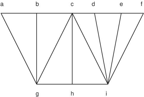
For any $p/q$, there are infinitely many edge paths in the Farey graph that begin at $1/0$ and end at $p/q$, but only finitely many that are minimal. A path is minimal if it never backtracks and if it never traverses two edges of the same triangle. The minimal paths for $K_{7/17}$ and their corresponding continued fractions are shown in the first two columns of Table 1. In general, only one of the minimal paths is even, that is, all the partial quotients are even. In Table 1, the first path is even. According to Hatcher and Thurston, each minimal path determines a boundary slope. The slope can be computed from the path $\gamma$ by the formula

where $\gamma_{even}$ is the even path and $m(\gamma)$ is the sum of the determinants of each edge of the path, excluding the first edge. Thus, the even path always gives a slope of zero. For any path $\gamma$, we call $m(\gamma)$ the unadjusted slope. The last two columns of Table 1 give the unadjusted slopes and the boundary slopes of $K_{7/17}$.

For any $p/q$, if $\gamma_{1}$ and $\gamma_{2}$ are two paths from $1/0$ to $p/q$, then we can move from one path to the other by a sequence of triangle moves. By a triangle move, we mean replacing two consecutive edges that lie in a single triangle with the third edge of the triangle, or vice-versa. If $\gamma_{1}$ is changed to $\gamma_{2}$ by a single triangle move, and furthermore, the triangle lies on the right of $\gamma_{1}$, then we call the move a right triangle move. Right triangle moves define a partial order on the set of paths: we say that $\gamma_{1}>\gamma_{2}$ if $\gamma_{1}$ can be changed to $\gamma_{2}$ by a sequence of right triangle moves. Furthermore, it is shown in [9] that right triangle moves strictly decrease the unadjusted slope of the path, thus, $\gamma_{1}>\gamma_{2}$ implies that $m(\gamma_{1})>m(\gamma_{2})$. The upper and lower minimal paths can now be defined as ones that are either maximal or minimal with respect to this partial order, respectively. These paths are well-defined because there is a unique minimal path with no triangles on its left and a unique minimal path with no triangles on its right. In Table 1, the first path is the upper path and the last path is the lower path.

The following lemma gives a lower bound on the number of distinct boundary slopes.

As the number $m$ of partial quotients grows, it becomes tedious to characterize all knots with $m$ partial quotients and exactly $k$ distinct boundary slopes. Therefore, in the following theorem, we only classify 2-bridge knots with up to four distinct boundary slopes. Furthermore, we provide the set of slopes for only one knot from each chiral pair. (Remember that switching from a knot to its mirror image will negate the set of boundary slopes.)

Proof. Suppose that $K_{p/q}$ has 4 or less distinct boundary slopes and strongly positive continued fraction expansion $p/q=0+[a_{1},a_{2},...,a_{m}]$. By Lemma 3.1, it follows that $m\leq 4$. We will examine only the case $m=3$ and leave the remaining cases, which are handled in a similar manner, to the interested reader.

Figure 3 shows all possible minimal paths for $p/q=[a_{1},a_{2},a_{3}]$ arranged according to the partial ordering on paths. Each of the five figures is made up of three main triangles which are subdivided into $a_{1}$, $a_{2}$, and $a_{3}$ smaller triangles, respectively, as we move from left to right. The five paths $\gamma_{\text{upper}}$, $\gamma_{1}$, $\gamma_{2}$, $\gamma_{3}$, and $\gamma_{\text{lower}}$ are depicted with heavy dark lines. Also listed is the unadjusted slope $m$ for each path under the path’s label.

Since $a_{1}>1$ and $a_{3}>1$ we have that $\gamma_{\text{upper}}$, $\gamma_{1}$, $\gamma_{2}$, and $\gamma_{\text{lower}}$ are minimal. If $\gamma_{3}$ is minimal and $a_{1}\neq a_{3}$, then we would have 5 distinct boundary slopes. Therefore, we have two cases to consider.

Assume $\gamma_{3}$ is not minimal, which requires $a_{2}=1$, and also that $a_{1}\neq a_{3}$. Thus, $p/q=0+[a_{1},1,a_{3}]$ and we have four distinct boundary slopes. In order to compute the (adjusted) slopes we need to determine the unique even path. Notice that

and so in order for $q$ to be odd we need at least one of $a_{1}$ or $a_{3}$ to be odd. This gives three sub-cases which are listed below.

These slopes appear in parts $4_{ii}$ and $4_{iii}$ of Theorem 3.2. The first two rows correspond to equivalent knots and only appear in one row of the theorem.

Next assume that $\gamma_{3}$ is not minimal and $a_{1}=a_{3}$. In this case, we have 3 distinct boundary slopes and

Here $q$ is odd if and only if $a_{1}$ is odd. In this case, the even path is $\gamma_{\text{lower}}$ and the boundary slopes are

where the second slope $-2a_{1}-2$ has multiplicity two, that is, it corresponds to two paths, $\gamma_{1}$ and $\gamma_{2}$. This data appears in part $3_{iii}$ of Theorem 3.2.

Finally, assume that $\gamma_{3}$ is minimal, which means $a_{2}>1$, and $a_{1}=a_{3}$. We now have four distinct boundary slopes and

In order for $q=a_{1}^{2}a_{2}+2a_{1}$ to be odd we must have that both $a_{1}$ and $a_{2}$ are odd. This implies that $\gamma_{\text{lower}}$ is the even path and we obtain the following boundary slopes:

Notice that the second boundary slope $-2a_{1}-2a_{2}$ has multiplicity two. This data appears in part $4_{i}$ of Theorem 3.2. The remaining cases follow by a similar analysis with $m=1$, $m=2$, or $m=4$. $\Box$

By working out the fractions $p/q$ for each case of Theorem 3.2 we obtain the following corollary which strengthens Theorem 3 of [14]. As in Theorem 3.2, we consider a knot and its mirror image to be equivalent.

In this section we briefly review the method of Ohtsuki, Riley, and Sakuma for constructing a pair of two bridge knots $K_{p^{\prime}/q^{\prime}}$ and $K_{p/q}$ with $K_{p^{\prime}/q^{\prime}}\geq K_{p/q}$. The reader is encouraged to consult [16] for a more detailed description. One begins with any 2-bridge knot (or link) $K_{p/q}$ given by the four-plat shown in Figure 4. The 4-string braid defining $K_{p/q}$ is denoted by $\beta$. There are three associated braids $\beta^{-1},\beta_{-}$, and $\beta^{-1}_{-}$ which are obtained by rotating $\beta$ 180 degrees around an axis perpendicular to the plane of the diagram, reflecting $\beta$ through a plane perpendicular to the plane of the diagram, and the composition of these two motions, respectively. In order to construct a 2-bridge knot $K_{p^{\prime}/q^{\prime}}$ that is greater than $K_{p/q}$ we consider a 4-plat with an odd number of “boxes” each containing either $\beta,\beta^{-1},\beta_{-}$, or $\beta^{-1}_{-}$. Starting from the left in Figure 4, the first box contains $\beta$ and every other box after that contains $\beta$ or $\beta_{-}$. The remaining boxes each contain $\beta^{-1}$ or $\beta^{-1}_{-}$. Also between each braid box in $K_{p^{\prime}/q^{\prime}}$ we may insert an even number of half-twists in the middle two strands of the 4-plat. Finally, a branched fold map $f$ is constructed from the complement of $K_{p^{\prime}/q^{\prime}}$ onto the complement of $K_{p/q}$ as follows. The complement of $K_{p^{\prime}/q^{\prime}}$ is cut along a collection of parallel 2-spheres into two 3-balls and a number of $S^{2}\times I$’s. The complement of $K_{p/q}$ is decomposed into two 3-balls and a single $S^{2}\times I$. A continuous mapping is then defined in a piecewise manner. First each 3-ball “upstairs” is mapped by the identity onto a corresponding 3-ball “downstairs.” Next, each $S^{2}\times I$ containing one braid box upstairs is mapped homeomorphically onto the $S^{2}\times I$ downstairs in a way that depends on the presence of $\beta,\beta^{-1},\beta_{-}$, or $\beta^{-1}_{-}$. Finally, the mapping is extended to the remaining $S^{2}\times I$’s upstairs onto the 3-balls downstairs using 2-fold branched mappings that depend on the combinations of $\beta,\beta^{-1},\beta_{-}$, or $\beta^{-1}_{-}$ in the adjacent components. From the way that $f$ is constructed, the two meridional generators associated with the bridges at either end of the 4-plat diagram upstairs are taken to the corresponding generators downstairs. Furthermore, the longitude upstairs is taken to a power of the longitude downstairs. Thus $f$ induces an epimorphism on fundamental groups which preserves peripheral structure.

Given a 2-bridge knot $K_{p/q}$, Ohtsuki, Riley and Sakuma determine which knots $K_{p^{\prime}/q^{\prime}}$ are produced by their construction. In particular, they show that $p^{\prime}/q^{\prime}$ gives such a knot if and only if it lies in the orbit of $p/q$ under the action of $\Gamma_{\infty}*\Gamma_{p/q}$, where $\Gamma_{r/s}$ is the infinite dihedral group generated by all reflections in edges of the Farey graph which end at $r/s$. Let $A_{1}$ and $A_{2}$ be generators of $\Gamma_{\infty}$ defined by reflection in the edges $<1/0,0/1>$ and $<1/0,1/1>$, respectively. For $p/q=[a_{1},a_{2},\dots,a_{m}]$ let $B_{1}$ and $B_{2}$ be generators of $\Gamma_{p/q}$ defined by reflection in the edges $<p/q,[a_{1},a_{2},\dots,a_{m-1}]>$ and $B_{2}=<p/q,[a_{1},a_{2},\dots,a_{m}-1]>$. Thus $p^{\prime}/q^{\prime}=W(p/q)$ where $W$ is a word in $A_{1},A_{2},B_{1}$ and $B_{2}$. Since $B_{1}$ and $B_{2}$ fix $p/q$, and $A_{1}$ and $A_{2}$ take $p/q$ to a fraction representing the same knot, we may assume that we begin by applying a nontrivial word in $A_{1}$ and $A_{2}$ and end by applying a nontrivial word in $B_{1}$ and $B_{2}$. Hence we may write $W$ as

where

Ohtsuki, Riley and Sakuma then show (Lemma 5.3 in [16]) that

where ${\bf a}$ is the vector ${\bf a}=(a_{1},a_{2},\dots,a_{m}),\ {\bf a}^{-1}$ means ${\bf a}$ written backwards, $\epsilon_{1}=1$, and $\epsilon_{i}=\prod_{j=1}^{i-1}-\eta_{j}$. The following lemma will prove helpful in simplifying continued fractions.

References

- [1] M Boileau, S Boyer, On character varieties, sets of discrete characters, and non-zero degree maps (2007)ArXiv:math.GT/0701384
- [2] M Boileau, S Boyer, R A, W S, Simon’s conjecture for 2-bridge knots (2009)ArXiv:math.GT/09032898
- [3] M Boileau, J H Rubinstein, S Wang, Finiteness of 3-manifolds associated with non-zero degree mappings (2005)ArXiv:math/0511541
- [4] G Burde, H Zieschang, Knots, volume 5 of de Gruyter Studies in Mathematics, Walter de Gruyter & Co., Berlin (2003)
- [5] D Cooper, M Culler, H Gillet, D D Long, P B Shalen, Plane curves associated to character varieties of -manifolds, Invent. Math. 118 (1994) 47–84
- [6] F González-Acuña, A Ramírez, Two-bridge knots with property Q, Quart. J. Math. 52 (2001) 447–454
- [7] A Hatcher, W Thurston, Incompressible surfaces in -bridge knot complements, Invent. Math. 79 (1985) 225–246
- [8] J Hoste, P D Shanahan, A formula for the A-polynomial of twist knots, J. Knot Theory Ramifications 13 (2004) 193–209
- [9] J Hoste, P D Shanahan, Boundary slopes of 2-bridge links determine the crossing number, Kobe J. Math. 24 (2007) 21–39
- [10] K Ichihara, S Mizushima, Crossing number and diameter of boundary slope set of Montesinos knot, Comm. Anal. Geom. 16 (2008) 565–589
- [11] D Johnson, C Livingston, Peripherally specified homomorphs of knot groups, Trans. Amer. Math. Soc. 311 (1989) 135–146
- [12] P B Kronheimer, T S Mrowka, Witten’s conjecture and Property P, Geom. Topol. 8 (2004) 295–310
- [13] M Macasieb, K Petersen, R Van Luijk, On character varieties of two-bridge knot groups ArXiv:math.GT/09022195
- [14] T Mattman, G Maybrun, K Robinson, 2-Bridge knot boundary slopes: diameter and genus, Osaka J. Math. 45 (2008) 471–489
- [15] T Ohtsuki, Ideal points and incompressible surfaces in two-bridge knot complements, J. Math. Soc. Japan 46 (1994) 51–87
- [16] T Ohtsuki, R Riley, M Sakuma, Epimorphisms between 2-bridge link groups, from: “The Zieschang Gedenschrift, Geom. Top. Monographs”, volume 14, Geom. Top. Publ., Coventry (2008) 417–450
- [17] R Riley, Nonabelian representations of -bridge knot groups, Quart. J. Math. Oxford Ser. (2) 35 (1984) 191–208
- [18] D S Silver, W Whitten, Knot group epimorphisms, J. Knot Theory Ramifications 15 (2006) 153–166