Supersolvable lattices of $J$ -classes

Mahir Bilen Can

Date: October 21, 2009

Abstract.

The purpose of this article is to investigate the combinatorial properties of the cross section lattice of a $J$ -irreducible monoid associated with a semisimple algebraic group of one of the types $A_{n}$ , $B_{n}$ , or $C_{n}$ . Our main tool is a theorem of Putcha and Renner which identifies the cross section lattice in the Boolean lattice of subsets of the nodes of a Dynkin diagram. We determine the join irreducibles of the cross section lattice. Exploiting this we find characterizations of the relatively complemented intervals. By a result of Putcha, this determines the Möbius function for $\Lambda$ . We show that an interval of the cross section lattice is Boolean if and only if it is relatively complemented if and only if it is atomic. We characterize distributive cross section lattices, showing that they are products of chains. We determine which cross section lattices are supersolvable, and furthermore, we compute the characteristic polynomials of these supersolvable cross section lattices.

1. Introduction

Let $K$ be an algebraically closed field, and let $G_{0}$ be a semisimple linear algebraic group over $K$ . Let $\rho:G_{0}\rightarrow GL(V)$ be an irreducible representation of $G_{0}$ , and let $G=K^{*}\cdot\rho(G_{0})$ be the image of $G_{0}$ under $\rho$ , adjoined by the scalar matrices. The $J-irreducible\ monoid$ $M$ associated with the pair $(G_{0},\rho)$ is the Zariski closure of the group $G$ in $End(V)$ (see [16]).

The group $G\times G$ acts on the monoid $M$ by $(g,h)\cdot x=gxh^{-1}$ , $x\in M,\ (g,h)\in G\times G$ . Let $J_{x}=GxG$ denote an orbit for some $x\in M$ . There is a natural partial ordering on the set $\{J_{x}:\ x\in M\}$ of orbits:

(1.1)

J_{e}\leq J_{f}\iff J_{e}\subseteq\overline{J_{f}},\ e,f\in M.

Here $\overline{J_{f}}$ denotes the Zariski closure of $J_{f}$ in $M$ .

In this manuscript we are concerned with the combinatorics of the set $\{J_{x}:\ x\in M\}$ of orbits. The above construction hints just a special case of a much more general theory of algebraic monoids which has been developed during the past 30 years largely by M.S. Putcha and L.E. Renner. The reader can find more about algebraic monoids in the books [12] and [17].

In [11], Putcha shows that there exists a finite cross section lattice of idempotents, denoted by $\Lambda$ , for the set of $G\times G$ -orbits. More precisely, there exists a finite set $\Lambda=\{e\in M:\ e^{2}=e\}$ of idempotents such that a) $\bigcup\{J_{e}:\ e\in\Lambda\}=\bigcup\{J_{x}:\ x\in M\}$ , b) if $x\in M$ , $|J_{x}\cap\Lambda|=1$ , c) $\Lambda$ is a graded lattice with respect to the partial ordering

(1.2)

J_{e}\leq J_{f}\iff J_{e}\subseteq\overline{J_{f}}\iff e=ef=fe,

with the rank function given by $rk(e)=\dim GeG$ . It turns out (see Chapter 6, [12]) that one can recover basic subgroups of the group $G$ from $\Lambda$ : the centralizer of $\Lambda$ in $G$ is a maximal torus

T=C_{G}(\Lambda)=\{g\in G:\ ge=eg,\ e\in\Lambda\},

and the right centralizer

B=C_{G}^{r}(\Lambda)=\{g\in G:\ ge=ege\ \text{for\ all}\ e\in\Lambda\}

of $\Lambda$ in $G$ is a Borel subgroup containing the maximal torus $T$ .

A remarkable theorem of Putcha and Renner identifies $\Lambda$ by a subposet of the Boolean lattice of all subsets of a set $\Delta$ of simple roots for $G$ . Before we state the Theorem, we explain briefly the terminology about simple roots and Coxeter diagrams (disjoint unions of Dynkin diagrams). The details can be found in [7].

Recall that simple algebraic groups are classified according to the discrete data of the “Dynkin diagrams.” There are four infinite families of simple groups, denoted by $A_{n},B_{n},C_{n},D_{n}$ , and five exceptional groups, denoted by $E_{6},E_{7},E_{8},F_{4},G_{2}$ . For each group in this list the Dynkin diagram is a connected “graph” as shown in the Figure 1.1. Let $T$ be a maximal torus in the simple group $G_{0}$ , and let $X(T)=\text{Hom}(T,K^{*})$ be the group of group homomorphisms from $T$ into $K^{*}$ . The nodes of a Dynkin diagram correspond to some special vectors, called simple roots, in the vector space $V=X(T)\otimes{\mathbb{Q}}$ . The set of simple roots is denoted by $\Delta$ . Each simple root $\alpha\in\Delta$ gives a reflection (with respect to the hyperplane perpendicular to $\alpha$ ) on $V$ , which is denoted by $\sigma_{\alpha}$ . The group generated by these involutions is called the standard reflection representation of the Weyl group of $G$ relative to $T$ . Here, a Weyl group¹¹ 1 More generally, for an algebraic group $G$ a Weyl group is defined to be the quotient group $W=N_{G}(T)/Z_{G}(T)$ , where $Z_{G}(T)=\{g\in G:\ gt=tg,\ \text{for all}\ t\in T\}$ is the centralizer of $T$ in $G$ . is defined to be the quotient of the normalizer $N_{G_{0}}(T)=\{g\in G:\ gT=Tg\}$ by $T$ .

When the group is not simple, one still has a diagram (as well as $\Delta$ ), called the Coxeter diagram, which is a disjoint union of the Dynkin diagrams of the simple components. A subset $Y\subseteq\Delta$ is called connected if it is a connected subset of the underlying graph of the Coxeter diagram.

Figure 1.1. Dynkin diagrams of the simple groups.

We turn back to the monoids. If $M$ is a $J-$ irreducible monoid, then $\Lambda$ has a unique minimal nonzero element, denoted by $e_{0}$ (Lemma 7.8, [17]).

Theorem 1.3.

(Putcha-Renner, [10]) Let $M$ be a $J$ -irreducible monoid with a cross section lattice $\Lambda$ . Let $T=C_{G}(\Lambda)$ , $B=C_{G}^{r}(\Lambda)$ . Let $\Delta$ be the set of simple roots of $T$ relative to $B$ . Let $2^{\Delta}$ be the Boolean lattice of all subsets of $\Delta$ . Define

\phi:\Lambda\longrightarrow 2^{\Delta}

\phi(e)=\{\alpha\in\Delta|\ \sigma_{\alpha}e=e\sigma_{\alpha}\neq e\}.

Here, $\sigma_{\alpha}$ is the simple reflection associated with the root $\alpha$ . Then

(i)

$\phi$ is injective and order preserving.
(ii)

$I\in 2^{\Delta}$ is in the image of $\phi$ iff no connected component of $I$ (in the Coxeter graph of $\Delta$ ) lies entirely in $J_{0}=\{\alpha\in\Delta|\ \sigma_{\alpha}e_{0}=e_{0}\sigma_{\alpha}\}$ where $e_{0}\in\Lambda-\{0\}$ is the minimal element.

The above theorem, which we exploit is the bridge between a cross section lattice and the combinatorics of finite sets. Now we can state our main results and give a brief summary of the article. In the next two sections we setup the notation and give the necessary background.

The Möbius function of a poset $P$ is the unique function $\mu:P\times P\rightarrow{\mathbb{N}}$ satisfying

(1)

$\mu(x,x)=1$ for every $x\in P$ ,
(2)

$\mu(x,y)=0$ whenever $x\nleq y$ ,
(3)

$\mu(x,y)=-\sum_{x\leq z<y}\mu(x,z)$ for all $x<y$ in $P$ .

It is well known that the set of all chains of a poset is a simplicial complex and the Möbius function is the reduced Euler characteristic of the associated topological space (see [24]). The Möbius function of a cross section lattice is computed by Putcha:

Theorem 1.4.

(Putcha, [14]) Let $\Lambda$ be a cross section lattice of an algebraic monoid. Let $e\leq f$ be in $\Lambda$ . Then,

(1.5)

\mu(e,f)=\begin{cases}(-1)^{rk(f)-rk(e)}&\text{if}\ [e,f]\ \text{is relatively complemented,}\\ 0&otherwise.\end{cases}

Here relatively complemented means that for every interval $[x,y]\subseteq L$ , and for every $z\in[x,y]$ , there exists $z^{\prime}\in[x,y]$ such that $z\vee z^{\prime}=y$ and $z\wedge z^{\prime}=x$ .

In Section 3 we describe a method for deciding when an interval $[e,f]$ in $\Lambda$ is relatively complemented. We use the notation $\Lambda^{*}$ to denote $\Lambda-\{0\}$ .

Theorem 1.6.

We use the notation of the Theorem 1.3. In particular, let $J_{0}=\{\alpha\in\Delta|\ \sigma_{\alpha}e_{0}=e_{0}\sigma_{\alpha}\}$ where $e_{0}\in\Lambda^{*}$ is the minimal element. Then, for $e\leq f$ in $\Lambda$ , the interval $[e,f]$ is relatively complemented if and only if there does not exist $\alpha\in J_{0}$ such that $\alpha\in\phi(f)-\phi(e)$ and $\sigma_{\alpha}\sigma_{\beta}=\sigma_{\beta}\sigma_{\alpha}$ for every $\beta\in\phi(e)$ .

A graded lattice $L$ is called (upper) semimodular if the following inequality

(1.7)

rk(x)+rk(y)\geq rk(x\wedge y)+rk(x\vee y)

holds for all $x,y\in L$ . It is known that $\Lambda$ of a $J-$ irreducible monoid is upper semimodular. The lattice $L$ is called atomic if every element is a join of atoms (elements covering $\hat{0}$ ).

Recall that (see [24]) a semimodular lattice is relatively complemented if and only if it is atomic. As a corollary, we also prove that

Corollary 1.8.

An interval of $\Lambda^{*}$ is relatively complemented if and only if it is atomic if and only if it is isomorphic to a Boolean lattice.

Recall that a lattice $Z$ is called distributive if for every $a,b$ and $c$ from $Z$ , $a\wedge(b\vee c)=(a\wedge b)\vee(a\wedge c)$ hold. It is observed in [10] that $\Lambda$ is a distributive lattice whenever $\Delta-J_{0}$ is a connected subset of the Coxeter graph of $\Delta$ , where $\Delta$ and $J_{0}$ are as before. In Section 4, we prove:

Theorem 1.9.

Let $\Lambda$ be the cross section lattice of a $J-$ irreducible monoid of the pair $(G_{0},\rho)$ , where $G_{0}$ is a simple algebraic group of one of the types $A_{n},B_{n}$ or $C_{n}$ . Let $J_{0}$ be as in the Theorem 1.3, and let $\Delta$ be the set of simple roots. Suppose $|J_{0}|>1$ . Then, the followings are equivalent.

(1)

$\Lambda^{*}$ is a distributive lattice,
(2)

$\Lambda^{*}$ is isomorphic to a product of chains,
(3)

$\Lambda^{*}$ is isomorphic to a sublattice of a Boolean lattice.

A particularly interesting class of distributive cross section lattices are studied by Renner in [18].

Let $M$ be a $J-$ irreducible monoid, and let $\Lambda$ be the cross section lattice. Let $T=C_{G}(\Lambda)$ be the maximal torus associated with $\Lambda$ , and let $W=N_{G}(T)/T$ be the Weyl group as before. Then, $W$ acts on $V=X(T)\otimes{\mathbb{Q}}$ via its reflection representation, where $X(T)=\text{Hom}(T,K^{*})$ . Let $\mu\in V$ be a vector which is in general position with respect to lines determined by the simple roots $\Delta\subseteq V$ . Let $\mathcal{P}_{\mu}=Conv(W\cdot\mu)\subseteq V$ be the polytope obtained by taking the convex hull of the set of points $\{w\cdot\mu:\ w\in W$ } in $V$ . Let $P=P_{\mu}$ be the (projective) toric variety associated with this polytope.

Assume, temporarily, that $K={\mathbb{C}}$ . Let $O$ be a variety over $K$ of dimension $n$ . The variety $O$ is called rationally smooth at $x\in O$ , if for every point $y\in U\subseteq O$ in a neighborhood of $x\neq y$ the cohomology groups $H_{y}^{i}(O)=H^{i}(O;O-\{y\},{\mathbb{Q}})$ vanish except at the top dimension, which is 1 dimensional. In other words,

H^{i}_{y}(O)=0\ \text{for}\ i\neq 2n,\ \text{and}

H^{2n}_{y}(O)={\mathbb{Q}}.

In [18], Renner calls a subset $J\subset S=S(\Delta)=\{\sigma_{\alpha}:\ \alpha\in\Delta\}$ of the simple generators of $W$ by combinatorially smooth, if the toric variety $O=P$ associated with the polytope $\mathcal{P}_{\mu}$ is rationally smooth at every point. In his paper, Renner lists all combinatorially smooth subsets for a Weyl group. Looking at his table one sees that ²² 2 for the sake of space we mention type $A_{n}$ , $n\geq 2$ only. the subset $J$ is combinatorially smooth if $J\subseteq\{\alpha_{1},...,\alpha_{n}\}$ is equal to one of the followings:

(1)

$J_{0}=\emptyset$ ,
(2)

$J_{0}=\{\alpha_{1},...,\alpha_{i}\}$ where $1\leq i<n$ ,
(3)

$J_{0}=\{\alpha_{j},...,\alpha_{n}\}$ where $1<j\leq n$ ,
(4)

$J_{0}=\{\alpha_{1},...,\alpha_{i},\alpha_{j},...,\alpha_{n}\}$ where $1\leq i,j\leq n$ and $j-i\geq 3$ .

In other words in type $A_{n}$ $P$ is a rationally smooth toric variety, then $\Lambda^{*}$ is distributive. However, the converse need not to be true: In Figure 1.2 we have an example of a cross section lattice such that the associated toric variety is not rationally smooth.

Figure 1.2. Combinatorially non-smooth but distributive

\Lambda^{*}

This motivates us to understand the structure of a distributive $\Lambda^{*}$ more precisely. Thus, we make the following conjecture:

Conjecture 1.10.

Let $\Lambda$ be a distributive cross section lattice of the $J$ -irreducible monoid of the pair $(G_{0},\rho)$ , where $G_{0}$ is a simple algebraic group of one of the types $A_{n-1},B_{n-1}$ or $C_{n-1}$ . Let $J_{0}$ and $\Delta=\{\alpha_{1},...,\alpha_{n-1}\}$ be the set of simple roots as in Theorem above. Suppose that $J_{0}$ has connected components $J_{0}^{(1)}=\{\alpha_{1},\alpha_{2},...,\alpha_{k}\}$ and $J_{0}^{(2)}=\{\alpha_{l},\alpha_{l+1},...,\alpha_{n-1}\}$ (with possibility that $J_{0}^{(1)}=\emptyset\ \text{or that}\ J_{0}^{(2)}=\emptyset$ ). Then $\Lambda^{*}$ is isomorphic to the product of the chains:

C_{k+2}\times C_{n-l+2}\times C_{2}^{l-k-3}=C_{k+2}\times C_{n-l+2}\times C_{2}\times\cdots\times C_{2}.

Suppose that $L$ is a finite lattice, and let $\varGamma$ be a maximal chain such that for every chain $\varGamma^{\prime}$ of $L$ , the sublattice generated by $\varGamma$ and $\varGamma^{\prime}$ is distributive. Such a lattice $L$ is called supersolvable, and the maximal chain $\varGamma$ is called an $\mathcal{M}$ -chain. This notion about lattices, introduced and used by Stanley [22] is a direct generalization of the supersolvability of a group (where there is a series of normal subgroups with all the factors are cyclic groups). In Section 5, we determine the supersolvable cross section lattices with respect to $J_{0}$ . More precisely, we prove that

Theorem 1.11.

Let $\Delta=\{\alpha_{1},...,\alpha_{n}\}$ be the set of simple roots and $J_{0}$ be as before. Then, the cross section lattice $\Lambda$ is supersolvable if and only if a connected component of $J_{0}$ is either a singleton $\{\alpha_{i}\}$ for some $\alpha_{i}\in\Delta$ , or is a subset $\widetilde{J_{0}}\subseteq\Delta$ whose induced subgraph in the Dynkin diagram is connected and contains an end node of $\Delta$ .

Here, a simple root $\alpha\in\Delta$ is called an end-node if there exists a unique $\alpha^{\prime}$ in $\Delta$ such that $\sigma_{\alpha}\sigma_{\alpha^{\prime}}\neq\sigma_{\alpha^{\prime}}\sigma_{\alpha}$ where $\sigma_{\alpha^{\prime}}$ is the simple reflection associated with the root $\alpha^{\prime}$ .

We prove this theorem by exhibiting an $\mathcal{M}$ -chain $\varGamma$ as in the definition of the supersolvability.

The characteristic polynomial of a graded poset $P$ with $\hat{0}$ and $\hat{1}$ is

(1.12)

p(x,P)=\sum_{x\in P}\mu(\hat{0},x)x^{rk(\hat{1})-rk(x)}.

Here $rk:P\rightarrow{\mathbb{N}}$ is the rank function, and $\mu$ is the Möbius function on $P$ .

Theorem 1.13.

(Stanley, [22]) Let $L$ be a semimodular supersolvable lattice. Let $\hat{0}=x_{0}<x_{1}<\cdots<x_{n}=\hat{1}$ be an $\mathcal{M}$ -chain. Then,

(1.14)

p(x,L)=(x-a_{1})(x-a_{2})\cdots(x-a_{n}),

where $a_{i}$ is the number of atoms $u\in L$ such that $u\leq x_{i}$ and $u\nleq x_{i-1}$ .

In Section 6, using the above theorem of Stanley we prove

Theorem 1.15.

Let $\Lambda^{*}$ be a supersolvable cross section lattice of a $J-$ irreducible monoid of the pair $(G_{0},\rho)$ , where $G_{0}$ is a simple algebraic group of one of the types $A_{n},B_{n}$ or $C_{n}$ . Let $J_{0}\subseteq\Delta$ be as before, and let $n=|\Delta|$ . Then the characteristic polynomial of $\Lambda^{*}$ is

(1.16)

p(x,\Lambda^{*})=x^{|J_{0}|}(x-1)^{n-|J_{0}|}.

Based on computer experiments, we conjecture that

Conjecture 1.17.

Let $\Lambda^{*}$ be the cross section lattice of a ( $J-$ irreducible) monoid $M$ . Then

(1.18)

p(x,\Lambda^{*})=x^{|J_{0}|}(x-1)^{n-|J_{0}|}.

Even though we state our theorems only for the $J$ -irreducible monoids of the types $A_{n}$ , $B_{n}$ and $C_{n}$ the reader will not have difficulty in proving similar results for the other types.

2. Preliminaries

2.1. Poset terminology

The unexplained terminology about posets and (quasi) symmetric functions can be found in the books [24] and [25]. We assume that all posets and lattices are finite, and furthermore have a minimal element, denoted by $\hat{0}$ , as well as a maximal element which is denoted by $\hat{1}$ .

Let $\Delta$ be a finite set (which is going to stand for the set of simple roots). We use the notation $2^{\Delta}$ to denote the Boolean lattice of all subsets of $\Delta$ with the partial order of inclusion.

For any integer $m>0$ we denote $\{1,...,m\}$ by $[m]$ . An increasing sequence of numbers $m_{1}<m_{2}<\cdots<m_{k}$ is denoted by $\{m_{1},...,m_{k}\}_{<}$ .

A composition $\gamma$ of a positive integer $m$ is an ordered sum of positive integers whose sum is $m$ . The set of all compositions of $m$ is denoted by $Comp(m)$ . A partition $\lambda$ of a positive integer $m$ is an unordered sum of positive integers whose sum is $m$ . There is a $1-1$ correspondence between subsets of $\{1,...,m-1\}$ and compositions of $m$ which is defined by sending $\gamma=\gamma_{1}+\cdots+\gamma_{k}$ to $S_{\gamma}=\{\gamma_{1},\gamma_{1}+\gamma_{2},...,\gamma_{1}+\cdots\gamma_{k-1}\}$ . For a composition $\gamma$ of $m$ , $\lambda=\lambda(\gamma)$ denotes the partition of $m$ obtained by rewriting the entries of $\gamma$ in a decreasing order.

Let $P$ be a graded poset of rank $n$ with $\hat{0}$ and $\hat{1}$ . Equivalently, $P$ has the smallest and the largest elements and every maximal chain in $P$ is of the same length $n$ . Let $rk:P\rightarrow{\mathbb{N}}$ be the rank function, so that $rk(x)\in{\mathbb{N}},\ x\in P$ is the length of the maximal chain from $\hat{0}$ to $x$ . If $x\leq y$ in $P$ , then the length of the interval $[x,y]=\{z\in P:\ x\leq z\leq y\}$ is defined to be

(2.1)

rk(x,y)=rk(y)-rk(x).

A graded poset $P$ of rank $n$ is called locally rank symmetric if every interval of $P$ is rank-symmetric, i.e., has the same number of elements of rank $i$ as of corank $i$ for all $i$ . Here corank of an element $x\in P$ means $n-rk(x)$ .

The set of all chains in an interval $I$ (resp. in $P=[\hat{0},\hat{1}]$ ) of $P$ is denoted by $\mathcal{C}(I)$ (resp. by $\mathcal{C}$ ). Similarly, the set of all max chains in $I$ (resp. in $P=[\hat{0},\hat{1}]$ ) of $P$ is denoted by $\mathcal{C}_{max}(I)$ (resp. by $\mathcal{C}_{max}$ ).

The rank set $rk(\tau)$ of a chain $\tau=(t_{1}<\ldots<t_{i})\in\mathcal{C}$ is defined to be

(2.2)

rk(\tau)=\{m_{i}:\ m_{i}=rk(t_{i})\}_{<}.

Let $n$ be the rank of $P$ , and let $I,J\subseteq\{1,\ldots,n-1\}$ . Define

(2.3)		$\displaystyle\alpha_{P}(I)$	$\displaystyle=$	$\displaystyle\|\{\tau:\ rk(\tau)=I\}\|,$
(2.4)		$\displaystyle\beta_{P}(J)$	$\displaystyle=$	$\displaystyle\sum_{I\subseteq J}(-1)^{\|J-I\|}\alpha_{P}(I).$

The function $\alpha_{P}$ (from the set of all subsets of $[rk(P)]$ into ${\mathbb{N}}$ ) is sometimes called the flag $f$ -vector of $P$ .

The formal power series

(2.5)

F_{P}(x)=\sum_{\hat{0}=t_{0}\leq t_{1}\leq\cdots\leq t_{k-1}<t_{k}=\hat{1}}x_{1}^{rk(t_{0},t_{1})}x_{2}^{rk(t_{1},t_{2})}\cdots x_{k}^{rk(t_{k-1},t_{k})},

where the sum is over all multichains from $\hat{0}$ to $\hat{1}$ such that $\hat{1}$ occurs exactly once is introduced by Ehrenborg in [4]. In [23], Stanley shows that

F_{P}=\sum_{I\subseteq[n-1]}\beta_{P}(I)F_{I,n},

where

(2.6)

F_{I,n}=\sum_{j_{1}\leq\cdots\leq j_{n}\atop i\in I\Rightarrow j_{i}<j_{i+1}}x_{j_{1}}\cdots x_{j_{n}},

are the fundamental quasi-symmetric functions. A poset $P$ is called flag-symmetric if the function $F_{P}$ is a symmetric function.

Let $L$ be a lattice (hence joins “ $\vee$ ” and the meets “ $\wedge$ ” exist). $L$ is called relatively complemented, if for every interval $[x,y]\subseteq L$ , and for every $z\in[x,y]$ , there exists $z^{\prime}\in[x,y]$ such that $z\vee z^{\prime}=y$ and $z\wedge z^{\prime}=x$ . A lattice $L$ is called atomic if every element of $L$ is the join of atoms (elements covering $\hat{0}$ ) of $L$ .

A graded lattice $L$ is called (upper) semimodular if the following inequality

(2.7)

rk(x)+rk(y)\geq rk(x\wedge y)+rk(x\vee y)

holds for all $x,y\in L$ . Equivalently (Birkhoff’s characteriztion): if $x$ covers $x\wedge y$ , then $x\vee y$ covers $y$ . In an (upper) semimodular lattice $L$ being relatively complemented is equivalent to being atomic (see Proposition 3.3.3., [24]).

A graded lattice $L$ is called modular if the inequality in (2.7) is equality for all $x,y\in L$ . A lattice $L$ is called distributive if for all $x,y,z\in L$ the following holds

(2.8)

x\wedge(y\vee z)=(x\wedge y)\vee(x\wedge z).

It is easy to show that a distributive lattice is modular.

A pair $(a,b)$ of elements of $L$ is called a modular pair, if the following holds

(2.9)

c\leq b\Rightarrow c\vee(a\wedge b)=(c\vee a)\wedge b.

It is convenient to denote a modular pair by $a\mathcal{M}b$ . An element $b\in L$ is called right modular if $x\mathcal{M}b$ for every $x\in L$ . Similarly, an element $a\in L$ is called left modular if $a\mathcal{M}x$ for every $x\in L$ . It is easy to see that a lattice is modular if and only if every ordered pair of elements of $L$ is modular.

2.2. Reductive groups and monoids

The purpose of this section is to introduce the notation of the reductive monoids. We focus mainly on the orbit structure of these monoids. For more details the reader should consult [17] or [12]. For an introduction, with many explicit examples, we suggest the survey by Solomon [21]. For more background on the theory of algebraic groups, we suggest Humphrey’s book [7].

Our basic list of notation for groups is as follows.

(2.10)	$\displaystyle G$	$\displaystyle=\text{reductive group,}$
(2.11)	$\displaystyle B$	$\displaystyle=\text{Borel subgroup,}$
(2.12)	$\displaystyle T$	$\displaystyle=\text{maximal torus contained in $B$,}$
(2.13)	$\displaystyle W$	$\displaystyle=N_{G}(T)/T=\text{Weyl group of}\ (G,T),$

An algebraic monoid is a variety $M$ together with

(1)

an associative morphism

$m:M\times M\rightarrow M$
(2)

a unity $1\in M$ with $m(1,x)=m(x,1)=x$ for all $x\in M$ .

The set $G=G(M)$ of invertible elements of $M$ is an algebraic group. If $G$ is a reductive group and $M$ is irreducible $M$ is called a reductive monoid. It turns out [20] that the reductive monoids are exactly the affine, two-sided embeddings of connected reductive groups.

Many interesting examples of (reductive) monoids are obtained as the Zariski closures $\overline{K\cdot G}\subseteq End(V)$ of (representations of) reductive groups in a space of endomorphisms on a linear space $V$ .

In a reductive monoid, the data of the Weyl group $W$ of the reductive group $G$ and the set $E(\overline{T})$ of idempotents of the embedding $\overline{T}\hookrightarrow M$ combine to become a finite inverse semigroup $R=\overline{N_{G}(T)}/T\cong W\cdot E(\overline{T})$ with unit group $W$ and idempotent set $E(R)=E(\overline{T})$ . The inverse semigroup $R$ , controls the Bruhat decomposition for the algebraic monoid $M$ . Recall that the Bruhat-Chevalley order on the Weyl group $W$ is defined by

x\leq y\ \mbox{iff}\ BxB\subseteq\overline{ByB},

where $B$ is a Borel subgroup of $G$ . Similarly, on the Renner monoid $R$ of a reductive monoid $M$ , the Bruhat-Chevalley order is defined by

(2.14)

\sigma\leq\tau\ \mbox{iff}\ B\sigma B\subseteq\overline{B\tau B}.

One observes that the induced poset structure on $W$ , which is induced from $R$ is the same as the original Bruhat poset structure on $W$ .

Let $T$ be a maximal torus and $E(\overline{T})$ be the set of idempotent elements in the (Zariski) closure of $T\subseteq G$ in the monoid $M$ . Similarly, let us denote by $E(M)$ the set of idempotents in the monoid $M$ . Plainly we have $E(\overline{T})\subseteq E(M)$ . There is a canonical partial order $\leq$ on $E(M)$ (hence on $E(\overline{T})$ ) defined by

(2.15)

e\leq f\ \Leftrightarrow\ ef=e=fe.

Notice that $E(\overline{T})$ is invariant under the conjugation action of the Weyl group $W$ . We call a subset $\Lambda\subseteq E(\overline{T})$ as a cross-section lattice if $\Lambda$ is a set of representatives for the $W$ -orbits on $E(\overline{T})$ and the bijection $\Lambda\rightarrow G\backslash M/G$ defined by $e\mapsto GeG$ is order preserving. It turns out that we can write $\Lambda=\Lambda(B)=\{e\in E(\overline{T}):\ Be=eBe\}$ for some unique Borel subgroup $B$ containing $T$ . The partial order given by (2.15) on $E(\overline{T})$ (hence on $\Lambda$ ) agrees with the Bruhat-Chevalley order (2.14) on the Renner monoid.

The decomposition $M=\bigsqcup_{e\in\Lambda}GeG$ , of a reductive monoid $M$ into its $G\times G$ orbits, has a counterpart on the Renner monoid $R$ of $M$ . Namely, the finite monoid $R$ can be written as a disjoint union

(2.16)

R=\bigsqcup_{e\in\Lambda}WeW

of $W\times W$ orbits, parametrized by the cross section lattice.

It is shown by Putcha [13] that each orbit $WeW$ , for $e\in\Lambda$ , is a lexicographically shellable poset. Notice, as a special case, that if $e\in\Lambda$ is the identity element of $G$ , then the orbit $WeW$ is the Weyl group $W$ , and the lexicographically shellability of the Coxeter groups is well known [2], [9]. The author shows in [3] that the Renner monoid (so called rook monoid) of the monoid of $n\times n$ matrices is lexicographically shellable. The question of shellability of a Renner monoid in general is still an open problem.

It is known that $E(\overline{T})$ is a relatively complemented lattice, anti-isomorphic to a face lattice of a convex polytope. Let $\Lambda$ be a cross section lattice in $E(\overline{T})$ . The Weyl group of $T$ (relative to $B=C_{G}^{r}(\Lambda)$ ) acts on $E(\overline{T})$ , and furthermore

(2.17)

E(\overline{T})=\bigsqcup_{w\in W}w\Lambda w^{-1}.

It is shown by Putcha [Corollary 8.12, [12]] that if $\emptyset\neq\varGamma\subseteq E(\overline{T})$ is such that $(\varGamma,\leq)$ is a relatively complemented lattice with all maximal chains having length equal to $\dim T$ , then $\varGamma=E(\overline{T})$ . Therefore, the cross section lattice $\Lambda\subseteq E(\overline{T})$ is relatively complemented if and only if $\Lambda=E(\overline{T})$ , and this is possible if and only if $W$ is trivial.

A reductive monoid with $0$ is called $J-$ irreducible if there exists a unique minimal, nonzero $G\times G$ orbit (= a $J$ -class). This explains the terminology. Notice that this is equivalent to the fact that $\Lambda$ has a unique minimal nonzero element $e_{0}\in\Lambda$ . One of the many reasons to be interested in $J-$ irreducible monoids is a theorem of Renner [16], which shows that a monoid $M$ is $J-$ irreducible if and only if there exists a rational representation $\rho:M\rightarrow End(K^{n})$ such that $\rho$ is a finite morphism, and $K^{n}$ is an irreducible module for $M$ .

3. The cross section of a $J-$ irreducible monoid

Let $\alpha\in\Delta$ be a simple root. We denote by $\sigma_{\alpha}$ the simple reflection corresponding to $\alpha$ . Let $\Lambda^{*}=\Lambda-\{0\}$ .

The following theorem of Putcha and Renner is one of the crucial steps in determining the structure of the cross section lattice of a $J-$ irreducible monoid.

Theorem 3.1.

(Putcha and Renner, Theorem 4.13, [10]) We use the notation of the Theorem 1.3. Let $e\in\Lambda^{*}$ . Then there is a one to one correspondence between $\{\alpha\in\Delta:\ \sigma_{\alpha}e\neq e\sigma_{\alpha}\}$ in $\Delta$ and $\{f\in\Lambda:\ f\ \text{covers}\ e\}$ . Furthermore, $\alpha$ corresponds to the unique $f=f_{\alpha}$ with $\phi(f)=\phi(e)\cup\{\alpha\}$ .

By Theorem 1.3, we see that $\phi(e\wedge f)$ is the largest subset $U$ of $\phi(e)\cap\phi(f)$ such that there exists an idempotent $h\in\Lambda$ with $U=\phi(h)$ . Therefore, the following corollary of Theorem 3.1 (and Theorem 1.3) is straightforward.

Corollary 3.2.

Let $e,f\in\Lambda$ , and let $U=\phi(e),\ V=\phi(f)$ . Then,

(1)

$\alpha\in\phi(e\wedge f)$ if and only if $\alpha\in U\cap V$ , and $J_{0}$ does not contain the connected component in $U\cap V$ of $\alpha$ .
(2)

If $V\cap J_{0}=\emptyset$ , then $\phi(e\wedge f)=U\cap V$ .
(3)

If $V\cap J_{0}=\emptyset$ , then for any subset $Y\subseteq V$ there exists $h\in\Lambda$ such that $h\leq f$ and $Y=\phi(h)$ .

The following, which was already known to the experts (see Remark 3.6, [13]) is also a straightforward corollary of the above considerations.

Corollary 3.3.

Let $e_{0}\in\Lambda$ be the minimal nonzero idempotent. Then, $\Lambda$ is an (upper) semimodular lattice. Furthermore, the value of the rank function $e\mapsto\dim(eT)$ on $\Lambda$ is equal to $|\phi(e)|=|\{\alpha\in\Delta:\ \sigma_{\alpha}e=e\sigma_{\alpha}\neq e\}|$ .

Proof.

By Theorems 3.1 and 1.3, $\phi(e\vee f)=\phi(e)\cup\phi(f)$ . If $e$ covers $e\vee f$ , then there exists a unique $\beta\in\phi(e)-\phi(f)$ such that $\phi(e)=\phi(e\wedge f)\cup\{\beta\}$ . Then, $\phi(e\vee f)=\phi(e)\cup\phi(f)=\phi(f)\cup\{\beta\}$ . In other words, $e\vee f$ covers $f$ . This proves the semimodularity. The second assertion is straightforward from Theorems 3.1 and 1.3, also. ∎

The set of join irreducibles of $\Lambda^{*}$ is found as follows.

Definition 3.4.

Let $J\subseteq\Delta$ be a subset of the nodes of the Dynkin diagram. A subset $A=\{\alpha_{1},...,\alpha_{k}\}$ of $J$ is called a connected subset if the subgraph of the Dynkin diagram induced by $A$ is connected. Therefore, if $|A|>1$ , then for each $\alpha_{i}\in A$ there exists $\alpha_{j}\neq\alpha_{i}$ in $A$ such that $\sigma_{\alpha_{i}}\sigma_{\alpha_{j}}\neq\sigma_{\alpha_{j}}\sigma_{\alpha_{i}}$ . A subset $A\subseteq J$ is called a connected component of $J$ if its a maximal connected subset of $J$ . Without loss of generality we assume that $\emptyset$ is a connected subset of $J$ .

Proposition 3.5.

Let $J_{0}\subseteq\Delta$ . Then, $e\in\Lambda^{*}$ is a join irreducible if one of the following statements holds:

a)

$\phi(e)$ is a singleton $\{\beta\}$ where $\beta\in\Delta-J_{0}$ ,
b)

$\phi(e)=A\cup\{\beta\}$ , where $\beta\in\Delta-J_{0}$ and $A$ is a connected subset of $J_{0}$ such that there exists an $\alpha\in A$ with $\sigma_{\alpha}\sigma_{\beta}\neq\sigma_{\beta}\sigma_{\alpha}$ .

Proof.

Let $A$ be a connected subset of $J_{0}$ and let $\beta\in\Delta-J_{0}$ . Since $\beta$ is an atom, It is a join irreducible. Suppose that there exist $\alpha\in A$ with $\sigma_{\alpha}\sigma_{\beta}\neq\sigma_{\beta}\sigma_{\alpha}$ . Therefore, $A\cup\{\alpha\}$ is of the form $\phi(e)$ for some $e\in\Lambda^{*}$ . Assume for a second there exist idempotents such $e_{1},e_{2}\in\Lambda^{*}$ such that $e=e_{1}\vee e_{2}$ , and neither $e_{1}\leq e_{2}$ , nor $e_{2}\leq e_{1}$ is true. Since $A\subseteq J_{0}$ , and since $A\cup\{\alpha\}=\phi(e_{1})\cup\phi(e_{2})$ , the assumption forces either $\phi(e_{1})$ or $\phi(e_{2})$ to have a connected component lying in $A\subseteq J_{0}$ . Therefore, such $e_{1}$ and $e_{2}$ cannot exist, hence, $A\cup\{\alpha\}$ is a join irreducible.

Next we show that these are all of the join irreducibles. It is convenient to identify $\Lambda^{*}$ by its image in $2^{\Delta}$ . Obviously, any element of $\Lambda^{*}$ is of the form $I=A\cup B$ for some connected subset $A\subseteq J_{0}$ (possibly empty) and $B\subseteq\Delta$ . Assume that $I$ is a join-irreducible. Suppose that $A$ is maximal with respect to the property that $A\subseteq I$ . Then, there must exists $\beta\in(\Delta-J_{0})\cap B$ such that $\sigma_{\beta}\sigma_{\alpha}\neq\sigma_{\alpha}\sigma_{\beta}$ for some $\alpha\in A$ . Since $A$ is maximal, if $I\neq A\cup\{\beta\}$ , then $I-A$ is an element of $\Lambda^{*}$ , so is $A\cup\{\beta\}$ . Then, $(I-A)\vee(A\cup\{\beta\})=(I-A)\cup(A\cup\{\beta\})=I$ . But this contradicts with our assumption that $I$ is a join-irreducible.

∎

Recall that a lattice is called relatively complemented, if for every interval $[x,y]$ and for every $z\in[x,y]$ , there exists $z^{\prime}\in[x,y]$ such that $z\vee z^{\prime}=y$ and $z\wedge z^{\prime}=x$ . Recall also that a lattice is called atomic, if every element of the lattice is a join of atoms. In a semimodular lattice these two concepts are the same (see [24]).

Therefore, an atomic interval in $\Lambda^{*}$ can be characterized as in the Theorem 1.6.

Proof of Theorem 1.6. ( $\Rightarrow$ ) Assume contrary that there exists $\alpha\in J_{0}$ such that $\alpha\in\phi(f)-\phi(e)$ and $\sigma_{\alpha}\sigma_{\beta}=\sigma_{\beta}\sigma_{\alpha}$ for some $\beta\in\phi(e)$ . Then, by Theorem 3.1 $\phi(e)\cup\{\alpha\}$ cannot be in the image $\phi(\Lambda^{*})$ . This forces $|\phi(f)-(\phi(e)\cup\{\alpha\})|\geq 1$ . Let $\mathcal{A}_{f}$ be the set of all subsets $U\subseteq\phi(f)-(\phi(e)\cup\{\alpha\})$ such that $U\cup\phi(e)\cup\{\alpha\}$ lies in the interval $[\phi(e),\phi(f)]$ . Clearly $\mathcal{A}_{f}$ is non empty. Let $U_{0}$ be a minimal element of $\mathcal{A}_{f}$ (with respect to inclusion ordering). Clearly $U_{0}\cup\phi(e)\cup\{\alpha\}$ is a join irreducible. Since $U_{0}\neq\emptyset$ , $U_{0}\cup\phi(e)\cup\{\alpha\}$ is not an atom. Since in a relatively complemented interval a join-irreducible has to be an atom, we obtain a contradiction.

$Example.$ Let $\Delta=\{\alpha_{1},...,\alpha_{8}\}$ be a set of simple roots with $\alpha_{i}\alpha_{i+1}\neq\alpha_{i+1}\alpha_{i}$ , $i=1,...,7$ , for $G=GL_{n}$ . Suppose that $J_{0}=\{\alpha_{3},\alpha_{6},\alpha_{7}\}$ . Let $\phi(e)=\{\alpha_{5}\}$ , and let $\phi(f)=\{\alpha_{3},\alpha_{5},\alpha_{6},\alpha_{7}\}$ . Then, the pair $(\alpha,\alpha^{\prime})$ can be chosen to be $(\alpha_{7},\alpha_{6})$ . Clearly $\phi(e)\cup\{\alpha_{6},\alpha_{7}\}=\{\alpha_{5},\alpha_{6},\alpha_{7}\}$ is a join irreducible in $[\phi(e),\phi(f)]$ but not an atom. Next, let $\phi(e)=\{\alpha_{7},\alpha_{8}\}$ , and let $\phi(f)=\{\alpha_{1},\alpha_{2},\alpha_{3},\alpha_{7},\alpha_{8}\}$ . Then, the pair $(\alpha,\alpha^{\prime})$ can be chosen to be $(\alpha_{2},\alpha_{3})$ . Clearly $\phi(e)\cup\{\alpha_{1},\alpha_{2}\}=\{\alpha_{1},\alpha_{2},\alpha_{7},\alpha_{8}\}$ is a join irreducible in $[\phi(e),\phi(f)]$ but not an atom. We depict the Hasse diagrams of these intervals in Figure 3.1.

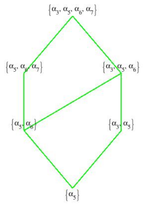
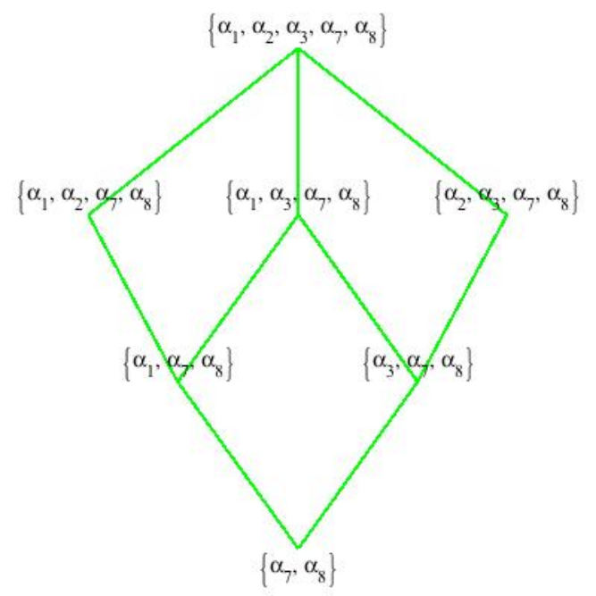
Refer to caption — Figure 3.1. Some non-atomic subintervals.

( $\Leftarrow$ ) We prove the converse statement. Let $\phi(e)\subseteq A\subseteq\phi(f)$ be an arbitrary subset. Let $\beta\in A-\phi(e)$ be a simple root. Hence, by hypotheses, either $\beta\notin J_{0}$ or $\beta\in J_{0}$ and $\sigma_{\alpha^{\prime}}\sigma_{\beta}=\sigma_{\beta}\sigma_{\alpha^{\prime}}$ for some $\alpha^{\prime}\in\phi(e)$ . In both of these cases, we see that $\phi(e)\cup\{\beta\}\in\phi(\Lambda^{*})$ . But we can repeat this for all elements of $A-\phi(e)$ . Therefore, $A\in\phi(\Lambda^{*})$ . This shows that the interval $[e,f]$ is isomorphic to the Boolean lattice $2^{\phi(f)-\phi(e)}$ which is relatively complemented, of course. This finishes the proof.

The second part of the proof the Theorem shows that

Corollary 3.6.

An interval of $\Lambda^{*}$ is relatively complemented if and only if atomic if and only if isomorphic to a Boolean lattice.

As an application we rewrite the Theorem 1.4

Corollary 3.7.

Let $\Lambda$ be a cross section lattice of an $J-$ irreducible monoid. Let $e\leq f$ be in $\Lambda$ . Then,

(3.8)

\mu(e,f)=\begin{cases}(-1)^{rk(f)-rk(e)}&\text{if}\ [e,f]\ \text{is a Boolean lattice},\\ 0&otherwise.\end{cases}

4. Flag symmetric cross section lattices

Recall that a poset is called flag-symmetric if and only if the flag-quasi symmetric function $F_{P}$ is a symmetric function. In this section we answer (at least, partially) the following question:

Which $J$ -irreducible monoids do have their cross section lattice flag-symmetric?

The following observation of Stanley is useful for deciding when a distributive lattice is flag-symmetric.

Theorem 4.1.

(Stanley, [23]) Let $L$ be a finite distributive lattice. The following four conditions are equivalent.

(1)

$L$ is locally self dual.
(2)

$L$ is locally rank-symmetric.
(3)

$L$ is flag-symmetric.
(4)

$L$ is a product of chains.

Remark 4.2.

Let $e_{0}$ be the minimal nonzero idempotent of $\Lambda$ , let $\Delta$ be a set of simple roots and let $J_{0}=\{\alpha\in\Delta|\ \sigma_{\alpha}e_{0}=e_{0}\sigma_{\alpha}\}$ be as before. In [10] Putcha and Renner observed that $\Lambda^{*}$ is a distributive lattice if and only if $\Delta-J_{0}$ is a connected subset of the Dynkin diagram of $G$ (in the sense of the Definition 3.4). In Figure 4.1 we have depicted some distributive cross section lattices. The example in Figure 6.1, however, is not distributive. For more examples see Renner’s book [17].

We are going to show that a distributive cross section lattice has to be a product of chains. In order to use Stanley’s theorem, however, we need to further analyze the structure of $\Lambda^{*}$ . We start by strengthening the observation of Putcha and Renner about the distributivity of the cross sections.

Proposition 4.3.

Let $J_{0}$ and $\Lambda$ be as in Theorem 1.3. The followings are equivalent

(1)

$\Lambda^{*}$ is isomorphic to a sublattice of the Boolean lattice of all subsets of $\Delta$ .
(2)

$\Lambda^{*}$ is distributive.
(3)

$\Delta-J_{0}$ is connected.

Proof.

By Remark 4.2 the equality of the second and third items is already known. Recall also that $\Lambda^{*}$ is closed under union operation. Therefore, it is enough to prove that $\Lambda^{*}$ is closed under intersections.

The $J_{0}$ consists of one or two connected subsets of $\Delta$ . We first assume that it has a single connected piece. Without loss of generality we may assume that $|\Delta|=n$ and that $J_{0}=\{\alpha_{1},...,\alpha_{k}\}$ for some $k<n$ such that $\sigma_{\alpha_{i}}\sigma_{\alpha_{i+1}}\neq\sigma_{\alpha_{i+1}}\sigma_{\alpha_{i}}$ for $i=1,...,k-1$ . Let $I_{1}\subseteq\Delta$ be such that no connected component of $I_{1}$ lie entirely in $J_{0}$ . Therefore, either $I_{1}\cap J_{0}=\emptyset$ , or $I_{1}\cap J_{0}=\{\alpha_{i},\alpha_{i+1},...,\alpha_{k}\}$ and $\alpha_{k+1}\in I_{1}$ . Let $I_{2}\subseteq\Delta$ be another such subset. Then, either $I_{1}\cap I_{2}\cap J_{0}$ is empty (hence there is nothing to prove), or $I_{1}\cap I_{2}\cap J_{0}=\{\alpha_{j},\alpha_{j+1},...,\alpha_{k}\}$ , for some $j\leq k$ , and $\alpha_{k+1}\in I_{1}\cap I_{2}$ . In other words, no connected component of $I_{1}\cap I_{2}$ lie entirely in $J_{0}$ . Hence, in this case, $\Lambda^{*}$ is closed under intersections.

Next, we assume that $\Lambda-J_{0}=\{\alpha_{i}:\ k\leq i\leq l\}$ for some $1\leq k<l\leq n$ . Let $I_{1}$ and $I_{2}$ be two subsets of $\Delta$ such that no connected components lie entirely in $J_{0}$ . Without loss of generality we may assume that $I_{1}\cap I_{2}\cap J_{0}\neq\emptyset$ . Then, either $I_{1}\cap I_{2}\cap\{\alpha_{l},\alpha_{l+1},...,\alpha_{n}\}=\emptyset$ , or $I_{1}\cap I_{2}\cap\{\alpha_{l},\alpha_{l+1},...,\alpha_{n}\}\neq\emptyset$ and $I_{1}\cap I_{2}\cap\{\alpha_{1},\alpha_{2},...,\alpha_{k}\}\neq\emptyset$ . In both of these cases we may proceed as in the previous paragraph. Therefore, $I_{1}\cap I_{2}$ has no connected component lying entirely in $J_{0}$ . Hence, $\Lambda^{*}$ is closed under intersections.

∎

Remark 4.4.

A distributive lattice is always modular, but the converse does not need to be true. A modular lattice is distributive if and only if it does not contain any interval of rank three which is isomorphic to a “diamond,” $M_{3}=\{a,b,c,d,e,f\}$ with $a<b,c,d$ and $b,c,d<e$ . (See Grätzer, [6] ).

Theorem 4.5.

Let $\Lambda$ be a modular cross section lattice, and let $J_{0}\subseteq\Delta$ be as before. If $|\Delta-J_{0}|>1$ , then every interval of rank three in $\Lambda^{*}$ is locally rank symmetric. If $|\Delta-J_{0}|=1$ , then every interval of rank three in $\Lambda^{*}-\{e_{0}\}$ is locally rank symmetric.

Proof.

The second assertion can be checked from the Fig. 2 of [10]. We are going to prove the first assertion. If $|\Delta-J_{0}|=2$ , then the first assertion can be checked from Fig. 7.1. of [17]. Therefore, we assume that $|\Delta-J_{0}|>2$ .

It is enough to prove that this for $J_{0}=\{\alpha_{1},...,\alpha_{k}\}$ , where $\alpha_{i}\alpha_{i+1}\neq\alpha_{i+1}\alpha_{i}$ for $i=1,...,k-1$ . (The case $J_{0}=\{\alpha_{l},...,\alpha_{n}\}$ is identical, and the case $J_{0}=\{\alpha_{1},...,\alpha_{k},\alpha_{l},...,\alpha_{n}\}$ is similar.)

It is convenient to identify $\Lambda^{*}$ by its image in $2^{\Delta}$ . Let $[U,V]\subseteq 2^{\Delta}$ be an interval of rank 3. Let $V=U\cup\{\alpha_{x},\alpha_{y},\alpha_{z}\}$ for some $x<y<z$ from $\{1,...,n\}$ .

If $\{\alpha_{x},\alpha_{y},\alpha_{z}\}\cap J_{0}\subseteq\{\alpha_{x}\}$ , then $[U,V]$ is isomorphic to the Boolean lattice of subsets of $\{x,y,z\}$ , which is locally rank symmetric. Thus, we may assume that $\{\alpha_{x},\alpha_{y}\}\subseteq\{\alpha_{x},\alpha_{y},\alpha_{z}\}\cap J_{0}$ . Then $U\cup\{\alpha_{x}\}$ can not be of the form $\phi(f)$ for some $f$ covering $\phi(e)=U$ . In other words, $U\cup\{\alpha_{x}\}$ is not contained in the interval $[U,V]$ . By the same token, $U\cup\{\alpha_{x},\alpha_{z}\}$ cannot be in $[U,V]$ .

If, in addition, $\alpha_{z}\in J_{0}$ , then neither $U\cup\{\alpha_{y}\}$ nor $U\cup\{\alpha_{x},\alpha_{y}\}$ can be in $[U,V]$ . In this case, $[U,V]=\{U,U\cup\{\alpha_{z}\},U\cup\{\alpha_{y},\alpha_{z}\},U\cup\{\alpha_{x},\alpha_{y},\alpha_{z}\}=V\}$ is a chain, and hence locally rank symmetric. If $\alpha_{z}\notin J_{0}$ , then $[U,V]=\{U,U\cup\{\alpha_{y}\},U\cup\{\alpha_{z}\},U\cup\{\alpha_{x},\alpha_{y}\},U\cup\{\alpha_{y},\alpha_{z}\},U\cup\{\alpha_{x},\alpha_{y},\alpha_{z}\}=V\}$ which is also locally rank symmetric.

This finishes the proof. ∎

The proof of the theorem gives the proof of the following corollary, also.

Corollary 4.6.

Let $\Lambda$ be a distributive (hence modular) cross section lattice of a $J-$ irreducible monoid of type $A_{n}$ . Let $J_{0}$ be as before. If $|\Delta-J_{0}|>1$ , then every interval of rank three in $\Lambda^{*}$ is isomorphic to one of the followings.

(1)

$2^{\{a,b,c\}}$ , the Boolean lattice on three letters.
(2)

$\{a,b,c,d,e,f\}$ where $a<b,\ a<c,\ b<d,\ c<d,\ c<e,\ e<f,\ d<f$ .
(3)

$\{a,b,c,d\}$ where $a<b<c<d$ .

Theorem 4.7.

(F. Regonati, [15]) Let $L$ be a finite modular lattice. The following three conditions are equivalent.

(1)

$L$ is locally rank symmetric.
(2)

Every interval of $L$ of rank three is rank-symmetric.
(3)

$L$ is a product $P_{1}\times P_{2}\times\cdots\times P_{m}$ of $q_{i}$ –primary lattices $P_{i}$ (including the possibility $q_{i}=0$ , in which case $P_{i}$ is a chain.

Corollary 4.8.

Let $\Lambda$ be a distributive (hence modular) cross section lattice of a $J-$ irreducible monoid of type $A_{n}$ . Let $e_{0}\in\Lambda$ and $J_{0}\subseteq\Delta$ be as before. If $|\Delta-J_{0}|>1$ , then $\Lambda^{*}$ is locally rank symmetric and is isomorphic to a product of chains. If $|\Delta-J_{0}|=1$ , then $\Lambda^{*}-\{e_{0}\}$ is locally rank symmetric and is isomorphic to a product of chains.

(a)

J_{0}=\{\alpha_{1},\alpha_{2},\alpha_{5}\}

(b)

J_{0}=\{\alpha_{1},\alpha_{2},\alpha_{3}\}

(c)

J_{0}=\{\alpha_{1},\alpha_{5}\}

(d)

J_{0}=\{\alpha_{1},\alpha_{2}\}

Figure 4.1. Some distributive cross section lattices for

\Delta=\{\alpha_{1},...,\alpha_{5}\}

Definition 4.9.

Let $\gamma=\gamma_{1}+\cdots+\gamma_{l}$ be a partition (of a composition), and let $L_{\gamma}$ be the product $C_{\gamma_{1}}\times\cdots\times C_{\gamma_{l}}$ of chains $C_{\gamma_{i}}$ of length $\gamma_{i}-1$ . We call $\gamma$ , the partition type of $L_{\gamma}$ .

It is easy to see that the flag quasi-symmetric function $F_{L_{\gamma}}$ of $L_{\gamma}=C_{\gamma_{1}}\times\cdots\times C_{\gamma_{l}}$ is equal to the complete homogenous symmetric function $h_{\gamma}=h_{\gamma_{1}}\cdots h_{\gamma_{l}}$ (see Proposition 3.3, [23]).

It is easy to see that the partition types of the distributive cross section lattices in Figure 4.1 are $(3,2),(4,1),(2,2,1)$ and $(3,1,1)$ in the given order of the figures (a),(b),(c) and (d). Notice that these are partitions of 5. In fact, it is easy to see that, for $n\leq 6$ the number of distinct distributive cross section lattices associated with $GL_{n}$ is equal to number of partitions of $n-1$ . Unfortunately this is not a general fact. The number of distinct distributive cross section lattices associated with $GL_{7}$ is 10, but the number of partitions of 6 is 11. This reminds us the curious phenomena of ungradedness of the dominance partial order on partitions for $n\geq 6$ .

Remark 4.10.

Note that the Conjecture 1.10 gives the possible “partition types” of the distributive cross section lattices; possible they are of the form $(k+1,n-l+2,1,1...,1)$ , $k\geq 0,\ l\geq 0$ .

4.0.1. Combinatorially smooth subsets of $W$

An important result of Renner says that, when $M$ is $J$ -irreducible monoid, the poset of idempotents of the (maximal) torus embedding $E(\overline{T})$ is isomorphic to the face lattice of the polytope $Conv(W\cdot\mu)$ , where $\mu$ is the highest weight associated with the defining irreducible representation of $M$ .

The set of nonzero minimal elements in $E(\overline{T})$

E_{1}(\overline{T})=\{e\in E(\overline{T}):\ \dim(Te)=1\}

plays a special role in Renner’s descent sysyems (see [18]).

Definition 4.11.

Let $e,e^{\prime}\in E_{1}(\overline{T})$ be two different minimal, nonzero idempotents. We write $e<e^{\prime}$ whenever $eBe^{\prime}\neq 0$ .

To be consistent with Renner’s notation from [18], in this section, we let $e_{1}$ denote the minimal nonzero idempotent of $\Lambda$ .

Theorem 4.12.

(Renner, [18]) The followings are equivalent for $v,w\in W^{J}$ .

(1)

$e=ve_{1}v^{-1}<e^{\prime}=we_{1}w^{-1}$ in $(E_{1},<)$
(2)

$w<v$ in $(W^{J},<)$ in the Bruhat ordering on $W^{J}$ .

It is implicit in this theorem that $E_{1}(\bar{T})$ can be identified with $W^{J}$ . This follows from (2.17) and the fact that $M$ is $J-$ irreducible. Recall that $J$ is called combinatorially smooth if the toric variety associated with the polytope $Conv(W\cdot\mu)$ is rationally smooth.

The reader can extend the following observation to other types:

Proposition 4.13.

Let $\Delta$ be a set of simple roots of type $A_{n}$ , $n\geq 2$ . Then, a subset $J\subseteq S=\{\sigma_{\alpha}:\ \alpha\in\Delta\}$ of the simple reflections is combinatorially smooth if and only if $\Lambda^{*}$ (defined by $J_{0}=J$ ) is distributive and one of the followings hold:

a)

$|\Delta-J|\geq 1$ , if $J$ contains only one of the end nodes of the Dynkin diagram,
b)

$|\Delta-J|\geq 2$ , if $J$ contains both ends of the Dynkin diagram.

Proof.

See Corollary 3.5 in [18]. ∎

5. Supersolvability

In this section we find a necessary and sufficient condition for a cross section lattice of a $J-$ irreducible to be supersolvable. We assume for this section that all the cross section lattices belong to one of the following types $A_{n},B_{n}$ or $C_{n}$ .

Definition 5.1.

A finite lattice $L$ is called supersolvable if it possesses a maximal chain $\varGamma$ , called modular chain or $\mathcal{M}-chain$ , with the property that the sublattice of $L$ generated by $\varGamma$ and any other chain of $L$ is distributive.

Recall that an element $b\in L$ of a lattice is called right modular if and only if for every $a\in L$

(5.2)

c\leq b\Rightarrow c\vee(a\wedge b)=(c\vee a)\wedge b.

Similarly, $a\in L$ is called left modular if and only if for every $b\in L$ , (5.2) holds. An element $a\in L$ is called modular if it is both right and left modular.

The following characterization of semismodular supersolvable lattices is useful.

Lemma 5.3.

(Stanley, Corollary 2.3, [22]) Let $L$ be a finite upper semimodular lattice, and $\varGamma$ be a maximal chain of $L$ . Then, $\varGamma$ is a modular chain if and only if every element of $\varGamma$ is modular.

To prove the Theorem 1.11 we need the followings, as well:

Lemma 5.4.

Let $X$ be the image $\phi(e)\in\phi(\Lambda)$ of an idempotent under the map $\phi:\Lambda\rightarrow 2^{\Delta}$ of the Theorem 1.3. If $X\cap J_{0}=\emptyset$ , then $e$ is both right and left modular.

Proof.

By abuse of notation, using the map $\phi$ of the Theorem (1.3), we identify $\Lambda$ by its image. (Therefore, if $h\leq f$ in $\Lambda$ and $Z=\phi(h),\ Y=\phi(f)$ , then we write $Z\leq Y$ .) Let $X=\phi(e)$ be as in the hypotheses: $X\cap J_{0}=\emptyset$ .

We first show that $X$ is right modular. Let $U$ and $V$ be two subsets from $\Lambda$ such that $V\leq X$ . Using Corollary 3.2 $U\wedge X=U\cap X$ , and there exists $H\in\Lambda$ such that $U\cap X=H$ . Since $V\vee H=V\cup H$ , $V\vee(U\wedge X)=V\cup(U\cap X)$ . Since $V\subseteq X$ we see that $V\cup(U\cap X)=(V\cup U)\cap X$ . On the other hand the right hand side of the last equality is $(V\vee U)\wedge X$ . Hence for $U,V\in\Lambda$ such that $V\leq X$ the implication in (5.2) holds. In other words, $X$ is a right modular element of $\Lambda$ .

Next, we show that $X$ is left modular. We need to show that for every $V\in\Lambda$ and $U\leq V$ ,

(5.5)

U\vee(X\wedge V)=(U\vee X)\wedge V.

By the Corollary 3.2, the left hand side of the Equation (5.5) is equal to $U\cup(X\cap V)$ , and $(U\vee X)=(U\cup X)$ . Hence, $(U\vee X)\wedge V\subseteq(U\cup X)\cap V$ . Therefore, it is enough to prove that $(U\cup X)\cap V\subseteq(U\vee X)\wedge V$ . To this end, let $\alpha\in(U\cup X)\cap V$ . If $\alpha\notin J_{0}$ , then $J_{0}$ cannot contain the connected component of $\alpha$ , so $\alpha\in(U\vee X)\wedge V$ . Therefore, we may assume that $\alpha\in J_{0}$ . It follows that $\alpha\in U\subseteq V$ . Therefore, connected component of $\alpha$ in $(U\cup X)\cap V$ is at least as large as the connected component of $\alpha\in U$ . In other words, $J_{0}$ cannot contain the connected component of $\alpha$ , and hence $\alpha\in(U\vee X)\wedge V$ . This finishes the proof.

∎

Lemma 5.6.

Suppose that a connected component of $J_{0}$ is either a singleton $\{\alpha_{i}\}$ , $\alpha_{i}\in\Delta$ , or is of the form $\widetilde{J_{0}}=\{\alpha_{i_{1}},\alpha_{i_{2}},...,\alpha_{i_{k}}\}\subseteq J_{0},\ k>1$ such that

(1)

if $\alpha_{i_{k}}\in\widetilde{J_{0}}$ , then there exists $\alpha_{i_{l}}\in\widetilde{J_{0}}$ such that $\sigma_{\alpha_{i_{k}}}\sigma_{\alpha_{i_{l}}}\neq\sigma_{\alpha_{i_{l}}}\sigma_{\alpha_{i_{k}}}$ , and
(2)

there exists an end-node $\alpha_{i}$ of $\Delta$ contained in $\widetilde{J_{0}}$ .

Let $X=\phi(e)\in\phi(\Lambda)$ be such that $\Delta-J_{0}\subseteq X$ . Then, $e$ is both right and left modular.

Proof.

We proceed as in the proof of the Lemma 5.4, using the map $\phi$ of the Theorem (1.3) to identify $\Lambda$ by its image. Let $X$ be as in the hypotheses, so that $\Delta-J_{0}\subseteq X$ . Notice if we can show that for every $U\in\Lambda$ , $U\wedge X=U\cap X$ , then we are done by the proof of the Lemma 5.4.

To this end, we assume that there exists $U\in\Lambda$ such that $U\wedge X\neq U\cap X$ . Thus, by Corollary 3.2, there must exist $\alpha\in J_{0}\cap U\cap X$ with a connected neighborhood (in $U\cap X$ ) which lies completely in $J_{0}$ . Since $\Delta-J_{0}\subseteq X$ , if $\{\alpha\}\in J_{0}$ is a singleton subset of $J_{0}$ , any connected component of $U$ which contains $\alpha$ has to intersect $X$ with more than one element. In other words, the connected component in $U\cap X$ of $\alpha$ cannot lie in $J_{0}$ completely. If $\alpha$ lies in a component $\widetilde{J_{0}}$ of $J_{0}$ which contains an end-node, then we proceed as in the proof the Proposition 4.3. Suppose that $\widetilde{J_{0}}=\{\alpha_{j_{1}},\alpha_{j_{2}},...,\alpha_{j_{k}}\}$ is the connected subset $J_{0}$ containing $\alpha$ , and $\alpha_{j_{k}}\in\widetilde{J_{0}}$ is an end-node (of $\Delta$ ).

Then, $U\cap J_{0}=\{\alpha_{j_{1}},\alpha_{j_{2}},...,\alpha_{j_{l}}\}$ , for some $l\leq k$ such that $\sigma_{\alpha_{j_{m}}}\sigma_{\alpha_{j_{m+1}}}\neq\sigma_{\alpha_{j_{m+1}}}\sigma_{\alpha_{j_{m}}}$ for $m=1,...,l-1$ . Furthermore, there exists $\alpha^{\prime}\in U-J_{0}$ such that $\sigma_{\alpha^{\prime}}\sigma_{\alpha_{j_{1}}}\neq\sigma_{\alpha_{j_{1}}}\sigma_{\alpha^{\prime}}$ .

Since $\Delta-J_{0}\subseteq X$ , $\alpha^{\prime}\in X$ . Therefore, $\{\alpha^{\prime}\}\cup U\cap J_{0}\subseteq X$ , and hence, no connected component of $\alpha$ in $U\cap X$ can lie completely in $J_{0}$ . In other words, $U\cap X=U\wedge X$ . The rest of the proof goes as in the previous Lemma 5.4. ∎

Proof of Theorem 1.11. ( $\Leftarrow$ ) We explicitly construct an $\mathcal{M}$ -chain. Once again, we identify $\Lambda$ with its image in $2^{\Delta}$ . Let $J_{0}=\{\alpha_{i_{1}},\alpha_{i_{2}},...,\alpha_{i_{k}}\}\subseteq\Delta$ be as in the hypotheses of the Theorem 1.11, and let $\{\alpha_{j_{1}},...,\alpha_{j_{m}}\}$ be the complement of $J_{0}$ in $\Delta$ . We assume that $i_{1}<i_{2}<\cdots<i_{k}$ , and $j_{1}<j_{2}<\cdots<j_{m}$ .

By Corollary 3.2, any entry $U$ of the chain

\emptyset\subset\{\alpha_{j_{1}}\}\subset\{\alpha_{j_{1}},\alpha_{j_{2}}\}\subset\cdots\subset\{\alpha_{j_{1}},...,\alpha_{j_{m}}\}

is an element of $\Lambda$ , and furthermore, by Lemma 5.4, $U$ is both left and right modular.

Let $I=\{i_{1},...,i_{k^{\prime}}\}\subseteq[k]$ be the set of indices of elements of $J_{0}$ which are less than $j_{1}$ . The set $I$ might be empty. If not, by the hypotheses of the Theorem, $\{i_{1},...,i_{k^{\prime}}\}=\{1,...,k^{\prime}\}$ . Then, it is easy to check that the entries of the chain

(5.7)

\{\alpha_{i_{k^{\prime}}}\}\cup(\Delta-J_{0})\subset\cdots\subset\{\alpha_{i_{1}},\alpha_{i_{2}},\ldots,\alpha_{i_{k^{\prime}}}\}\cup(\Delta-J_{0})

as well as the entries of the chain

(5.8)

U_{i_{k^{\prime}+1}}\subset U_{i_{k^{\prime}+2}}\subset\cdots\subset U_{i_{k}}=\Delta,

where

	$\displaystyle U_{i_{k^{\prime}+1}}$	$\displaystyle=\{\alpha_{i_{1}},...,\alpha_{i_{k^{\prime}}}\}\cup(\Delta-J_{0})\cup\{\alpha_{i_{k^{\prime}+1}}\}$
	$\displaystyle U_{i_{k^{\prime}+2}}$	$\displaystyle=\{\alpha_{i_{1}},...,\alpha_{i_{k^{\prime}}}\}\cup(\Delta-J_{0})\cup\{\alpha_{i_{k^{\prime}+1}},\alpha_{i_{k^{\prime}+2}}\}$

	$\displaystyle U_{i_{k}}$	$\displaystyle=\{\alpha_{i_{1}},...,\alpha_{i_{k^{\prime}}}\}\cup(\Delta-J_{0})\cup\{\alpha_{i_{k^{\prime}+1}},\alpha_{i_{k^{\prime}+2}},\ldots,\alpha_{i_{k}}\}$

are in $\Lambda$ .

By Lemma 5.6, any entry of the chain (5.7) and any entry of (5.8) is both left and right modular. Therefore, we have found a maximal chain $\varGamma$ whose entries are both left and right modular.

( $\Rightarrow$ ) Assume $\Lambda$ is supersolvable and that there exists a connected component $\widetilde{J_{0}}\subseteq J_{0}$ which does not contain an end-node of $\Delta$ , and $|\widetilde{J_{0}}|>1$ , say $\widetilde{J_{0}}=\{\alpha_{i_{1}},...,\alpha_{i_{k}}\}$ , $k>1$ . Then, there exist $\alpha,\alpha^{\prime}\in\Delta-J_{0}$ such that $\sigma_{\alpha}\sigma_{\alpha_{i_{1}}}\neq\sigma_{\alpha_{i_{1}}}\sigma_{\alpha}$ , and $\sigma_{\alpha^{\prime}}\sigma_{\alpha_{i_{k}}}\neq\sigma_{\alpha_{i_{k}}}\sigma_{\alpha^{\prime}}$ . Let $\varGamma$ be a modular chain for $\Lambda$ . Then, there exist an entry $\varGamma_{t}$ of $\varGamma$ such that there exists $\alpha_{i_{m}}\in\widetilde{J_{0}}-\varGamma_{t}$ for some $1\leq m<k$ . Without loss of generality we may assume that $\alpha_{i_{n}}\in\varGamma_{t}$ whenever $m<n\leq k$ . Let $C$ be the subset $\{\alpha_{i_{m+2}},...,\alpha_{k},\alpha^{\prime}\}\subseteq\varGamma_{t}$ . Let $A$ be the set $\{\alpha,\alpha_{i_{1}},...,\alpha_{i_{m}},\alpha_{i_{m+1}}\}$ . Clearly, $A$ and $C$ are in $\Lambda$ . Since $\alpha_{i_{m+1}}\in A\cap\varGamma_{t}$ is isolated in $J_{0}$ , $A\wedge\varGamma_{t}$ cannot contain $\alpha_{i_{m+1}}$ . Therefore, $\alpha_{i_{m+1}}\notin C\vee(A\wedge\varGamma_{t})$ . However, it is easy to check that $\alpha_{i_{m+1}}\in(C\vee A)\wedge\varGamma_{t}$ . In other words,

C\vee(A\wedge\varGamma_{t})\neq(C\vee A)\wedge\varGamma_{t}.

Therefore, the element $\varGamma_{t}$ of the modular chain $\varGamma$ is not (right) modular, which contradicts with the Lemma 5.3. Therefore, we must have $|\widetilde{J_{0}}|\leq 1$ . This finishes the proof.

6. Characteristic polynomials

Recall that the Möbius function of a poset $P$ is the unique function $\mu:P\times P\rightarrow{\mathbb{N}}$ satisfying

(1)

$\mu(x,x)=1$ for every $x\in P$ ,
(2)

$\mu(x,y)=0$ whenever $x\nleq y$ ,
(3)

$\mu(x,y)=-\sum_{x\leq z<y}\mu(x,z)$ for all $x<y$ in $P$ .

The characteristic polynomial $p(\alpha,P)$ (also known as Birkhoff polynomial) of a finite graded poset $P$ of rank $n$ is

(6.1)

p(x,P)=\sum_{x\in P}\mu(\hat{0},x)x^{rk(\hat{1})-rk(\hat{x})}.

A particularly nice survey about characteristic polynomials is written by B. Sagan and can be found at [19].

Conjecture 6.2.

Let $\Lambda$ be the cross section lattice of a $J-$ irreducible monoid $M$ . Then

(6.3)

p(x,\Lambda^{*})=x^{|J_{0}|}(x-1)^{n-|J_{0}|}.

In this section we prove the following following special case of the above conjecture.

Theorem 6.4.

Let $n$ be the rank of the supersolvable cross section lattice $\Lambda^{*}$ . Then the characteristic polynomial of $\varGamma$ is

(6.5)

p(x,\Lambda^{*})=x^{|J_{0}|}(x-1)^{n-|J_{0}|}.

Proof.

Recall Theorem 1.13: If $L$ be a semimodular supersolvable lattice and $\hat{0}=x_{0}<x_{1}<\cdots<x_{n}=\hat{1}$ is an $\mathcal{M}$ -chain, then

(6.6)

p(x,L)=(x-a_{1})(x-a_{2})\cdots(x-a_{n}),

where $a_{i}$ is the number of atoms $u\in L$ such that $u\leq x_{i}$ and $u\nleq x_{i-1}$ .

In the proof of Theorem 1.11 we found an $\mathcal{M}$ -chain $D$ . It is easy to check that $\Delta-J_{0}$ is the set of atoms of $\Lambda^{*}$ . Furthermore, initial part $x_{0}=\hat{0}<x_{1}<\cdots<x_{k}$ of $D$ is given by the subsets $x_{s}=\{j_{1},...,j_{s}\}_{<}\subseteq\Delta-J_{0}$ . Therefore, $a_{s}=1$ for $s=1,...,|\Delta-J_{0}|$ . Since $x_{s}\subseteq x_{r}$ for $s<r$ , it follows that $a_{r}=0$ . Therefore,

(6.7)

p(x,\Lambda^{*})=\prod_{s=1}^{|\Delta-J_{0}|}(x-1)\prod_{r=|\Delta-J_{0}|+1}^{|\Delta|}x=x^{|J_{0}|}(x-1)^{n-|J_{0}|}.

This finishes the proof.

∎

The monoid in the following example is interesting in its own right.

Example 6.8.

Let $\Lambda$ be the cross section lattice of the monoid obtained from $SL_{5}$ by using the adjoint representation $\rho(g)=\text{Ad}(g)$ . Then, one can show that $J_{0}=\{\alpha_{2},\alpha_{3}\}\subseteq\Delta=\{\alpha_{1},\alpha_{2},\alpha_{3},\alpha_{4}\}$ . The Hasse diagram of $\Lambda^{*}$ is as in Figure 6.1 (see also Section 7.4.1. of [17]). By Theorem 1.11, $\Lambda^{*}$ is not supersolvable, however, a straightforward calculations shows that the characteristic polynomial of $\Lambda^{*}$ is equal to $x^{2}(x-1)^{2}$ .

Figure 6.1. The cross section lattice of an adjoint representation.

7. Future directions

In this section, we briefly report some of our progress as a continuation of the results of this article. However, we take the liberty of not introducing the further notation.

In [8], McNamara shows that a lattice $L$ is supersolvable if and only if there exists a 0-Hecke algebra action on the maximal chains of the lattice $L$ . He furthermore shows that under a suitable analogue of the Frobenius characteristic map, the representations on the maximal chains might be identified with the flag quasi symmetric functions studied by Stanley (see Section 2.1, and [23]). We will write our progress on the representations of the 0-Hecke algebra on $\Lambda^{*}$ in a forthcoming article. However, we would like to mention that, in general, flag quasi symmetric functions of Stanley are nice for a cross section lattice of a $J-$ irreducible monoid. To give the flavor of the results in that direction we state without a proof the following observation:

Let $\langle,\rangle$ be the nondegenerate inner product on the space of quasi symmetric functions such that the set $\{F_{I,n}:\ I\subseteq\{1,...,n-1\}\}$ of fundamental quasi symmetric functions forms an orthonormal basis.

Theorem 7.1.

Let $\Lambda^{*}$ be a rank $n$ cross section a $J-$ irreducible monoid. Let $J_{0}\subseteq\Delta$ be as in Theorem 1.3, and let $n=|\Delta|$ .Then,

\langle F_{\Lambda^{*}},F_{\{1\},n}\rangle=|n-J_{0}|.

The NilCoxeter algebra of a Weyl group plays an important role in the theory of symmetric functions, especially in type $A_{n}$ . We can show that, like a 0-Hecke algebra, the nilCoxeter algeba acts on the maximal chains of $\Lambda^{*}$ , also. Thereby, we apply the work of S. Fomin and C. Greene, [5]. This enables us to generalize Stanley symmetric functions, as well as stable Grothendieck polynomials (via 0-Hecke algebra action) to the setting of the cross section lattices. We will report on these considerations in future papers.

7.1. Variation of the theme

As a result of Theorem 1.3, the following definition of a “combinatorial cross section lattice” is appropriate:

Definition 7.2.

Let ${\mathcal{G}}$ be a graph. By abuse of notation we use ${\mathcal{G}}$ to denote the set of vertices as well (thus $2^{G}$ is the set of all subsets of the vertex set ${\mathcal{G}}$ ). Let $J_{0}\subseteq{\mathcal{G}}$ be a subset of the vertex set. The combinatorial cross section lattice $\Lambda=\Lambda({\mathcal{G}},J_{0})\subseteq 2^{\mathcal{G}}$ associated with the pair $({\mathcal{G}},J_{0})$ consists of those subsets $U\in 2^{\mathcal{G}}$ having no connected component contained entirely in $J_{0}$ as an induced subgraph. The partial ordering on $\Lambda$ is the set inclusion. We consider the empty set as an element of $\Lambda$ .

Remark 7.3.

It is clear that if $U$ and $V$ are from a combinatorial cross section poset $\Lambda$ , then the join $U\vee V\in\Lambda$ exists and equal to the union $U\cup V$ . If $U\cap V$ is an element of $\Lambda$ , then it is equal to the meet $U\wedge V$ , otherwise the meet is equal to $\emptyset\in\Lambda$ .

Obviously, when ${\mathcal{G}}$ is the graph ${\mathcal{G}}=\{\alpha_{1},\ldots,\alpha_{n}\}$ with the edge set $E=\{e_{1},\ldots,e_{n-1}\}$ , where $e_{i}$ connects $\alpha_{i}$ and $\alpha_{i+1}$ an associated combinatorial cross section lattice is equal to a cross section lattice of a $J$ -irreducible monoid of type $A_{n}$ , considered in the manuscript.

We are planning to investigate the case of an arbitrary graph in a future paper. However, let us mention here briefly the case when ${\mathcal{G}}$ is a circuit. In other words, the (Coxeter) graph of an affine root system of type $\tilde{A}_{n}$ . Its vertex set is ${\mathcal{G}}=\Delta_{af}=\Delta\cup\{\alpha_{0}\}$ , where $\Delta$ is a set of simple roots of type $A_{n}$ , and $\alpha_{0}$ is connected to both of the end nodes of $\Delta$ .

Theorem 7.4.

Let ${\mathcal{G}}$ be a circuit, and let $J_{0}\subseteq{\mathcal{G}}$ .

(1)

If ${\mathcal{G}}-J_{0}$ contains (at least) two adjacent vertices, then $\Lambda({\mathcal{G}},J_{0})$ is isomorphic to a cross section lattice of a $J$ -irreducible monoid of type $A$ .
(2)

${\mathcal{G}}$ is supersolvable if and only if each connected component of $J_{0}$ is a singleton.

Proof.

(1)

Suppose that the vertex set of ${\mathcal{G}}$ is $\{\beta_{0},\beta_{1},\ldots,\beta_{n}\}$ and its edge set is $\{e_{0},\ldots,e_{n}\}$ where $e_{i}$ connects $\beta_{i}$ and $\beta_{i+1}$ , $i=0,\ldots,n-1$ , and $e_{n}$ connects $\beta_{n}$ and $\beta_{0}$ . Without loss of generality we may assume that $\beta_{0}$ and $\beta_{1}$ are the two vertices which are not contained in ${\mathcal{G}}-J_{0}$ .

Let $\Delta$ be a root system (of type $A_{n+1}$ ) with the set of simple roots $\{\alpha_{1},\ldots,\alpha_{n+1}\}$ such that there exists an edge between $\alpha_{i}$ and $\alpha_{i+1}$ for $i=1,\ldots,n$ . Define

J_{0}^{\prime}=\{\alpha_{i}\in\Delta:\ \beta_{i}\in J_{0}\}

For $U\in\Lambda({\mathcal{G}},J_{0})$ define $\Phi(U)$ by

\alpha_{i}\in\Phi(U)\ \text{if}\ \begin{cases}i\neq n+1\ \text{and}\ \beta_{i}\in U,\\ i=n+1\ \text{and}\ \beta_{0}\in U.\end{cases}

Let $\Lambda$ be the cross section lattice of a $J$ -irreducible monoid on $\Delta$ determined by $J_{0}^{\prime}$ as in the Theorem 1.3. Then, it is easy to check that $U\mapsto\Phi(U)$ is an isomorphism between $\Lambda({\mathcal{G}},J_{0})$ and $\Lambda$ .

(2)

Similar to the proof of the Theorem 1.11.

∎

Remark 7.5.

It is easy to see that the proof of the first part of the Theorem 7.4 can be reversed to show that if $J_{0}^{\prime}\subseteq\Delta$ does not contain any of the end nodes of the diagram of $\Delta$ , then $\Lambda$ is isomorphic to a combinatorial cross section lattice $\Lambda({\mathcal{G}},J_{0})$ for some $J_{0}\subset{\mathcal{G}}$ , and ${\mathcal{G}}$ is a circuit.

References

[1] A. Björner, F. Brenti, Combinatorics of Coxeter groups, Springer-Verlag, New York, 2005.
[2] A. Björner, M. Wachs, Bruhat order of Coxeter groups and shellability, Adv. in Math. 43 (1982), no.1, 87–100.
[3] M.B. Can, The rook monoid is lexicographically shellable, Preprint (2008).
[4] R. Ehrenborg, On posets and Hopf algebras, Adv. Math. 119 (1997) 42–99.
[5] S. Fomin, C. Greene, Noncommutative Schur functions and their applications, Discrete Math. 193 (1998), no. 1-3, 179–200.
[6] G. Grätzer, General Lattice Theory, Second Ed., Birkhäuser-Verlag, Basel-Boston-Berlin, 1998.
[7] J. E. Humphreys, Linear Algebraic Groups, Springer-Verlag, New York, 1998.
[8] P. McNamara, EL-labelings, supersolvability and 0-Hecke algebra actions on posets, Journal of Com. Theory, Series A, 101 (2003) 69–89.
[9] R. Proctor, Classical Bruhat orders and lexicographic shellability, J. of Algebra, 77 (1982), no.1, 104–126.
[10] M.S. Putcha, L.E. Renner, The system of idempotents and the lattice of $J$ -classes of reductive algebraic monoids, Journal of Algebra, 116 (1988) 385–399.
[11] M.S. Putcha, Idempotent cross section lattices of $\mathcal{J}$ -classes, Semigroup Forum, 26 (1986) 103–109.
[12] M.S. Putcha, Linear Algebraic Monoids, London Math. Soc. Lecture Note Series, Cambridge University Press, Cambridge, 1988.
[13] M.S. Putcha, Shellability in reductive monoids, Tran. Amer. Math. Soc. 354 (2001), 413–426.
[14] M.S. Putcha, Möbius functions on cross section lattices, Journal of Combinatorial Theory, Series A, 106 (2004), 287–297.
[15] F. Regonati, Whitney numbers of the second kind of finite modular lattices, Journal of Combinatorial Theory, Series A, 60 (1992), 34–49.
[16] L.E. Renner, Classification of semisimple algebraic monoids, Trans. Amer. Math. Soc. 292 193–223 (1985).
[17] L.E. Renner, Linear Algebraic Monoids, Encyclopedia of Mathematical Sciences, Vol.134, Subseries: Invariant Theory, Vol.5, Springer-Verlag, 2005.
[18] L.E. Renner, Descent systems for Bruhat posets, Journal of Algebraic Combinatorics, 29 (2009), no. 4, 413–435.
[19] B. Sagan, Why the characteristic polynomial factors, Bulletin of AMS. Vol 36, no. 2 (1999), 113–133.
[20] A. Rittatore, Algebraic monoids and group embeddings, Transformation Groups, 3 (1998), 375–396.
[21] L. Solomon, An introduction to reductive monoids, “Semigroups, formal languages and groups”, J. Fountain, Ed., Kluwer Academic Publishers, (1995), 295–352.
[22] R.P. Stanley, Supersolvable lattices, Algebra Universalis 2 (1972), 197–217.
[23] R. P. Stanley, Flag-symmetric and locally rank-symmetric partially ordered sets, Electron. Journal of Combin. 3 (1996).
[24] R. P. Stanley, Enumerative Combinatorics, Volume 1, Cambridge Studies in Advanced Mathematics, 49. Cambridge University Press, Cambridge, 1997.
[25] R. P. Stanley, Enumerative Combinatorics, Volume 2, Cambridge Studies in Advanced Mathematics, 49. Cambridge University Press, Cambridge, 1997.

Supersolvable lattices of JJ-classes

Abstract.

1. Introduction

Theorem 1.3.

Theorem 1.4.

Theorem 1.6.

Corollary 1.8.

Theorem 1.9.

Conjecture 1.10.

Theorem 1.11.

Theorem 1.13.

Theorem 1.15.

Conjecture 1.17.

2. Preliminaries

2.1. Poset terminology

2.2. Reductive groups and monoids

3. The cross section of a J−J-irreducible monoid

Theorem 3.1.

Corollary 3.2.

Corollary 3.3.

Proof.

Definition 3.4.

Proposition 3.5.

Proof.

Corollary 3.6.

Corollary 3.7.

4. Flag symmetric cross section lattices

Theorem 4.1.

Remark 4.2.

Proposition 4.3.

Proof.

Remark 4.4.

Theorem 4.5.

Proof.

Corollary 4.6.

Theorem 4.7.

Corollary 4.8.

Definition 4.9.

Remark 4.10.

4.0.1. Combinatorially smooth subsets of WW

Definition 4.11.

Theorem 4.12.

Proposition 4.13.

Proof.

5. Supersolvability

Definition 5.1.

Lemma 5.3.

Lemma 5.4.

Proof.

Lemma 5.6.

Proof.

6. Characteristic polynomials

Conjecture 6.2.

Theorem 6.4.

Proof.

Example 6.8.

7. Future directions

Theorem 7.1.

7.1. Variation of the theme

Definition 7.2.

Remark 7.3.

Theorem 7.4.

Proof.

Remark 7.5.

References

Supersolvable lattices of $J$ -classes

3. The cross section of a $J-$ irreducible monoid

4.0.1. Combinatorially smooth subsets of $W$