On the Meaning of Mean Shape
Abstract
Various concepts of mean shape previously unrelated in the literature are brought into relation. In particular for non-manifolds such as Kendall’s 3D shape space, this paper answers the question, for which means one may apply a two-sample test. The answer is positive if intrinsic or Ziezold means are used. The underlying general result of manifold stability of a mean on a shape space, the quotient due to an isometric action of a compact Lie group on a Riemannian manifold, blends the Slice Theorem from differential geometry with the statistics of shape. For 3D Procrustes means, however, a counterexample is given. To further elucidate on subtleties of means, for spheres and Kendall’s shape spaces, a first order relationship between intrinsic, residual/Procrustean and extrinsic/Ziezold means is derived stating that for high concentration the latter approximately divides the (generalized) geodesic segment between the former two by the ratio . This fact, consequences of coordinate choices for the power of tests and other details, e.g. that extrinsic Schoenberg means may increase dimension are discussed and illustrated by simulations and exemplary datasets.
Key words and phrases: intrinsic mean, extrinsic mean, Procrustes mean, Schoenberg mean, Ziezold mean, shape spaces, compact Lie group action, slice theorem, horizontal lift, manifold stability
Figure AMS 2000 Subject Classification: Primary 60D05 Secondary 62H11
1 Introduction
The analysis of shape may be counted among the very early activities of mankind; be it for representation on cultural artefacts, or for morphological, biological and medical applications. In modern days shape analysis is gaining increased momentum in computer vision, image analysis, biomedicine and many other fields. For a recent overview cf. Krim and Yezzi (2006).
A shape space can be viewed as the quotient of a Riemannian manifold – e.g. the pre-shape sphere of centered unit size landmark configurations – modulo the isometric and proper action of a Lie group (cf. Bredon (1972)), conveying shape equivalence – e.g. the group of rotations, cf. (Kendall et al., 1999, Chapter 11). Thus, it carries the canonical quotient structure of a union of manifold strata of different dimensions, which give in general a Riemannian manifold part – possibly with singularities comprising the non-manifold part of non-regular shapes at some of which sectional curvatures may tend to infinity, cf. (Kendall et al., 1999, Chapter 7.3) as well as Huckemann et al. (2010b).
In a Euclidean space, there is a clear and unique concept of a mean in terms of least squares minimization: the arithmetic average. Generalizing to manifolds, however, the concept of expectation, average or mean is surprisingly non trivial and not at all canonical. In fact, it resulted in an overwhelming number of different concepts of means, each defined by a specific concept of a distance, all of which are identical for the Euclidean distance in a Euclidean space. More precisely, with every embedding in a Euclidean space come specific extrinsic and residual means and with every Riemannian structure comes a specific intrinsic mean. Furthermore, due to the non-Euclidean geometry, local minimizers introduced as Karcher means by Kendall (1990) may be different from global minimizers called Fréchet means by Ziezold (1977), and, neither ones are necessarily unique. Nonetheless, carrying statistics over to manifolds, strong consistency (by Ziezold (1977), Bhattacharya and Patrangenaru (2003)) and under suitable conditions, central limit theorems (CLTs) for such means have been derived (by Jupp (1988), Hendriks and Landsman (1996); Hendriks and Landsman (1998), Bhattacharya and Patrangenaru (2005) as well as Huckemann (2010a)). On shape spaces, various other concepts of means have been introduced, e.g. the famous Procrustes means (cf. Ziezold (1977),Dryden and Mardia (1998)). As we show here, these means are related to the above ones via a horizontal lifting from the bottom quotient to the top manifold, cf. Table 1. In particular, since there are many – and often confusing – variants of Procrustes means in the literatur this paper introduces the terminology of Procrustean means standing for inheritance from residual means.
For a CLT to hold, a manifold structure locally relating to a Euclidean space is sufficient. This leads to the question under which conditions it can be guaranteed that a mean shape lies on the manifold part.
Due to strong consistency, for a one-sample test for a specific mean shape on the manifold part, it may be assumed that sample means eventually lie on the manifold part as well, thus making the above cited CLTs available. To date however, a two- and a multi-sample test could not be justified because of a lacking result on the following manifold stability.
Definition 1.1.
A mean shape enjoys manifold stability if it is assumed on the manifold part for any random shape assuming the manifold part with non-zero probability.
A key result of this paper establishes manifold stability for intrinsic and Ziezold means under the following condition.
Condition 1.2.
On the non-manifold part the distribution of the random shape contains at most countably many point masses.
Since the non-manifold part is a null-set (e.g. Bredon (1972)) under the projection of the Riemannian volume, this condition covers most realistic cases.
We develop the corresponding theory for a general shape space quotient based on lifting a distribution on the shape space to the pre-shape space and subsequently exploiting the fact that intrinsic means are zeroes of an integral involving the Riemann exponential. The similar argument can be applied to Ziezold means but not to Procrustean means. More specifically, we develop the notion of a measurable horizontal lift of the shape space except for its quotient cut locus (introduced as well) to the pre-shape space. This requires the geometric concept of tubular neighborhoods admitting slices.
Curiously, the result applied to the finite dimensional subspaces exhausting the quotient shape space of closed planar curves with arbitrary initial point introduced by Zahn and Roskies (1972) and further studied by Klassen et al. (2004), gives that the shape of the circle, since it is a singularity, can never be an intrinsic shape mean of non-circular curves.
As a second curiosity, 3D full Procrustes means do not enjoy manifold stability in general, a counterexample involving low concentration is given. This is due to the fact that for low concentration, full Procrustes means may be ‘blinder’ in comparison to intrinsic and Ziezold means to distributional changes far away from a mode. Included in this context is also a discussion of the Schoenberg means, recently introduced by Bandulasiri and Patrangenaru (2005) as well as by Dryden et al. (2008) for the non-manifold Kendall reflection shape spaces, which in the ambient space, also allow for a CLT. Schoenberg means, as demonstrated, however, may feature ‘blindness’ in comparison to intrinsic and Ziezold means, with respect to changes in the distribution of nearly degenerate shapes. In a simulation we show that these features render Schoenberg means less effective for a discrimination involving degenerate or nearly degenerate shapes.
As a third curiosity, for spheres and Kendall’s shape spaces, it is shown that, given uniqueness, with order of concentration, the (generalized) geodesic segment between the intrinsic mean and the residual/Procrustean mean is in approximation divided by the extrinsic/Ziezold mean by the ratio . This first order relationship can be readily observed in existing data sets. In particular, this result supports the conjecture that Procrustean means of sufficiently concentrated distributions enjoy stability as well.
This paper is structured as follows. For convenience of the reader, first in Section 2, Kendall’s shape spaces are introduced along with the specific result on manifold stability, followed by a classification of concepts of means on general shape spaces in Section 3. The rather technical Section 4 develops horizontal lifting and establishes manifold stability, technical proofs are deferred to the appendix. In Section 5 extrinsic Schoenberg means are discussed and Section 6 tackles local effects of curvature on spheres and Kendall’s shape spaces. Section 7 illustrates practical consequences using classical data-sets as well as simulations. Note that lacking stability does not affect the validity of the Strong Law, on which the considerations on asymptotic distance in Sections 6 and 7 are based.
An R-package for all of the computations performed is provided online: Huckemann (2010b).
2 Stability of Means on Kendall’s Shape Spaces
In the statistical analysis of similarity shapes based on landmark configurations, geometrical -dimensional objects (usually ) are studied by placing landmarks at specific locations of each object. Each object is then described by a matrix in the space of matrices, each of the columns denoting an -dimensional landmark vector. denotes the usual inner product with norm . For convenience and without loss of generality for the considerations below, only centered configurations are considered. Centering can be achieved by multiplying with a sub-Helmert matrix from the right, yielding a configuration in . For this and other centering methods cf. (Dryden and Mardia, 1998, Chapter 2). Excluding also all configurations with all landmarks coinciding gives the space of configurations
Since only the similarity shape is of concern, we may assume that all configurations are contained in the unit sphere called the pre-shape sphere. Then, Kendall’s shape space is the canonical quotient
In some applications reflections are also filtered out giving Kendall’s reflection shape space
Here, denotes the orthogonal group with the unit matrix , and is the special orthogonal group.
For consider the isometric embedding
giving rise to a canonical embedding which is isometric w.r.t. the canonical intrinsic distance, the Procrustean distance and the Ziezold distance, respectively, defined in Section 3, cf. (Kendall et al., 1999, p. 29), cf. also Remark 2.3 below.
We say that a configuration in is -dimensional, or more precisely non-degenerate -dimensional if its preshape is of rank . Moreover, for the shape spaces and decompose into a manifold part (defined in Section 3, cf. also Section 5) of regular shapes
respectively, given by the shapes corresponding to configurations of at least dimension and , respectively and a non void part of singular shapes corresponding to lower dimensional configurations, respectively.
The following Theorem for intrinsic means, full Procrustes means and Ziezold means (also defined in Section 3) of random elements taking values in follows from Proposition 3.3, Remark 6.8 and the fact that contains all shapes in of configurations of dimension up to , .
Theorem 2.1.
Suppose that is a random shape on assumes shapes in () with probability one. Then every full Procrustes mean shape of and every unique intrinsic or Ziezold mean shape under Condition 1.2 w.r.t. corresponds to a configuration of dimension less than or equal to .
The following theorem is the application of the key result applied to Kendall’s shape spaces.
Theorem 2.2 (Stability Theorem for Intrinsic and Ziezold means).
Let be a random shape on , , with unique intrinsic or Ziezold mean shape , and let be the maximal dimension of configurations of shapes assumed by with non-zero probability. Suppose moreover that shapes of configurations of strictly lower dimensions are assumed with at most countably many point masses.
- (i)
If then corresponds to a non-degenerate -dimensional configuration.
- (ii)
If then corresponds to a non-degenerate configuration of dimension or .
Proof.
Lemma 4.1 teaches that for Kendall’s shape spaces, all quotient cut loci are void. Since for Ziezold means, Remark 3.5 provides invariant optimal positioning and Remark 4.2 provides the validity of (9), Corollary 4.8 applied to as well as to states that intrinsic and Ziezold means are also assumed on the manifold parts of and , respectively. In conjunction with Theorem 2.1, this gives the assertion. ∎
Remark 2.3.
The result of Theorem 2.2 is sharp. To see this, consider for , the pre-shapes
Then and correspond to non-degenerate two-dimensional quadrilateral configurations while corresponds to a one-dimensional (collinear) quadrilateral. Still, is regular in and it is the intrinsic and Ziezold mean of and in . Under the embedding we have the pre-shapes
Just as in so do and have regular and identical shape in . However, is not regular and it is not the intrinsic or Ziezold mean in .
3 Fundamental Types of Means
In the previous section we introduced Kendall’s shape and reflection shape space based on invariance under similarity transformations and, including reflections, respectively. Invariance under congruence transformations only leads to Kendall’s size-and-shape space. More generally in image analysis, invariance may also be considered under the affine or projective group, cf. Mardia and Patrangenaru (2001); Mardia and Patrangenaru (2005). A different yet also very popular popular set of shape spaces for two-dimensional configurations modulo the group of similarities has been introduced by Zahn and Roskies (1972). Instead of building on a finite dimensional Euclidean matrix space modeling landmarks, the basic ingredient of these spaces modeling closed planar unit speed curves is the infinite dimensional Hilbert space of Fourier series, cf. Klassen et al. (2004). In practice for numerical computations, only finitely many Fourier coefficients are considered.
To start with, a shape space is a metric space . For this entire paper suppose that are i.i.d. random elements mapping from an abstract probability space to equipped with its self understood Borel -field. Here and in the following, measurable will refer to the corresponding Borel -algebras, respectively. Moreover, denote by the classical expected value of a random vector on a -dimensional Euclidean space , if existent.
Definition 3.1.
For a continuous function define the set of population Fréchet -means by
For denote the set of sample Fréchet -means by
By continuity of , the -means are closed sets, additionally, sample -means are random sets, all of which may be empty. For our purpose here, we rely on the definition of random closed sets as introduced and studied by Choquet (1954), Kendall (1974) and Matheron (1975). Since their original definition for by Fréchet (1948) such means have found much interest.
Intrinsic means.
Independently, for a connected Riemannian manifold with geodesic distance , Kobayashi and Nomizu (1969) defined the corresponding means as centers of gravity. They are nowadays also well known as intrinsic means by Bhattacharya and Patrangenaru (2003); Bhattacharya and Patrangenaru (2005).
Extrinsic means.
W.r.t. the chordal or extrinsic metric due to an embedding of a Riemannian manifold in an ambient Euclidean space, Fréchet -means have been called mean locations by Hendriks and Landsman (1996) or extrinsic means by Bhattacharya and Patrangenaru (2003).
More precisely, let be a complete Riemannian manifold embedded in a Euclidean space with standard inner product , and let denote the orthogonal projection, . For any Riemannian manifold an embedding that is even isometric can be found for sufficiently large, see Nash (1956). Due to an extension of Sard’s Theorem by (Bhattacharya and Patrangenaru, 2003, p.12) for a closed manifold, is univalent up to a set of Lebesgue measure zero. Then the set of extrinsic means is given by the set of images where denotes viewed as taking values in (cf. Bhattacharya and Patrangenaru (2003)).
Residual means.
In this context, setting () with the derivative at yielding the orthogonal projection to the embedded tangent space , call the corresponding mean sets and , the sets of residual population means and residual sample means, respectively. For two-spheres, has been studied under the name of crude residuals by Jupp (1988). On unit-spheres
| (5) |
is a quasi-metric (symmetric, vanishing on the diagonal and satisfying the triangle inequality). On general manifolds, however, the residual distance may be neither symmetric nor satisfying the triangle inequality.
Obviously, for uniformly distributed on a sphere, the entire sphere is identical with the set of intrinsic, extrinsic and residual means: non-unique intrinsic and extrinsic means may depend counterintuitively on the dimension of the ambient space. Here is a simple illustration.
Proposition 3.2.
Suppose that is a random point on a unit sphere that is uniformly distributed on a unit subsphere . Then
- (i)
every point on is an extrinsic mean and,
- (ii)
if is a proper subsphere then the set of intrinsic means is equal to the unit subsphere orthogonal to .
Proof.
The first assertion is a consequence of for every . The second assertion follows from
for the intrinsic distance with equality if and only if is orthogonal to . ∎
Proposition 3.3.
If a random point on a unit sphere is a.s. contained in a unit subsphere then contains every residual mean as well as every unique intrinsic or extrinsic mean .
Proof.
Suppose that is a mean of with and normal to . Since a.s. with equality if and only if , the assertion for residual means follows at once from (5). For intrinsic and extrinsic means we argue with a.s. yielding in case of uniqueness. ∎
Let us now incorporate more of the structure common to shape spaces. The following definition is due to (Kendall et al., 1999, p. 249). We additionally require that the group acting be compact in order to ensure that the quotient be Hausdorff. More generally, one could assume a non-compact group acting properly, cf. Palais (1961).
Definition 3.4.
A complete connected finite-dimensional Riemannian manifold with geodesic distance on which a compact Lie group acts isometrically from the left is called a pre-shape space. Moreover the canonical quotient
is called a shape space.
As a consequence of the isometric action we have that for all , . For we say that is in optimal position to if , the minimum is attained since is compact. As is well known (e.g. (Bredon, 1972, p. 179)) there is an open and dense submanifold of such that the canonical quotient restricted to carries a natural manifold structure also being open and dense in . Elements in and , respectively, are called regular, the complementary elements are singular; is the manifold part of .
Intrinsic means on shape spaces.
The canonical quotient distance
is called intrinsic distance and the corresponding -Fréchet mean sets are called intrinsic means. Note that the intrinsic distance on is equal to the canonical geodesic distance.
Ziezold and Procrustean means.
Now, assume that we have an embedding with orthogonal projection as above. If the action of is isometric w.r.t. the extrinsic metric, i.e. if for all and then call
the Ziezold distance and the Procrustean distance on , respectively. Call the corresponding population and sample Fréchet -means, respectively, the sets of population and sample Ziezold means, respectively. Similarly, call the corresponding population and sample Fréchet -means, respectively, the sets of population and sample Procrustean means, respectively.
We say that optimal positioning is invariant if for all and ,
Remark 3.5.
Indeed for , optimal positioning is invariant (cf. (Kendall et al., 1999, p. 206)), Procrustean means coincide with means of general Procrustes analysis introduced by Gower (1975) and Ziezold means coincide with means as introduced by Ziezold (1994) for . Moreover for , Procrustean means agree with extrinsic means w.r.t. the Veronese-Whitney embedding, cf. Bhattacharya and Patrangenaru (2003) and Section 5.
Procrustean means on are also called full Procrustes means in the literature to distinguish them from partial Procrustes means on the size-and-shape spaces not further discussed here (e.g. Dryden and Mardia (1998)). We only note that partial Procrustes means are identical to the respective intrinsic, Procrustean and Ziezold means which on size-and-shape spaces, all agree with one another.
4 Horizontal Lifting and Manifold Stability
In this section we derive a measurable horizontal lifting and the stability theorem underlying Theorem 2.2. To this end we first recall how a shape space is made up from manifold strata of varying dimensions. Unless otherwise referenced, we use basic terminology that can be found in any standard textbook on differential geometry, e.g. Kobayashi and Nomizu (1963); Kobayashi and Nomizu (1969). For the results derived here we assume that the shape space is a quotient modulo a compact group. We note that these results remain valid in the more general case of a non-compact group acting properly, cf. Palais (1961).
4.1 Preliminaries
Assume that is a shape space as in Definition 3.4. is the tangent space of at and denotes the Riemannian exponential at . Recall that on a Riemannian manifold the cut locus of comprises all points such that the extension of a length minimizing geodesic joining with is no longer minimizing beyond . In consequence, on a complete and connected manifold we have for every that there is such that while of minimal modulus is uniquely determined as long as . It is well known that the cut locus has measure zero in the sense that its image in any local chart has Lebesgue measure zero. From now on we call the cut locus the manifold cut locus in order to distinguish it from the quotient cut locus of which we define as Due to the isometric action we have for any that
| (7) |
The following Lemma teaches that in general, the projection of the manifold cut locus, the manifold cut locus of the manifold part and the quotient cut locus are different. In particular, quotient cut loci are void in the special case of Kendall’s shape spaces.
Lemma 4.1.
for every while Similarly
Proof.
The first assertion follows from the fact that is a compact manifold. For the second assertion consider . Since for and for even as well as for odd if is not regular, and, since are not in optimal position for odd if is regular, we have that . The third assertion follows from the fact that for all . ∎
Next we collect consequences of the isometric Lie group action, see Bredon (1972).
- (A)
With the isotropy group for , every orbit carries the natural structure of a coset space . Moreover, is of orbit type if for a suitable . If for suitable then is of lower orbit type than and is of higher orbit type than .
- (B)
The pre-shapes of equal orbit type and the corresponding shapes are manifolds in and , respectively. Moreover, for denote by the shapes of higher orbit type.
- (C)
The orthogonal complement in of the tangent space along the orbit is called the horizontal space: .
- (D)
The Slice Theorem states that every has a tubular neighborhood such that with a suitable subset the twisted product is diffeomorphic with . Here, the twisted product is the natural topological quotient of the product space modulo the equivalence
We then say that the tubular neighborhood admits a slice via .
- (E)
Every has a tubular neighborhood of that admits a slice such that every is in optimal position to . Moreover, for any tubular neighborhood admitting a slice , all points are of orbit type higher than or equal to the orbit type of and only finitely many orbit types occur in . If is regular, i.e. of maximal orbit type, then the product is trivial: .
Finally let us extend the following uniqueness property for the intrinsic distance to the Ziezold distance. The differential of the mapping defined by is given by with (cf. (Kobayashi and Nomizu, 1969, p. 110), Karcher (1977)). Hence, we have for that
| (8) |
In view of the extrinsic distance let be defined by . Mimicking (8) introduce the following condition
| (9) |
for .
Remark 4.2.
(9) is valid on closed half spheres since on the unit sphere
4.2 A Measurable Horizontal Lift
In order to establish the stability of means in Theorem 4.7 in the following Section 4.3, here we lift a random shape from horizontally to a random pre-shape on . In order to do so we need to guarantee the measurability of the horizontal lift in Theorem 4.4 below, the proof of which can be found in the appendix.
Before continuing, let us consider a simple example for illustration. Suppose that acts on by complex scalar multiplication. Then having the two orbit types and gives rise to and . Obviously, admits a global slice via the polar decomposition about (the Riemannian exponential is the identity if is identified with ). Here, can be identified with its horizontal lift to the global slice . If, say, is uniformly distributed on then . In this case the stability theorem states the obvious fact that cannot be a mean of .
Definition 4.3.
Call a measurable subset a measurable horizontal lift of a measurable subset of in optimal position to if
- 1.
the canonical projection is surjective,
- 2.
every is in optimal position to ,
- 3.
every orbit of meets once.
Theorem 4.4.
Let and countable. Then there is a measurable horizontal lift of in optimal position to .
Theorem 4.5.
Assume that is a random shape on and that there are and countable such that is supported by . With a measurable horizontal lift of in optimal position to define the random element on by .
- (i)
If is an intrinsic mean of on , then is an intrinsic mean of on and
- (ii)
If is a Ziezold mean of on and optimal positioning is invariant, then is an extrinsic mean of on and
- (iii)
If is a Procrustean mean of on and optimal positioning is invariant, then is a residual mean of on .
Proof.
Suppose that is an intrinsic mean of . If would not be an intrinsic mean of , there would some leading to the contradiction
Hence, is an intrinsic mean of . Replacing by and by the Euclidean distance gives the assertion for Ziezold and extrinsic means, respectively; and, using the Procrustean distance on as well as the residual distance on gives the assertion for Procrustean and residual means, respectively.
For intrinsic means , the necessary condition is developed in (Kobayashi and Nomizu, 1969, p. 110), cf. also (Karcher, 1977) and (Kendall, 1990, p. 395) which yields the asserted equality in (i). By definition, the analog condition for an extrinsic mean is which is the asserted equality in (ii) completing the proof. ∎
4.3 Manifold Stability
The proof of the following central theorem is deferred to the appendix.
Theorem 4.7.
Assume that is a random shape on , and that is countable such that is supported by and let . If and if either is
- (i)
an intrinsic mean of or
- (ii)
a Ziezold mean of while optimal positioning is invariant and (9) is valid,
then is of lower orbit type than .
We have at once the following Corollary.
Corollary 4.8 (Manifold Stability Theorem).
Suppose that is a random shape on that is supported by for some assuming the manifold part with non-zero probability and having at most countably many point masses on the singular part. Then is regular if it is an intrinsic mean of , or if it is a Ziezold mean, optimal positioning is invariant and (9) is valid.
Since is a null set in for every (cf. (Bredon, 1972, p. 184)) and so is – by (7) it is contained in the projection of a null set – we have the following practical application.
Corollary 4.9.
Suppose that a random shape on is absolutely continuously distributed w.r.t. the projection of the Riemannian volume on . Then intrinsic and Ziezold population means are regular; the latter if optimal positioning is invariant and (9) is valid. And, intrinsic and Ziezold sample means are a.s. regular.
4.4 An Example for Non-Stability of Procrustean Means
Consider a random configuration assuming the collinear quadrangle with probability and the planar quadrangle with probability where
Corresponding pre-shapes in optimal position w.r.t. the action of and are given by
Note that has regular shape in . The full Procrustes mean of is easily computed to have the singular shape , see Figure 2 as well as Examples 6.5 and Section 7.2. Cf. also Remark 2.3.
5 Extrinsic Means for Kendall’s (Reflection) Shape Spaces
Let us recall the well known Veronese-Whitney embedding for Kendall’s planar shape spaces . Identify with such that every landmark column corresponds to a complex number. This means in particular that is a complex row(!)-vector. With the Hermitian conjugate of a complex matrix the pre-shape sphere is identified with on which identified with acts by complex scalar multiplication. Then the well known Hopf-Fibration mapping to complex projective space gives . Moreover, denoting with all complex matrices, the Veronese-Whitney embedding is given by
Remark 5.1.
The Procrustean metric of is isometric with the Euclidean metric of since we have for and hence, .
The idea of the Veronese-Whitney embedding can be carried to the general case of shapes of arbitrary dimension . Even though the embedding given below is apt only for reflection shape space it can be applied to practical situations in similarity shape analysis whenever the geometrical objects considered have a common orientation. As above, the number of landmarks is essential and will be considered fixed throughout this section; the dimension , however, is lost in the embedding and needs to be retrieved by projection. To this end recall the embedding of in in (2) which gives rise to a canonical embedding of in . Moreover, consider the strata
for , each of which carries a canonical manifold structure; due to the above embedding, will be identified with such that
and with in case of . At this point we note that is connected, while is not; and the consequences for the respective manifold parts, i.e. points of maximal orbit type:
| (10) |
Similarly, we have a stratifiction
of a compact flat convex space with non-flat manifolds all embedded in . The Schoenberg map is then defined on each stratum by
For recall the tangent space decomposition into the vertical tangent space along the orbit and its orthogonal complement the horizontal tangent space. For identify canonically (cf. (Kendall et al., 1999, p. 109)):
Then the assertion of the following Theorem condenses results of Bandulasiri and Patrangenaru (2005), cf. also Dryden et al. (2008).
Theorem 5.2.
Each is a diffeomorphism with inverse where with , , and in case of . Here, denotes the matrix obtained from taking only the first rows from . For and the derivative is given by
Remark 5.3.
In contrast to the Veronese-Whitney embedding, the Schoenberg embedding is not isometric as the example of
teaches:
Since is bounded, convex and Euclidean, the classical expectation for some of the Schoenberg image of an arbitrary random reflection shape is well defined. Then we have at once the following relation between the rank of the Euclidean mean and increasing sample size.
Theorem 5.4.
Suppose that a random reflection shape is distributed absolutely continuous w.r.t. the projection of the spherical volume on . Then
for every i.i.d. sample .
Hence, in stastical settings involving a higher number of landmarks, a sufficiently well behaved projection of a high rank Euclidean mean onto lower rank , usually , is to be employed, giving at once a mean shape satisfying strong consistency and a CLT. Here, unlike to intrinsic or Procrustes analysis, the dimension chosen is crucial for the dimensionality of the mean obtained.
The orthogonal projection
giving the set of extrinsic Schoenberg means has been computed by Bhattacharya (2008):
Theorem 5.5.
For , with , , and the orthogonal projection onto is given by with ,
and which is uniquely determined if and only if .
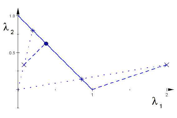
With the notation of Theorem 5.5, a non-orthogonal central projection equally well and uniquely determined has been proposed by Dryden et al. (2008) with
Orthogonal and central projection are depicted in Figure 1.
6 Local Effects of Curvature
In this section we assume that a manifold stratum supporting a random element is isometrically embedded in a Euclidean space of dimension . With the orthogonal projection from Section 3 and the Riemannian exponential of at we have the
respectively, of at , if existent.
6.1 Finite Power of Tests and Tangent Space Coordinates
With the above setup, assume that is a unique mean of . Moreover, we assume that is curved near , i.e. that there is , the center of the osculatory circle touching the geodesic segment in from to at with radius . If is the orthogonal projection of to that circle, then . Moreover, with
we have the residual tangent space coordinate
having squared length . By isometry of the embedding, the intrinsic tangent space coordinate is given by
With the component
of normal to the above mentioned geodesic segment of squared length , we obtain since
and . In consequence we have
Remark 6.1.
In approximation, the variation of intrinsic tangent space coordinates is the sum of the variation of residual tangent space coordinates and the variation normal to it. In particular, for spheres
Since the variation in normal space is irrelevant for a two-sample test for equality of means, say, a higher power for tests based on intrinsic means can be expected when solely residual tangent space coordinates obtained from an isometric embedding are used rather than intrinsic tangent space coordinates.
Note that the natural tangent space coordinates for Ziezold means are residual.
A simulated classification example in Section 7 illustrates this effect.
6.2 The - Property for Spherical and Kendall Shape Means
In this section is the -dimensional unit-hypersphere embedded isometrically in Euclidean -dimensional space. The orthogonal projection is well defined except for the origin , and the normal space at is spanned by itself. In consequence, a random point on has
as residual and intrinsic, resp., tangent space coordinate at where , .
Theorem 6.2.
If a.s. is contained in an open half sphere, it has a unique intrinsic mean which is assumed in the interior of that half sphere.
Proof.
Below, we show that every intrinsic mean necessarily lies within the interior of the half sphere. Then, (Kendall, 1990, Theorem 7.3) yields uniqueness. W.l.o.g. let such that and assume that is an intrinsic mean, . Moreover let . Since
with equality if and only if , this can only happen for . Now, suppose that is an intrinsic mean. For small deterministic consider . Then
with since . In consequence, cannot be an intrinsic mean. Hence, we have shown that every intrinsic mean is contained in the interior of the half sphere. ∎
Remark 6.3.
For the special case of spheres, this is a simple proof for the general theorem recently established by Afsari (2010) which extends results of Karcher (1977); Kendall (1990) and Le (2001); Le (2004), stating that the intrinsic mean on a general manifold is unique if among others the support of the distribution is contained in a geodesic half ball.
The following theorem characterizes the three spherical means.
Theorem 6.4.
Let be a random point on . Then is the unique extrinsic mean if and only if the Euclidean mean is non-zero. In that case
with . Moreover, there are suitable and such that every residual mean satisfies
and every intrinsic mean satisfies
In the last case we additionally require that which is in particular the case if is a.s. contained in an open half sphere.
Proof.
The assertions for the extrinsic mean are well known from Hendriks et al. (1996). The second assertion for residual means follows from minimization of
with respect to under the constraining condition . Using a Lagrange ansatz this leads to the necessary condition
with a Lagrange multiplier of value which is positive unless is supported by the hypersphere orthogonal to . In that case, by Proposition 3.3, cannot be a residual mean of , as every residual mean is as well contained in that hypersphere. Hence, we have .
The Lagrange method applied to
taking into account Theorem 6.2, insuring that is in the open half sphere that contatins a.s., yields the third assertion on the intrinsic mean. ∎
Recall that residual means are eigenvectors to the largest eigenvalue of the matrix . As such, they rather reflect the mode than the classical mean of a distribution:
Example 6.5.
Consider and a random variable on the unit circle which takes the value with probability and with probability . Then, explicit computation gives the unique intrinsic and extrinsic mean as well as the two residual means
Figure 2 shows the case .

In contrast to Figure 2, one may assume in many practical applications that the mutual distances of the unique intrinsic mean , the unique extrinsic mean and the unique residual mean closer to are rather small, namely of the same order as the squared proximity of the modulus of the Euclidean mean to , cf. Table 2. We will use the following condition
with the concentration parameter .
Corollary 6.6.
Proof.
Remark 6.7.
The tangent vector defining the great circle approximately connecting the three means is obtained from correcting with the expected normal component of any of the means. As numerical experiments show, this great circle is different from the first principal component geodesic as defined in Huckemann and Ziezold (2006).
Recall the following connection between top and quotient space means, cf. Theorem 4.5.
Remark 6.8.
Let such that a random shape on is supported by with at most countable. By Lemma 4.1 and Theorem 4.5, admits a horizontal measurable lift in optimal position to . Define the random variable on by . Then we have that
-
if is an intrinsic mean of then is an intrinsic mean of ,
-
if is a full Procrustean mean of then is a residual mean of ,
-
if is a Ziezold mean of then is an extrinsic mean of .
In consequence, Corollary 6.6 extends at once to Kendall’s shape spaces. Generalized geodesics referred to below are an extension of the concept of geodesics to non-manifold shape spaces, cf. Huckemann et al. (2010b).
Corollary 6.9.
Suppose that a random shape on with unique intrinsic mean , unique Ziezold mean and unique Procrustean mean is supported by . If the means are sufficiently close to each other in the sense of
with the random pre-shape on a horizontal lift of defined by , then the generalized geodesic segment between and is approximately divided by by the ratio with an error of order .
7 Examples: Exemplary Datasets and Simulations
All of the results of this section are based on datasets and simulations, i.e., all means considered are sample means. An R-package for the computation of all means including the poplar leaves data can be found under Huckemann (2010b).
7.1 The property
In the first example we illustrate Corollary 6.9 on the basis of four classical data sets:
- poplar leaves:
-
contains 104 quadrangular planar shapes extracted from poplar leaves in a joint collaboration with Institute for Forest Biometry and Informatics at the University of Göttingen, cf. Huckemann (2010b); Huckemann et al. (2010a).
- digits ’3’:
-
contains 30 planar shapes with 13 landmarks each, extracted from handwritten digits ’3’, cf. (Dryden and Mardia, 1998, p. 318).
- macaque skulls:
-
contains three-dimensional shapes with 7 landmarks each, of 18 macaque skulls, cf. (Dryden and Mardia, 1998, p. 16).
- iron age brooches:
-
contains 28 three-dimensional tetrahedral shapes of iron age brooches, cf. (Small, 1996, Section 3.5).


7.2 “Partial Blindness” of full Procrustes and Schoenberg Means
In the second example we illustrate an effect of “blindness to data” of full Procrustes means and Schoenberg means. The former blindness is due to the affinity of the Procrustes mean to the mode in conjunction with curvature, the latter is due to non-isometry of the Schoenberg embedding. While the former effect occurs only for some highly dispersed data when the analog of condition (6.2) is violated, the latter effect is local in nature and may occur for concentrated data as well.

Reenacting the situation of Section 4.4, cf. also Example 6.5 and Figure 2, the shapes of the triangles and in Figure 4 are almost maximally remote. Since the mode is assumed twice and only once, the full Procrustes mean is nearly blind to .


Even though Schoenberg means have been introduced to tackle 3D shapes, the effect of “blindness” can be well illustrated already for 2D. To this end consider , and as introduced in Remark 5.3. Along the horizontal geodesic through with initial velocity we pick two points and . On the orthogonal horizontal geodesic through with initial velocity pick . Recall from Remark 5.3, that along that geodesic the derivative of the Schoenberg embedding can be made arbitrarily small for near . Indeed, Figure 5 illustrates that in contrast to the intrinsic mean, the Schoenberg mean is “blind” to the strong collinearity of and .
7.3 Discrimination Power
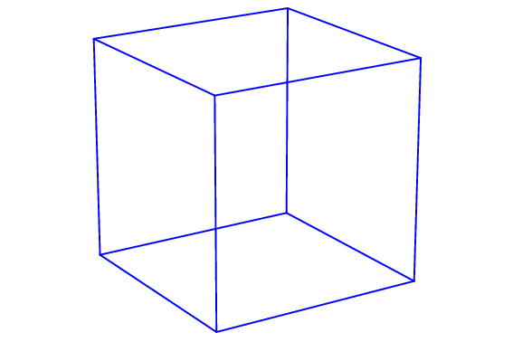
In the ultimate example we illustrate the consequences of the choice of tangent space coordinates and the effect of the tendency of the Schoenberg mean to increase dimension by a classification simulation. To this end we apply a Hotelling -test to discriminate the shapes of 10 noisy samples of regular unit cubes from the shapes of 10 noisy samples of pyramids with top section chopped off, each with 8 landmarks, given by the following configuration matrix
(cf. Figure 6) determined by . In the simulation, independent Gaussian noise is added to each landmark measurement. Table 3 gives the percentages of correct classifications.

As visible from Table 3, discriminating flattened pyramids () from cubes () is achieved much better by employing intrinsic or Ziezold means rather than Schoenberg means. This finding is in concord with Theorem 5.4: samples of size of two-dimensional configurations yield Euclidean means a.s. in which are projected to to obtain Schoenberg means in . In consequence, Schoenberg means of noisy nearly two-dimensional pyramids are essentially three dimensional. With increased height of the pyramid, (, i.e. for more pronounced third dimension and increased proximity to the unit cube) this effect waynes and all means perform equally well (or bad). Moreover in any case, intrinsic means with intrinsic tangent space coordinates qualify less for shape discrimination than intrinsic means with residual tangent space coordinates, cf. Remark 6.1. The latter (intrinsic means with residual tangent space coordinates) are better or equally well behaved as Ziezold means (which naturally use residual tangent space coordinates).
In conclusion we record the time for the computations of means in Table 4. While Ziezold means compute in approximately of the computational time for intrinsic means, Schoenberg means are obtained approximately times faster.
8 Discussion
By establishing stability results for intrinsic and Ziezold means on the manifold part of a shape space, a gap in asymptotic theory for general non-manifold shape spaces could be closed, now allowing for multi-sample tests of equality of intrinsic means and Ziezold means. A similar stability assertion in general is false for Procrustean means for low concentration. There is reason to believe, however, that it would be true for higher concentration. Note that the argument applied to intrinsic and Ziezold means fails for Procrustean means, since in contrast to the equations in Theorem 4.5 the sum of Procrustes residuals is in general non-zero. Loosely speaking, the findings on dimensionality condense to
- –
Procrustean means may decrease dimension by 2 or more,
- –
intrinsic and Ziezold means decrease dimension at most by 1, in particular, they preserve regularity,
- –
Schoenberg means tend to increase up to the maximal dimension possible.
Due to the proximity of Ziezold and intrinsic means on Kendall’s shape spaces in most practical applications, taking into account that the former are computationally easier accessable (optimally positioning and Euclidean averaging in every iteration step) than intrinsic means (optimally positioning and weighted averaging in every iteration step), Ziezold means can be preferred over intrinsic means. They may be even more preferred over intrinsic means, since Ziezold means naturally come with residual tangent space coordinates which may allow in case of intrinsic means for a higher finite power of tests than intrinsic tangent space coordinates.
Computationally much faster (not relying on iteration at all) are Schoenberg means which are available for Kendall’s reflection shape spaces. As a drawback, however, Schoenberg means, seem less sensitive for dimensionality of configurations considered than intrinsic or Ziezold means. In particular for problems involving small sample sizes and a large number of parameters as currently of high interest in statistcal applications, involving (nearly) degenerate data, Ziezold means may also be preferred over Schoenberg means due to higher power of tests.
Finally, note that Ziezold means may be defined for the shape spaces of planar curves introduced by Zahn and Roskies (1972), which are currently of interest e.g. Klassen et al. (2004) or Schmidt et al. (2006). Employing Ziezold means there, a computational advantage greater than found here can be expected since the computation of iterates of intrinsic means involves computations of geodesics which themselves can only be found iteratively.
Acknowledgment
The author would like to thank Alexander Lytchak for helpful advice on differential geometric issues.
Appendix A Proofs
Lemma A.1.
Let be a tubular neighborhood about that admits a slice via in optimal position to . Then, there is a measurable horizontal lift of in optimal position to .
Proof.
If is regular, then has the desired properties. Now assume that is not of maximal orbit type. W.l.o.g. assume that contains the closed ball of radius with bounding sphere and that there are having the distinct orbit types orccuring in . denotes all points on of orbit type , , respectively. Observe that each is a manifold on which acts isometrically. Hence for every , there is a finite () or countable () sequence of tubular neighborhoods covering , admitting trivial slices via
Here, denotes the Riemannian exponential of . Defining a disjoint sequence
exhausting we obtain a corresponding sequence of disjoint measurable sets with
Hence, setting
observe that every has a unique lift in which is contained in a unique . This lift is by construction (all are in ) in optimal position to . Moreover, if and for some with we have by the disjoint construction of and that , hence the isotropy groups of and agree, yielding . In consequence, is a measurable horizontal lift of in optimal position to . Since every horizontal geodesic segment , contained in features a constant isotropy group, except possibly for the initial point we obtain with the definition of
a measurable horizontal lift of in optimal position to . ∎
Proof of Theorem 4.4.
Since is connected, any two points can be brought into optimal position and a closed minimizing horizontal geodesic segment between can be found. If then also . In consequence, there are tubulars neighborhoods of and of admitting slices in optimal position to , which by Lemma A.1, have horizontal lifts and in optimal position to . Since is a manifold, there is a sequence , such that and that each is in optimal position to () and such that
with measurable horizontal lifts of . Defining and recursively for a measurable horizontal lift of in optimal position to is obtained. Finally, suppose that is in optimal position to for and set , if and () otherwise to obtain the desired measurable horizontal lift in optimal position to .
Proof of Theorem 4.7.
In case of intrinsic means, with the hypotheses and notations of the above proof of Theorem 4.4, suppose that is a measurable horizontal lift of in optimal position to an intrinsic mean of the random element on defined as in Theorem 4.5 with . For notational simplicity we assume that with a single tubular neighborhood of admitting a slice.
Then, additionally using the notation of the above proof of Lemma A.1, if the assertion of the Theorem would be false, w.l.o.g. there would be , , with and . In particular, in the proof Lemma A.1, we may choose a sufficiently small around such that in consequence of (8)
| (13) |
with some , and obtained from as in the proof of Lemma A.1. Suppose that is obtained as in the proof of Lemma A.1 by using and suppose that is obtained from by replacing the part of with . Then is also a measurable horizontal lift in optimal position to . Since we assume that is an intrinsic mean of , assertion (i) of Theorem 4.5 teaches that is also an intrinsic mean of lift of to , i.e.
This is a contradiction to (13) yielding the validity of the theorem for intrinsic means.
References
- Afsari (2010) Afsari, B., 2010. Riemannian center of mass: existence, uniqueness, and convexity. Proceedings of the American Mathematical Society 139, 655–773.
- Bandulasiri and Patrangenaru (2005) Bandulasiri, A., Patrangenaru, V., 2005. Algorithms for nonparametric inference on shape manifolds. Proc. of JSM 2005 Minneapolis, MN, 1617–1622.
- Bhattacharya (2008) Bhattacharya, A., 2008. Statistical analysis on manifolds: A nonparametric approach for inference on shape spaces. Sankhya, Ser. A 70 (2), 223–266.
- Bhattacharya and Patrangenaru (2003) Bhattacharya, R. N., Patrangenaru, V., 2003. Large sample theory of intrinsic and extrinsic sample means on manifolds I. Ann. Statist. 31 (1), 1–29.
- Bhattacharya and Patrangenaru (2005) Bhattacharya, R. N., Patrangenaru, V., 2005. Large sample theory of intrinsic and extrinsic sample means on manifolds II. Ann. Statist. 33 (3), 1225–1259.
- Bredon (1972) Bredon, G. E., 1972. Introduction to Compact Transformation Groups. Vol. 46 of Pure and Applied Mathematics. Academic Press.
- Choquet (1954) Choquet, G., 1954. Theory of capacities. Ann. Inst. Fourier 5, 131–295.
- Dryden et al. (2008) Dryden, I. L., Kume, A., Le, H., Wood, A. T. A., 2008. A multidimensional scaling approach to shape analysis. To appear.
- Dryden and Mardia (1998) Dryden, I. L., Mardia, K. V., 1998. Statistical Shape Analysis. Wiley, Chichester.
- Fréchet (1948) Fréchet, M., 1948. Les éléments aléatoires de nature quelconque dans un espace distancié. Ann. Inst. H. Poincaré 10 (4), 215–310.
- Gower (1975) Gower, J. C., 1975. Generalized Procrustes analysis. Psychometrika 40, 33–51.
- Hendriks and Landsman (1996) Hendriks, H., Landsman, Z., 1996. Asymptotic behaviour of sample mean location for manifolds. Statistics & Probability Letters 26, 169–178.
- Hendriks and Landsman (1998) Hendriks, H., Landsman, Z., 1998. Mean location and sample mean location on manifolds: asymptotics, tests, confidence regions. Journal of Multivariate Analysis 67, 227–243.
- Hendriks et al. (1996) Hendriks, H., Landsman, Z., Ruymgaart, F., 1996. Asymptotic behaviour of sample mean direction for spheres. Journal of Multivariate Analysis 59, 141–152.
- Huckemann (2010a) Huckemann, S., 2010a. Inference on 3D Procrustes means: Tree boles growth, rank-deficient diffusion tensors and perturbation models. Scand. J. Statist., to appear.
- Huckemann (2010b)
Huckemann, S., 2010b. R-package for intrinsic statistical analysis
of shapes,
http:www.mathematik.uni-kassel.de/huckeman/software/ishapes_1.0.tar.gz. - Huckemann et al. (2010a) Huckemann, S., Hotz, T., Munk, A., 2010a. Intrinsic MANOVA for Riemannian manifolds with an application to Kendall’s space of planar shapes. IEEE Transactions on Pattern Analysis and Machine Intelligence 32 (4), 593–603.
- Huckemann et al. (2010b) Huckemann, S., Hotz, T., Munk, A., 2010b. Intrinsic shape analysis: Geodesic principal component analysis for Riemannian manifolds modulo Lie group actions (with discussion). Statistica Sinica 20 (1), 1–100.
- Huckemann and Ziezold (2006) Huckemann, S., Ziezold, H., 2006. Principal component analysis for Riemannian manifolds with an application to triangular shape spaces. Adv. Appl. Prob. (SGSA) 38 (2), 299–319.
- Jupp (1988) Jupp, P. E., 1988. Residuals for directional data. J. Appl. Statist. 15 (2), 137–147.
- Karcher (1977) Karcher, H., 1977. Riemannian center of mass and mollifier smoothing. Communications on Pure and Applied Mathematics XXX, 509–541.
- Kendall (1974) Kendall, D., 1974. Foundations of a theory of random sets. Stochastic Geom., Tribute Memory Rollo Davidson, 322-376 (1974).
- Kendall et al. (1999) Kendall, D. G., Barden, D., Carne, T. K., Le, H., 1999. Shape and Shape Theory. Wiley, Chichester.
- Kendall (1990) Kendall, W. S., 1990. Probability, convexity, and harmonic maps with small image I: Uniqueness and fine existence. Proc. London Math. Soc. 61, 371–406.
- Klassen et al. (2004) Klassen, E., Srivastava, A., Mio, W., Joshi, S., Mar. 2004. Analysis on planar shapes using geodesic paths on shape spaces. IEEE Transactions on Pattern Analysis and Machine Intelligence 26 (3), 372–383.
- Kobayashi and Nomizu (1963) Kobayashi, S., Nomizu, K., 1963. Foundations of Differential Geometry. Vol. I. Wiley, Chichester.
- Kobayashi and Nomizu (1969) Kobayashi, S., Nomizu, K., 1969. Foundations of Differential Geometry. Vol. II. Wiley, Chichester.
- Krim and Yezzi (2006) Krim, H., Yezzi, A. J. J. E., 2006. Statistics and Analysis of Shapes. Modeling and Simulation in Science, Engineering and Technology. Birkhäuser, Boston.
- Le (2001) Le, H., 2001. Locating Fréchet means with an application to shape spaces. Adv. Appl. Prob. (SGSA) 33 (2), 324–338.
- Le (2004) Le, H., 2004. Estimation of Riemannian barycenters. LMS Journal of Computation and Mathematics 7, 193–200.
- Mardia and Patrangenaru (2001) Mardia, K., Patrangenaru, V., 2001. On affine and projective shape data analysis. Functional and Spatial Data Analysis, Proceedings of the 20th LASR Workshop (Eds: K.V. Mardia and R.G. Aykroyd), 39–45.
- Mardia and Patrangenaru (2005) Mardia, K., Patrangenaru, V., 2005. Directions and projective shapes. Ann. Statist. 33, 1666–1699.
- Matheron (1975) Matheron, G., 1975. Random sets and integral geometry. Wiley Series in Probability and Mathematical Statistics. New York.
- Nash (1956) Nash, J., 1956. The imbedding problem for Riemannian manifolds. Ann. of Math. 63, 20–63.
- Palais (1961) Palais, R. S., 1961. On the existence of slices for actions of non-compact Lie groups. Ann. Math. 2nd Ser. 73 (2), 295–323.
- Schmidt et al. (2006) Schmidt, F. R., Clausen, M., Cremers, D., 2006. Shape matching by variational computation of geodesics on a manifold. In: Pattern Recognition (Proc. DAGM). Vol. 4174 of LNCS. Springer, Berlin, Germany, pp. 142–151.
- Small (1996) Small, C. G., 1996. The Statistical Theory of Shape. Springer-Verlag, New York.
- Zahn and Roskies (1972) Zahn, C., Roskies, R., 1972. Fourier descriptors for plane closed curves. IEEE Trans. Computers C-21, 269–281.
- Ziezold (1977) Ziezold, H., 1977. Expected figures and a strong law of large numbers for random elements in quasi-metric spaces. Trans. 7th Prague Conf. Inf. Theory, Stat. Dec. Func., Random Processes A, 591–602.
- Ziezold (1994) Ziezold, H., 1994. Mean figures and mean shapes applied to biological figure and shape distributions in the plane. Biom. J. (36), 491–510.