Collider Phenomenology with Split-UED
Abstract:
We investigate the collider implications of Split Universal Extra Dimensions. The non-vanishing fermion mass in the bulk, which is consistent with the KK-parity, largely modifies the phenomenology of Minimal Universal Exta Dimensions. We scrutinize the behavior of couplings and study the discovery reach of the Tevatron and the LHC for level-2 Kaluza-Klein modes in the dilepton channel, which would indicates the presence of the extra dimensions. Observation of large event rates for dilepton resonances can result from a nontrivial fermion mass profile along the extra dimensions, which, in turn, may corroborate extra dimensional explanation for the observation of the positron excess in cosmic rays.
Keywords:
Beyond Standard Model, Extra Dimension, Kaluza-Klein particle1 Introduction
Models with extra spatial dimensions allow us to confront some of the outstanding issues of the Standard Model (SM) (see [1, 2, 3]). In particular, the Universal Extra Dimensions (UED) scenario [4] leads to an interesting dark matter candidate [5, 6, 7, 8, 9] as well as a foil for searches for Supersymmetry at colliders [13, 12, 10, 11]. In the original minimal UED picture (MUED), all of the SM fields live in a 5-dimensional orbifolded bulk with a compactification radius . Due to the breaking of 5D Lorentz invariance, Kaluza-Klein (KK) number is no longer conserved although a symmetry, KK-parity, remains. This being the case, the tree-level wave functions for the various KK states are either sines or cosines in the coordinate of the extra dimension. Allowing for radiative loop corrections to the tree-level particle masses, the physics of MUED is then described by only two parameters beyond those of the SM [14]: and a cutoff scale, , used to define these loop corrections, which is usually taken such that but with only logarithmic sensitivity to this particular choice.
In MUED and its extension to higher dimensions [15, 16, 17, 18], the bulk masses of the SM fermions are taken to be zero. However, this is no longer the case in Split-UED (SUED) [19, 20, 21, 22]. Indeed this ‘bulk mass’ term is naturally included in the effective Lagrangian as the term is compatible with 5D Lorentz invariance as well as gauge invariance of the model. Here one notes that in order to maintain the KK parity the ‘coefficient’ of the fermion bilinear term in the action must be an odd function of the 5D coordinate, , defined on an interval, where . The simplest choice to make in this case, as is similarly done in the Randall-Sundrum (RS) model, is to write this coefficient as , where is a dimensionful parameter whose value is, in general, dependent upon which SM field is being considered and for . Naturally, one might expect that the values of can be of either sign and be of order . The effects of including a non-zero value for are two-fold: First, depending upon its sign, the fermion zero-modes, which are identified with the known SM fermions, no longer have flat wave functions in the extra dimension. These are now found to be either peaked near or at the orbifold boundaries; this leads to potentially large differences in the various couplings of these fermions to the KK gauge fields from those expected in MUED. In particular, the zero mode fermions now have tree-level couplings to the KK-number even gauge modes. Second, the KK fermion wave functions and masses (which are given by at tree-level) are now somewhat more complicated and are explicitly dependent upon the specific value of the parameter. In particular, the expressions for the KK fermion masses are different depending upon whether the relevant KK-number is even or odd.
The purpose of this paper is () to explore in some of the detailed implications of non-zero values for fermion mass parameter leading to alterations from the conventional MUED phenomenology and () to investigate the regions in the plane which are accessible to current and future collider experiments. To these ends, in Section 2, we provide a basic overview of the masses, wave functions and couplings of the fermion KK states in split-UED model and display their explicit dependence upon the parameter pointing out important differences with the MUED case. Here we will assume that the parameter takes on a universal value for all fermions for simplicity of the analysis so that there is only one new parameter to consider beyond that of MUED. In Section 3 we will discuss the collider phenomenology of split-UED and, in particular, the properties of the KK states and the potential for their discovery at the LHC. Further, we obtain the regions of the plane which are allowed by current experimental data and show the regions which will be made accessible by searches at the LHC. Our conclusions can be found in Section 4. Appendix A contains detailed information of KK decomposition and mass spectrum.
2 Split Universal Extra Dimensions
2.1 Model
Universal extra dimensions postulates that all of the Standard Model particles are propagating in a small extra dimension(s). Orbifold compactification makes it possible to construct a chiral four dimensional effective theory. In contrast to the brane world scenarios [1, 2], the translational symmetry along the extra dimension leads to a remnant discrete symmetry, dubbed KK parity, so that the lightest Kaluza-Klein particle can be a good dark matter candidate. Also this parity mimics the R-parity in supersymmetric theory so that UED phenomenology shares several common features with MSSM [12]. On the other hand, it has been often overlooked in UED models that the bulk Dirac masses are generically allowed and are not in conflict with higher dimensional Lorentz symmetry or gauge invariance. In this section, we review split-UED model where these bulk Dirac masses are generically allowed in a way that KK parity is intact.
In split-UED, quarks and leptons are all promoted to fields in five dimensional spacetime on orbifold with two fixed points and , respectively, where is the coordinate along extra dimension with the half length . In the minimal setup, the gauge group is the same as in the Standard Model: under which charges are assigned as follows
| (1) |
where the index runs for three generations of fermions. Allowing bulk mass term in split-UED the generic action is given by
| (2) |
where the covariant derivative is with the usual Gell-Mann and Pauli matrices and . The , , and , , are the gauge coupling constants and the gauge fields of the corresponding gauge groups, respectively. Without loss of generality we can diagonalize the action in Eq. (2) by unitary transformations. Therefore the mass term can be taken as and there is no kinetic mixing between different flavors (for ). In general, we may have dimensionful parameters for each generation. Now imposing Dirichlet boundary conditions for unnecessary chiral component of fermions, we can finally get exactly the same spectra in the SM for the lowest Kaluza-Klein modes. All the details of derivation to get the Kaluza-Klein spectra are described in the Appendix. The most prominent feature of split-UED is that the fermion profile in the extra dimension is either localized near the origin or at boundaries depending the sign of bulk mass parameter in a way that Kaluza-Klein parity is respected. Having a non-zero bulk mass, , a field still has a massless zero mode which satisfies Neumann boundary conditions. However its Kaluza-Klein excitation states get additional contributions and the mass is given by where is the momentum to the extra dimension which is determined by for or for . Here we impose Dirichlet boundary conditions for modes so that contains the SM fermions in our convention. We assume that gauge sector and Higgs sector remain the same as in the conventional UED models. Therefore the zero modes have flat profiles and Kaluza-Klein modes have cosine wave functions satisfying Neumann boundary conditions.
In summary, in split-UED, there are new dimensionful parameters for three generations, the cutoff scale () and one length parameter () given by the size of extra dimension in addition to the SM parameters. In this study we will consider all bulk mass parameters are the same for simplicity, and study region 11 1 For , the KK spectra contain the unacceptable light modes below KK scale TeV..
2.2 Behavior of couplings
Having the explicit wave functions of fields as given in the Appendix, we can calculate the explicit Lagrangian for interactions among those fields. Essentially the overlap integral of the wave functions gives the effective couplings. For a gauge boson after choosing a simplifying gauge to get rid of the fifth component of gauge multiplet, , by the orbifold condition, we find
| (3) | |||||
| (4) | |||||
| (5) |
where the effective coupling is obtained by the integration of the wave function overlap with a convenient dimensionless variable :
| (7) | |||||
As the profiles of gauge bosons are universal and the profile of fermions depend on the bulk mass parameter , the overlap integral is the same for all gauge bosons but depends on . The suppressed gauge group indices should be understood.
Let us now see the coupling between KK bosons () of , and and the zero mode SM fermion pair for the definiteness 22 2 As it is clear in minimal UED, the weak mixing angles for KK gauge bosons are suppressed by . Thus essentially gauge eigenstates are well aligned by mass eigenstates.. The zero mode wave function profile for SM fermion is given by
| (8) |
If , the profile is exponentially localized near the center (at the boundaries). The zero mode is massless in the absence of the electroweak symmetry breaking even though its KK modes get additional mass from the bulk mass .


The KK gauge bosons commonly have the same profiles as in MUED
| (9) |
and the zero mode profile, , is flat, as shown in Fig. 1. Note that . The coupling of level- bosons to SM fermion pair is now written as
| (10) |
where is a dimensionless parameter measuring the overlap of wave functions between two SM fermions and a KK gauge boson defined as
| (11) | |||||
where and is explicitly calculated to be
| (15) |
From the KK-parity conservation, is easily understood. The Standard Model coupling constants are obtained as
| (16) |
as independent of . Here denotes the effective coupling constant for the interaction. Finally for the even ’s we get the coupling between the Standard Model fermions and even-KK excitation states of gauge bosons, as
| (17) |


The various couplings associated with one vector boson and two fermions are shown in Fig. 2. We find that there are two interesting regions. One is the MUED limit, i.e., , which is shown as the vertical solid line (in magenta) and the other is large positive limit. For , the zero mode fermions are well localized near the center () so that their couplings to KK gauge bosons asymptotically approach to the well known value as one can see the red curve for (Fig. 2(a)) as well as the curves for (Fig. 2(b)). The alternating sign can be understood as the -th KK gauge boson wave function in Eq. (9) is proportional to at where the fermion wave function is mostly localized. The is from the zero mode normalization in Eq. (16). These vertices are all vanishing in the limit of because of KK number conservation in MUED.
For collider phenomenology, we are mostly interested in interactions for low lying Kaluza-Klein modes, as heavier modes are too massive and easily decouple from the low energy phenomenology. The most relevant couplings in our study are the interactions and decays of the second Kaluza-Klein gauge boson.
The coupling -- remains the same for all due to the normalization condition of wave functions for -th fermion profile, while all other couplings now change for non-vanishing bulk masses. The -- coupling remains zero in SUED but in principle this coupling can be generated by the unknown physics at the cutoff scale (), and the lowest order coupling may take the form [14]
| (18) |
However, being higher dimensional, we expect it to be suppressed at least by one power of , hence we shall neglect it in the discussion that follows.
It is interesting to notice that the coupling for the KK gluon can be chiral. Let us examine the level- gluon couplings with quarks:
| (19) |
All the KK-parity violating interactions are forbidden. Now it is obvious that KK-gluon has chiral interactions with the SM quarks, if or , in general. Finally the vector (V) and axial-vector (A) couplings of KK gluons with an up-type quark and a down-type quark,
| (20) |
are determined as
| (21) | |||
| (22) |
The same is similarly true for all other gauge bosons as well. When , only the vectorial coupling is non-vanishing. However, in general, and the non-vanishing axial couplings are allowed. For instance, if and , the vectorial and axial couplings have opposite signs but have the same size: . With non-vanishing axial couplings in the even KK gauge boson interactions, one might expect, for instance, additional contribution to the forward-backward asymmetry of the top quark pair production () via the quark pair annihilation channel. The cross-section for annihilation into top quarks of mass through the -th KK gluons reads
| (23) | |||||
where is the polar angle of the top quark with respect to the incoming quark in the center of mass rest frame, is the squared partonic invariant mass, is the velocity of the top quark, with . The parameters and represent, respectively, the vector and axial-vector couplings of the KK gluons to the light quarks (top quarks).
Considering experiments at Tevatron, the parton level energy is typically much less than the KK gluon mass so that the interference term (the second term) is dominant over the pure new physics term (the third term). And the leading contribution in the second term is the interference between two diagrams the SM gluon and the level-2 KK gluon. As the tree level SM contribution (the first term) does not produce the forward-backward asymmetry after integrating over , the main contribution is from the linear term of cosine in the second term for :
| (24) |
When , and ,
| (25) |
thus the forward-backward asymmetry is positive, which is consistent with the recent measurements at Tevatron [23, 24, 25], but we find that its size is not large enough to explain the current anomaly for TeV.
2.3 Mass spectrum
The mass spectrum of fermions gets tree level modifications from the bulk parameters as well as the loop induced mass correction from the RG running effect for a given boundary condition at some high scale just as in the case in conventional UED. Taking the vanishing boundary condition at , it is known that the one-loop induced mass correction is minor ( level for electroweak particles). This is due to lack of long RG running from which is argued to be less than TeV based on naive dimensional analysis (see e.g. [26]). Thus we may neglect the loop-induced mass correction for fermions as long as the bulk mass parameter is sufficiently large .
The mass of KK fermon () gets contributions from the bulk mass at tree level as follows
| (26) |
where
| (27) | |||
| (28) |
In the MUED limit, , Eqs. (27-28) both reduce to . On the other hand, all KK boson masses remain the same, , and show no dependence.
Including EW symmetry breaking and the radiative corrections, a naive estimate gives
| (29) | |||||
| (30) |
where is expected from the electroweak symmetry breaking.
2.4 Constraints from contact interactions
One of the most prominent features of SUED having non-vanishing bulk mass parameters is the existence of tree level KK number violating interactions. From exchange diagrams we can effectively obtain the contact interaction Lagrangian which is stringently constrained by electroweak precision measurements [27, 28]
| (31) |
u d (TeV) 10.2 6.0 12.5 8.6 (TeV) 8.3 4.3 11.9 8.2
.
Assuming a universal bulk mass , the and mediated interaction effective Lagrangian is obtained. The most stringent bound comes from the contact interaction for :
| (32) |
Taking Eqs. (31-32) into account with , we obtain the following relations:
| (33) | |||||
| (34) |
where the bounds for and are given in Table 1.
We also consider the constraints arising from the dilepton resonance searches at Tevatron [29] and find that those for give a slightly better constraint on than those for , while gives a similar limit to that for [30]. In the next Section we include these as well as constraints from contact interactions.
3 Collider phenomenology
A large amount of effort has given into examining the collider aspects of Universal Extra Dimensions [4] at LHC [13, 12, 10, 15, 16] and ILC [11, 17], as well as its astrophysical implications [5, 6, 7, 8, 18, 9]. In this Section we would like to investigate the implications of non-vanishing bulk mass in SUED.
3.1 Level-1 modes
We start our discussion with the level-1 KK modes. Their phenomenology depends on the precise value of the bulk mass and the radiative corrections to KK masses. Therefore here we would like discuss only generic features.
A small value for the bulk mass () would give the similar decay patterns as in the MUED case. The dominant production is provided by the strong interaction at a hadron collider, i.e., KK quark production (, and ), KK gluon production () and associated production (, ). The -doublet KK quarks () dominantly decay into KK gauge bosons ( and ) while the -singlet KK quarks () decay into KK photon. SM leptons are obtained from the decay of EW gauge bosons ( and ) to KK leptons. Here the difference with MUED would be the mass splitting between each mode. A bulk mass term would increase the mass of the KK fermion, making the decay product of KK bosons softer than that in MUED. However the other decay products from the KK fermions to KK bosons become more energetic due to the increased splitting. For instance, KK quarks can have mass just below the KK gluon and the jet from the decay of KK gluon () would be softer while the jet from the decay of KK quark ( or ) becomes harder than in MUED. The same is true for KK leptons and KK gauge bosons. However we do not expect a dramatic change in the reach for this model, as long as the decay patterns are the same and the mass splitting is not too small.
The other extreme limit is the case of very large , 33 3 The opposite limit (a large negative ) is also interesting as shown in the Appendix. In this case, taking a very large , the masses of the level-1 KK fermions remain at EW scale while all other KK fermions at higher level are decoupled from the theory due to the large mass splitting between the level-1 and the level-2 KK fermions. All KK bosons are also very heavy due to the large . Therefore in this limit, the only available KK modes are the level-1 KK leptons and quarks. This study will be elsewhere [31].. In this case, all KK fermions become much heavier than KK bosons and they may not be within the reach of the LHC. KK gauge bosons go through 3 body decays to the KK photon ( and ) and production would be via the KK gluon () and EW gauge bosons () 44 4 , and involve KK fermions in the - and -channels and their production cross sections are negligible for heavy KK quarks.. It is interesting to notice that this situation is similar to the focus point region of supersymmetry.
For the moderate ranges of the bulk mass (), the gauge bosons may still go through 3-body decays while the LHC will be able to produce KK quarks and KK leptons. Unlike MUED, now all KK quarks dominantly decay to the KK gluon since it has the largest coupling. Therefore the collider signature would be quite jetty.
An interesting possibility is that all KK fermions are very heavy with a large so that they are unobservable but still the KK bosons are within the reach of the LHC. Even in this case, we might expect to observe e.g. the level-2 gluon through its interaction with the level zero Standard Model quarks with a sizable coupling (). Dilepton production through and is also sizable and provides a golden search channel for split-UED. Detection of a dark matter (DM) particle, on the other hand, is quite challenging because the DM-SM coupling through the level-1 fermion will be highly suppressed by the large KK fermion mass.
We plot cross sections for the gauge boson production at the LHC, as function of mass in Fig. 3, assuming ; here the curve is dotted for (in black), solid for (in red) and dashed for (in blue). For KK gluon pair production from the initial state, there are -, -, - and four point interaction diagrams, and all couplings are fixed by gauge invariance. There is a contribution from the initial state but it is smaller than that from at the LHC for the mass range shown. is produced by exchange in the -channel and contribution from KK quarks in the - and -channels. Having these 3 diagrams is also necessary by gauge invariance and neglecting any of them gives inconsistent results. However in our case, considering the limit where the KK quarks are much heavier than KK gauge bosons, their exchanges with a few TeV in mass barely affects the production cross sections.

From Fig. 2 we can immediately read off the patterns of KK particle decay branching fractions. The level-1 gauge boson only couples to thanks to KK parity. This coupling becomes less significant as becomes larger in which case the level-1 fermion becomes significantly heavier than the level-1 gauge boson. Due to the large mass gap, the decay products of the level-1 fermion are reasonably energetic.
3.2 Level-2 modes
Now we turn to discussion of the level-2 KK modes. In general level-2 KK fermions () can decay into either two level-1 KK states or one level-2 and one SM mode (the branching fraction of to is suppressed by the small mass splitting between and .). In the limit of in split-UED, all KK fermions masses are raised, and level-2 KK quarks ( and ) decay to and . Then gives rise to a missing energy signature through a 3 body decay while can directly decay into two jets and may appear as dijet resonance.
In MUED, the coupling of level-2 resonances to the SM fermions is suppressed by 1-loop. The branching fractions of electroweak level-2 gauge bosons into dilepton final states are small partly due to the competing decay modes into other level-2 and level-1 KK states, and partly due to difference between the strong and electroweak couplings. Therefore one has to rely on indirect production of level-2 KK gauge bosons from the KK gluon and KK quarks to enhance the production cross sections. The corresponding reach has been estimated in Ref. [10].
In SUED, however, this coupling exists at tree level due to the fermion bulk mass term and it could be as large as times the corresponding SM coupling strength, which makes dilepton searches in this model promising. At the same time, the bulk mass increases the mass of KK fermions, thus reducing the branching fraction of level-2 bosons into other KK states. The decay width of level-2 KK bosons into SM fermion final states is given by
| (35) | |||||
| (36) |


The 1-loop correction is expected to be the smallest for among all other KK states at the same level, and in fact, KK photons receive negligible correction from RG running, making the lightest KK photon a viable dark matter candidate. Therefore the decay channels of into - or - are closed and always can appear as a resonance. As in Eqs. (35)-(36), the width dependence on the SM fermion mass is negligible even for the top quark, if the resonance is heavy enough. In this case, the ratio of the total width to its mass becomes mass-independent. The total width of () is then 7% (3.5%) of its mass as increases, as shown in Fig. 4(a), while in MUED, the widths of level-2 KK bosons are much less than 1% [10]. This makes it challenging to probe double resonances which are separated from each other in mass by the small 1-loop corrections (7% or so).
The branching fractions of the are -independent for a universal bulk mass, which is the case that we consider. They are 25% in dilepton, 36.7% in dijet, 4.2 in , 14% and 12.5% in . The decays invisible through SM neutrinos 7.5% of the time. Notice that the branching fraction into dilepton channel is about 20 times larger than in case of MUED.
The decay of is somewhat more complicated than due to the slightly larger 1-loop correction, which we assume to be about 7% as in the MUED. In this case the decay modes to other KK states remain open. Without knowing the exact 1-loop mass corrections for all KK particles, it is impossible to compute its total width and branching fractions. For a rough estimate (only for this purpose), we assume that KK fermions only gets corrections from the bulk mass while gets heavier by 7% from RG running. This is certainly an inconsistent setup. However, 1-loop corrections to KK fermion masses are known to be merely a few percents (1% for singlet KK fermions and 3% for doublet KK fermions), and for a large , bulk mass enhances its mass by quite a large amount and this 1-loop contribution becomes negligible. This approximation is valid in a broad range of . Given that, one can compute the partial widths of in three different channels and the results are shown in Fig. 4(b). The level-2 KK fermion does not get correction from the bulk mass, but the -- coupling becomes smaller, as shown in Fig. 2, making the relevant branching fraction smaller for large . The same is true for -- while -- coupling behaves in the opposite manner. Moreover, unlike , the level-1 KK modes get heavier as the increases, and at some value of , the decay to gets closed. In Fig. 4(b), this transition value of is about 0.6 for a 1 TeV .
Having -- as a dominant channel, it is straightforward to compute the relevant branching fractions. Since () couples to SM pair with the same strength, one needs to count relevant degrees of freedom. The branching fractions are 1/24 in , 1/12 in dilepton, 1/2 in dijet and 1/8 in either and . also can decay invisibly 1/24 of the time.
3.3 The LHC reach for and in dilepton channel
We simulate dilepton resonances in the Split-UED at the LHC with =10 TeV, using a private Monte-Carlo generator. We assume the mass splitting between two bosons ( and ) is given by and as in MUED. We include both and in the dilepton signal and use the CTEQ6.6 PDF with NLO K-factor. The leptons from the decay of these KK bosons are highly energetic and can easily pass triggers. For heavy resonances, the energy resolution is better in electron final states than in muon final states, and hence we consider electron final state with 1% mass resolution smearing. and GeV are imposed as cuts and we only count events with dielectron masses greater than 0.8 of . The dominant background is Drell-Yan, and and fakes are expected to be significantly smaller. In all cases the background is smaller than the signal by a factor of 100.
Fig. 5(a) shows the required luminosity to observe at least 10 signal events as a function of for several values of masses. The LHC should able to cover the large parameter space (up to TeV for ) even with the early data at the level of 100 pb-1 or less. With the integrated luminosity of 100 fb-1, the most of parameter space would be probed, setting limit on the bulk mass and the mass of the KK gauge boson.
The expected number of signal events is plotted in the versus plane in Fig. 5(b), for fb-1. The shaded region in the left side (in yellow) is a projected Tevatron exclusion at 95% C.L. assuming 10 fb-1 [29]. The limit on from gives the best exclusion since it is lighter than and by 7%, and constrains on and are comparable, and hidden below that from . The other shaded area in the left upper corner (in green) is EW constraint from LEP II considering contact interaction in SUED, as discussed in Section 2.4.


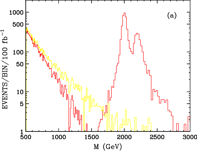
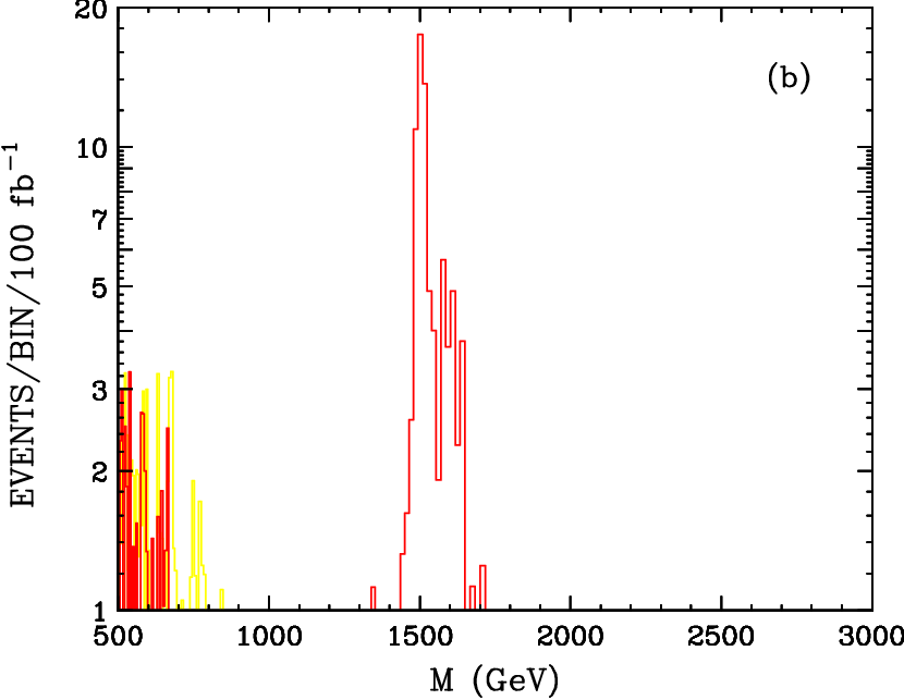
In Fig. 6 invariant mass distributions are shown for (a) TeV, TeV and fb-1 and (b) TeV, TeV and fb-1. For both cases, we assume . The yellow histogram is the SM background while the red histogram includes both signal and backgrounds. At the early phase of LHC, one may able to see a bump and get to resolve it into double resonance structure as more data gets accumulated. Notice the negative interference between the SM background and the KK signal, which implies the relative sign difference in the couplings.
4 Conclusions
The Minimal Universal Extra Dimensions scenario has received great attention. Recently non-vanishing bulk fermion masses have been introduced without spoiling the virtue of KK-parity. The fermion profiles are no longer simple sine/cosine functions and depend upon the specific values of bulk parameters. The profiles of fermions are split along the extra dimensions while the wave functions of the bosons remain the same as in UED. A simple introduction of a KK-parity conserving bulk fermion mass has significant influences on collider aspects as well as astrophysical implications of UED. For instance, the DM annihilation fraction into certain SM fermion pairs is either enhanced or reduced (compared to the MUED case) so that one can perhaps explain the PAMELA positron excess while suppressing the anti-proton flux.
In this paper, we have concentrated on collider phenomenology of Split Universal Extra Dimensions. We have revisited the KK decomposition in detail and analyzed wave function overlaps to compute relevant couplings for collider studies. We have discussed general collider implication for level-1 KK modes and level-2 KK with non-zero bulk mass and have computed LHC reach for the EW level-2 KK bosons, and , in the dilepton channel. The LHC should able to cover the large parameter space (up to TeV for ) even with early data assuming 100 pb-1 or less.
The existence of double resonances is one essential feature arising from extra dimensional models. Whether or not one can see double resonances depends both on how degenerate the two resonances are and on the mass resolution of the detector. The very high from the decay makes resolution in dimuon channel worse than in dielectron final state. This is because one can reconstruct electron from ECAL but muon momentum reconstruction relies on its track, which is barely curved in this case. Further indication for SUED might be the discovery of -like signature of mass close to . The MUED predicts a somewhat lower event rate due to 1-loop suppressed coupling of level-2 bosons to SM fermion pair, while it exists at tree level in SUED. Therefore in UED, one has to rely on indirect production of level-2 bosons, whose collider study requires complete knowledge of the model: the mass spectrum and all the couplings. On the other hand, in the large limit of SUED, the dependence on mass spectrum is diminished since level-2 KK bosons decay only into SM fermion pairs. This allows us to estimate the signal rate from their direct production, so that they can be discovered at the early phase of the LHC. The indirect production mechanism only increases production cross sections, improving our results.
Once a discovery has been made, one should try to reconstruct events and do further measurements such as spin and coupling determination, with more accumulated data [32, 33, 34], which might discriminate KK resonances from other models. The coupling measurement is directly related to the determination of the bulk masses. A challenging issue might be the existence of two resonances which are rather close to each other.
Acknowledgments.
We thank J. Shu and K. Wang for discussion on the forward-backward asymmetry and also thank C. Csáki, J. Heinonen and J. Hubisz for helpful discussion. S. Park is supported by the World Premier International Research Center Initiative (WPI initiative) by MEXT and also supported by the Grant-in-Aid for scientific research (Young Scientists (B) 21740172) from JSPS, Japan. K. Kong and T. G. Rizzo are supported in part by the DOE under contract DE-AC02-76SF00515.Appendix A Appendix: Fermion spectrum in split-UED
Let us consider a massive fermion on an orbifold with the radius of the circle . Two fixed points are at and where . The action is
| (A.1) |
where the gamma matrices in 5D are .
A Dirac mass is allowed in general. To keep KK-parity, the bulk mass must be odd under inversion . We can choose the simplest kink type mass
| (A.2) |
where and . The left (right)-chiral fermion is defined as usual and a generic Dirac fermion is decomposed as . Then the action is
| (A.3) | |||||
Varying the action with respect to and we obtain the standard bulk equations of motion which are given by
| (A.4) | |||||
| (A.5) |
then using we finally obtain
| (A.6) |
A.1 KK decomposition and wave equations
Now we would like to discuss how to perform the Kaluza–Klein decomposition of these fields. In general, when the fermion belongs to a complex representation of the symmetry group, the KK modes can only acquire Dirac masses and the KK decomposition is of the form
| (A.7) |
where are 4D spinors which satisfy the Dirac equations:
| (A.8) |
Plugging this expansion into the bulk equations we obtain the following set of coupled first order differential equations for the wave functions :
| (A.9) |
Applying on the first order equations we find a decoupled second order equations in the bulk:
| (A.10) | |||||
where , where means .
A.2 Zero mode solution:
For , we can find a massless solution () rather easily. In the bulk (), Eq. (A.9) is reduced to simple first order equations:
| (A.11) |
having the simple solutions
| (A.12) |
where the normalization factors are obtained from the condition :
| (A.13) |
Depending on the sign of the shapes of wave functions are determined. If , e.g., is localized near the middle point () and towards the end points ().
A.3 KK mode solution: Heavy modes ()
Depending on the sign of the wave functions will be either sines and cosines or hyperbolic sines and hyperbolic cosines. Here we first consider the case with . In this case the KK modes are heavier than the bulk mass since . We call them the heavy modes.
The wave equation for the heavy modes looks simple as:
| (A.14) |
and their generic solutions are
| (A.15) |
If ’s are zero, and thus the Dirichlet boundary conditions are reduced to a simple relation:
| (A.16) |
This equation determines the spectrum of even excitation modes.
If ’s are non-zero, on the other hand, we get a different set of master equation for Kaluza-Klein spectrum. First, ’s and ’s are related by Eq. (A.9):
| (A.17) | |||
| (A.18) |
From the continuity condition at the origin () we get a useful formula:
| (A.19) |
where we have used from the continuity condition.
Now let us consider boundary conditions. We can have two independent choices of Dirichlet boundary conditions according to the orbifold condition: (DL) or (DR).
| (A.20) | |||||
| (A.21) |
or
| (A.22) |
Now combining the continuity condition in Eq. (A.19) and the Dirichlet boundary condition in Eq. (A.22) we get the master equation:
| (A.23) |
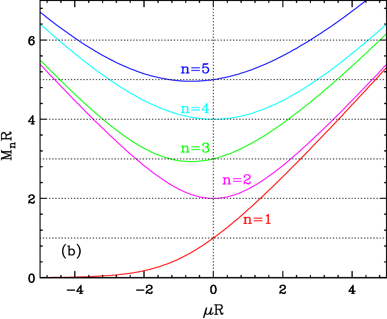
This equation determines the KK spectrum for odd excitation modes for any given value of (See Fig. 7(a) and 7(b) for DL and DR, respectively).


A.4 KK mode solution: Light mode ()
Here we first consider the case with . In this case the KK modes are lighter than the bulk mass since . We call them the light modes.
The wave equation for the light modes looks simple:
| (A.24) |
and their generic solutions are
| (A.25) |
’s and ’s are related by Eq. (A.9):
| (A.26) | |||
| (A.27) |
From the continuity condition at the origin () we get a useful formula:
| (A.28) |
where we have again used from the continuity condition.
Now let us consider boundary conditions. As before we can have two independent choices of Dirichlet boundary conditions according to the orbifold condition: (DL) or (DR).
| (A.29) | |||||
| (A.30) |
or
| (A.31) |
Now combining the continuity condition in Eq. (A.28) and the Dirichlet boundary condition in Eq. (A.31) we get the master equation:
| (A.32) |
for (DL/DR), respectively. This equation determines the KK spectrum for light modes. In contrast to the heavy modes, light modes can exist only for certain range of . For (DL/DR), a solution can exist only when , respectively (See Fig.8). For instance, if , a light mode solution is not allowed for (DL). In this case a zero mode, , is localized near the center (). On the other hand, if , a light mode solution is not allowed for (DR) and the zero mode, , is localized toward the center.

References
- [1] N. Arkani-Hamed, S. Dimopoulos and G. R. Dvali, “The hierarchy problem and new dimensions at a millimeter,” Phys. Lett. B 429, 263 (1998) [arXiv:hep-ph/9803315].
- [2] L. Randall and R. Sundrum, “A large mass hierarchy from a small extra dimension,” Phys. Rev. Lett. 83, 3370 (1999) [arXiv:hep-ph/9905221].
- [3] H. Davoudiasl, S. Gopalakrishna, E. Ponton and J. Santiago, “Warped 5-Dimensional Models: Phenomenological Status and Experimental Prospects,” arXiv:0908.1968 [hep-ph].
- [4] T. Appelquist, H. C. Cheng and B. A. Dobrescu, “Bounds on universal extra dimensions,” Phys. Rev. D 64, 035002 (2001) [arXiv:hep-ph/0012100].
- [5] G. Servant and T. M. Tait, “Is the lightest Kaluza-Klein particle a viable dark matter candidate?,” Nucl. Phys. B 650, 391 (2003) [arXiv:hep-ph/0206071].
- [6] H. C. Cheng, J. L. Feng and K. T. Matchev, “Kaluza-Klein dark matter,” Phys. Rev. Lett. 89, 211301 (2002) [arXiv:hep-ph/0207125].
- [7] K. Kong and K. T. Matchev, “Precise calculation of the relic density of Kaluza-Klein dark matter in universal extra dimensions,” JHEP 0601, 038 (2006) [arXiv:hep-ph/0509119].
- [8] F. Burnell and G. D. Kribs, “The abundance of Kaluza-Klein dark matter with coannihilation,” Phys. Rev. D 73, 015001 (2006) [arXiv:hep-ph/0509118].
- [9] S. Arrenberg, L. Baudis, K. Kong, K. T. Matchev and J. Yoo, “Kaluza-Klein Dark Matter: Direct Detection vis-a-vis LHC,” Phys. Rev. D 78, 056002 (2008) [arXiv:0805.4210 [hep-ph]].
- [10] A. Datta, K. Kong and K. T. Matchev, “Discrimination of supersymmetry and universal extra dimensions at hadron colliders,” Phys. Rev. D 72, 096006 (2005) [Erratum-ibid. D 72, 119901 (2005)] [arXiv:hep-ph/0509246].
- [11] M. Battaglia, A. Datta, A. De Roeck, K. Kong and K. T. Matchev, “Contrasting supersymmetry and universal extra dimensions at the CLIC multi-TeV e+ e- collider,” JHEP 0507, 033 (2005) [arXiv:hep-ph/0502041].
- [12] H. C. Cheng, K. T. Matchev and M. Schmaltz, “Bosonic supersymmetry? Getting fooled at the LHC,” Phys. Rev. D 66, 056006 (2002) [arXiv:hep-ph/0205314].
- [13] T. G. Rizzo, “Probes of universal extra dimensions at colliders,” Phys. Rev. D 64, 095010 (2001) [arXiv:hep-ph/0106336].
- [14] H. C. Cheng, K. T. Matchev and M. Schmaltz, “Radiative corrections to Kaluza-Klein masses,” Phys. Rev. D 66, 036005 (2002) [arXiv:hep-ph/0204342].
- [15] G. Burdman, B. A. Dobrescu and E. Ponton, “Resonances from two universal extra dimensions,” Phys. Rev. D 74, 075008 (2006) [arXiv:hep-ph/0601186], and references therein.
- [16] B. A. Dobrescu, K. Kong and R. Mahbubani, “Leptons and photons at the LHC: Cascades through spinless adjoints,” arXiv:hep-ph/0703231.
- [17] A. Freitas and K. Kong, “Two universal extra dimensions and spinless photons at the ILC,” JHEP 0802, 068 (2008) [arXiv:0711.4124 [hep-ph]].
- [18] B. A. Dobrescu, D. Hooper, K. Kong and R. Mahbubani, “Spinless photon dark matter from two universal extra dimensions,” JCAP 0710, 012 (2007) [arXiv:0706.3409 [hep-ph]].
- [19] S. C. Park and J. Shu, “Split-UED and Dark Matter,” Phys. Rev. D 79, 091702 (2009) [arXiv:0901.0720 [hep-ph]].
- [20] C. R. Chen, M. M. Nojiri, S. C. Park, J. Shu and M. Takeuchi, “Dark matter and collider phenomenology of split-UED,” JHEP 0909, 078 (2009) [arXiv:0903.1971 [hep-ph]].
- [21] C. R. Chen, M. M. Nojiri, S. C. Park and J. Shu, “Kaluza-Klein Dark Matter After Fermi,” arXiv:0908.4317 [hep-ph].
- [22] S. C. Park and J. Shu, “Dark Matter and Collider Physics in Split-UED,” arXiv:0910.0931 [hep-ph].
- [23] G. L. Strycker et al. [CDF Collaboration], “Measurement of the Forward-Backward Asymmetry in Top Pair Production in 3.2/fb of ppbar collisions at sqrt(s)=1.96 TeV” Conf. Note 9724 (March 2009).
- [24] T. Aaltonen et al. [CDF Collaboration], “Forward-Backward Asymmetry in Top Quark Production in Collisions at TeV,” Phys. Rev. Lett. 101, 202001 (2008). [arXiv:0806.2472 [hep-ex]].
- [25] V. M. Abazov et al. [D0 Collaboration], “First measurement of the forward-backward charge asymmetry in top quark pair production,” Phys. Rev. Lett. 100, 142002 (2008). [arXiv:0712.0851 [hep-ex]].
- [26] G. Cacciapaglia, C. Csaki and S. C. Park, “Fully radiative electroweak symmetry breaking,” JHEP 0603, 099 (2006) [arXiv:hep-ph/0510366].
- [27] J. Alcaraz et al. [ALEPH Collaboration and DELPHI Collaboration and L3 Collaboration and ], “A Combination of preliminary electroweak measurements and constraints on the Standard Model,” arXiv:hep-ex/0612034.
- [28] C. Amsler et al. [Particle Data Group], “Review of particle physics,” Phys. Lett. B 667, 1 (2008).
- [29] CDF collaboration, “A Search for Dimuon Resonances with CDF in Run II”
- [30] V. M. Abazov et al. [D0 Collaboration], “Search for bosons decaying to an electron and a neutrino with the D0 detector,” Phys. Rev. Lett. 100, 031804 (2008) [arXiv:0710.2966 [hep-ex]].
- [31] K. Kong, S. C. Park, T. G. Rizzo, in preparation.
- [32] Y. Li, F. Petriello and S. Quackenbush, “Reconstructing a Z’ Lagrangian using the LHC and low-energy data,” Phys. Rev. D 80, 055018 (2009) [arXiv:0906.4132 [hep-ph]].
- [33] F. Petriello and S. Quackenbush, “Measuring couplings at the CERN LHC,” Phys. Rev. D 77, 115004 (2008) [arXiv:0801.4389 [hep-ph]].
- [34] T. G. Rizzo, “Indirect Searches for -like Resonances at the LHC,” JHEP 0908, 082 (2009) [arXiv:0904.2534 [hep-ph]].