Non-Gaussianity of quantum fields during inflation
Abstract
In this review, we discuss how non-Gaussianity of cosmological perturbations arises from inflation. After introducing the in-in formalism to calculate the -point correlation function of quantum fields, we present the computation of the bispectrum of the curvature perturbation generated in general single field inflation models. The shapes of the bispectrum are compared with the local-type non-Gaussianity that arises from non-linear dynamics on super-horizon scales.
I Introduction
There is currently a great deal of interest in the statistical properties of primordial perturbations from inflation, because measurements of any non-Gaussianity will improve by about an order of magnitude over the next few years, for example with the Planck [1]. This will provide a key way to discriminate between the many models of inflation. Although single field models of slow-roll inflation typically generate a small level of non-Gaussianity [2, 3], there may be an observable level generated in many alternative models of early universe [4, 5, 6, 7, 8, 9, 10, 11, 12, 13, 14, 15, 16, 17, 18, 19, 20, 21, 22, 23, 24, 25, 26, 27, 28, 29, 30, 31, 32, 33, 34, 35, 36, 37, 38, 39, 40, 41, 42, 43, 44, 45, 46, 47, 48, 49, 50, 51, 52, 53, 54, 55, 56, 57, 58].
We are interested in the primordial curvature perturbation on uniform density hypersurfaces, , on large scales, which is directly related to temperature anisotropies in Cosmic Microwave background (CMB). The power spectrum of is defined as
| (1) |
where is a Fourier component of . If obeys Gaussian statistics, the power spectrum determines all statistical quantities. However, if the distribution function of deviates from Gaussian statistics, we need to specify higher order statistics. The first non-trivial statistics is the bispectrum defined by
| (2) |
Currently observations of the CMB have concentrated on constraining the 3-point function (bispectrum) [59, 60, 61].
The most instructive way to understand how non-vanishing bispectrum appears from non-linearities is to use the so-called delta-N formalism [62, 63, 64, 65]. See [66] for a concise review of the delta-N formalism. This is based on the separate universe approach [67, 68, 69]. This considers each super-Hubble scale patch to be evolving like a separate Friedman-Robertson-Walker universe which is locally homogeneous. By patching these regions together we can track the evolution of the curvature perturbation on large scales just by using background quantities.
The number of -foldings, , given by
| (3) |
is evaluated from an initial flat hypersurface to a final uniform-density hypersurface. The perturbation in the number of -foldings, , is the difference between the curvature perturbations on the initial and final hypersurfaces. We wish to calculate primordial perturbations, hence we pick a final uniform density hypersurface to be at a fixed time during the standard radiation dominated era, for example during primordial nucleosynthesis. The initial time is arbitrary provided it is after the Hubble exit time of all relevant scales. It is often convenient to pick this time to be shortly after Hubble-exit.
Let us consider a model where a scalar field determines the expansion of the Universe. The scalar field acquires quantum fluctuations under horizon scales which cause fluctuations in -foldings in each super-Hubble scale patch. Then can be written as
| (4) |
where denotes the horizon crossing time and and . Using Eq. (4), the bispectrum of the curvature perturbation is calculated as
| (5) |
where denotes a convolution
| (6) |
A diagrammatic approach to compute the higher order correlation function is developed in Ref. [70].
There are in general two contributions to the bispectrum of the curvature perturbations. One arises from the bispectrum of quantum fluctuations of the scalar field generated under horizon scales, . The other is coming from the non-linear evolution of the scalar field on super-horizon scales determined by the second derivative of with respect to the field, . The latter contribution exists even if the field perturbations at the horizon crossing are Gaussian. This contribution is often called the local type non-Gaussianity as this arises from a non-linear local relation between the curvature perturbation and the field perturbations in real space. On the other hand, the contribution from the non-linearity of quantum fields depends on non-linear interactions under horizon scales and its -dependence is in general very different from the local type non-Gaussianity. In this review, we derive this contribution in several inflation models and compare its shape with the local type non-Gaussianity.
The structure of this review is as follows. In section II, we review the in-in formalism to calculate the -point function of quantum fields. In section III, the effective action for higher order perturbations is derived in two gauges that are necessary to compute the interaction Hamiltonian at third order. We calculate the bispectrum of the curvature perturbation in slow-roll inflation and k-inflation. In section V, we compare the shape of the bispectrum in k-inflation models with that in the local-type non-Gaussianity. Section VI is devoted to conclusions.
II Quantum correlations in the in-in formalism
In this section, we review the in-in formalism to calculate the -point function of quantum fields by following Ref. [71]. Consider a general Hamiltonian system, with canonical variables and conjugates satisfying the commutation relations
| (7) |
and the equations of motion
| (8) |
The Hamiltonian is a functional of the and at fixed time , which according to Eq. (8) is independent of the time at which these variables are evaluated.
We assume the existence of a time-dependent classical number solution , , satisfying the classical equations of motion and we expand around this solution, writing
| (9) |
Since classical numbers commute with everything, the fluctuations satisfy the same commutation rules (7) as the total variables.
Now, although generates the time-dependence of and , it is rather than that generates the time dependence of and where is the sum of all terms in of second and higher order in the and/or :
| (10) |
This then is our prescription for constructing the time-dependent Hamiltonian that governs the time-dependence of the fluctuations: expand the original Hamiltonian in powers of fluctuations and , and throw away the terms of zeroth and first order in these fluctuations. It is this construction that gives an explicit dependence on time. It follows from Eq. (10) that the fluctuations at time can be expressed in terms of the same operators at some very early time through a unitary transformation
| (11) |
where is defined by the differential equation
| (12) |
and the initial condition . In the application that concerns us in cosmology, we can take , by which we mean any time early enough so that the wavelengths of interest are deep inside the horizon. From now on, we will omit the dependence of and to simplify the notation.
To calculate , we now further decompose into a kinematic term that is quadratic in the fluctuations, and an interaction term :
| (13) |
and we seek to calculate as a power series in . To this end, we introduce an “interaction picture”: we define fluctuation operators and whose time dependence is generated by the quadratic part of the Hamiltonian:
| (14) |
and the initial conditions . Because is quadratic, the interaction picture operators are free fields, satisfying linear wave equations.
It follows from Eq. (14) that in evaluating we can take the time argument of and to have any value, and in particular we can take it as , so that , but the intrinsic time-dependence of still remains. The solution of Eq. (14) can again be written as a unitary transformation:
| (15) |
with defined by the differential equation
| (16) |
and the initial condition . Then from Eqs. (12) and (16) we have
This gives
| (17) |
where is the interaction Hamiltonian in the interaction picture:
| (18) |
The solution of equations like (17) is well known (see for example [72])
| (19) |
where indicates that the products of s in the power series expansion of the exponential are to be time-ordered; that is, they are to be written from left to right in the decreasing order of time arguments. The solution for the fluctuations in terms of the free fields of the interaction picture is given by Eqs. (11) and (19). Then expectation values of some product of field operators are obtained as
| (20) |
where is any or or any product of the s and/or s, all at the same time but in general with different space coordinates, and is the same product of and/or . Also, denotes anti-time-ordering: products of s in the power series expansion of the exponential are to be written from left to right in the increasing order of time arguments. It is more convenient to use a formula equivalent to Eq. (20):
| (21) |
In the following section, we apply this formula to calculate the bispectrum of quantum fields generated during inflation.
III Non-linear cosmological perturbations
In this section, we calculate the action for higher order cosmological perturbations that is necessary to compute the interaction Hamiltonian at the third order in the in-in formalism. This calculation is pioneered by Ref. [3] and extended to general inflation models by Ref. [18, 19, 24]. Here we review the derivation of the higher order action by following Ref. [24, 29].
III.1 Inflation models
To set up our notation, let us first review the formalism in [73] where a general Lagrangian for the inflaton field is considered. The Lagrangian is of the general form
| (22) |
where is the inflaton field and . The reduced Planck mass is and the signature of the metric is . The energy of the inflaton field is
| (23) |
where denote the derivative with respect to . Suppose the universe is homogeneous with a Friedmann-Robertson-Walker metric
| (24) |
Here is the scale factor and is the Hubble parameter of the universe. The equations of motion of the gravitational dynamics are the Friedmann equation and the continuity equation
| (25) |
It is useful to define the “speed of sound” as (see [74, 75] for a definition of the sound speed)
| (26) |
and some “slow variation parameters” as in standard slow roll inflation
| (27) |
These parameters are more general than the usual slow roll parameters (which are defined through properties of a flat potential, assuming canonical kinetic terms), and in general depend on derivative terms as well as the potential. For example, in Dirac-Born-Infeld (DBI) inflation the potential can be steep, and kinetically driven inflation can occur even in absence of a potential. We also note that the smallness of the parameters , , does not imply that the rolling of inflaton is slow. When we refer to the slow-roll expansion, we assume that all the three slow variation parameters are small.
The primordial power spectrum is derived for this general Lagrangian in [73]
| (28) |
where the expression is evaluated at the time of horizon exit at and . The spectral index is
| (29) |
In order to have an almost scale invariant power spectrum, we need to require the 3 parameters , , to be very small, which we will denote simply as . We note that in inflationary models with standard kinetic terms the speed of sound is . In the case of DBI inflation, the speed of sound can be very small. In the case of arbitrary , Eqs. (28) and (29) for the power spectrum and its index at leading order is still valid as long as the variation of the sound speed is slow, namely . In the following we set .
III.2 Effective action for higher order perturbations
Now in the general setup described by the action (22), we need to expand the action up to the cubic order in perturbations to obtain the third order interacting Hamiltonian. For this purpose,it is convenient to use the ADM metric formalism [76]. The ADM line element reads
| (30) |
where is the lapse function, is the shift vector and is the 3D metric.
The action (22) becomes
| (31) |
The tensor is defined as
| (32) |
and it is related to the extrinsic curvature by . is the covariant derivative with respect to and all contra-variant indices in this section are raised with unless stated otherwise.
The Hamiltonian and momentum constraints are respectively
| (33) |
where is defined as
| (34) |
We decompose the shift vector into scalar and intrinsic vector parts as
| (35) |
where , here indices are raised with .
Before we consider perturbations around our background let us count the number of degrees of freedom (dof) that we have. There are five scalar functions, the field , , , and , where is a scalar function and denotes the determinant of the 3D metric. Also, there are two vector modes and , where is an arbitrary vector. Both and satisfy a divergenceless condition and so carry four dof. Furthermore, we also have a transverse and traceless tensor mode that contains two additional dof. Because our theory is invariant under change of coordinates we can eliminate some of these dof. For instance, a spatial reparametrization like , where and are arbitrary and , can be chosen so that it removes one scalar dof and one vector mode. A time reparametrization would eliminate another scalar dof. Constraints in the action will eliminate further two scalar dof and a vector mode. In the end we are left with one scalar, zero vector and one tensor modes that correspond to three physical propagating dof. In this review, we are primarily interested in a scalar degree of freedom.
In order to identify this scalar degree of freedom, we need to fix a gauge. There are two commonly used gauges. In the next subsection we derive the higher order action in these gauges.
III.3 Non-linear perturbations in the comoving gauge
In the comoving gauge, the scalar degree of freedom is the so-called curvature perturbation and the inflaton fluctuations vanish. The 3D metric is perturbed as
| (36) |
where , is a tensor perturbation that we assume to be a second order quantity, i. e. . It obeys the traceless and transverse conditions (indices are raised with ). is the gauge invariant scalar perturbation. In (36), we have ignored the first order tensor perturbations . This is because any correlation function involving this tensor mode will be smaller than a correlation function involving only scalars, see results of [3].
We expand and in power of the perturbation
| (37) | |||
| (38) | |||
| (39) |
where , and are of order . In order to compute the effective action to order , as pointed out in [3], in the ADM formalism one only needs to consider the perturbations of and to the first order . This is because their perturbations at order such as will multiply the constraint equation at the zeroth order which vanishes, and the second order perturbations such as will multiply a factor which vanishes by the first order solution. So the first order solution for and is enough for our purpose. Therefore our task is simplified. In order to expand the action (22) to quadratic and cubic order in the primordial scalar perturbation , we only need to plug in the solution for the first order perturbation in and and do the expansion.
III.4 Non-linear perturbations in the uniform curvature gauge
In this gauge, the inflaton perturbation does not vanish and the 3D metric takes the form
| (45) |
where and is a tensor perturbation that we assume to be a second order quantity, i.e., . It obeys the traceless and transverse conditions (indices are raised with ).
We expand and in powers of the perturbation
| (46) | |||
| (47) | |||
| (48) |
where , and are of order and is the background value of the field. At first order in , a particular solution for equations (33) is [3, 77]:
| (49) |
The second-order action is given by
| (50) | |||||
where . The third-order action is obtained as
III.5 Relation between gauges
The gauges used in the previous two sections are of course related by a gauge transformation. Introducing a new variable defined by , in the comoving gauge is related to in the flat gauge as [3]
| (52) |
where
| (53) |
On large scales where becomes constant and we get
| (54) |
We can show that this is nothing but the expression for obtained in the delta-N formalism using the relations
| (55) |
and the definition of in Eq. (27).
There are two ways to calculate the bispectrum of on large scales. One is to calculate the bispectrum of in the flat gauge and apply the delta-N formalism. It is also possible to calculate the bispectrum of in the comoving gauge. We will use both approaches in the next section.
IV Bispectrum of curvature perturbation
In this section, we first calculate the three point function for the field perturbations in the in-in formalism using the cubic order action obtained in the previous section. We only consider leading order terms in slow-roll expansions. In the following, we consider two inflation models, k-inflation and standard slow-roll inflation. Then using the delta-N formalism, we derive the bispectrum of the curvature perturbation. We follow the calculations in Ref. [19, 30, 31]. We also discuss a method to calculate it directly in the comoving gauge presented in Ref. [24].
IV.1 Bispectrum of quantum fields in k-inflation
First let us consider models with non-standard kinetic terms. This is known as k-inflation. In this case, the leading order terms in the slow-roll expansion in the action in the flat gauge (50) and (III.4) are given by
| (56) |
| (57) |
The perturbations in the interacting picture are promoted to quantum operators like
| (58) |
and are the annihilation and creation operator respectively, that satisfy the usual commutation relations
| (59) |
At leading order the solution for the mode functions is given by
| (60) |
Using the in-in formalism Eq. (21), the vacuum expectation value of the three point operator in the interaction picture is written as [3, 71]
| (61) |
where is some early time during inflation when the field’s vacuum fluctuation are deep inside the horizons, is some time after horizon exit. If one uses conformal time, it’s a good approximation to perform the integration from to because . denotes the interaction Hamiltonian and it is given by , where is the Lagrangian obtained from the action (57). using the solution for the mode function and commutation relations for the creation and annihilation operators, we get
| (62) |
where
| (63) | |||||
| (64) |
IV.2 Bispectrum of quantum fields in slow-roll inflation
IV.3 Bispectrum of curvature perturbation
Now we can apply the delta-N formalism to calculate the bispectrum of the curvature perturbation. We define the bispectrum of the curvature perturbation as
| (68) |
where is given by Eq. (28). In k-inflation models, in the small sound speed limit and at the leading order in slow-roll expansion, the relation between the curvature perturbation and the field perturbation is simply given by . Then the three point function for is given by Eq. (68) where given by Eq. (64).
In standard slow-roll inflation case, the relation between and can be written as . Then the the bispectrum of the curvature perturbation is given by Eq. (68) where is given by
| (69) |
IV.4 Computation in comoving gauge
It is also possible to calculate the bispectrum of the curvature perturbation in comoving gauge and this gives a very useful consistency check. Here we follow Ref. [24] and see how this works.
In fact the cubic effective action in (57) looks like order in the slow variation parameters while in the previous section, we find that the bispectrum is suppressed by slow-roll parameters in slow-roll inflation. In slow-roll inflation, as emphasized and demonstrated in Ref. [3], one can perform a lot of integrations by parts and cancel terms of order and . The resulting cubic action is actually of leading order in slow roll parameters. A similar analysis can be performed for the general Lagrangian in Ref. [18]. Except for terms that are proportional to or , the rest of the terms can be cancelled to the second order and the cubic order action Eq. (42) can be rewritten as
| (70) | |||||
where is defined in Eq. (40) and in the last term
| (71) |
Here is the inverse Laplacian, is the variation of the quadratic action with respect to the perturbation , therefore the last term which is proportional to can be absorbed by a field redefinition of . It can be easily shown that the field redefinition that absorbs this term is
| (72) |
where is given by Eq. (53). This is nothing but the relation between and obtained from the guage transformation between the flat gauge and comoving guage. One then computes the vacuum expectation value of the three point function in the interaction picture in the same way. We get Eq. (68) with
| (73) | |||||
In k-inflation, the first two terms are the leading order contributions in slow-roll expansions. The remaining terms are . Note that one should take into account corrections from the leading order contribution in order to obtain a full expression up to in k-inflation. In standard slow-roll inflation, the first two terms and the last term vanishes and .
V Shapes of Bispectrum
In this section, we compare the prediction of the bispectrum in k-inflation with the local-type non-Gaussianity. The discussions in this section are based on Refs. [78, 79].
The bispectrum in the local-type non-Gaussianity is often characterized by
| (74) |
where obeys Gaussian statistics. Originally the parameter was introduce to parametrise a non-linearity in the curvature perturbation in the Longitudinal gauge which is related to as . Note that Ref. [3] uses a different sign convention for from WMAP papers (see [80] for the latest result). Here we follow the definition used in WMAP papers. Eq. (74) is nothing more than the expression for in the delta-N formalism. In slow-roll inflation is but models like curvaton predicts larger than one. The bispectrum of curvature perturbation is given by
| (75) |
where
| (76) |
Eq. (74) describes (at leading order) the most generic form of non-Gaussianity which is local in real space. This form is therefore expected for models where non-linearities develop outside the horizon. This happens for all the models in which the fluctuations of an additional light field, different from the inflaton, contribute to the curvature perturbations we observe. In this case non-linearities come from the evolution of this field outside the horizon and from the conversion mechanism which transforms the fluctuations of this field into the curvature perturbations. Both these sources of non-linearity give a non-Gaussianity of the form (74) because they occur outside the horizon. Examples of this general scenario are the curvaton models [81], models with fluctuations in the reheating efficiency [8, 82] and multi-field inflationary models [6].
Being local in position space, Eq. (74) describes correlation among Fourier modes of very different . It is instructive to take the limit in which one of the modes becomes of very long wavelength [3], , which implies, due to momentum conservation, that the other two ’s become equal and opposite. The long wavelength mode freezes out much before the others and behaves as a background for their evolution. In this limit is proportional to the power spectrum of the short and long wavelength modes
| (77) |
This means that the short wavelength 2-point function depends linearly on the long wavelength mode
| (78) |
From this point of view we expect that any bispectra will reduce to the local shape (76) in the degenerate limit we considered if the derivative with respect to the long wavelength mode does not vanish.
In standard single field slow-roll inflation, as pointed out in [3], different points along the background wave are equivalent to shift in time along the inflaton trajectory, so that the derivative with respect to the background wave is proportional to the tilt of the scalar spectrum. This can be explicitly checked in the full expression of the 3-point function (Eqs. (67) and (69)):
| (79) |
In the limit Eq. (79) goes as
| (80) |
As expected the tilt in the spectrum fixes the degenerate limit of the 3-point function. Note however that expression (79) is not of the local form (76) but contains contributions which are important for non-degenerate triangles. If we compare expression (76) and (79) and neglect the different shape dependence, we see that standard single-field inflation predicts of order of the slow-roll parameters.
We have seen that the degenerate limit describes the effect of a slowly-varying long-wavelength perturbation on the 2-point function of short wavelength modes. In many models, the correlation is much weaker in this limit than in the local model (76). Physically this means that the correlation is among modes with comparable wavelength which go out of the horizon nearly at the same time. In this case the 3-point function in the degenerate limit is suppressed by powers of with respect to the behaviour of Eq. (77). We have correlation among modes of comparable wavelength in all models in which the non-Gaussianity is generated by derivative interactions: these interactions become exponentially irrelevant when the modes go out of the horizon because both time and spatial derivatives become small, so that all the correlation is among modes freezing almost at the same time.
K-inflation is a typical example for these type of models. The three point function is obtained in Eq. (73) and given by
| (81) |
In a model of inflation based on the DBI action,
| (82) |
is given by
| (83) |
Thus the first term vanishes in Eq. (81). Unfortunately, a function is not factorizable, so it is not easy to perform an optimal analysis using CMB observations. However, it is a very good approximation to take a factorizable shape function which is close to Eq. (81) and perform the analysis for this shape. In the limit with and fixed, all the equilateral functions diverge as [78] (while the local form eq. (76) goes as ). The factorizable function that satisfies this condition is given by
| (84) |
where the permutations act only on the last term in parentheses. In figure 1 we study the equilateral function predicted in DBI inflation (81). In the second part of the figure we show the difference between this function and the factorizable one used in our analysis. We see that the relative difference is quite small. The same remains true for other equilateral shapes (see [78] for the analogous plots for other models).

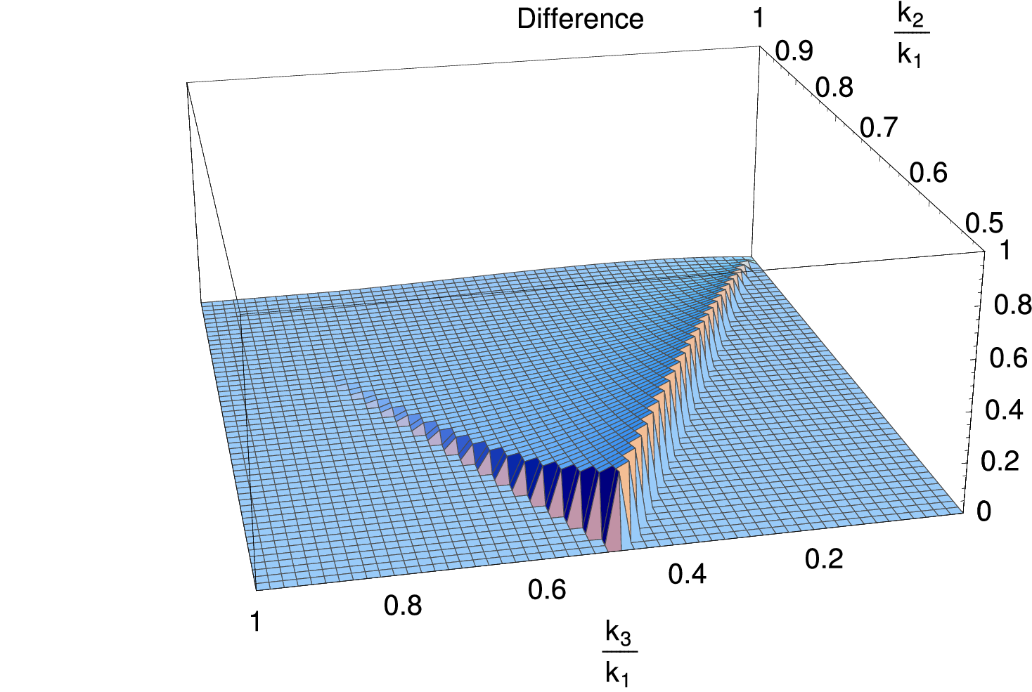
In figure 2, we compare this function with the local shape. The dependence of both functions under a common rescaling of all ’s is fixed to be by scale invariance, so that we can factor out for example. Everything will now depend only on the ratios and , which fix the shape of the triangle in momentum space. For each shape we plot ; this is the relevant quantity if we are interested in the relative importance of different triangular shapes. The square of this function gives the signal to noise contribution of a particular shape in momentum space [78]. We see that for the function (84), the signal to noise is concentrated on equilateral configurations, while squeezed triangles with one side much smaller than the others are the most relevant for the local shape.


VI Conclusion
In this review, the bispectrum of curvature perturbation is calculated using the in-in formalsim and the delta-N formalism. There are two distinct contributions to the bispectrum. One is coming from a non-linear relation between the curvature perturbation and quantum fluctuations of a field at the horizon crossing. In this case the non-linearities come from the evolution of this field outside the horizon. Being local in a position space, the shape of the bispectrum is highly non-local in a Fourie space having a maximum signal for the squeezed configuration . The other contribution is coming from the bispectrum of quantum fields generated under horizon scales. In models in which the non-Gaussianity is generated by derivative interactions such as DBI inflation and k-inflation models, we have correlation among modes of comparable wavelength in all models and these interactions become exponentially irrelevant when the modes go out of the horizon because both time and spatial derivatives become small, so that all the correlation is among modes freezing almost at the same time. Then the bispectrum has a peak at the equilateral configuration .
In order to put constraints on the bispectrum from CMB observations, it is necessary to construct an estimator that uses a model prediction for the bispectrum as an template. For the local-type non-Gaussianity and the equilateral non-Gaussianity, the constraints obtained in WMAP 7-year results are [80]
| (85) |
at confidence level. Recently, it has been found that Large Scale Structure (LSS) can give a similar level of constraints on the local type non-Gaussianity from the scale-dependent bias effects on the halo power spectrum [83] while this effect is absent in the equilateral non-Gaussianity [84, 85]. The constraint on is obtained from SDSS as [86] and combining it to WMAP 7-year results, we get [80]. Thus currents observations are consistent with Gaussian primordial curvature perturbations but future experiments such as Planck will give much tighter constraints and we may be able to detect a deviation from Gaussianity which has a huge impact on early universe models.
There are a lot issues that are not covered by this review. We will mention some of the issues here:
- •
Trispectrum
In this review, we concentrated on the leading order non-Gaussianity, i.e. the bispectrum but it has been recognized that the trispectrum could give a useful information to distinguish between many possible models that predict large non-Gaussianity. For the local non-Gaussianity, we can easily extend the model by expanding up to the third order . The trispetrum is characterized by two parameters and [17, 77, 28]. The constraints on these parameters are rather weak, and from WMAP 5-year results at confidence level [87]. But again the Planck will improve these significantly [88]. The full trispectrum in DBI inflation at the leading order in small sound speed limit has been obtained [25, 89, 90, 91]. Unlike the bispectrum, there are still two degrees of freedom even for the equilateral configurations and also the form of the trispectrum is too complicated to be used for the estimator. It is necessary to develop approximations for the shape of the trispectrum in DBI inflation as is done for the bispectrum. - •
Multi-field inflation
In single field inflation models with a standard kinetic term, the resulting non-Gaussianity is small suppressed by slow-roll parameters. However, in multi-field models, it is possible to have large local non-Gaussianity due to non-linear dynamics of fields outside horizon. The delta-N formalism is easy to be extended to multi-field models and there have been extensive study of non-Gaussianity in multi-field models using the delta-N formalism (see for example [92] and references therein). Multi field effects are also important in DBI inflation. In DBI inflation, fluctuations along the entropy directions of the fields that are orthogonal to the field trajectory have the same sound speed as the adiabatic fluctuations along the field trajectory [31, 32, 30, 93]. If the trajectory makes a turn in a field space, this converts the entropy perturbations to the curvature perturbations. Although the bispectrum is enhanced by this conversion, the enhancement of the power spectrum is stronger and becomes smaller in multi-field models, which help ease stringent constraints on DBI inflation models in string theory [31]. It has been shown that the trispectrum is enhanced for a given [94, 95]. It is also possible that the multi-field effects modify the bipsectrum for quantum field at the horizon crossing. In the so-called quasi-single inflation models [96], the entropy perturbations develops large non-Gaussianity. The conversion of entropy perturbations to the curvature perturbation can happen near the horizon crossing and during this transition the shape of the bispectrum can be modified in a non-trivial way.
There are many other possibilities to get large non-Gaussianity of quantum fields such as a feature in inflaton potentials [26, 97]. All these models predict distinct shapes of the bispectrum and trispectrum. In the future, we may be able to exploit CMB and LSS data to distinguish between many possible early universe models via non-Gaussianity.
Acknowledgements.
We would like to thank the authors of Ref. [79] for giving us a permission to use Fig.1 and Fig.2 in this article. KK is supported by the UK’s Science & Technology Facilities Council, the European Research Council and Research Councils UK.References
- [1] http://www.rssd.esa.int/index.php?project=Planck (2010).
- [2] V. Acquaviva, N. Bartolo, S. Matarrese, and A. Riotto, Nucl. Phys. B667, 119 (2003), eprint astro-ph/0209156.
- [3] J. M. Maldacena, JHEP 05, 013 (2003), eprint astro-ph/0210603.
- [4] A. D. Linde and V. F. Mukhanov, Phys. Rev. D56, 535 (1997), eprint astro-ph/9610219.
- [5] N. Bartolo, S. Matarrese, and A. Riotto, Phys. Rev. D65, 103505 (2002), eprint hep-ph/0112261.
- [6] F. Bernardeau and J.-P. Uzan, Phys. Rev. D66, 103506 (2002), eprint hep-ph/0207295.
- [7] F. Bernardeau and J.-P. Uzan, Phys. Rev. D67, 121301 (2003), eprint astro-ph/0209330.
- [8] G. Dvali, A. Gruzinov, and M. Zaldarriaga, Phys. Rev. D69, 023505 (2004a), eprint astro-ph/0303591.
- [9] P. Creminelli, JCAP 0310, 003 (2003), eprint astro-ph/0306122.
- [10] M. Alishahiha, E. Silverstein, and D. Tong, Phys. Rev. D70, 123505 (2004), eprint hep-th/0404084.
- [11] A. Gruzinov, Phys. Rev. D71, 027301 (2005), eprint astro-ph/0406129.
- [12] K. Enqvist, A. Jokinen, A. Mazumdar, T. Multamaki, and A. Vaihkonen, Phys. Rev. Lett. 94, 161301 (2005a), eprint astro-ph/0411394.
- [13] A. Jokinen and A. Mazumdar, JCAP 0604, 003 (2006), eprint astro-ph/0512368.
- [14] K. Enqvist, A. Jokinen, A. Mazumdar, T. Multamaki, and A. Vaihkonen, JCAP 0503, 010 (2005b), eprint hep-ph/0501076.
- [15] D. H. Lyth, JCAP 0511, 006 (2005), eprint astro-ph/0510443.
- [16] M. P. Salem, Phys. Rev. D72, 123516 (2005), eprint astro-ph/0511146.
- [17] D. Seery and J. E. Lidsey, JCAP 0701, 008 (2007), eprint astro-ph/0611034.
- [18] D. Seery and J. E. Lidsey, JCAP 0506, 003 (2005a), eprint astro-ph/0503692.
- [19] D. Seery and J. E. Lidsey, JCAP 0509, 011 (2005b), eprint astro-ph/0506056.
- [20] M. Sasaki, J. Valiviita, and D. Wands, Phys. Rev. D74, 103003 (2006), eprint astro-ph/0607627.
- [21] K. A. Malik and D. H. Lyth, JCAP 0609, 008 (2006), eprint astro-ph/0604387.
- [22] N. Barnaby and J. M. Cline, Phys. Rev. D73, 106012 (2006), eprint astro-ph/0601481.
- [23] L. Alabidi and D. Lyth, JCAP 0608, 006 (2006), eprint astro-ph/0604569.
- [24] X. Chen, M.-x. Huang, S. Kachru, and G. Shiu, JCAP 0701, 002 (2007a), eprint hep-th/0605045.
- [25] X. Chen, M.-x. Huang, and G. Shiu, Phys. Rev. D74, 121301 (2006), eprint hep-th/0610235.
- [26] X. Chen, R. Easther, and E. A. Lim, JCAP 0706, 023 (2007b), eprint astro-ph/0611645.
- [27] L. Alabidi, JCAP 0610, 015 (2006), eprint astro-ph/0604611.
- [28] C. T. Byrnes, M. Sasaki, and D. Wands, Phys. Rev. D74, 123519 (2006), eprint astro-ph/0611075.
- [29] F. Arroja and K. Koyama, Phys. Rev. D77, 083517 (2008), eprint 0802.1167.
- [30] F. Arroja, S. Mizuno, and K. Koyama, JCAP 0808, 015 (2008), eprint 0806.0619.
- [31] D. Langlois, S. Renaux-Petel, D. A. Steer, and T. Tanaka, Phys. Rev. Lett. 101, 061301 (2008a), eprint 0804.3139.
- [32] D. Langlois, S. Renaux-Petel, D. A. Steer, and T. Tanaka, Phys. Rev. D78, 063523 (2008b), eprint 0806.0336.
- [33] M. Sasaki, Prog. Theor. Phys. 120, 159 (2008), eprint 0805.0974.
- [34] C. T. Byrnes, K.-Y. Choi, and L. M. H. Hall, JCAP 0810, 008 (2008), eprint 0807.1101.
- [35] C. T. Byrnes, K.-Y. Choi, and L. M. H. Hall, JCAP 0902, 017 (2009), eprint 0812.0807.
- [36] S. Yokoyama, T. Suyama, and T. Tanaka, JCAP 0707, 013 (2007), eprint 0705.3178.
- [37] S. Yokoyama, T. Suyama, and T. Tanaka, Phys. Rev. D77, 083511 (2008), eprint 0711.2920.
- [38] B. Dutta, L. Leblond, and J. Kumar, Phys. Rev. D78, 083522 (2008), eprint 0805.1229.
- [39] A. Naruko and M. Sasaki, Prog. Theor. Phys. 121, 193 (2009), eprint 0807.0180.
- [40] T. Suyama and M. Yamaguchi, Phys. Rev. D77, 023505 (2008), eprint 0709.2545.
- [41] T. Suyama and F. Takahashi, JCAP 0809, 007 (2008), eprint 0804.0425.
- [42] X. Gao, JCAP 0806, 029 (2008), eprint 0804.1055.
- [43] H. R. S. Cogollo, Y. Rodriguez, and C. A. Valenzuela-Toledo, JCAP 0808, 029 (2008), eprint 0806.1546.
- [44] Y. Rodriguez and C. A. Valenzuela-Toledo (2008), eprint 0811.4092.
- [45] K. Ichikawa, T. Suyama, T. Takahashi, and M. Yamaguchi, Phys. Rev. D78, 023513 (2008), eprint 0802.4138.
- [46] C. T. Byrnes, JCAP 0901, 011 (2009), eprint 0810.3913.
- [47] S. Li, Y.-F. Cai, and Y.-S. Piao, Phys. Lett. B671, 423 (2009), eprint 0806.2363.
- [48] D. Langlois, F. Vernizzi, and D. Wands, JCAP 0812, 004 (2008c), eprint 0809.4646.
- [49] C. Hikage, K. Koyama, T. Matsubara, T. Takahashi, and M. Yamaguchi (2008), eprint 0812.3500.
- [50] M. Kawasaki, K. Nakayama, T. Sekiguchi, T. Suyama, and F. Takahashi, JCAP 0811, 019 (2008), eprint 0808.0009.
- [51] P. Creminelli and L. Senatore, JCAP 0711, 010 (2007), eprint hep-th/0702165.
- [52] K. Koyama, S. Mizuno, F. Vernizzi, and D. Wands, JCAP 0711, 024 (2007), eprint 0708.4321.
- [53] E. I. Buchbinder, J. Khoury, and B. A. Ovrut, Phys. Rev. Lett. 100, 171302 (2008), eprint 0710.5172.
- [54] J.-L. Lehners and P. J. Steinhardt, Phys. Rev. D77, 063533 (2008a), eprint 0712.3779.
- [55] J.-L. Lehners and P. J. Steinhardt, Phys. Rev. D78, 023506 (2008b), eprint 0804.1293.
- [56] A. Misra and P. Shukla, Nucl. Phys. B810, 174 (2009), eprint 0807.0996.
- [57] Q.-G. Huang, JCAP 0906, 035 (2009), eprint 0904.2649.
- [58] J. Khoury and F. Piazza, JCAP 0907, 026 (2009), eprint 0811.3633.
- [59] L. Verde, L.-M. Wang, A. Heavens, and M. Kamionkowski, Mon. Not. Roy. Astron. Soc. 313, L141 (2000), eprint astro-ph/9906301.
- [60] L.-M. Wang and M. Kamionkowski, Phys. Rev. D61, 063504 (2000), eprint astro-ph/9907431.
- [61] E. Komatsu and D. N. Spergel, Phys. Rev. D63, 063002 (2001), eprint astro-ph/0005036.
- [62] A. A. Starobinsky, JETP Lett. 42, 152 (1985).
- [63] M. Sasaki and E. D. Stewart, Prog. Theor. Phys. 95, 71 (1996), eprint astro-ph/9507001.
- [64] D. H. Lyth, K. A. Malik, and M. Sasaki, JCAP 0505, 004 (2005), eprint astro-ph/0411220.
- [65] D. H. Lyth and Y. Rodriguez, Phys. Rev. Lett. 95, 121302 (2005), eprint astro-ph/0504045.
- [66] T. Tanaka, T. Suyama, and S. Yokoyama (2010), eprint 1003.5057.
- [67] D. S. Salopek and J. R. Bond, Phys. Rev. D42, 3936 (1990).
- [68] M. Sasaki and T. Tanaka, Prog. Theor. Phys. 99, 763 (1998), eprint gr-qc/9801017.
- [69] D. Wands, K. A. Malik, D. H. Lyth, and A. R. Liddle, Phys. Rev. D62, 043527 (2000), eprint astro-ph/0003278.
- [70] C. T. Byrnes, K. Koyama, M. Sasaki, and D. Wands, JCAP 0711, 027 (2007), eprint 0705.4096.
- [71] S. Weinberg, Phys. Rev. D72, 043514 (2005), eprint hep-th/0506236.
- [72] M. E. Peskin and D. V. Schroeder (????), reading, USA: Addison-Wesley (1995) 842 p.
- [73] J. Garriga and V. F. Mukhanov, Phys. Lett. B458, 219 (1999), eprint hep-th/9904176.
- [74] A. J. Christopherson and K. A. Malik (2008), eprint 0809.3518.
- [75] F. Arroja and M. Sasaki (2010), eprint 1002.1376.
- [76] R. Arnowitt, S. Deser, and C. W. Misner, Phys. Rev. 117, 1595 (1960).
- [77] D. Seery, J. E. Lidsey, and M. S. Sloth, JCAP 0701, 027 (2007), eprint astro-ph/0610210.
- [78] D. Babich, P. Creminelli, and M. Zaldarriaga, JCAP 0408, 009 (2004), eprint astro-ph/0405356.
- [79] P. Creminelli, A. Nicolis, L. Senatore, M. Tegmark, and M. Zaldarriaga, JCAP 0605, 004 (2006), eprint astro-ph/0509029.
- [80] E. Komatsu et al. (2010), eprint 1001.4538.
- [81] D. H. Lyth, C. Ungarelli, and D. Wands, Phys. Rev. D67, 023503 (2003), eprint astro-ph/0208055.
- [82] G. Dvali, A. Gruzinov, and M. Zaldarriaga, Phys. Rev. D69, 083505 (2004b), eprint astro-ph/0305548.
- [83] N. Dalal, O. Dore, D. Huterer, and A. Shirokov, Phys. Rev. D77, 123514 (2008), eprint 0710.4560.
- [84] A. Taruya, K. Koyama, and T. Matsubara, Phys. Rev. D78, 123534 (2008), eprint 0808.4085.
- [85] L. Verde and S. Matarrese, Astrophys. J. 706, L91 (2009), eprint 0909.3224.
- [86] A. Slosar, C. Hirata, U. Seljak, S. Ho, and N. Padmanabhan, JCAP 0808, 031 (2008), eprint 0805.3580.
- [87] J. Smidt et al. (2010), eprint 1001.5026.
- [88] N. Kogo and E. Komatsu, Phys. Rev. D73, 083007 (2006), eprint astro-ph/0602099.
- [89] X. Chen, B. Hu, M.-x. Huang, G. Shiu, and Y. Wang (2009), eprint 0905.3494.
- [90] F. Arroja, S. Mizuno, K. Koyama, and T. Tanaka, Phys. Rev. D80, 043527 (2009), eprint 0905.3641.
- [91] S. Renaux-Petel, JCAP 0910, 012 (2009), eprint 0907.2476.
- [92] C. T. Byrnes and G. Tasinato, JCAP 0908, 016 (2009), eprint 0906.0767.
- [93] S. Mizuno, F. Arroja, K. Koyama, and T. Tanaka, Phys. Rev. D80, 023530 (2009a), eprint 0905.4557.
- [94] S. Mizuno, F. Arroja, and K. Koyama, Phys. Rev. D80, 083517 (2009b), eprint 0907.2439.
- [95] X. Gao, M. Li, and C. Lin, JCAP 0911, 007 (2009), eprint 0906.1345.
- [96] X. Chen and Y. Wang (2009), eprint 0911.3380.
- [97] X. Chen, R. Easther, and E. A. Lim (2008), eprint arXiv:0801.3295 [astro-ph].