Superconductivity generated by coupling to a Cooperon in a 2-dimensional array of 4-leg Hubbard ladders
Abstract
Starting from an array of four-leg Hubbard ladders weakly doped away from half-filling and weakly coupled by inter-ladder tunneling, we derive an effective low energy model which contains a partially truncated Fermi surface and a well defined Cooperon excitation formed by a bound pair of holes. An attractive interaction in the Cooper channel is generated on the Fermi surface through virtual scattering into the Cooperon state. Although the model is derived in the weak coupling limit of a four-leg ladder array, an examination of exact results on finite clusters for the strong coupling t-J model suggests the essential features are also present for a strong coupling Hubbard model on a square lattice near half-filling.
pacs
PACS numbers: 71.10.Pm, 72.80.SkI Introduction
The microscopic mechanism that generates high temperature superconductivity in the cuprates continues to be controversial. One set of proposals is based on the analogy with heavy fermion metals where a superconducting dome is observed surrounding the quantum critical point (QCP) that arises as antiferromagnetism is suppressed by an external parameter such as pressure.[1] In this case the pairing glue arises from the exchange of the soft longitudinal antiferromagnetic fluctuations in the vicinity of the QCP. In the cuprates doping plays the role of the external parameter and there are several proposals for the nature of the QCP that appears near optimal doping involving fluctuations in various order parameters e.g. nematic,[2] d-density wave[3] and orbital currents[4] in addition to antiferromagnetism.[5] A second set goes back to Anderson’s very early proposal that the strong singlet nearest neighbor correlations in the 2-dimensional Heisenberg antiferromagnet generates pairing when doped holes are introduced. The advocates of this resonant valence bond (RVB) mechanism point to the strong asymmetry in the cuprate phase diagram between the physical behavior on the under- and overdoped sides of optimal doping and the QCP. This contrasts strongly with the symmetric dome observed in heavy fermions. Further the highly anomalous physical properties that characterize the pseudogap phase at underdoping are associated with a short range spin liquid in the cleanest cuprate materials, e.g. YBa2Cu4O8 and HgBa2CuO4+x. Nonetheless strong correlations and the absence of a broken translational symmetry in the pseudogap phase have proved to be formidable obstacles to constructing a comprehensive microscopic RVB theory for underdoped cuprates. For more details see several recent reviews.[6, 7, 8, 9]
Several years ago we proposed a 2-dimensional array of weak coupled 2-leg Hubbard ladders as an example of a model where occurs a truncation of the full Fermi surface to pockets associated with hole or electron doping in a system without broken symmetry.[10] Subsequently this model led to a phenomenological ansatz for the propagator in underdoped cuprates starting from a renormalized mean field description of an undoped RVB spin liquid insulator.[11] This phenomenological propagator has been recently used successfully to fit a range of experiments covering many anomalous properties of the pseudogap phase.[12, 13, 14, 15, 16, 17, 18] In this paper we extend our earlier analysis to the case of an array of lightly doped 4-leg Hubbard ladders with an onsite weak interaction. Our goal is to construct a tractable 2-dimensional model with a partially truncated Fermi surface in which d-wave pairing arises on the residual Fermi surface through scattering in the Cooper channel.
Earlier numerical renormalization group studies on the 2-dimensional Hubbard model were interpreted as pointing towards a similar pairing mechanism.[19, 20] A key feature of the present model is the presence of a finite energy Cooperon resonance in the pseudogap which is generated in association with the partial truncation of the Fermi surface. D-wave pairing follows on the remnant Fermi surface through the coupling to the Cooperon.
II Four Leg Hubbard Ladders
The properties of a single 4-leg Hubbard ladder with open boundaries have been studied extensively in both the weak and strong coupling limits. We consider here the former with equal nearest neighbor hopping , along the legs and rungs. In this case the 4 bands split into two band pairs. The inner pair, , are standing waves on the rungs with wavevectors . At half filling the corresponding Fermi wavevectors are and leading to a common Fermi velocity, . The outer band pair, , have Fermi wavevectors and and a smaller Fermi velocity, .
We obtain a band structure of four bands with energies
| (1) | |||||
| (2) |
where represents the dispersion along the ladder. The annihilation (creation) operators of electrons of the outer and inner bands, denoted as and respectively, are
| (3) | |||||
| (5) | |||||
| (7) | |||||
| (9) |
where is the corresponding annihilation operator of an electron on the n-th leg of the ladder.
 |
 |
Close to half filling the Fermi velocities of the outer band pair labeled by are smaller than those of the inner bands labeled by , so that in the presence of interactions the effective dimensionless coupling constants for electrons in the inner bands are smaller than those for the outer bands. In the weak coupling limit, i.e. an onsite interaction characterized by , this Fermi velocity difference leads to a large difference in the characteristic energy scales and to a decoupling of the RG flows of the two band pairs. The outer band pair has the larger critical energy scale and flows to strong coupling first as the energy scale is lowered.[21, 22, 23] The inner band pair has a lower critical scale. Therefore in the first approximation one can treat inner and outer bands of individual 4-leg ladders as decoupled from each other. Then each band pair will effectively constitute a two-leg ladder. It is well known that two-leg ladders acquire spectral gaps for quite general interaction patterns. For the inner bands the smaller dimensionless couplings lead to smaller spectral gaps. At half filling each band pair is exactly half filled and behaves as a half filled 2-leg Hubbard ladder. The difference in the energy scales leads to a finite doping range where all the doped holes enter the inner band pair and the outer band pair remains exactly half filled. We note in passing that similar behavior is found also in the strong coupling limit, .[24]
Given that a 4-leg ladder can be reduced to two 2-leg ladders, we will now recall some basic facts about 2-leg ladders. For general interactions they become either Luttinger liquids or dynamically generate spectral gaps. In the latter case an increased symmetry appears at small energies where a half filled 2-leg ladder can be well described by the O(8) Gross-Neveu model.[25] The Gross-Neveu model is exactly solvable for all semi-simple symmetry groups and a great deal is known about its thermodynamics and correlation functions. In the SO(8) case the correlation functions were studied in Refs. (26, 27). Since the model itself has Lorentz symmetry, all excitation branches have relativistic dispersion laws:
| (10) |
The spectrum consists of three octets of particles of mass and a multiplet of 29 excitons with mass . Two octets consist of quasi-particles of different chirality transforming according to the two irreducible spinor representations of SO(8), while the third octet consists of vector particles. The latter include magnetic excitations as well as the Cooperon (a particle with charge ). The 16 kink fields, carrying charge, spin, orbit, and parity indices, are direct descendants of the original electron lattice operators on the ladders.
The SO(8) GN model describes several different phases related to one another by particle-hole transformations. Which phase is realized depends on the bare interaction. In this paper we assume that it is in the so-called D-Mott phase (in the terminology of Ref. 25). On the two two-leg ladders ( and ), the superconducting (SC) order parameters are given by
| (11) | |||||
| (12) |
The distinct feature of the half filled ladder is that this order parameter is purely real and has a Z2 symmetry. However, the symmetry is restored to U(1) and the phase stiffness becomes non-zero as soon as doping is introduced. It is an interesting feature of the SO(8) GN model that the only mode which becomes gapless at finite doping is the Cooperon. Neither magnetic excitations, nor quasi-particles become gapless.[29] When the doping increases the SO(8) GN model gradually crosses over to the SO(6) GN one plus the U(1) Gaussian model. The latter model describes the fluctuations of the superconducting phase. The effective low energy bosonized Lagrangian density for the Cooperon field, , is
| (13) |
where is the field dual to . (Here – according to Ref. (28) – the Luttinger parameter depends weakly on doping and is always in the range . On the other hand, the phase velocity is strongly doping dependent.)
For values of doping close to the Cooperon band edge () spectral curvature is important and the action given in Eqn. 13 is inadequate. A better description of the Cooperon dynamics is given by the sine-Gordon model
| (14) |
where . The mass term here can be thought to arise as follows in a mean field way from the SO(8) Gross-Neveu model. The SO(8) Gross-Neveu model can be written in terms of fundamental fermions (which are non-local with respect to the original fermions in the problem) with an interaction term of the form
| (15) |
Here and and is a Pauli matrix acting in space. The four fundamental fermions correspond to the different degrees of freedom in SO(8): charge, spin, orbital, parity. The Cooperon (charge) we take to be given by . With a finite chemical potential lowering the Cooperon gap, the fluctuations of the Cooperon will be strongest. Invoking mean field theory, we thus replace for by its expectation value. The resulting bosonization of the remaining degree of freedom results in the sine-Gordon model.
III Superconductivity of Arrays of Four-Leg Ladders: Two Scenarios
Having elucidated the properties of individual 4-leg ladders, we now consider an array of such ladders. We assume initially that the electron-electron interaction acts only inside individual ladders and is much smaller than the bandwidth . It is also assumed that (the inter-ladder tunneling). We imagine two scenarios. In the first we assume is on the same order as , the gap on the inner bands of the four leg ladder, but much smaller than , the gap on the outer bands. In this case coupling the ladders together lead to small Fermi pockets, very much like in Ref.(10). However in this case the pockets are found near . The residual coupling between these Fermi pockets and the A-cooperons then leads to superconductivity in the A-bands. And because of a proximity effect, the superconductivity of the A-bands induces superconductivity in the B-bands.
In the second scenario, we assume . In this case wipes out the effects of interactions on the A-bands. Coupling them together then gives us an anisotropic two dimensional Fermi liquid. But as is much smaller than , the Cooperons on the outer bands at zeroth order remain unperturbed. The coupling then between the anisotropic Fermi liquid and the B-Cooperons induces superconductivity in the system as a whole. This superconductivity is d-wave in nature.
We now elaborate on these two scenarios.
III.1 Scenario I
We treat the interladder hopping through a random phase approximation (RPA) analysis of the interladder hopping. The form of the hopping is taken to be long range
| (16) |
where run over the legs of an individual ladder and and mark the ’th and ’th ladders. By particle-hole symmetry the hopping is assumed to have peaks both near and where is the inverse lattice vector perpendicular to the ladders. In particular the hopping takes the form
| (17) |
where and (i.e. no (additional) hopping within a ladder).
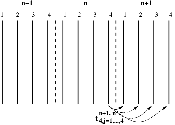
By treating in an RPA approach, we find that the single particle Green’s function takes the form
| (18) | |||||
| (20) |
where
| (23) | |||||
| (27) | |||||
| (29) | |||||
| (31) |
and and . We have assumed the hopping is real and that the low energy contribution to comes from the -bands as . Thus are the Green’s functions of the -band electrons on a given 4-leg ladder. As we have discussed in the previous section are no more than the bonding/anti-bonding electron Greens functions for a 2-leg ladder. The RPA does not mix and as the weights of the two are found near differing Fermi wavevectors (i.e. we can take safely for all ). The presence of and act as structure factors which cause the quasiparticle weight at various to be negligible. While the denominator of has the periodicity of the reduced Brillouin zone i.e. and are identified) these structure functions merely have the periodicity of the original zone i.e. and are identified).
The Green’s functions for at zero chemical potential are given by
| (32) |
where the are defined in Eqn. 1. At a chemical potential, , that does not exceed the gap, is given by
 |
 |
The excitations are then given by the locations of the poles in . These poles then imply that the excitations have the dispersion relation
| (33) |
For sufficiently large a Fermi surface forms (found by solving ) consisting of electron and hole pockets. The type of pocket is determined by the sign of the effective hopping
| (34) | |||||
| (35) |
In our conventions a positive chemical potential favors hole pocket formation while disfavoring electron pockets. As grows beyond this minimal value, the pockets grow in size. We take the hopping such that
| (36) |
where is the small parameter guaranteeing that the RPA is a good approximation.
The dispersion relations of the quasi-particles near the hole pockets are
| (37) |
where , , , , and .
In Figure 3 are plotted the expected Fermi pockets. On the l.h.s. of Figure 3 are plotted the pockets found at zero chemical potential while on the r.h.s. are plotted the pockets for a chemical potential such that . For such a condition one obtains only hole pockets. We see that hole pockets occur in the vicinity of .
III.1.1 Luttinger sum rule
The Luttinger sum rule (LSR) for the single particle Green’s functions at the particle hole symmetric point takes the form
| (38) |
where is the electron density. The corresponding Luttinger surface of is defined as the loci of points in -space where changes sign. These sign changes occur both at the poles and the zeros of . In order to apply the Luttinger sum rule, we must take to be one of , i.e. we must apply the LSR to each band separately (see Eqn. (18) for the definition of ). (We only apply the LSR to the electrons in the A-bands – the LSR also holds separately for electrons in the B-bands.)
At the particle-hole symmetric point, zeros are present in along the lines . In the absence of pockets the LSR is satisfied because of these zeros. And when becomes strong enough so that pockets form, the appearance of equally size electron and hole pockets on either side of ensure that the Luttinger sum rule continues to hold.
Introducing a finite chemical potential (with ) leaves the LSR violated as expressed in Eqn. (38). However it continues to hold in a modified form. Because in a finite chemical potential, the ladder Greens functions are given by , the LSR holds if we consider the sign changes the Green’s function undergoes not at but at .
III.1.2 Superconducting Instability
The residual interactions between the Fermi pockets and the Cooperons will lead to instabilities in the RPA solutions as temperature goes to zero. Provided a finite chemical potential is present the leading instability will be to a superconducting state. While gapless quasi-particles only exist in the A-bands, both A and B bands will go superconducting simultaneously. The general form of the Cooperon-quasiparticle interaction is
| (39) | |||||
| (41) | |||||
| (43) |
Here is the length of the ladders, is the interladder spacing, and is the number of ladders in the array. are the Cooperon fields whose bare propagators are defined as
| (44) |
We see that has the dimensionality of energylength2 and has the dimensionality of energylength1/2.
The different terms in Eqn. (39) have different origins. The strongest interactions are presumably as this term already exists for uncoupled ladders. Inter-ladder interactions, such as interladder Coulomb repulsion, also contribute to . However interladder hoping does not – this contribution is suppressed due to a mismatch between the Fermi momenta of the and bands. The coupling is smaller than : it arises only in second order perturbation theory from intraladder interactions and from presumed weak inter-ladder Coulomb interactions.
The pair susceptibility for the quasiparticles in an RPA approximation is given by
| (45) | |||||
| (47) |
We have assumed that the couplings and are such that we can ignore their dependence on and . Here is the Cooper bubble:
| (48) |
Here are the bare dispersions of the quasi-particles. As , develops a logarithmic divergence: .
The pair susceptibility for the Cooperons fields has a similar RPA form:
| (51) | |||||
where . The superconducting instability occurs when the denominator in Eqns. (18 and 32) vanishes at , that is
| (52) |
We note that this vanishing occurs simultaneously in all channels. If (though interladder Coulomb repulsion is repulsive, the interactions between quasi-particles on a given ladder is attractive leaving the sign of g indeterminate) the instability occurs only when the chemical potential approaches sufficiently close to so that the resulting effective interaction becomes attractive. This chemical potential corresponds to minimal doping at which the superconductivity appears. Taking , the corresponding transition temperature takes the form
| (53) |
where . If we suppose that and are such that we only have hole pockets, the density of dopants is equal to
| (54) |
If we denote the critical doping as where the A-Cooperon becomes soft, we see that the transition temperature behaves as as approaches , that is to say, the transition temperature has a strong dependence on doping. It should be emphasized that this critical doping as defined above does not coincide with the optimal doping as typically understood. Optimal doping can be thought of as the doping level associated with a change in the Fermi surface topology. However in this understanding our model always remains in the underdoped regime since the quasiparticle Fermi surfaces remain small as far as the interladder tunneling remains much smaller than the gap of the outer (B) band pair.
III.2 Scenario 2
We now consider the second scenario where . Because is much larger than but smaller than , the effects of the interactions are wiped out in the A-bands while preserved in the B-bands. In particular a gapful Cooperon still exists on the B-bands while the coupled A-bands appear as an anisotropic two dimensional Fermi liquid.

We can distinguish two parameter ranges in this scenario. At small dopings , the B-Cooperons remain gapped. The effective Hamiltonian for the two dimensional Fermi liquid in the A-bands and the Cooperons in the B-bands appears as
| (55) | |||||
| (57) | |||||
| (59) |
where is given in Eqn. (1) and in Eqn. (23). We illustrate the two dimensional Fermi surface of the A-bands in Figure 4.
The form of the quasi-particle-Cooperon interaction is that of Eqn. (45) (though of course, now we have no A-Cooperon and so this coupling is absent). This system, like in Scenario 1, has a pairing instability to superconductivity. The pairing susceptibilities in an RPA approximation take a similar form as for Scenario 1:
| (60) | |||||
| (62) |
where is defined as in Eqn. (51).
As we no longer have pockets as in Scenario 1, but instead have an anisotropic 2D Fermi liquid whose Fermi surface consists of slightly deformed lines (see Figure 4), the divergent with temperature behaviour of now takes the form
| (63) |
Because the A-quasi-particles are already gapless, a finite dopes the A-bands with doping . Thus . If we denote the critical doping, , as the doping when the B-Cooperon becomes soft (i.e. ) and the corresponding doping of the A-bands, we can rewrite the form of the B-Cooperon propagator, , as
| (64) |
Again we emphasize that the critical doping as defined above does not coincide with optimal doping – in this model we are always in the underdoped regime. For this range of doping we obtain a transition temperature of the form
| (65) |
and we see that the critical temperature grows extremely fast with doping, similar to the transition temperature determined in Scenario I.
The second region occurs at , when the holes penetrate into the outer B-bands. Here the O(8) Gross-Neveu model governing the B-bands undergoes a crossover into a Gross-Neveu model. The B-Cooperon propagator at becomes more singular. At the same time the velocity of the phase fluctuations becomes small and these fluctuations can be treated as slow modes. Integrating over the nodal fermions one obtains the effective Lagrangian for the phase fluctuations:
| (68) | |||||
where is a sum over ladders. As we have already noted the parameter is renormalized by the Coulomb interaction to be slightly less than 1. is more dramatically affected, taking the form so that it vanishes at (or equivalently . As a side remark we note that there is an alternative way of presenting the effective Hamiltonian. The above Lagrangian (Eqn. 68) is the continuum limit of the following model:
| (71) | |||||
where are Pauli matrix operators. In the continuum limit becomes the order parameter field . Here . The model presented above is a model of anisotropic spin-1/2 magnet on a 2D lattice with a staggered () and uniform magnetic fields (). This form of the Hamiltonian has been proven to be very convenient for numerical calculations yielding promising results for the transport.[31]
We again estimate the transition temperature using an RPA argument. At the doping of the entire system (both the A and the B bands) is
| (72) |
where is a constant and The detailed form of the Cooperon propagator for a single chain at T=0 can be extracted from Ref 30. However to obtain an estimate for , it is enough to use the finite temperature Luttinger liquid expression for the Cooperon propagator:
| (73) |
where is a numerical constant. Thus
| (74) |
Substituting the latter expression into RPA expressions for the pairing susceptibilities (Eqns. 60) we obtain an estimate for the critical temperature upon doping as follows:
| (75) |
This dependence on the doping is much weaker than (Eqn. 73). It holds in the region where phase fluctuations are already strong.
Thus we have obtained two regimes with different doping dependence of . The first one is the BCS-like with given by Eqn. (65). It corresponds to lowest doping levels. The other regime, which in our model still describes a situation an anisotropic 1D-like Fermi surface, is the regime with strong phase fluctuations. The mean field transition temperature in this regime is given by Eqn. (75). A further increase of doping presumably will lead to a change in the Fermi surface topology and is not considered in this paper.
IV Discussion
Phenomenological models based on coupled fermions and bosons similar to that derived here, have been proposed much earlier Refs.(32, 33, 34, 35) to describe the high temperature superconductors. The closest similarity are to the models proposed by Geshkenbein, Ioffe and Larkin[34] and by Chubukov and Tsvelik.[35, 36] Both these phenomenological models examined Fermi arcs centered on the nodal directions, coupled in the d-wave channel to Cooperons associated with the antinodal regions. The model studied in Ref. (34) had dispersionless Cooperons which provided BCS-style coupling for the nodal quasiparticles. The result was a superconducting transition with weak fluctuations, similar to our case. In the model considered in Ref. 35 the Cooperons possessed a one-dimensional dispersion which resulted in strong fluctuations as takes place in our case for . The authors of Refs. 34, 35, 36 considered the fluctuation regime above Tc when the Cooperon energy is close to the chemical potential and drew comparisons to experiments in several underdoped cuprates. The key ingredients controlling superconductivity in the array of 4-leg Hubbard ladders that we have considered in this letter, are a small residual Fermi surface (either pockets as in Scenario I or arcs as in Scenario II), which is coupled in the d-wave Cooper channel to a finite energy Cooperon associated with the pseudogap responsible for the partial truncation of the Fermi surface. The properties of a weak coupling 4-leg Hubbard ladder near to half-filling are used to obtain these key ingredients. Our goal is to derive a tractable model containing the important features that are relevant to high temperature superconductivity in the cuprates. In order to assess the relevance of our model to this goal, clearly one must examine whether these key ingredients are present in a two dimensional Hubbard model on a square lattice near half-filling.
As we mentioned above, earlier numerical renormalization group studies on the 2-dimensional Hubbard model were interpreted as pointing towards a similar pairing mechanism arising from enhanced pairing correlations present in a condensate that truncates the Fermi surface in the antinodal regions. There are of course two reservations in these earlier works. Firstly, the one loop approximation in the numerical renormalization group studies limits them to at most moderately strong onsite repulsive interactions. Secondly, the renormalization group studies per se break down when the scattering vertices flow to strong coupling and the nature of the resulting low energy or low temperature effective action is a difficult problem which could only be surmised rather than explicitly derived. These two weaknesses make it imperative to examine the question whether these key ingredients are present also for strong coupling.
The most reliable strong coupling calculations are exact diagonalization studies of strong coupling Hamiltonians. The only limitation is the finite cluster size which currently is limited to small clusters containing up to 32 sites and 1,2 and 4 holes. Leung and his collaborators Refs. 37, 38, 39 have reported a series of calculations for these clusters using the strong coupling t-J model and its extensions to include longer range hopping and interactions. We begin with a recap of the main conclusions of these calculations. The allowed set of k-points in a 32-site cluster with periodic boundary conditions contain both the four nodal () and two antinodal points () and (). A single hole enters at a nodal point. For two holes there are two different states that are possible groundstates depending on the parameter values. For the plain t-J model with only nearest neighbour hopping a 2-hole bound pair state with d() symmetry is the groundstate on the 32-site cluster for J/t 0.28. The binding energy is quite small at J/t = 0.3 but grows with increasing J/t. An extrapolation from finite size clusters to the infinite lattice however suggests that the pair state is no longer the groundstate at J/t =0.3, but an excited state with an energy of approximately 0.17t.[37] The inclusion of longer range interactions and hopping in the t-J model increases the energy of the pair state further and confirms the conclusion that for parameter values relevant to cuprates the groundstate of the cluster has two unbound holes in the nodal states.[38] Extending the calculations to the 32-site clusters with 4 holes, which corresponds to a doping of 1/8, shows all 4 holes entering into nodal states with no signs of pairing correlations.[39] In view of the prominent bound pair excited state for 2 holes, a low energy excited state with two of the holes in a bound state may also be expected here. However at present there is no information on this question to the best of our knowledge.
Leung and collaborators[37, 38, 39] concluded from these calculations that at low densities holes entered the nodal regions, possibly in pockets, and as a result there was no evidence for d-wave pairing correlations in the groundstate for realistic values of the parameters in t-J models. However the analysis presented here suggests a more optimistic conclusion. First we note that the nodal points in the 32-site cluster are very special, because exactly at these points the coupling in a Cooper channel to a d-wave Cooperon vanishes by symmetry. Thus if we interpret the d-wave pair excited state as evidence for a finite energy Cooperon in the t-J model and its extensions, then as the occupied holes at finite doping move out from the exact nodal points, a d-wave pairing attraction is generated through the coupling to this Cooperon, similar to the scenarios we discussed earlier. Note an earlier study for two holes on smaller clusters by Poilblanc and collaborators[40] concluded in favor of the interpretation of the 2-hole bound state as a quasiparticle with charge 2e and spin 0, which would be an actual carrier of charge under an applied electric field. In other words they concluded that a Cooperon is present in the strong coupling t-J model at low doping. A more detailed analysis of the origin of the pairing in this state was published recently by Maier et al.[41] Note the hole density in the case of 2 holes in a 32-site cluster is very low so that the superconducting order we are postulating should coexist with long range antiferromagnetic order. There is considerable evidence both numerical, in variational Monte Carlo calculations, and experimental, in favor of such coexistence, as discussed in the recent review by Ogata and Fukuyama.[9]
We conclude that there is strong evidence that the pairing mechanism in the present model is not confined to weak coupling and ladder lattices, but will also operate in the strong coupling t-J model on a square lattice at low doping.
ATM and RMK acknowledge support by the US DOE under contract number DE-AC02-98 CH 10886. TMR was supported by the Center for Emerging Superconductivity funded by the U.S. Department of Energy, Office of Science and by MANEP network of Swiss National Funds.
References
- [1] N. D. Mathur, F. M. Grosche, S. R. Julian, I. R. Walker, D. M. Freye, R. K. W. Haselwimmer and G. G. Lonzarich, Nature, 394, 39, (1998).
- [2] S. A. Kivelson, I. P. Bindloss, E. Fradkin, V. Oganesyan, J. M. Tranquada, A. Kapitulnik and C. Howald, Rev. Mod. Phys. 75, 1201 (2003).
- [3] S. Chakravarty, R. B. Laughlin, D. K. Morr, C. Nayak, Phys. Rev. B 63, 094503 (2001)
- [4] C. Varma, Phys. Rev. B 63, 14554 (1997).
- [5] the latest summary of these ideas can be found in S. Sachdev, arXiov:0910.0846.
- [6] P. W. Anderson, P. A. Lee, M. Randeria, T. M. Rice, N. Trivedi, and F. C. Zhang; J. Phys.Cond. Mat. 16, R755, (2004)
- [7] B. Edegger, V. N. Muthukumar, C. Gros, Adv.Phys., 56, 927 (2007)
- [8] P. A. Lee, Rep.Prog.Phys. 71, 012501, (2008)
- [9] M. Ogata and H. Fukuyama, Rep.Prog.Phys. 71, 036501, (2008)
- [10] R. M. Konik, T. M. Rice and A. M. Tsvelik, Phys. Rev. Lett. 96, 086407 (2006).
- [11] K.-Y. Yang , T. M. Rice, F.-C. Zhang, Phys. Rev. 73, 174501 (2006).
- [12] K.-Y. Yang, H. B. Yang, P. D. Johnson, T. M. Rice F.-C. Zhang., EPL 86, 37002 (2009).
- [13] H. Yang, J. Rameau, P. D. Johnson, to appear.
- [14] B. Valenzuela and E. Bascones, Phys. Rev. Lett. 98, 227002 (2007)
- [15] E. Illes, E. J. Nicol, and J. P. Carbotte, Phys. Rev. B 79, 100505 (2009)
- [16] J.P.F. LeBlanc, E. J. Nicol, and J. P. Carbotte, Phys. Rev. B 80, 060505 (2009)
- [17] J. P. Carbotte. K.A.G. Fisher, J.P.F. LeBlanc, and E.J.Nicol, arXiv 0909.3814
- [18] J.P.F. LeBlanc, J. P. Carbotte and E.J.Nicol, arXiv 0910.3577
- [19] C. Honerkamp, M. Salmhofer, N. Furukawa, T. M. Rice, Phys. Rev. B 63, 035109 (2001).
- [20] A. Laeuchli, C. Honerkamp, T. M. Rice, Phys. Rev. Lett.92,037006 (2004).
- [21] U. Ledermann, K. Le Hur, T. M. Rice, Phys. Rev. B 62, 16383 (2000).
- [22] M.-S. Chang, I. Affleck, Phys. Rev. B 76, 054521 (2007)
- [23] K. Le Hur, T. M. Rice, Ann. Phys. 324, 1452 (2009).
- [24] F. H. L. Essler and A. M. Tsvelik, Phys. Rev B. 65, 115117 (2002); ibid. 71, 195116 (2005).
- [25] H. L. Lin, L. Balents and M. P. A. Fisher, Phys. Rev. B58, 1794 (1998).
- [26] R. Konik and A. Ludwig, Phys. Rev. B64, 155112 (2001); R. Konik et al., Phys. Rev. B 61, R4983 (2000).
- [27] F. H. L. Essler and R. M. Konik in “From Fields to Strings: Circumnavigating Theoretical Physics”, ed. by M. Shifman, A. Vainshtein and J. Wheather, World Scientific, Singapore (2005); cond-mat/0412421.
- [28] R. Konik, F. Lesage, A. W. W. Ludwig and H. Saleur, Phys. Rev. B 61, 4983 (2000).
- [29] J. Evans and T. Hollowood, Nucl. Phys. Proc. Suppl. 45A (1996) 130; T. Hollowood and J. Evans, unpublished.
- [30] J. S. Caux, P. Calabrese, N. A. Slavnov, J. Stat. Mech, P01008 (2007).
- [31] N. H. Lindner and A. Auerbach, arXiv:0910.4158.
- [32] R. Friedberg, T. D. Lee, Phys. Rev. B 40, 6745 (1989).
- [33] J. Ranninger,J. M. Robin, M. Eschrig, Phys. Rev. Lett.74,4027 (1995).
- [34] V. B. Geshkenbein, L. B. Ioffe, A. I. Larkin Phys. Rev. B 55, 3173 (1997).
- [35] A. V. Chubukov and A. M. Tsvelik, Phys. Rev. Lett. 98, 237001 (2007).
- [36] A. V. Chubukov and A. M. Tsvelik, Phys. Rev. B 76, 100509, (R) (2007).
- [37] A.L.Chernyshev, P.W.Leung and R.J.Gooding, Phys. Rev B 58, 13594 (1998).
- [38] P.W. Leung, Phys. Rev. B 65, 205101 (2002).
- [39] P.W.Leung, Phys. Rev. B 73, 014502 (2006).
- [40] D. Poilblanc, J. Riera, E. Dagotto Phys. Rev. B 49, 12318 (1994).
- [41] T. A. Maier, D. Poilblanc, and D. J. Scalapino, Phys. Rev. Lett. 100, 237001 (2008).