Strong coupling constant from vacuum polarization functions in three-flavor lattice QCD with dynamical overlap fermions
Abstract
We determine the strong coupling constant from a lattice calculation of vacuum polarization functions (VPF) in three-flavor QCD with dynamical overlap fermions. Fitting lattice data of VPF to the continuum perturbative formula including the operator product expansion, we extract the QCD scale parameter . At the boson mass scale, we obtain , where the first error is statistical and the second is our estimate of various systematic uncertainties.
pacs
11.15.Ha,12.38.Gc,12.38.AwI Introduction
Strong coupling constant is one of the fundamental parameters in the Standard Model. Its precise determination from various sources provides a crucial test of Quantum Chromodynamics (QCD). Experimentally, it is obtained through high energy particle scatterings involving quarks, such as (see [1, 2] for a summary), for which perturbative calculation of QCD is possible.
Among other measurements, the hadronic decay rate of tau lepton [3] provides one of the most precise determinations of . The tau-lepton hadronic decay rate is written in terms of a vacuum polarization function (VPF) of weak currents. Since the perturbative QCD calculation cannot be directly applied for physical time-like momentum transfer (or the virtual boson mass) , one considers a total decay rate that involves an integral over . The decay rate is then calculated using three-loop perturbative expansion and the Operator Product Expansion (OPE) to parametrize corrections at low energies. The final error in contains those from the perturbative expansion and uncertainties of condensates appearing in OPE, both of which are non-negligible because the relevant energy scale is of order of 1 GeV, i.e. lower than the tau lepton mass . There is also an assumption of the quark-hadron duality, which is not trivially satisfied.
Theoretically, the perturbative calculation and the extraction of become more transparent if the experimental data for VPF are available at space-like momenta. Although there is no such direct measurement, lattice QCD is able to provide a non-perturbative calculation of VPF at space-like momenta. Since the calculation is based on the first-principles of QCD, for which the input parameters are low-lying hadron spectrum, it gives another method to extract .
Using lattice QCD, one can calculate VPF of vector () and axial-vector () channels from two-point functions of those currents. After a Fourier transformation in four space-time dimensions, VPF can be obtained as a function of space-like momentum squared ranging from zero to the order of lattice cutoff squared. Our recent lattice study with two flavors of dynamical overlap fermions demonstrated that such data can indeed be used to extract combining with a perturbative calculation in the continuum scheme [4]. The result is consistent with other lattice calculations in two-flavor QCD [5, 6].
One of the main advantages of our method is that the calculation can be done on existing gauge configurations produced for light-hadron spectrum [7]. Furthermore, unlike other methods previously applied, there is no need of multi-loop perturbative calculation on the lattice, which is so complicated that one typically has to develop automated tool dedicated for a given lattice action. Finite volume effect is negligible for VPF at relatively large , and discretization effect is carefully studied and is shown to be under control. The method therefore provides a reliable and economical way to extract the most important parameter of QCD, i.e. . A similar idea has also been applied for the charmonium two-point function to determine as well as charm quark mass [9].
In this work, we extend our previous study to the case of realistic three-flavor QCD with dynamical light and strange quarks. We also improve the calculation by employing the conserved current for the overlap fermion [10], which simplifies the possible form of the two-point function as it satisfies the Ward-Takahashi (WT) identity on the lattice. The extraction of VPF is thus made more straightforward. The determination of the strong coupling constant uses the continuum perturbative QCD formula up to four loops and OPE up to terms. The value of the quark condensate is calculated independently and used as an input in this work. The result is translated to the common definition, i.e. , the strong coupling constant of five-flavor QCD in the scheme at the boson mass scale.
Numerical simulations of lattice QCD are carried out with 2+1-flavors of dynamical fermions described by the overlap fermion formulation [11, 12]. We have data at a single lattice spacing with the inverse lattice spacing = 1.83(1) GeV estimated using the static quark potential with an input for the Sommer scale = 0.49 fm (the associated error for this is discussed later). The lattice volume is , which leads to the physical volume about (1.8 fm)(5.4 fm). The gauge configurations are generated in the course of the dynamical overlap fermion simulations by the JLQCD and TWQCD collaborations [13]. The set of up and down quark masses covers the range of (0.2–0.8) and the set of the strange quark mass covers the range of (1.0–1.3) with the physical strange quark mass. The valence quark mass in the calculation of VPF is set equal to the up and down sea quark mass. For each combination of and , we use 260 configurations, each of which is separated by 100 HMC trajectories. Global topological charge of the gauge configurations is fixed to zero, which may induce small finite size effect for long distance physical quantities [14]. We expect that this gives negligible effects on the short distance physics considered in this work.
The rest of the paper is organized as follows. In Section II, we describe the details of the lattice calculation of VPF, including the definition of the overlap fermion used in this work and a construction of the conserved current for the overlap fermion. Section III discusses the fit of VPF to the perturbative formula. The possible systematic errors are discussed in Section IV, followed by our final results. Our conclusions are given in Section V.
II Lattice calculation of vacuum polarization functions
In the continuum theory, transverse () and longitudinal () parts of VPF are defined through two-point functions of either vector () or axial-vector () currents with , the flavor indices. Namely, after a Fourier transformation to the momentum space, the two-point functions are parametrized as
| (1) |
where the momentum is space-like as we work on an Euclidean space-time lattice. Because of the WT identities, the longitudinal part of the vector channel vanishes, , while the axial-vector channel is proportional to the quark mass.
On the lattice, we employ the overlap fermion formulation [11, 12], whose action is specified by the massive overlap-Dirac operator
| (2) |
for a quark mass . Here, is a parameter to define the overlap kernel with the conventional Wilson-Dirac operator. In this study we take . (Here and in the following we set , unless otherwise stated.) The overlap action has an exact symmetry under a chiral rotation defined with the modified chirality operator , so that the continuum-like axial WT identities are hold on the lattice at finite lattice spacings.
The conserved vector current for this action has a complicated form, which can be written in a general form with a non-local kernel . is determined such that it forms a Noether current under a local vector transformation
| (3) | |||||
with a local parameter [10]. The derivative denotes a backward derivative operator on the lattice. Similarly, for flavor non-singlet transformations, we can derive flavor non-singlet conserved vector and axial-vector currents as
| (4) | |||||
| (5) |
where denotes the generator of normalized as . For flavor SU(2), with the Pauli matrix. In the following, we consider the flavor non-singlet currents.
In practical implementation for numerical calculations, we approximate the sign function in (2) by a rational function with Zolotarev’s optimized coefficients. In our setup, the sign function is approximated to the level of with the number of pole 10. (For details, see [7] for instance.) Accordingly, the kernel is constructed as
| (6) | |||||
with
| (7) |
and , where is a lower limit of the eigenvalue of to be approximated by the rational function. (In (6) the site indices of and are omitted, but they are multiplied as matrices.) The Zolotarev’s coefficients , , are given in [7].
In this study, we consider the two-point functions of flavor non-singlet conserved and local currents , where is either or . The renormalization constant needed for the local currents to match their continuum counterpart is non-perturbatively determined as [15]. The lattice calculation of is standard except for the complicated form of . Namely, we calculate the quark propagator originating from a fixed space-time point and construct the two-point function with the conserved current located at arbitrary space-time point . We then apply the Fourier transform in all four dimensions to obtain the two-point function in the momentum space.
Because of the current conservation of , we may derive the WT identities for the two-point functions
| (8) | |||
| (9) |
where are a momentum definition corresponding to the backward derivative operator . We use a convention that the two-point function after the Fourier transformation, such as , is a function of with the extent of the lattice in the -th direction. The second term in (9) represents the correlation function of the pseudo-scalar density operator and the local axial-vector current . A possible term arising from the axial transformation of ( or ) vanishes when we take the vacuum expectation value, since the vacuum has axis-interchange symmetry while the index remains in .
The vector and axial-vector VPFs are now given by
| (10) |
Here, vanishes because of the conservation of , while represents a remnant due to PCAC:
| (11) |
(Repeated indices ’s are not summed.) The transverse part can be extracted as
| (12) |
(repeated indices ’s are not summed) if one ignores the additional term , which reflects the violation of the current conservation of the local current . Since the current conservation is recovered in the continuum limit, this term can be expanded in terms of small as
| (13) |
where denotes the scalar function depends on the index and momentum . It satisfies the condition coming from the WT identity for . In this work, we confirmed that this term is numerically negligible in the range , and ignore its contribution as we discuss later.
III Fit with the perturbative formula
Defining , the Operator Product Expansion (OPE) of VPF, , is given by
| (14) | |||||
for large . The perturbative expansion of the coefficients (, and ) is known up to two- to four-loop order in the continuum renormalization scheme, i.e. the scheme, depending on the terms.
The first term in (14) is a scheme-dependent constant, divergent in the limit of infinite ultraviolet cutoff. For the Adler function , which is a physical observable, the first term disappears and the contributions from other terms remain finite. The coefficients in the second and third terms are perturbatively calculated to four-loop order in the scheme [16, 17, 18]; the expression explicitly contains defined in the scheme. (The superscript (3) stands for the number of flavors.) The third term contains the running mass whose anomalous dimension is known to three-loop order [20, 19]. The fourth and fifth terms represent higher order effects in OPE containing dimension-four operators. Their Wilson coefficients are calculated at three-loop order [20].
In addition to the terms represented by the continuum OPE (14), there are discretization effects of at finite lattice spacings. These can be eliminated by an extrapolation to the continuum limit, in principle. In our calculation obtained at a single lattice spacing, however, the error has to be carefully investigated. We use a lattice perturbation theory to estimate the discretization effects at large regime as described below. We also note that the exact symmetries of the overlap fermion partly eliminate unphysical terms of that violate the WT identities [4]. We therefore use (14) without including correction terms describing the discretization effects when we fit the lattice data of VPF extracted through (11) and (12). In our previous study in two-flavor QCD [4], we had to use more complicated method to extract the physical VPFs, because of non-conserved (axial-)vector currents.
We now discuss a fit of the lattice VPF data to the OPE formula. In this analysis the renormalization scale is set to GeV when necessary, though the final result should not depend on up to higher order perturbative corrections. The gluon condensate is defined only through the perturbative expression like (14) because of the renormalon ambiguity [21], hence we treat as a free parameter to describe associated corrections. On the other hand, the quark condensate is well-defined in the massless limit, as there is no mixing with lower dimensional operators because of the exact chiral symmetry of overlap fermion. Thus, the quark mass dependence of , which comes from the third and fourth terms in (14), is given only as a function of , once the quark condensate is determined elsewhere.
The running quark mass is set to the value corresponding to the quark mass used in the lattice calculation. First, we obtain the value at 2 GeV using the non-perturbatively calculated -factor as with = 0.806(12)(24)() [22]. Then, it is evolved to using a three-loop running formula [20, 19].
For the quark condensate of up and down quarks, we use the value obtained in the recent analysis of the spectral density [23], i.e. = [0.242(04)() GeV]3, which is defined in the scheme at 2 GeV. The strange quark condensate appears only as a contribution from sea quark and the associated coefficient starts from . For the value of , we use the same value as the one of up and down quarks.
In the fit of VPF using (14), there are three unknown parameters, , and . The QCD scale controls the running coupling constant , which is evaluated using the four-loop formula [24, 25].


Figure 1 shows a dependence of in a window . Fit curves shown in this plot are those of (14) with the value of parameters extracted from the fit in the range . The upper limit of the range is chosen to avoid significant lattice artifact, which is estimated by a difference of the lattice momentum from the other definition . In fact, the result is unchanged within level when we use these different definitions of the momentum as Figure 2 shows, as far as is lower than 1.0. Beyond this value we observe significant deviations between the different definitions. We also impose a constraint for each momentum component to avoid large lattice artifacts.

In order to determine the lower limit, we investigate the stability of the fit results. Figure 3 shows the dependence of fit parameters on the value of the lower limit . We observe that around 0.4–0.5 all the parameters are stable.
It is interesting to see where the term becomes significant. In Figure 3, the fit results without the terms are also shown by filled symbols. It turned out that the value of is consistent with the fits when is greater than 0.5, which means that the terms become relevant below this value. In fact, if we extend this fit including the data points slightly below , the value of becomes significantly lower; the of the fit becomes too large ( 3.0), which suggests that the fit is no longer valid. Strictly speaking, does not have a statistical meaning as the correlation among the data at difference is ignored in the fit used here. We discuss on the statistical correlations among the data points in the next section.

The limitation of the OPE formula including up to terms can be investigated by looking at its departure from the lattice data at lower values of . In Figure 4 we plot the difference of the lattice data from the fit curve including the terms. The region in this plot is extended towards the value below . From this plot, we observe that the next order contribution becomes significant below 0.4. We therefore set in our analysis including the terms.
After doing a simultaneous fit of the VPF data at all sea quark masses, the QCD parameter is obtained as = 0.247(5) GeV. By matching onto four- and then to five-flavor QCD at charm and bottom quark masses respectively, the strong coupling constant is obtained as at the boson mass scale. Here, the error is statistical only. Various sources of the systematic error are discussed in the next section.
IV Systematic errors and final result
IV.1 Uncorrelated fit
First of all, our fit procedure of VPF may induce systematic error due to the use of uncorrelated fit. Namely, in the fit described above, we did not take the correlation among different points into account and estimated the statistical error for the fit parameters using the jackknife method.
In order to estimate the associated error, we calculated the statistical correlation of different points and found it very strong (50–100%). If we construct taking account of the correlation, the value of /dof is of order 100. This unacceptably large value occurs because the fit function (14) does not contain the discretization effects that violate Lorentz symmetry. Indeed, if we restrict the data points for those that each momentum component is equal to or smaller than , the /dof is reduced to 1.7, without changing the central values of the fit parameters. The restricted data points are shown in Figure 1 by filled symbols.
In the main analysis we use all the data points that satisfy the condition in order to use as much information from the lattice data as possible with the uncorrelated fit. In particular, we can take a wider range of with this choice, that improves the stability of the fit. In other words, with the limited data points () the fit is sometimes trapped in a local minimum depending on the initial values for the fit parameters.
We therefore decided to use the uncorrelated fit for the enlarged data points () to obtain the fit parameters, and then to check the value of for the limited data points () taking account of the correlation. Since the value of is 1.7, we do not expect the bias due to this procedure larger than one standard deviation, assuming that the full correlated fit should give . Thus, we conservatively assign a systematic error for , which is equal to the size of the statistical error of one standard deviation.
This procedure can be avoided if the lattice data are obtained at finer lattice spacings so that one can cover the same physical range of with smaller lattice momenta.
IV.2 Discretization effect
As described above, the discretization effect is significant in our lattice data especially when we try to cover large enough range. We estimate the associated error using lattice perturbation theory.
Since the discretization effect is most important in the large momentum region, the perturbation theory can be used to estimate its size. We calculate the one-loop diagram of VPF, , with local and conserved currents in lattice perturbation theory, and compare them with the continuum perturbation theory. This provides an estimate of the discretization effect at the zeroth order of . Because the discretization error itself is a small effect, its calculation at the leading order gives a reasonably precise estimate.

Figure 5 shows the result as a function of . Since the lattice regularization violates rotational invariance, the result is not a completely smooth function of , as shown by squares in the plot, which correspond to representative points of in our lattice calculation.
The perturbative result may be parametrized as for small . The logarithmic term is the same as in the continuum perturbation theory and is the scheme dependent constant as already noticed. The term comes from the discretization effect. The error includes a fluctuation of numerical integral as well as the non-smooth behavior due to higher order discretization effects. The non-smooth behavior appears because of different assignments of momentum components . In the plots we took several values of (and so ) that also appear in the lattice calculation. We observe that the pattern of non-smooth behavior in the one-loop calculation actually well reproduces that occurring in the numerical simulation. It suggests that our estimate of the discretization effect is reasonably realistic. As the plot shows, this error band is taken so that the result of the lattice perturbation theory calculation is covered.
By subtracting this estimate of the effect from the lattice data, the final result for changes by . We therefore take as our estimate of the systematic error from this source, without changing the central value to be conservative. The estimated error in the negative direction is thus taken to be zero. Although the perturbative calculation is done only at the one-loop level, we expect that the higher order effects are suppressed by an additional factor of and thus well below .
IV.3 Non-conserved current
The discretization effect may also come from the non-conserved local current in (13), which is represented by the term in (10).
We estimate its leading contribution in the expansion (13) in terms of small , by solving linear equations (10) for different sets of and . We find that the maximum magnitude of is less than 1% of in the fit range .
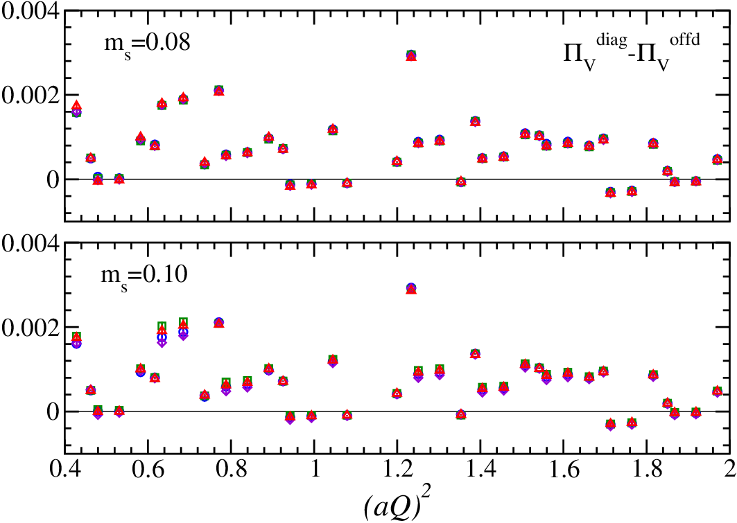
The contribution of may also be estimated by looking at a difference between VPFs obtained with (diag) and with (offd) components, i.e.
| (15) | |||||
| (16) |
respectively. Figure 6 shows as a function of . The maximum magnitude of the difference in the range is 0.003, which is the same order as the estimate from .
Adding or subtracting this amount of systematic effect from the lattice data, we repeat the whole analysis to estimate the systematic error due to the Lorentz (or WT) violating terms, which gives in .
IV.4 Quark condensate and
The uncertainty due to the quark condensate is estimated as for by varying the input value from to , which correspond to the lower and upper limits of the estimate of in [23].
The uncertainty due to is also estimated as for by varying within its estimated error (from 0.777 to 0.832).
IV.5 Perturbative expansion
The truncation effect of the perturbative expansion can be estimated by comparing the results with different orders of the perturbative expansion. Fortunately, the four-loop calculation is known for [28, 29], and we can explicitly estimate the effect of .

A comparison of two-, three- and four-loop calculations of is shown in Figure 7. They correspond to , , and calculations, respectively. We observe that the difference between three-loop and four-loop is of order of 0.0001 for , which is much smaller than other systematic effect.
Strictly speaking, the smallness of the four-loop contribution does not guarantee that the unknown higher orders are even smaller. We therefore attempted to fit the data with a formula including unknown term . The fit gives with a shift of resulting by . We therefore put a conservative systematic error from the truncation of the perturbation series as . This can only be reduced by including the data at higher values, which needs finer lattice spacings.
IV.6 expansion
As previously discussed, the size of neglected terms in the OPE formula is at most 0.001 for at the lower end of the fitting range (see Figure 4). This is less than 1/5 of the estimated discretization effect discussed above. We therefore expect that the impact on is smaller than 0.0001.
IV.7 Charm and bottom quark mass
The uncertainty of charm and bottom quark masses, and used in a perturbative matching of onto is and , which are the maximum and minimum values when are changed within in the analysis. The input values = 1.27() GeV and = 4.20() GeV are taken from [2].
IV.8 Lattice spacing
The uncertainty of the lattice spacing is the largest source of the systematic error.
Our main result is quoted with the Sommer scale = 0.49 fm as an input, with which we obtain = 1.83(1) GeV. This quantity is convenient because its numerical calculation is very precise and also because its sea quark mass dependence is mild. On the other hand, does not have a direct relation to any physical observables and one has to resort to some model to fix the central value. For this reason, one prefers other physical quantities to set the scale.
One possible candidate is the pion decay constant , which is also precisely measurable on the lattice at unphysical values of sea quark masses. The problem for this quantity is that it may have rather non-trivial sea quark mass dependence as predicted by Chiral Perturbation Theory (ChPT). Using the next-to-next-to-leading order formula in ChPT, we obtain = 1.97(4) GeV [30]. In this analysis we observed a rather large dependence on the sea quark mass and more importantly a strong curvature that bends the extrapolation to the lower value of , thus the higher value of . We therefore need more careful analysis on possible systematic errors in this determination.
One of the most popular quantities to set the scale in recent lattice calculations is the baryon mass. Since the baryon is made of three strange quarks, the dependence on up and down quark masses only comes from quark loop effect, which is expected to be small. A possible problem is that its determination has to be combined with the strange quark mass determination, which is non-trivial. In addition, the finite volume effect could be more important for baryons. Our result is = 1.76(8)() GeV, with the second error being our estimate of the finite volume effect, that is set by calculations on a larger volume lattice () but at limited values of sea quark mass.
Since each determination has its own advantage and disadvantage, we decided to take as our central value and others ( and ) to estimate the systematic uncertainties. The shift of due to the choice of and is and , respectively, which we quote as the systematic error from the scale setting.
This uncertainty also affects the matching points and , which is included in the above error band.
IV.9 Final result
| Sources | Estimated error in |
|---|---|
| Uncorrelated fit | 0.0003 |
| Lattice artifact ( effect) | 0.0003 |
| 0.0002 | |
| Quark condensate | 0.0001 |
| 0.0001 | |
| Perturbative expansion | 0.0003 |
| expansion | 0.0001 |
| Lattice spacing | |
| Total (in quadrature) |
Table 1 shows a summary of our estimate of the systematic errors in our determination of . We quote final result of the strong coupling constant at the boson mass scale as
| (17) |
Here, the first error is statistical error and the second is a sum of the various systematic errors in quadrature.
V Conclusions
Determination of the strong coupling constant may be achieved through a perturbative expansion of any physical quantity in terms of at a given scale . Experimental determination typically uses a perturbative amplitude of quarks at high energy. Comparison with the lattice QCD calculation provides a highly non-trivial test of QCD, as lattice uses low-energy hadron spectrum or matrix elements to set the scale.
In the lattice calculation, there are variety of choices for the quantity to be expanded in . In order to achieve good enough accuracy, the perturbative expansion must be known to higher orders or evaluated at very high energies. The latter may be achieved by calculating the scaling towards the high energy regime non-perturbatively using the so-called step-scaling technique (see, e.g. [5, 33]). The former is numerically less intensive but requires analytic perturbative calculations beyond one-loop level.
This work demonstrates that the vacuum polarization function can be used for the precise determination of . The important points are (i) the perturbative expansion can be done in the continuum theory and is known to , and (ii) the non-perturbative lattice calculation with controlled systematic errors is possible. The discretization error was a concern as the large points have to be calculated, but it turned out to be under control with currently available lattice setups by careful estimates of systematic effects.
The use of the overlap fermion is certainly desirable as the massless limit of quarks is uniquely defined and the use of the continuum OPE is justified. With the lattice fermions that violates chiral symmetry, one expects dangerous terms such as , whose numerical impact has to be carefully studied.
Extension of this work is straightforward. Since the largest uncertainty comes from the scale determination, a consistent determination of the lattice scale with various low-energy inputs is necessary in order to significantly improve the accuracy. This requires extensive simulations at larger volumes, smaller quark masses and smaller lattice spacings. The discretization effect in VPF considered in this work will also be significantly reduced by going to finer lattice that will become available within a few years.
Acknowledgements.
E.S. thanks Y. Kikukawa for correspondence and discussion. The work of HF was supported by the Global COE program of Nagoya University called “QFPU” from JSPS and MEXT of Japan. Numerical calculations are performed on IBM System Blue Gene Solution and Hitachi SR11000 at High Energy Accelerator Research Organization (KEK) under a support of its Large Scale Simulation Program (No. 07-16). This work is supported by the Grant-in-Aid of the Japanese Ministry of Education (No. 18740167, 19540286, 19740121, 20105005, 20340047, 20105001, 20105002, 20105003, 20025010, 21105508, 21674002, 21684013).References
- [1] S. Bethke, Eur. Phys. J. C 64, 689 (2009).
- [2] C. Amsler et al. [Particle Data Group], Phys. Lett. B 667, 1 (2008).
- [3] M. Davier, A. Hocker and Z. Zhang, Rev. Mod. Phys. 78, 1043 (2006); [arXiv:hep-ph/0507078].
- [4] E. Shintani et al. [JLQCD Collaboration and TWQCD Collaboration], Phys. Rev. D 79, 074510 (2009) [arXiv:0807.0556 [hep-lat]].
- [5] M. Della Morte, R. Frezzotti, J. Heitger, J. Rolf, R. Sommer and U. Wolff [ALPHA Collaboration], Nucl. Phys. B 713, 378 (2005); [arXiv:hep-lat/0411025].
- [6] M. Gockeler, R. Horsley, A. C. Irving, D. Pleiter, P. E. L. Rakow, G. Schierholz and H. Stuben, Phys. Rev. D 73, 014513 (2006).
- [7] S. Aoki et al. [JLQCD Collaboration], Phys. Rev. D 78, 014508 (2008) [arXiv:0803.3197 [hep-lat]].
- [8] T. W. Chiu, T. H. Hsieh, C. H.Huang and T. R. Huang, Phys. Rev. D 66, 114502 (2002).
- [9] I. Allison et al., Phys. Rev. D 78, 054513 (2008).
- [10] Y. Kikukawa and A. Yamada, Nucl. Phys. B 547, 413 (1999) [arXiv:hep-lat/9808026].
- [11] H. Neuberger, Phys. Lett. B 417, 141 (1998) [arXiv:hep-lat/9707022].
- [12] H. Neuberger, Phys. Lett. B 427, 353 (1998) [arXiv:hep-lat/9801031].
- [13] S. Hashimoto, arXiv:0811.1257 [hep-lat].
- [14] S. Aoki, H. Fukaya, S. Hashimoto and T. Onogi, Phys. Rev. D 76, 054508 (2007) [arXiv:0707.0396 [hep-lat]].
- [15] J. Noaki et al., arXiv:0907.2751 [hep-lat].
- [16] L. R. Surguladze and M. A. Samuel, Phys. Rev. Lett. 66, 560 (1991) [Erratum-ibid. 66, 2416 (1991)].
- [17] S. G. Gorishnii, A. L. Kataev and S. A. Larin, Phys. Lett. B 259, 144 (1991).
- [18] K. G. Chetyrkin, J. H. Kühn and M. Steinhauser, Nucl. Phys. B 482, 213 (1996).
- [19] K. G. Chetyrkin, A. Kwiatkowski, Z. Phys. C 59, 525 (1993).
- [20] K. G. Chetyrkin, V. P. Spiridonov and S. G. Gorishnii, Phys. Lett. B 160, 149 (1985).
- [21] G. Martinelli and C. T. Sachrajda, Nucl. Phys. B 478, 660 (1996); [arXiv:hep-ph/9605336].
- [22] J. Noaki et al. [JLQCD and TWQCD Collaborations], Phys. Rev. Lett. 101, 202004 (2008); [arXiv:0806.0894 [hep-lat]].
- [23] H. Fukaya et al. [JLQCD collaboration], arXiv:0911.5555 [hep-lat].
- [24] T. van Ritbergen, J. A. M. Vermaseren and S. A. Larin, Phys. Lett. B 400, 379 (1997)
- [25] M. Czakon, Nucl. Phys. B 710 (2005) 485 [arXiv:hep-ph/0411261].
- [26] J. Gasser and H. Leutwyler, Nucl. Phys. B 250, 465 (1985).
- [27] M. Jamin, Phys. Lett. B 538, 71 (2002).
- [28] K. G. Chetyrkin, J. H. Kühn and C. Sturm, Eur. Phys. J. C48, 107 (2006).
- [29] R. Boughezal, M. Czakon and T. Schutzmeier, Phys. Rev. D 74 (2006) 074006 [arXiv:hep-ph/0605023].
- [30] J. Noaki et al. [JLQCD and TWQCD Collaborations], PoS LAT2009, 096 (2009) [arXiv:0910.5532 [hep-lat]].
- [31] C. T. H. Davies, K. Hornbostel, I. D. Kendall, G. P. Lepage, C. McNeile, J. Shigemitsu and H. Trottier [HPQCD Collaboration], Phys. Rev. D 78, 114507 (2008) [arXiv:0807.1687 [hep-lat]].
- [32] K. Maltman, D. Leinweber, P. Moran and A. Sternbeck, Phys. Rev. D 78, 114504 (2008) [arXiv:0807.2020 [hep-lat]].
- [33] S. Aoki et al. [PACS-CS Collaboration], JHEP 0910, 053 (2009) [arXiv:0906.3906 [hep-lat]].