The first constraint that should be considered is that the total relic density of cold dark matter must match the observed value. We will consider the situation where only the LSP and the NLSP are relevant; that is, heavier MSSM particles have already decayed to LSP/NLSP before BBN takes place. In general, the final abundance of the LSP will have two components. The first one is the thermal abundance, $\Omega^{\rm TP}_{\rm LSP}$, which comes from thermal processes occurring in the plasma like scatterings and freeze-out. The second one is the non-thermal component, $\Omega^{\rm NTP}_{\rm LSP}$, that includes the contribution from LSP particles produced in NLSP decay. Therefore, the total cold dark matter relic density, will be ³³ 3 Recall that we are assuming that the NLSP lifetime is smaller than the age of the Universe. If it were not the case, Eq. (2) is still valid as we are considering $m_{\rm NLSP}\simeq m_{\rm LSP}$.

where the last term stands for $\Omega^{\rm NTP}_{\rm LSP}$ and we have used Eq. (1). Assuming no late entropy release, Eq. (2) represents the present amount of dark matter, which should be equated with the observed value [5]

It is useful to define the new parameter

which quantifies the amount of present cold dark matter coming from the NLSP decay. In this equation $Y_{{\rm NLSP}}$ refers to the NLSP yield just before its decay ⁴⁴ 4 Here the yield of a species $i$ is defined as the ratio of the number density $n_{i}$ to entropy, $Y_{i}\equiv n_{i}/s$. Recall also that the yield and the relic density of a massive particle species $i$ are related through $Y_{i}\simeq 4.1\times 10^{-12}\left(100\,\mbox{GeV}/m_{i}\right)\left(\Omega_{i}\,h^{2}/0.11\right)$.. Combining Eq. (2) and Eq. (4) we get that

which implies that $\omega\leq 1$ independently of $\delta$.

At temperatures of order $T\sim 1$ MeV, the light nuclei are synthesized in the primordial plasma. These temperatures corresponds to times between 1 sec and $10^{3}$ sec. The obtained abundances in standard BBN calculations are in striking agreement with observation ⁵⁵ 5 There are possible discrepancies in Lithium abundances, which might be explained using Gravitino dark matter  [6, 7]. . However, the injection of energetic particles in the primordial plasma at BBN or later can disrupt the standard BBN processes [8, 9, 10, 11], leading to a disagreement between theory and observation. Thus, any additional particle decaying at BBN or later is subject to the strong constraints from light nuclei abundances. Usually, the energy of injected particles is assumed to be of the same order of the LSP/NLSP mass and stringent bounds were derived for various scenarios from BBN [12, 13, 14, 15, 16, 17, 18, 19, 20, 21]. These constraints are obtained by solving the full set of Boltzmann equations for BBN with a late-decaying particle. This requires the detailed study of the spectrum of decay products with all the relevant nuclear cross sections [9, 10, 11]. The constraints apply to the released electromagnetic or hadronic energy, parametrised by $\xi_{i}$ defined as [13]

where $E_{i}$ is the released energy per decay with $i=$ em for electromagnetic decays and $i=$ had for the hadronic ones and $B_{i}$ stands for the respective branching ratios. The constraints from hadronic processes are important when the lifetime is relatively short $\tau_{\rm NLSP}\lesssim 10^{7}$ sec [10, 16]. The typical lifetimes considered in this work are larger that $10^{7}$ sec and therefore, in the following, we will consider only the BBN constraints on $\xi_{\rm em}$.

In the 2-body electromagnetic decay, the corresponding released energy is

where we assumed that the visible particle mass is negligible. In the degenerate mass limit, $\delta\ll 1$, this reduces to $E_{\rm em}\simeq m_{{\rm LSP}}\,\delta$. Notice that, as emphasized before, $E_{\rm em}$ is much smaller than the usually⁶⁶ 6 Small mass differences has been considered in [21, 22] and for completely different motivations than ours. assumed value $m_{{\rm NLSP}}/2$.

Given the above discussion, for our purposes, we can apply the constraints on $\xi_{\rm em}$ from Ref. [11] directly to our scenario. Then, the constraint on $\xi_{\rm em}$ reads

where the right hand side in the above equation can be read off from the upper limit derived in [11] for $B_{\rm had}=0$.

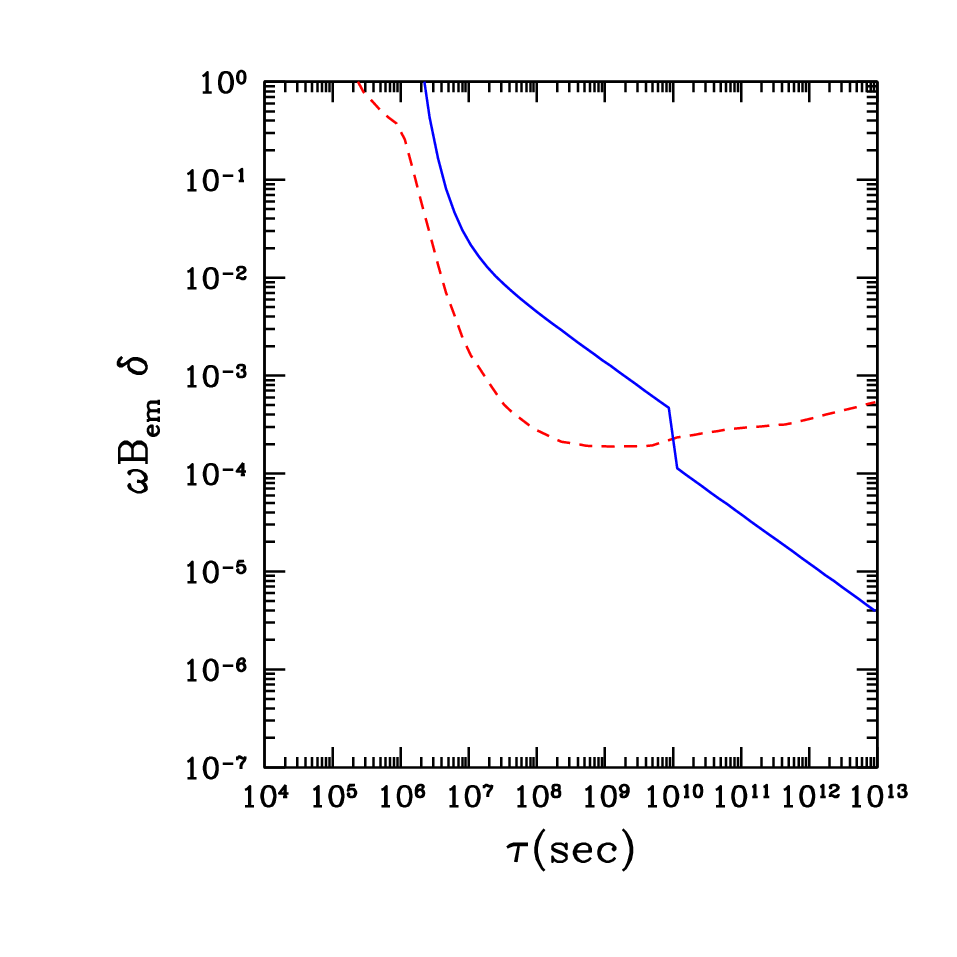
For general values, the upper limit on the product $\omega\,B_{\rm em}\,\delta$ from BBN is shown in Figure 1 with red (dashed) line. From this figure, we can see that for lifetimes between $10^{7}$ and $10^{10}$ sec, this constraint requires $\omega B_{\rm em}\delta$ to be between $10^{-3}$ and $10^{-4}$. Notice that BBN constraints apply equally to the case of charged NLSP decaying to gravitino and electromagnetic showers.

In addition to BBN constrains, for long lifetimes $\tau_{\rm NLSP}\mathrel{\hbox to0.0pt{\lower 4.0pt\hbox{\hskip 1.0pt$\sim$}\hss}\raise 1.0pt\hbox{$>$}}10^{7}$ sec., there are strong bounds from the shape of the CMB black-body spectrum. As pointed out in [12], the late injection of electromagnetic energy may distort the frequency dependence of the CMB spectrum from its observed blackbody shape. At late times of interest in our scenario, energetic photons from NLSP decays lose energy through processes such as $\gamma e^{-}\rightarrow\gamma e^{-}$, but photon number remains conserved since other processes, like double Compton scatterings and thermal bremsstrahlung, become inefficient. As a result, the spectrum follows the Bose–Einstein distribution function

where $\mu$ here denotes the chemical potential. Then, the chemical potential of the distorted CMB spectrum has to satisfy the constraint, $|\mu|<9\times 10^{-5}$ [23], which, for decay lifetimes $\tau_{{\rm NLSP}}\mathrel{\hbox to0.0pt{\lower 4.0pt\hbox{\hskip 1.0pt$\sim$}\hss}\raise 1.0pt\hbox{$<$}}8.8\times 10^{9}\sec$, translates into an upper bound on the released energy from NLSP decay, $\xi_{\rm em}$ defined in Eq. (6) [24, 15],

where $\tau_{dC}\simeq 6.085\times 10^{6}$ sec.

For longer lifetimes ($\tau_{{\rm NLSP}}\mathrel{\hbox to0.0pt{\lower 4.0pt\hbox{\hskip 1.0pt$\sim$}\hss}\raise 1.0pt\hbox{$>$}}8.8\times 10^{9}\sec$), the spectral distortions in the CMB spectrum can be described in terms of the integral of the fractional contributions to the energy $\epsilon$ of the CMB per comoving volume during decay through the Compton $y$ parameter, $4y=\delta\epsilon/\epsilon$, given by

where $T(t)$ is the CMB temperature and $t_{\rm eff}=[\Gamma(1-\beta)]^{1/\beta}\tau_{{\rm NLSP}}$, for a time–temperature relation $T\propto t^{-\beta}$, with $\Gamma$ the usual Gamma function. In the radiation dominated era in the early Universe, for $T<0.1\,\mbox{MeV}$,

which gives $\beta=1/2$. Thus $t_{eff}=[\Gamma(1/2)]^{2}\tau_{{\rm NLSP}}=\pi\tau_{{\rm NLSP}}$.

The observational limit $|y|<1.2\times 10^{-5}$ [25] gives the constraint

Using Eqs. (11,13), this CMB constraint is plotted in Figure 1 with blue (solid) line. We can see that for lifetimes $\tau_{{\rm NLSP}}\gtrsim 10^{10}$ sec. the CMB constraint becomes more stringent than the BBN ones and sets the constraint on $\xi_{\rm em}$ until recombination time. Similarly to the BBN, CMB constraints apply also to charged NLSP decaying to gravitino and electromagnetic showers.

After recombination, at the cosmic time around $10^{13}$ sec, the number density of free electrons drops quickly and the photons are almost free from the interactions. Therefore the photons from the decaying particles can reach us now and contribute to the Cosmic Gamma-ray Background (CGB). The observed CGB highly constrains any extra contribution including the photons from late decaying particles ⁷⁷ 7 Under appropriate conditions, the late decays of WIMPs to gravitinos and MeV photons may explain the MeV CGB anomalies [22]..

The present photon flux from two-body decay can be written as

where $E_{\rm em}\simeq m_{{\rm LSP}}\delta$ is the energy of the photon at production, $\tau_{{\rm NLSP}}$ and $m_{{\rm NLSP}}$ are the lifetime and mass of NLSP, $\rho_{c}=3H_{0}^{2}/8\pi G_{N}=8.0992h^{2}\times 10^{-47}\,\mbox{GeV}^{4}$ and $a=a(t)$ is the time-dependent scale factor with $a(t_{0})=1$ at present time $t_{0}$. The delta function can be integrated using the formula $\delta(f(t))=\delta(t-t_{a})/|f^{\prime}(t=t_{a})|$ where $t_{a}$ is the solution which satisfies $E_{\gamma}=a(t_{a})E_{\rm em}$. After integration, the flux reads

where the $\Theta$ function simply cuts energies larger than the initial energy and each observed photon with energy $E_{\gamma}$ is produced at a time $t_{a}$ which satisfies $a(t_{a})=E_{\gamma}/E_{\rm em}$. Assuming the dark energy is a cosmological constant, this function $t_{a}(a)$ is given by [22]

where $H(a)=H_{0}\sqrt{\Omega_{M}a^{-3}+\Omega_{\Lambda}}$.

Taking into account that $c/H_{0}=1.3\times 10^{28}\,\mbox{cm}$, $\rho_{c}=5.6\times 10^{-6}\,\mbox{GeV}/\,\mbox{cm}^{3}$, $H_{0}=70\,\mbox{km}\,\sec^{-1}\,\,\mbox{Mpc}^{-1}$, $\Omega_{\Lambda}=0.7$, $\Omega_{M}=\Omega_{\rm CDM}+\Omega_{B}=0.3$ and $\Omega_{\rm CDM}=\Omega_{\rm WMAP}=0.25$, we find that the flux is

with

This differential flux must be compared to the observation of diffuse gamma ray flux. At each photon energy, we must require that this flux is smaller than the flux, $E_{\gamma}^{2}\frac{d\Phi}{dE_{\gamma}}$, observed by SPI, COMPTEL and EGRET [3]. Notice that, unlike the BBN and CMB constraints where we can find a bound on $\xi_{\rm em}$ for a given value of $\tau_{{\rm NLSP}}$, now we need to specify both $\tau_{{\rm NLSP}}$ and $E_{\gamma}$ to obtain a bound on $\omega B_{\rm em}\delta$.

On the other hand, if the lifetime of NLSP is longer than the age of Universe, the line spectrum from the galactic center can be observed without cosmological redshift and this provides a further constraint on the emitted radiation from NLSP decays. For this we apply the bounds from Ref. [3]. Taking into account of the exponential decay of NLSP we have

where $\rho_{sc}=0.3\,\mbox{GeV}\,\mbox{cm}^{-3}$ is the dark matter density at the solar distance from the Galactic center, $R_{sc}=8.5\,\mbox{kpc}$, $\zeta_{lim}$ is a dimensionless integral of the line-of-sight intensity in the galactic center which ranges between $0.5-1.5$ for various dark matter halo profiles [3]. The function $\mathcal{F}$ is given in Figure 2 of Ref. [3]. Once again, as in the case of the CGB constraint in Eq. (17), this constraint depends on the photon energy and therefore we need to specify both $\tau_{{\rm NLSP}}$ and $E_{\gamma}$ to obtain bound on $\omega B_{\rm em}\delta$. Thus, there is no simple analog of Figure 1 for a constraint on $\xi_{\rm em}$ from Diffuse gamma rays observations. Moreover, the constraints on $\xi_{\rm em}$ from the galactic center gamma rays are of the same order of magnitude (although slightly stronger) as the ones from the diffuse extragalactic emission. Therefore, for simplicity, we will only consider the diffuse gamma rays constraints, which apply to a broader range of energy.

Heavy long-lived negatively charged particles, $X^{-}$, present during BBN can bind with light nuclei modifying standard BBN reactions. These catalyzed reactions, called CBBN, result in a change of light element abundances, and in particular lead to the overproduction of ${}^{6}\textrm{Li}$ through CBBN reactions  [26]. For lifetimes longer than $5\times 10^{3}\sec$, the observed light-nuclei abundances result on a constraint on the abundance of the charged relic, $Y_{X^{-}}<2\times 10^{-16}$ [27, 28]. However, taking more conservative ${}^{6}\textrm{Li}/^{7}\textrm{Li}$ constraints, it is possible to relax slightly the previous bound to $Y_{X^{-}}<10^{-14}$–$10^{-15}$  [29, 30].

Using Eq. (4), we can translate the constraint on the yield of charged NLSP from catalyzed BBN to a bound on $\omega$

where we used $\Omega_{\rm WMAP}h^{2}=0.11$ and $Y_{\textrm{CBBN}}$ is the maximum value allowed from catalyzed BBN for lifetimes larger than $10^{5}\sec$. As can be see from this equation, the catalyzed BBN bound is very stringent and indeed, it is very difficult to obtain such small yield at freeze-out in the MSSM [31]. However, it is still possible to find small allowed regions in the MSSM, or even in the CMSSM, where the ${\widetilde{\tau}}$ is the NLSP with large $\tan\beta$ [32, 33] with relaxed ${}^{6}\textrm{Li}/^{7}\textrm{Li}$ bounds [21].

As usual, in the MSSM, the lightest neutralino eigenstate $\chi^{0}_{1}$ is parametrised as $\chi^{0}_{i}=N_{i1}(-i\widetilde{B})+N_{i2}(-i\widetilde{W}_{3})+N_{i3}\widetilde{H}^{0}_{U}+N_{i4}\widetilde{H}^{0}_{D}$, where the unitary matrix $N$ defines the composition of neutralinos in terms of the Bino, Wino and Higgsinos. Since we are considering mass splittings that are smaller than the $Z$ mass to suppress the hadronic branching ratio, the dominant (2-body) decay channel will be $\chi^{0}_{1}\to\gamma\,\widetilde{G}$ or $\widetilde{G}\to\chi^{0}_{1}\gamma$. As we will see below, the typical lifetime of NLSP is of order $10^{13}\sec\times\left(1\,\mbox{GeV}/\Delta M\right)^{3}$. Therefore, depending on $\Delta M$ we will have to consider different constraints.

In the MSSM, the lightest stau state ${\widetilde{\tau}}_{1}$ can also be the LSP. However this situation is usually discarded as staus cannot play the role of cold dark matter. The remaining possibility is then that ${\widetilde{\tau}}_{1}$ is the NLSP with the gravitino as the LSP. The dominant decay channel in this case is ${\widetilde{\tau}}_{1}\to\tau\,\widetilde{G}$ if the mass-difference is larger than the tau mass, i.e. $\Delta M\geq 1.77\,\mbox{GeV}$  ¹²¹² 12 Notice that for $\Delta M\leq 1.77\,\mbox{GeV}$ the two body flavour-conserving channel is closed and the stau can decay only through lepton flavour violating channels, ${\widetilde{\tau}}_{1}\to\mu\,\widetilde{G}$ or ${\widetilde{\tau}}_{1}\to e\,\widetilde{G}$, where the lifetime would be inversely proportional to the lepton-flavour violating coupling [42, 43]: $\tau_{{\widetilde{\tau}}_{1}}\simeq 2\times 10^{14}\sec|\delta^{\rm LFV}_{\tau i}|^{-2}$ for $m_{3/2}=100\,\mbox{GeV}$ and $\Delta M=2\,\mbox{GeV}$. This means that, if these flavour violating couplings, the so-called Mass Insertions, are sizable, $\delta^{\rm LFV}_{\tau i}\geq 0.03$, the stau could decay before the present time. However, we do not consider this possibility in this paper. . In this case, the lifetime of the stau NLSP is then given by

Notice that now, the stau lifetime, in contrast with the degenerate gravitino-neutralino case, does depend on the overall mass scale $m_{3/2}$. Moreover for a mass difference similar to the tau mass, $\Delta M\simeq 1.78\,\mbox{GeV}$, the stau lifetime is equal to the age of the universe.

In principle, the stau has to satisfy similar constraints as in the degenerate gravitino-neutralino case with the exception of diffuse gamma ray constraints. Notice that the stau does not decay directly to photons and therefore does not contribute to the gamma ray background. Despite this fact, all the decays of the stau produce electromagnetic cascades that affect both BBN and CMB observables.

Nevertheless, the main difference with the neutralino case is that stau, being charged, can form bound states with light elements and affect BBN predictions [28, 29]. Then, from Eq. (20) we obtain a strong constraint on $\omega$ which for $Y_{\rm CBBN}=10^{-15}$ is $\omega<7.32\times 10^{-4}m_{\widetilde{\tau}}/(300{\rm GeV})$.

Finally, if the stau lifetime is longer than the age of the universe, the stau yield is very strongly bounded by the presence of anomalously heavy Hydrogen in deep sea water [44]. In terms of $\omega$ the bound reads, $\omega\leq 2.2\times 10^{-27}\left(m_{{\widetilde{\tau}}}/100\,\mbox{GeV}\right)$, for stau masses between 5 GeV and 1.7 TeV. Thus, in practice, this possibility can be completely discarded. In our analysis, we require that staus have already decayed at present and therefore we eliminate the staus with a lifetime longer than the age of the universe which corresponds to $\Delta M\lesssim 2\,\mbox{GeV}$.

These constraints are presented in Figure 4 where we see that for $Y_{\rm CBBN}=10^{-15}$ the CBBN is the most stringent of all the constraints and requires $\omega\lesssim 7\times 10^{-4}$. This corresponds to stau relic density well below the observed relic density, Eq. (3), and the thermal relic density at freeze-out for purely RH staus [31]. In order to get such small abundance, the staus must have a substantial LR mixing. This requires both large $\mu$ and large $\tan\beta$ and moderate $m_{{\widetilde{\tau}}_{1}}$ [32, 33], which as we will see in section 4, is difficult, but still possible in the CMSSM. Furthermore, the vertical line at $\Delta M\simeq 2\,\mbox{GeV}$ corresponds to our requirement that all staus have already decayed at the present age.

The bound on $T_{\rm RH}$ here is analogous to the case of gravitino-neutralino degeneracy with gravitino LSP. Again, the reheating temperature is given in Eq. (24) and given that, in this case, the allowed points in parameter space require $\omega\lesssim 10^{-2}$, one gets the maximal reheating temperature $T_{\rm RH}=4.1\times 10^{9}$ GeV.

In Fig. 5 we show the region of ${\rm w}\leq 1$ (corresponding to $\Omega_{\chi}h^{2}\leq 0.115$) in the ($m_{1/2}$, $m_{0}$) plane for $A_{0}=0$, $\tan\beta=10$, whereas we have chosen $\mu>0$ motivated by $(g-2)_{\mu}$ data. In the CMSSM, the only mechanism which provides a dark matter abundance consistent with the WMAP value, if we require agreement with $(g-2)_{\mu}$ at 3 $\sigma$, is stau-neutralino coannihilations [63]. This region is located in a narrow band above the stau-neutralino degeneracy line ($m_{{\widetilde{\tau}}}=m_{\chi}$). In addition to this relic abundance constraint, the only effective constraint in this region comes from direct Higgs searches at LEP which excludes low gaugino masses $m_{1/2}\lesssim 300\,\mbox{GeV}$. In this figure, the allowed values for ${\rm w}$ are shown in different colours. As we can see, in this case, we can only obtain ${\rm w}$ between 1 and $\mathcal{O}(10^{-1})$. In the region of $m_{{\widetilde{\tau}}}\leq m_{\chi}$, although the annihilation mechanisms are more efficient than in the neutralino case due to fact that the stau is a charged particle, the lowest ${\rm w}$ we can reach is ${\rm w}_{\min}\sim 7\times 10^{-2}$, whereas from Eq. (20) we see that the most conservative bound $Y_{\widetilde{\tau}}<10^{-14}$ from catalyzed nuclear reactions would require ${\rm w}\lesssim 2.7\times 10^{-3}$. Hence, this region of $m_{{\widetilde{\tau}}}\leq m_{\chi}$ is completely excluded for all values of $\Delta M$. If we eliminate the requirement of a non-zero SUSY contribution to $(g-2)_{\mu}$, we obtain two small regions. First, there is a vertical strip at high $m_{0}$ corresponding to a pole in the annihilation $\chi\chi\to b\bar{b}$ via the lightest Higgs. In this region we can obtain values of ${\rm w}$ as low as ${\rm w}\simeq 0.01$. Then, there is a long strip, below the non-electroweak symmetry breaking (NEWB) region, at very large $m_{0}$, where the neutralino is a mixed Bino-Higgsino state and the annihilation to $W^{+}W^{-}$ is efficient enough to get a right relic abundance. However, in this region we obtain always ${\rm w}\gtrsim 0.1$.

Using these allowed values for w and the corresponding $\omega$ values, we obtain a bound on the mass difference $\Delta M$ in our degenerate gravitino scenario from Figure 2. According to Figure 2, for $\omega\geq 0.03$ the relevant constraint is diffuse gamma ray observations, and this requires $\Delta M\leq 10^{-2}$ GeV. This means that the lifetime of the NLSP (neutralino or gravitino) is longer than the age of the universe. Notice that, in the case of gravitino LSP, the fact that we cannot obtain w $=\omega<0.1$ implies that this scenario would be completely ruled out by BBN, CMB and diffuse gamma ray observations, unless $\Delta M<10^{-2}$ GeV and the neutralinos are beginning to decay at present. However, if the gravitino is the NLSP, we have two possibilities. The first possibility would be that the observed dark matter abundance is provided completely by the neutralino w $\simeq 1$, with only a small fraction, at the level of $10^{-3}$, due to gravitinos. This corresponds to $T_{\rm RH}$ of the order of $10^{7}$ GeV, which is the usual situation in previous studies. The second possibility would be that there is a sizeable fraction of the dark matter due to gravitinos but, again, this would require $\Delta M<10^{-2}$ GeV corresponding to a very long gravitino lifetime which permits to evade the cosmological bounds. The maximum values of $T_{\rm RH}$ in these scenarios are shown in Fig. 6. As it can be seen from this figure, values of $T_{\rm RH}>10^{9}\,\mbox{GeV}$ consistent with thermal leptogenesis are accessible in the model, although this is only possible if $\Delta M\leq 10^{-2}$ GeV.

In Fig. 7, we analyze the case of $\tan\beta=50$. For large values of $\tan\beta$, in the neutralino MSSM LSP region ($m_{\chi}\leq m_{{\widetilde{\tau}}}$), we have different mechanisms to get a correct relic density consistent with WMAP. These mechanisms are i) stau-neutralino coannihilations, ii) “A-pole” region, where the s-channel exchange of the CP-odd Higgs boson, $A$, can become nearly resonant [64, 65] and iii) the “focus point” or “hyperbolical branch” where a significant higgsino component, enhances its annihilation cross sections into final states containing gauge and/or Higgs bosons [66, 67, 68]. In fact, the focus point region occurs at $m_{0}$ much larger than $m_{1/2}$ and therefore multi-TeV scalar masses which implies that $\delta a_{\mu}^{MSSM}$ is well below the lower $2\sigma$ limit due to SUSY decoupling [69]. However, if we accept $\delta a_{\mu}^{MSSM}$ at the $3\sigma$ level we can also reach the “focus point” region for $m_{0}\simeq 2\times 10^{3}\,\mbox{GeV}$. Both the neutralino-stau coannihilation band and the “A-pole” region merge for $\tan\beta=50$ as we can see in this figure. This region is cut from the small $m_{1/2}$ values by the lower $2\sigma$ limit of the $BR(\overline{B}\rightarrow X_{s}\gamma)$ constraint ¹⁵¹⁵ 15 The reason for this is the destructive interference of the chargino/squark loops which grows with $\tan\beta$ [70]. This effect is enhanced for chargino masses $\leq 100\,\,\mbox{GeV}$ whereas is never dramatic for masses around $1$ TeV or larger.. This constraint limits the minimum possible value of w obtainable through the “A-pole”. Therefore we can only reach ${\rm w}_{\min}\sim 0.1$ both in the coannihilation and “A-pole” regions. In the “focus point” region the situation is again similar and we can reach only values ${\rm w}_{\min}\sim 0.1$–$0.01$.

In the case of $m_{{\widetilde{\tau}}}\leq m_{\chi}$, we can observe an allowed narrow band close to the tachyonic region in which the staus annihilate to $b\bar{b}$ via a pole in the s-channel exchanging a lightest Higgs. This process allows for values of ${\rm w}_{\min}\sim 10^{-5}$ which are consistent with the conservative CBBN constraint, $Y_{\widetilde{\tau}}<10^{-14}$–$10^{-15}$. The broader band at large $m_{1/2}$ corresponds to the annihilation into a pair of light Higgses exchanging a light Higgs via a s-channel and here we obtain ${\rm w}_{\min}\sim 10^{-3}$ and therefore $Y_{\widetilde{\tau}}<10^{-14}$. On the other hand, we have to keep in mind that if we had imposed the more severe constraint $Y_{\widetilde{\tau}}<10^{-16}$, both regions would be ruled out.

Likewise, with these values for w, we obtain, from Figure 2, the allowed values for the mass difference $\Delta M$. In the neutralino-stau coannihilation or A-pole regions only $\Delta M\leq 10^{-2}$ GeV are allowed, similarly to the $\tan\beta=10$ case. However, in the region of $m_{{\widetilde{\tau}}}\leq m_{\chi}$ with values of w $\gtrsim 10^{-5}$, we can see from Fig. 4 that values of the mass difference, $90\,\mbox{GeV}>\Delta M\gtrsim 1$ GeV, would be still allowed for these points ¹⁶¹⁶ 16 We are considering only $\Delta M<90\,\mbox{GeV}$ where the hadronic BBN constraints are not efficient..

The maximum values of $T_{\rm RH}$ are shown in Fig. 8. As we have seen before, both for the gravitino LSP and gravitino NLSP cases $T_{\rm RH}\propto(1-{\rm w})$. The Maximal reheating temperatures for $m_{\chi}<m_{\widetilde{\tau}}$ are always $T_{\rm RH}>10^{9}\,\mbox{GeV}$ if the condition of $\Delta M\lesssim 10^{-2}$ GeV is satisfied, as in the case of $\tan\beta=10$. However, the region below the stau–neutralino degeneracy line are only allowed in the case of gravitino LSP when the maximal reheating temperatures are again $T_{\rm RH}>10^{9}\,\mbox{GeV}$, although in this case we do not require a tight degeneracy between gravitino and stau.

In Fig. 9, the case of $\tan\beta=55$ is explored. Similarly to the case of $\tan\beta=50$, in the neutralino MSSM LSP region, the main annihilation mechanisms are the neutralino-stau coannihilation and the “A-pole” resonance, however the “focus point” region is absent in this case. Again the $BR(\overline{B}\rightarrow X_{s}\gamma)$ constraint limits the minimum possible value of w obtainable through the “A-pole”. Therefore we can only reach ${\rm w}_{\min}\sim 0.1$, both in the coannihilation and “A-pole” regions.

In the case of $m_{{\widetilde{\tau}}}\leq m_{\chi}$, as for $\tan\beta=50$, staus annihilate through an s-channel exchange of the light Higgs to a pair of light Higgses, although the annihilation to $b\bar{b}$ is suppressed in this case (it does not satisfy the required constraint $Y_{\widetilde{\tau}}<10^{-14}$). The allowed process, ${\widetilde{\tau}}{\widetilde{\tau}}\to hh$, allows for values of ${\rm w}_{\min}\sim 6\times 10^{-4}$ which are consistent with the conservative CBBN constraint for $Y_{\widetilde{\tau}}<10^{-15}$.

Likewise, with these values of w, from Figure 2 we obtain the allowed values for the mass difference $\Delta M$. As before, in the neutralino-stau coannihilation or A-pole regions only $\Delta M\leq 10^{-2}$ GeV are allowed and in the region of $m_{{\widetilde{\tau}}}\leq m_{\chi}$ mass differences $90\,\mbox{GeV}>\Delta M>2$ GeV would be still allowed. The corresponding values of $T_{\rm RH}$ are shown in Fig. 10. The discussion of section 4.2 applies also in this case.

References

- [1] C. Picciotto and M. Pospelov, “Unstable relics as a source of galactic positrons,” Phys. Lett. B 605 (2005) 15 [arXiv:hep-ph/0402178].
- [2] D. Hooper and L. T. Wang, “Evidence for axino dark matter in the galactic bulge,” Phys. Rev. D 70 (2004) 063506 [arXiv:hep-ph/0402220].
- [3] H. Yuksel and M. D. Kistler, “Dark Matter Might Decay… Just Not Today!,” Phys. Rev. D 78 (2008) 023502 [arXiv:0711.2906 [astro-ph]].
- [4] T. Moroi, “Effects of the gravitino on the inflationary universe,” arXiv:hep-ph/9503210.
- [5] E. Komatsu et al. [WMAP Collaboration], “Five-Year Wilkinson Microwave Anisotropy Probe (WMAP) Observations:Cosmological Interpretation,” Astrophys. J. Suppl. 180, 330 (2009) [arXiv:0803.0547 [astro-ph]].
- [6] K. Jedamzik, K. Y. Choi, L. Roszkowski and R. Ruiz de Austri, “Solving the cosmic lithium problems with gravitino dark matter in the CMSSM,” JCAP 0607 (2006) 007 [arXiv:hep-ph/0512044].
- [7] S. Bailly, K. Jedamzik and G. Moultaka, “Gravitino Dark Matter and the Cosmic Lithium Abundances,” Phys. Rev. D 80 (2009) 063509 [arXiv:0812.0788 [hep-ph]].
- [8] R. H. Cyburt, J. R. Ellis, B. D. Fields and K. A. Olive, “Updated nucleosynthesis constraints on unstable relic particles,” Phys. Rev. D 67 (2003) 103521 [arXiv:astro-ph/0211258].
- [9] K. Jedamzik, “Did something decay, evaporate, or annihilate during big bang nucleosynthesis?,” Phys. Rev. D 70 (2004) 063524 [arXiv:astro-ph/0402344].
- [10] M. Kawasaki, K. Kohri and T. Moroi, “Hadronic decay of late-decaying particles and big-bang nucleosynthesis,” Phys. Lett. B 625 (2005) 7 [arXiv:astro-ph/0402490]; M. Kawasaki, K. Kohri and T. Moroi, “Big-bang nucleosynthesis and hadronic decay of long-lived massive particles,” Phys. Rev. D 71 (2005) 083502 [arXiv:astro-ph/0408426].
- [11] K. Jedamzik, “Big bang nucleosynthesis constraints on hadronically and electromagnetically decaying relic neutral particles,” Phys. Rev. D 74 (2006) 103509 [arXiv:hep-ph/0604251].
- [12] J. R. Ellis, J. E. Kim and D. V. Nanopoulos, “Cosmological Gravitino Regeneration And Decay,” Phys. Lett. B 145, 181 (1984).
- [13] J. L. Feng, S. Su and F. Takayama, “Supergravity with a gravitino LSP,” Phys. Rev. D 70 (2004) 075019 [arXiv:hep-ph/0404231].
- [14] J. R. Ellis, K. A. Olive, Y. Santoso and V. C. Spanos, “Gravitino dark matter in the CMSSM,” Phys. Lett. B 588 (2004) 7 [arXiv:hep-ph/0312262].
- [15] L. Roszkowski, R. Ruiz de Austri and K. Y. Choi, “Gravitino dark matter in the CMSSM and implications for leptogenesis and the LHC,” JHEP 0508 (2005) 080 [arXiv:hep-ph/0408227].
- [16] K. Kohri, T. Moroi and A. Yotsuyanagi, “Big-bang nucleosynthesis with unstable gravitino and upper bound on the reheating temperature,” Phys. Rev. D 73 (2006) 123511 [arXiv:hep-ph/0507245].
- [17] D. G. Cerdeno, K. Y. Choi, K. Jedamzik, L. Roszkowski and R. Ruiz de Austri, “Gravitino dark matter in the CMSSM with improved constraints from BBN,” JCAP 0606 (2006) 005 [arXiv:hep-ph/0509275].
- [18] F. D. Steffen, “Gravitino dark matter and cosmological constraints,” JCAP 0609 (2006) 001 [arXiv:hep-ph/0605306].
- [19] J. Pradler and F. D. Steffen, “Thermal Gravitino Production and Collider Tests of Leptogenesis,” Phys. Rev. D 75 (2007) 023509 [arXiv:hep-ph/0608344].
- [20] M. Kawasaki, K. Kohri, T. Moroi and A. Yotsuyanagi, “Big-Bang Nucleosynthesis and Gravitino,” Phys. Rev. D 78 (2008) 065011 [arXiv:0804.3745 [hep-ph]].
- [21] S. Bailly, K. Y. Choi, K. Jedamzik and L. Roszkowski, “A Re-analysis of Gravitino Dark Matter in the Constrained MSSM,” JHEP 0905 (2009) 103 [arXiv:0903.3974 [hep-ph]].
- [22] J. A. R. Cembranos, J. L. Feng and L. E. Strigari, “Resolving Cosmic Gamma Ray Anomalies with Dark Matter Decaying Now,” Phys. Rev. Lett. 99 (2007) 191301 [arXiv:0704.1658 [astro-ph]].
- [23] D. J. Fixsen, E. S. Cheng, J. M. Gales, J. C. Mather, R. A. Shafer and E. L. Wright, “The Cosmic Microwave Background Spectrum from the Full COBE/FIRAS Data Set,” Astrophys. J. 473 (1996) 576 [arXiv:astro-ph/9605054].
- [24] W. Hu and J. Silk, “Thermalization constraints and spectral distortions for massive unstable relic particles,” Phys. Rev. Lett. 70 (1993) 2661.
- [25] K. Hagiwara et al. [Particle Data Group], “Review of particle physics,” Phys. Rev. D 66 (2002) 010001.
- [26] M. Pospelov, “Particle physics catalysis of thermal big bang nucleosynthesis,” Phys. Rev. Lett. 98 (2007) 231301 [arXiv:hep-ph/0605215]; K. Kohri and F. Takayama, “Big Bang Nucleosynthesis with Long Lived Charged Massive Particles,” Phys. Rev. D 76 (2007) 063507 [arXiv:hep-ph/0605243]; M. Kaplinghat and A. Rajaraman, “Big Bang Nucleosynthesis with Bound States of Long-lived Charged Particles,” Phys. Rev. D 74 (2006) 103004 [arXiv:astro-ph/0606209].
- [27] K. Hamaguchi, T. Hatsuda, M. Kamimura, Y. Kino and T. T. Yanagida, “Stau-catalyzed Li-6 production in big-bang nucleosynthesis,” Phys. Lett. B 650 (2007) 268 [arXiv:hep-ph/0702274].
- [28] J. Pradler and F. D. Steffen, “Implications of Catalyzed BBN in the CMSSM with Gravitino Dark Matter,” Phys. Lett. B 666 (2008) 181 [arXiv:0710.2213 [hep-ph]].
- [29] K. Jedamzik, “Bounds on long-lived charged massive particles from Big Bang nucleosynthesis,” JCAP 0803 (2008) 008 [arXiv:0710.5153 [hep-ph]].
- [30] K. Jedamzik and M. Pospelov, “Big Bang Nucleosynthesis and Particle Dark Matter,” arXiv:0906.2087 [hep-ph].
- [31] C. F. Berger, L. Covi, S. Kraml and F. Palorini, “The number density of a charged relic,” JCAP 0810 (2008) 005 [arXiv:0807.0211 [hep-ph]].
- [32] M. Ratz, K. Schmidt-Hoberg and M. W. Winkler, “A note on the primordial abundance of stau NLSPs,” JCAP 0810 (2008) 026 [arXiv:0808.0829 [hep-ph]].
- [33] J. Pradler and F. D. Steffen, “Thermal relic abundances of long-lived staus,” Nucl. Phys. B 809 (2009) 318 [arXiv:0808.2462 [hep-ph]].
- [34] H. P. Nilles, M. Peloso and L. Sorbo, “Nonthermal production of gravitinos and inflatinos,” Phys. Rev. Lett. 87 (2001) 051302 [arXiv:hep-ph/0102264].
- [35] M. Bolz, A. Brandenburg and W. Buchmuller, “Thermal Production of Gravitinos,” Nucl. Phys. B 606 (2001) 518 [Erratum-ibid. B 790 (2008) 336] [arXiv:hep-ph/0012052].
- [36] V. S. Rychkov and A. Strumia, “Thermal production of gravitinos,” Phys. Rev. D 75 (2007) 075011 [arXiv:hep-ph/0701104].
- [37] S. Davidson and A. Ibarra, “A lower bound on the right-handed neutrino mass from leptogenesis,” Phys. Lett. B 535, 25 (2002) [arXiv:hep-ph/0202239].
- [38] G. F. Giudice, A. Notari, M. Raidal, A. Riotto and A. Strumia, “Towards a complete theory of thermal leptogenesis in the SM and MSSM,” Nucl. Phys. B 685 (2004) 89 [arXiv:hep-ph/0310123].
- [39] S. Antusch and A. M. Teixeira, “Towards constraints on the SUSY seesaw from flavour-dependent leptogenesis,” JCAP 0702 (2007) 024 [arXiv:hep-ph/0611232].
- [40] M. Olechowski, S. Pokorski, K. Turzynski and J. D. Wells, “Reheating Temperature and Gauge Mediation Models of Supersymmetry Breaking,” arXiv:0908.2502 [hep-ph].
- [41] C. Arina and N. Fornengo, “Sneutrino cold dark matter, a new analysis: Relic abundance and detection rates,” JHEP 0711 (2007) 029 [arXiv:0709.4477 [hep-ph]].
- [42] A. Masiero, S. K. Vempati and O. Vives, “Massive neutrinos and flavour violation,” New J. Phys. 6 (2004) 202 [arXiv:hep-ph/0407325].
- [43] S. Kaneko, J. Sato, T. Shimomura, O. Vives and M. Yamanaka, “Measuring Lepton Flavour Violation at LHC with Long-Lived Slepton in the Coannihilation Region,” Phys. Rev. D 78 (2008) 116013 [arXiv:0811.0703 [hep-ph]].
- [44] T. Yamagata, Y. Takamori and H. Utsunomiya, “Search for anomalously heavy hydrogen in deep sea water at 4000-m,” Phys. Rev. D 47, 1231 (1993).
- [45] H. P. Nilles, Supersymmetry, Supergravity And Particle Physics, Phys. Rept. 110 (1984) 1.
- [46] G. L. Kane, C. F. Kolda, L. Roszkowski and J. D. Wells, “Study of constrained minimal supersymmetry”, Phys. Rev. D 49 (1994) 6173 [hep-ph/9312272].
- [47] K. Y. Choi, L. Roszkowski and R. Ruiz de Austri, “Determining Reheating Temperature at Colliders with Axino or Gravitino Dark Matter,” JHEP 0804 (2008) 016 [arXiv:0710.3349 [hep-ph]].
- [48] J. P. Miller, E. de Rafael and B. L. Roberts, “Muon g-2: Review of Theory and Experiment,” Rept. Prog. Phys. 70, 795 (2007) [arXiv:hep-ph/0703049].
- [49] Heavy Flavor Averaging Group (HFAG) (E. Barberio et al.), “Averages of b-hadron properties at the end of 2007”, arXiv:0808.1297 [hep-ex].
- [50] J. Dunkley et al. [WMAP Collaboration], “Five-Year Wilkinson Microwave Anisotropy Probe (WMAP) Observations: Likelihoods and Parameters from the WMAP data,” Astrophys. J. Suppl. 180, 306 (2009) [arXiv:0803.0586 [astro-ph]].
- [51] R. Barate et al. [LEP Working Group for Higgs boson searches and ALEPH Collaboration], “Search for the standard model Higgs boson at LEP,” Phys. Lett. B 565, 61 (2003) [arXiv:hep-ex/0306033].
- [52] G. Belanger, F. Boudjema, A. Pukhov and A. Semenov, “MicrOMEGAs: A program for calculating the relic density in the MSSM,” Comput. Phys. Commun. 149 (2002) 103 [hep-ph/0112278]; “MicrOMEGAs: Version 1.3,” Comput. Phys. Commun. 174, 577 (2006) [hep-ph/0405253].
- [53] A. Djouadi, J. L. Kneur and G. Moultaka, “SuSpect: A Fortran code for the supersymmetric and Higgs particle spectrum in the MSSM,” Comput. Phys. Commun. 176, 426 (2007) [arXiv:hep-ph/0211331].
- [54] A. Djouadi, M. Drees and J. L. Kneur, “Constraints on the minimal supergravity model and prospects for SUSY particle production at future linear colliders,” JHEP 0108, 055 (2001) [arXiv:hep-ph/0107316].
- [55] G. Degrassi, P. Gambino and P. Slavich, “SusyBSG: a fortran code for BR[B Xs gamma] in the MSSM with Minimal Flavor Violation,” Comput. Phys. Commun. 179 (2008) 759 [arXiv:0712.3265 [hep-ph]].
- [56] G. Degrassi, P. Gambino and P. Slavich, “QCD corrections to radiative B decays in the MSSM with minimal flavor violation,” Phys. Lett. B 635 (2006) 335 [arXiv:hep-ph/0601135].
- [57] G. D’Ambrosio, G. F. Giudice, G. Isidori and A. Strumia, “Minimal flavour violation: An effective field theory approach,” Nucl. Phys. B 645, 155 (2002) [arXiv:hep-ph/0207036].
- [58] S. Heinemeyer, D. Stockinger and G. Weiglein, “Electroweak and supersymmetric two-loop corrections to (g-2)(mu),” Nucl. Phys. B 699, 103 (2004) [arXiv:hep-ph/0405255].
- [59] S. Marchetti, S. Mertens, U. Nierste and D. Stockinger, “Tan(beta)-enhanced supersymmetric corrections to the anomalous magnetic moment of the muon,” Phys. Rev. D 79 (2009) 013010 [arXiv:0808.1530 [hep-ph]].
- [60] P. Skands et al., “SUSY Les Houches Accord: Interfacing SUSY Spectrum Calculators, Decay Packages, and Event Generators,” JHEP 0407 (2004) 036 [arXiv:hep-ph/0311123].
- [61] B. C. Allanach, A. Djouadi, J. L. Kneur, W. Porod and P. Slavich, “Precise determination of the neutral Higgs boson masses in the MSSM,” JHEP 0409 (2004) 044 [arXiv:hep-ph/0406166].
- [62] [Tevatron Electroweak Working Group and CDF Collaboration and D0 Collab], “Combination of CDF and D0 Results on the Mass of the Top Quark,” arXiv:0903.2503 [hep-ex].
- [63] T. Nihei, L. Roszkowski and R. Ruiz de Austri, “Exact Cross Sections for the Neutralino-Slepton Coannihilation,” JHEP 0207, 024 (2002) [arXiv:hep-ph/0206266].
- [64] J. R. Ellis, T. Falk, G. Ganis, K. A. Olive and M. Srednicki, “The CMSSM Parameter Space at Large tan beta,” Phys. Lett. B 510, 236 (2001) [arXiv:hep-ph/0102098].
- [65] L. Roszkowski, R. Ruiz de Austri and T. Nihei, “New cosmological and experimental constraints on the CMSSM,” JHEP 0108, 024 (2001) [arXiv:hep-ph/0106334].
- [66] K. L. Chan, U. Chattopadhyay and P. Nath, “Naturalness, weak scale supersymmetry and the prospect for the observation of supersymmetry at the Tevatron and at the LHC,” Phys. Rev. D 58, 096004 (1998) [arXiv:hep-ph/9710473].
- [67] J. L. Feng, K. T. Matchev and T. Moroi, “Multi-TeV scalars are natural in minimal supergravity,” Phys. Rev. Lett. 84, 2322 (2000) [arXiv:hep-ph/9908309].
- [68] J. L. Feng, K. T. Matchev and T. Moroi, “Focus points and naturalness in supersymmetry,” Phys. Rev. D 61, 075005 (2000) [arXiv:hep-ph/9909334].
- [69] T. Moroi, “The Muon Anomalous Magnetic Dipole Moment in the Minimal Supersymmetric Standard Model,” Phys. Rev. D 53, 6565 (1996) [Erratum-ibid. D 56, 4424 (1997)] [arXiv:hep-ph/9512396].
- [70] G. Degrassi, P. Gambino and G. F. Giudice, “B X/s gamma in supersymmetry: Large contributions beyond the leading order,” JHEP 0012, 009 (2000) [arXiv:hep-ph/0009337].
- [71] D. Tucker-Smith and N. Weiner, “Inelastic dark matter,” Phys. Rev. D 64 (2001) 043502 [arXiv:hep-ph/0101138].
- [72]
S. Tarem, and S. Bressler, E. Duchovni and
L. Levinson, “Can ATLAS avoid missing the long lived stau?”,
Atlas note ATL-PHYS-PUB-2005-022, 2005;
S. Tarem, S. Bressler, H. Nomoto
and A. Dimattia;
“Trigger and Reconstruction for a heavy long lived charged particles with the ATLAS detector”,
Atlas note ATL-PHYS-PUB-2008-001, 2008;
J. R. Ellis, A. R. Raklev and O. K. Oye,
“Measuring massive metastable charged particles with ATLAS RPC timing information,”
Atlas note ATL-PHYS-PUB-2007-016, 2007;
K. Ishiwata, T. Ito and T. Moroi,
“Long-Lived Unstable Superparticles at the LHC,”
Phys. Lett. B 669 (2008) 28
[arXiv:0807.0975 [hep-ph]];
- [73] S. Asai, K. Hamaguchi and S. Shirai, “Stop and Decay of Long-lived Charged Massive Particles at the LHC detectors,” Phys. Rev. Lett. 103, 141803 (2009) [arXiv:0902.3754 [hep-ph]].
- [74] A. H. G. Peter, “Mapping the allowed parameter space for decaying dark matter models,” arXiv:1001.3870.