跳到论文正文
W Papers独立论文阅读器 arXiv:1002.0263 论文正文 计算阅读时间 · 0%
引用这篇论文根据当前论文元数据生成,正式投稿前建议核对。


License: arXiv.org perpetual non-exclusive license
arXiv:1002.0263v1 [math.DS] 01 Feb 2010

Action minimizing fronts in general FPU-type chains

Michael Herrmann ††thanks: Oxford Centre for Nonlinear PDE (OxPDE), michael.herrmann@maths.ox.ac.uk
August 24, 2026
Abstract

We study atomic chains with nonlinear nearest neighbour interactions and prove the existence of fronts (heteroclinic travelling waves with constant asymptotic states). Generalizing recent results of Herrmann and Rademacher we allow for non-convex interaction potentials and find fronts with non-monotone profile. These fronts minimize an action integral and can only exists if the asymptotic states fulfil the macroscopic constraints and if the interaction potential satisfies a geometric graph condition. Finally, we illustrate our findings by numerical simulations.


Keywords:

Fermi-Pasta-Ulam chain, heteroclinic travelling waves,

conservative shocks, least action principle


MSC (2000):

37K60, 47J30, 70F45, 74J30

1 Introduction

Nonlinear Hamiltonian lattices like chains of interacting atoms or coupled oscillators are ubiquitous in mathematics, physics, and material sciences. The most famous example, and most elementary model for a crystal, is a chain of identical atoms that interact by nearest neighbour forces. In reminiscence of the pioneering paper by Fermi, Pasta, and Ulam [FPU55] one usually refers to such systems as FPU or FPU-type chains.

Although FPU chains are quite simple lattice models they exhibit a rich and complicate dynamical behaviour, and we still lack a complete understanding of their dynamical properties. A mayor topic in the analysis of FPU chains is therefore the investigation of coherent structures such as travelling waves and breathers. Travelling waves are highly symmetric, exact solutions to the underlying lattice equation. They can be regarded as the fundamental modes of nonlinear wave propagation and provide much insight into the energy transport in discrete media. In this paper we aim in contributing to the general theory by studying fronts, i.e., heteroclinic travelling waves that connect two different constant states.


The dynamics of FPU chains is governed by the lattice equation

x¨j=Φ′​(xj+1−xj)−Φ′​(xj−xj−1).\displaystyle\ddot{x}_{j}=\Phi^{\prime}{\left({x_{j+1}-x_{j}}\right)}-\Phi^{\prime}{\left({x_{j}-x_{j-1}}\right)}. (1)

Here xj=xj​(t)x_{j}=x_{j}{\left({t}\right)} denotes the position of the jt​hj^{th} atom at time tt, Φ\Phi is the interaction potential, and the atomic mass is normalized to 11. Introducing the atomic distances rj=xj+1−xjr_{j}=x_{j+1}-x_{j} and velocities vj=x˙jv_{j}=\dot{x}_{j} we can reformulate (1) as

r˙j=vj+1−vj,v˙j=Φ′​(rj)−Φ′​(rj−1).\displaystyle\dot{r}_{j}=v_{j+1}-v_{j}\;,\qquad\dot{v}_{j}=\Phi^{\prime}{\left({r_{j}}\right)}-\Phi^{\prime}{\left({r_{j-1}}\right)}. (2)

A travelling wave is a special solution to (2) that satisfies the ansatz

rj​(t)=R⁡(j−σ​t),vj​(t)=V⁡(j−σ​t).\displaystyle r_{j}{\left({t}\right)}=R{\left({j-{\sigma}{t}}\right)},\qquad v_{j}{\left({t}\right)}=V{\left({j-{\sigma}{t}}\right)}. (3)

RR and VV are the profile functions for distances and velocities, σ{\sigma} denotes the wave speed, and φ=j−σ​t{\varphi}=j-{\sigma}{t} is the phase variable. In dependence of the properties of RR and VV travelling waves come in different types. Wave trains have periodic profiles and are investigated in [FV99, PP00, DHM06]. They describe oscillatory solutions to (1) and provide the building blocks for Whitham’s modulation theory. Another important class of travelling waves are solitons (or solitary waves), where RR and VV are localized over a constant background state. The existence of solitons in lattices is a nontrivial problem and has been studied intensively during the last 20 years. We refer to [FW94, SW97, FM02, Pan05, SZ07, Her09] for variational methods, and to [Ioo00, IJ05] for an approach via spatial dynamics and centre manifold reduction.


In this paper we study fronts which have heteroclinic shape and satisfy

limφ→±∞R⁡(φ)=r±,limφ→±∞V⁡(φ)=v±\displaystyle\lim\limits_{{\varphi}\to\pm\infty}R{\left({{\varphi}}\right)}=r_{\pm},\qquad\lim\limits_{{\varphi}\to\pm\infty}V{\left({{\varphi}}\right)}=v_{\pm} (4)

with (r−,v−)≠(r+,v+){\left({r_{-}},\,{v_{-}}\right)}\neq{\left({r_{+}},\,{v_{+}}\right)}. Fronts have attracted much less interest than solitons, maybe because they only exist if the asymptotic states satisfy some very restrictive conditions. In particular, Φ′\Phi^{\prime} must have at least one turning point between r−r_{-} and r+r_{+}, and this excludes for instance the famous Toda potential. Nonetheless, fronts in FPU chains appear naturally in atomistic Riemann problems, see [HR10] for numerical simulations, and are important in the context of phase transitions.

The first rigorous result about fronts we are aware of is the bifurcation criterion from [Ioo00]. It implies that fronts with small jumps between the asymptotic states exist only if Φ′\Phi^{\prime} has a convex-concave turning point. Recently, the existence of fronts was proven by variational methods in [HR09]. The existence theorem therein does not require the asymptotic states to be close to each other but is restricted to convex potentials Φ\Phi. The proof relies on a Lagrangian action integral for fronts with prescribed asymptotic states and uses the direct approach to establish the existence of minimizers. A similar approach is used in [KZ09a, KZ09b] to prove the existence of fronts for sine-Gordon chains.

In this paper we generalize the method from [HR09] and prove the existence of fronts without convexity assumption on Φ\Phi. Our main result can be summarized as follows.

Theorem 1.

Action minimizing front solutions to (2) exist under the following hypotheses:

  1. (i){\left({i}\right)}

    The asymptotic states and the front speed satisfy the macroscopic constraints, which take the form of three independent jump conditions.

  2. (i​i){\left({ii}\right)}

    The potential satisfies the graph condition with respect to the asymptotic states.

  3. (i​i​i){\left({iii}\right)}

    Some technical assumptions are also satisfied.

Moreover, there is no front without (i){\left({i}\right)}, and no action minimizing front without (i​i){\left({ii}\right)}.

The assumptions in Theorem 1 will be specified below. The macroscopic constraints, see Lemma 2, are algebraic relations and link fronts to energy conserving shocks of the p-system, which is the naïve continuum limit of FPU chains. In particular, they determine the wave speed σ{\sigma} and imply that the asymptotic strains r−r_{-} and r+r_{+} cannot be chosen independently of each other. The graph condition reformulates the area condition from [HR09] and requires that the graph of Φ\Phi is below the shock parabola associated with the asymptotic states. Both the macroscopic constraints and the graph condition appear naturally in our variational existence proof and guarantee that the action integral is well-defined and bounded from below.


Closely related to fronts are heteroclinic waves with oscillatory tails. These are travelling wave solutions to (2) which approach two different periodic waves for φ→±∞{\varphi}\to\pm\infty. Such oscillatory fronts are used to describe martensitic phase transitions and to derive kinetic relations in solids [BCS01a, BCS01b, AP07, Vai10]. The only available existence results, however, concern piecewise quadratic potentials, which allow for simplifying the travelling wave equation by means of Fourier transform, see [TV05, SCC05, SZ09]. It remains a challenging problem for future research to give alternative, maybe variational, existence proofs that cover more general chains.


The paper is organized as follows. In §2 we discuss the macroscopic constraints and normalize the asymptotic states. Moreover, we reformulate the front equation as an eigenvalue problem for a nonlinear integral operator. In §3 we set the existence problem into a variational framework and characterize fronts as minimizers of an action integral. Or main technical result is Theorem 16 and guarantees that this action integral attains its minimum on a suitable set of candidates for fronts. The proof uses separations of phases, which are introduced in §3.4 and allow to extract convergent subsequences from action minimizing sequences. Finally, we present some numerical simulations in §4.

2 Preliminaries about fronts

Substituting the travelling wave ansatz (3) into (2) yields

σ​dd​φ​R​(φ)+V⁡(φ+1)−V⁡(φ)=0,σ​dd​φ​V​(φ)+Φ′​(R⁡(φ))−Φ′​(R⁡(φ−1))=0,\displaystyle{\sigma}\tfrac{\,\mathrm{d}}{\,\mathrm{d}{\varphi}}R({\varphi})+V({\varphi}+1)-V({\varphi})=0,\qquad{\sigma}\tfrac{\,\mathrm{d}}{\,\mathrm{d}{\varphi}}V({\varphi})+\Phi^{\prime}{\big(R{\left({{\varphi}}\right)}\big)}-\Phi^{\prime}{\big(R{\left({{\varphi}-1}\right)}\big)}=0, (5)

which is a nonlinear system of advance-delay-differential equations. Moreover, combining both equations we readily verify the energy law

σ​dd​φ​(12​V2​(φ)+Φ⁡(R⁡(φ)))+Φ′​(R⁡(φ))​V​(φ+1)−Φ′​(R⁡(φ−1))​V​(φ)=0.\displaystyle{\sigma}\tfrac{\,\mathrm{d}}{\,\mathrm{d}{\varphi}}{\Big(\tfrac{1}{2}V^{2}{\left({{\varphi}}\right)}+\Phi{\left({R{\left({{\varphi}}\right)}}\right)}\Big)}+\Phi^{\prime}{\big(R{\left({{\varphi}}\right)}\big)}V{\left({{\varphi}+1}\right)}-\Phi^{\prime}{\big(R{\left({{\varphi}-1}\right)}\big)}V{\left({{\varphi}}\right)}=0. (6)

2.1 Macroscopic constraints for the asymptotic states

We now derive the macroscopic constraints that couple the front speed σ{\sigma} to the asymptotic states (r±,v±){\left({r_{\pm}},\,{v_{\pm}}\right)} from (4). To this end we consider continuous observables ψ=ψ⁡(r,v)\psi=\psi{\left({r},\,{v}\right)} and denote by

|[ψ⁡(r,v)]|:=ψ⁡(r+,v+)−ψ⁡(r−,v−)and⟨ψ⁡(r,v)⟩:=12​(ψ⁡(r−,v−)+ψ⁡(r+,v+)),\displaystyle{|\![\psi{\left({r},\,{v}\right)}]\!|}:=\psi{\left({r_{+}},\,{v_{+}}\right)}-\psi{\left({r_{-}},\,{v_{-}}\right)}\qquad\text{and}\qquad{\langle\psi{\left({r},\,{v}\right)}\rangle}:=\tfrac{1}{2}{\left({\psi{\left({r_{-}},\,{v_{-}}\right)}+\psi{\left({r_{+}},\,{v_{+}}\right)}}\right)},

the jump and mean value, respectively.

The following result was proven in [HR09] (see also [AP07]) by integrating (5) and (6) over a finite interval [−N,N][-N,\,N] and passing to the limit N→∞N\to\infty.

Lemma 2.

The asymptotic states of each front satisfy

σ​|[r]|+|[v]|=0,σ​|[v]|+|[Φ′​(r)]|=0,σ​|[12​v2+Φ⁡(r)]|+|[Φ′​(r)​v]|=0.\displaystyle{\sigma}{|\![r]\!|}+{|\![v]\!|}=0,\qquad{\sigma}{|\![v]\!|}+{|\![\Phi^{\prime}{\left({r}\right)}]\!|}=0,\qquad{\sigma}{|\![\tfrac{1}{2}v^{2}+\Phi{\left({r}\right)}]\!|}+{|\![\Phi^{\prime}{\left({r}\right)}v]\!|}=0. (7)

Heuristically, Lemma 2 reflects that fronts transform into shock waves when passing to large spatial and temporal scales. The jump conditions (7) precisely mean that the asymptotic states correspond to an energy conserving shock for the p-system and imply that each front satisfies mass, momentum, and energy. The p-system is the naïve continuum limit of FPU chains under the hyperbolic scaling and reads

∂τr=∂yv,∂τv=∂yΦ′​(r),\displaystyle\partial_{\tau}{r}=\partial_{y}{v},\qquad\partial_{\tau}{v}=\partial_{y}{\Phi^{\prime}{\left({r}\right)}}, (8)

where τ=ε​t\tau={\varepsilon}{t} and y=ε​jy={\varepsilon}{j} denote the macroscopic time and space, respectively, and ε>0{\varepsilon}>0 is a small scaling parameter. The conservation laws in (8) correspond to mass and momentum, and imply the conservation of energy for smooth solutions, that is

∂τ(12​v2+Φ⁡(r))=∂τ(v​Φ′​(r)).\displaystyle\partial_{\tau}{\left({\tfrac{1}{2}v^{2}+\Phi{\left({r}\right)}}\right)}=\partial_{\tau}{\left({v\Phi^{\prime}{\left({r}\right)}}\right)}. (9)

The jump conditions for (9), however, is independent of the jump conditions for (8). More details about the p-system and energy conserving shocks can be found in [HR10, HR09].

Using the discrete Leibniz rule |[ψ1​ψ2]|=|[ψ1]|​⟨ψ2⟩+⟨ψ1⟩​|[ψ2]|{|\![\psi_{1}\psi_{2}]\!|}={|\![\psi_{1}]\!|}{\langle\psi_{2}\rangle}+{\langle\psi_{1}\rangle}{|\![\psi_{2}]\!|} we readily verify that (7) implies

|[Φ⁡(r)]|=|[r]|​⟨Φ′​(r)⟩,σ2=|[Φ′​(r)]|/|[r]|.\displaystyle{|\![\Phi{\left({r}\right)}]\!|}={|\![r]\!|}{\langle\Phi^{\prime}{\left({r}\right)}\rangle},\qquad{\sigma}^{2}={|\![\Phi^{\prime}{\left({r}\right)}]\!|}/{|\![r]\!|}. (10)

Conversely, for any (r−,r+){\left({r_{-}},\,{r_{+}}\right)} with (10)1 there exist – up to Galilean transformations – exactly two solutions to (7) which differ in sgn​σ\mathrm{sgn}{{\sigma}}. We now characterize the geometric meaning of (10) and refer to Figure 1 for an illustration.

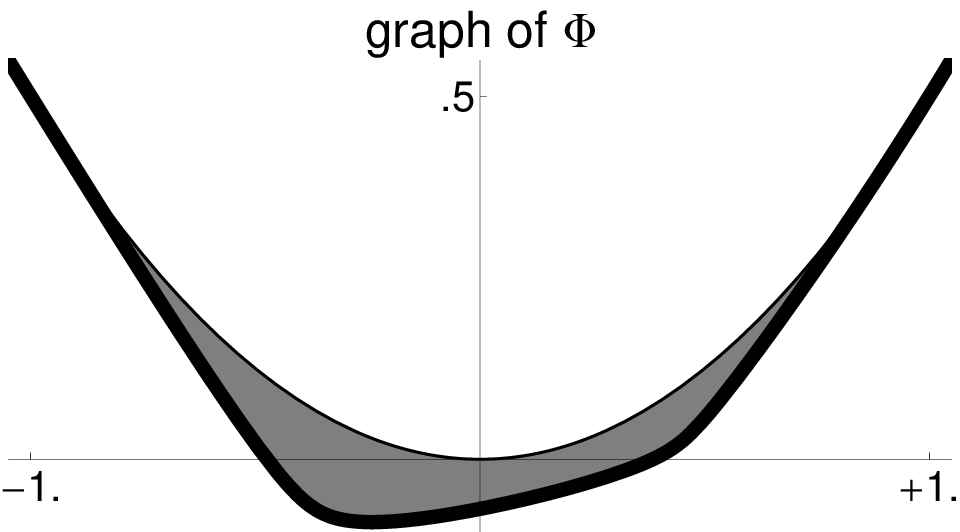
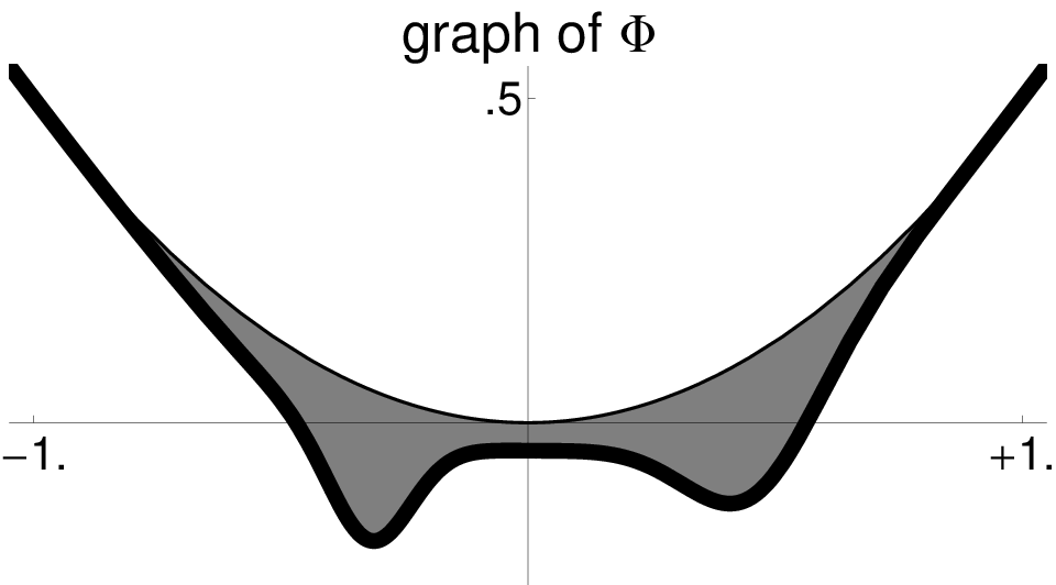
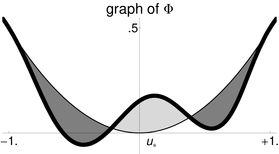
Figure 1: To each front there exists a parabola that touches the graph of Φ\Phi in both r−r_{-} and r+r_{+}. Consequently, the signed area between the graph of Φ′\Phi^{\prime} and the secant connecting r−r_{-} and r+r_{+} vanishes the stripe [r−,r+][r_{-},\,r_{+}].
Lemma 3.

The following conditions are equivalent:

  1. (i){\left({i}\right)}

    (σ,r−,r+){\left({{\sigma}},\,{r_{-}},\,{r_{+}}\right)} fulfils (10),

  2. (i​i){\left({ii}\right)}

    there exists a parabola that touches the graph of Φ\Phi in both r−r_{-} and r+r_{+},

  3. (i​i​i){\left({iii}\right)}

    the signed area between the graph of Φ′\Phi^{\prime} and the secant connecting r−r_{-} to r+r_{+} sums up to zero in [r−,r+][r_{-},\,r_{+}].

Moreover, each condition implies that Φ′\Phi^{\prime} has at least one turning point between r−r_{-} and r+r_{+}.

Proof.

Consider the parabola f⁡(r)=12​a​r2+b​r+cf{\left({r}\right)}=\tfrac{1}{2}ar^{2}+br+c. The touching conditions

f⁡(r±)=Φ⁡(r±),f′​(r±)=Φ′​(r±)\displaystyle f{\left({r_{\pm}}\right)}=\Phi{\left({r_{\pm}}\right)},\quad f^{\prime}{\left({r_{\pm}}\right)}=\Phi^{\prime}{\left({r_{\pm}}\right)}

are equivalent to

12​a​|[r2]|+b​|[r]|=|[Φ⁡(r)]|,12​a​⟨r2⟩+b⁡⟨r⟩+c=⟨Φ⁡(r)⟩,|[r]|​a=|[Φ′​(r)]|,a⁡⟨r⟩+b=⟨Φ′​(r)⟩,\displaystyle\tfrac{1}{2}a{|\![r^{2}]\!|}+b{|\![r]\!|}={|\![\Phi{\left({r}\right)}]\!|},\quad\tfrac{1}{2}a{\langle r^{2}\rangle}+b{\langle r\rangle}+c={\langle\Phi{\left({r}\right)}\rangle},\quad{|\![r]\!|}a={|\![\Phi^{\prime}{\left({r}\right)}]\!|},\quad a{\langle r\rangle}+b={\langle\Phi^{\prime}{\left({r}\right)}\rangle},

and by 12​|[r2]|=⟨r⟩​|[r]|\tfrac{1}{2}{|\![r^{2}]\!|}={\langle r\rangle}{|\![r]\!|} we conclude that (i){\left({i}\right)} and (i​i){\left({ii}\right)} are equivalent via

a=σ2,b=⟨Φ′​(r)⟩−σ2​⟨r⟩,c=\displaystyle a={\sigma}^{2},\quad b={\langle\Phi^{\prime}{\left({r}\right)}\rangle}-{\sigma}^{2}{\langle r\rangle},\quad{c}= ⟨Φ⁡(r)⟩−⟨r⟩​⟨Φ′​(r)⟩+σ2​(⟨r⟩2−12​⟨r2⟩).\displaystyle{\langle\Phi{\left({r}\right)}\rangle}-{\langle r\rangle}{\langle\Phi^{\prime}{\left({r}\right)}\rangle}+{\sigma}^{2}{\big({\langle r\rangle}^{2}-\tfrac{1}{2}{\langle r^{2}\rangle}\big)}.

The equivalence of (i​i){\left({ii}\right)} and (i​i​i){\left({iii}\right)} is immediate since the secant has slope σ2{\sigma}^{2}, and Φ′\Phi^{\prime} must have a turning point because otherwise the graph of Φ′\Phi^{\prime} would be either below or above the secant. ∎

Condition (10)1 is the kinetic relation for fronts and reveals that the asymptotic states cannot be chosen arbitrarily. More precisely, for given r−r_{-} and r+r_{+} we can choose σ{\sigma} and |[v]|{|\![v]\!|} such that the first two jump conditions in (7) (which correspond to mass and momentum) are satisfied. However, for the energy condition (7)3 to hold, r−r_{-} and r+r_{+} must additionally fulfil (10)1. Form this we conclude that fronts do not exist if Φ′\Phi^{\prime} is either convex or concave, and that in general we cannot prescribe both r−r_{-} and r+r_{+}.


We emphasize that (7) is in general not sufficient for the existence of fronts, i.e., there exist energy conserving shocks in the p-system that can not be realized by a front in FPU. In fact, it was proven in [Ioo00] that fronts bifurcate from convex-concave but not from concave-convex turning points of Φ′\Phi^{\prime}. This disproves the existence of subsonic fronts with small jump heights although there exist the corresponding energy conserving shocks.

In order to prove the existence of action minimizing fronts we shall additionally to (7) require that the graph of Φ\Phi is below the parabola defined by the asymptotic states, see Assumption 5. In particular, our existence result provides a front for Example AA from Figure 1 but does not cover Example BB, see Remark 12 and the examples in §4.

2.2 Normalization and reformulation

For our analysis in §3 it is convenient to normalize the asymptotic states and to reformulate the front equation (5) as an eigenvalue problem for a nonlinear integral operator.

Lemma 4.

Up to affine transformations we can assume that

σ=1,r±=±1,v±=∓1,Φ′​(±1)=±1,Φ⁡(±1)=12.\displaystyle{\sigma}=1,\quad r_{\pm}=\pm 1,\quad v_{\pm}=\mp 1,\quad\Phi^{\prime}{\left({\pm 1}\right)}=\pm 1,\quad\Phi{\left({\pm 1}\right)}=\tfrac{1}{2}. (11)

Moreover, with (11) the front equation is equivalent to

W=𝒜​Φ′​(𝒜​W),(𝒜​W)​(φ)=∫φ−12φ−12W⁡(φ~)​𝑑φ~,\displaystyle W=\mathcal{A}{\Phi}^{\prime}{\left({\mathcal{A}{W}}\right)},\qquad{\left({\mathcal{A}{W}}\right)}{\left({{\varphi}}\right)}=\int\limits_{{\varphi}-\tfrac{1}{2}}^{{\varphi}-\tfrac{1}{2}}W{\left({\tilde{\varphi}}\right)}\,\mathrm{d}\tilde{\varphi}, (12)

where WW is a normalized profile with limφ→±∞W⁡(φ)=±1\lim_{{\varphi}\to\pm\infty}W{\left({{\varphi}}\right)}=\pm 1.

Proof.

Let UU and WW be two normalized profiles such that

R⁡(φ)=⟨r⟩+12​|[r]|​U​(φ+1/2),V⁡(φ)=⟨v⟩+12​|[v]|​W​(φ).\displaystyle{R}{\left({{\varphi}}\right)}={\langle r\rangle}+\tfrac{1}{2}{|\![r]\!|}U{\left({{\varphi}+1/2}\right)},\qquad V{\left({{\varphi}}\right)}={\langle v\rangle}+\tfrac{1}{2}{|\![v]\!|}W{\left({{\varphi}}\right)}.

Using the first two jump conditions from (7) we readily verify that (5) transforms into

dd​φ​U​(φ)=W⁡(φ+1/2)−W⁡(φ−1/2),dd​φ​W​(φ)=Φ^′​(U⁡(φ+1/2))−Φ^′​(U⁡(φ−1/2)),\displaystyle\tfrac{\,\mathrm{d}}{\,\mathrm{d}{\varphi}}U{\left({{\varphi}}\right)}=W{\left({{\varphi}+1/2}\right)}-W{\left({{\varphi}-1/2}\right)},\qquad\tfrac{\,\mathrm{d}}{\,\mathrm{d}{\varphi}}W{\left({{\varphi}}\right)}={\widehat{\Phi}}^{\prime}{\big(U{\left({{\varphi}+1/2}\right)}\big)}-{\widehat{\Phi}}^{\prime}{\big(U{\left({{\varphi}-1/2}\right)}\big)}, (13)

where the normalized potential

Φ^​(u)=4|[Φ′​(r)]|​|[r]|​Φ​(⟨r⟩+12​|[r]|​u)−2​⟨Φ′​(r)⟩|[Φ′​(r)]|​u+12−4​⟨Φ⁡(r)⟩|[Φ′​(r)]|​|[r]|\displaystyle{\widehat{\Phi}}{\left({u}\right)}=\frac{4}{{|\![\Phi^{\prime}{\left({r}\right)}]\!|}{|\![r]\!|}}{\Phi}{\Big({\langle r\rangle}+\tfrac{1}{2}{|\![r]\!|}\,u\Big)}-\frac{2{\langle\Phi^{\prime}{\left({r}\right)}\rangle}}{{|\![\Phi^{\prime}{\left({r}\right)}]\!|}}\,{u}+\frac{1}{2}-\frac{4{\langle\Phi{\left({r}\right)}\rangle}}{{|\![\Phi^{\prime}{\left({r}\right)}]\!|}{|\![r]\!|}}

satisfies Φ^′​(±1)=±1{\widehat{\Phi}}^{\prime}{\left({\pm 1}\right)}=\pm 1. Moreover, we have Φ^​(−1)=Φ^​(+1)=12{\widehat{\Phi}}{\left({-1}\right)}={\widehat{\Phi}}{\left({+1}\right)}=\tfrac{1}{2} if and only if the third jump condition (7)3 is satisfied. Towards (12) now suppose (11). Integrating (13)1 we find U=𝒜​WU=\mathcal{A}{W}, where the constant of integration vanishes due to U⁡(±1)=W⁡(±1)=±1U{\left({\pm 1}\right)}=W{\left({\pm 1}\right)}=\pm 1, and similarly we derive W=𝒜​Φ^′​(U)W=\mathcal{A}{\widehat{\Phi}}^{\prime}{\left({U}\right)} from (13)2. ∎

The front parabola for normalized data (11) is r↦12​r2r\mapsto\tfrac{1}{2}r^{2} and each solution to (12) can be viewed as a perturbation of the shock profile

Wsh​(φ)=sgn​φ={+1forφ<0,0forφ=0,−1forφ>0.\displaystyle W_{\rm sh}{\left({{\varphi}}\right)}=\mathrm{sgn}{\varphi}=\left\{\begin{array}[]{rcl}+1&\text{for}&{\varphi}<0,\\ 0&\text{for}&{\varphi}=0,\\ -1&\text{for}&{\varphi}>0.\end{array}\right.

Notice that the residual of WshW_{\rm sh}, that is Wsh−𝒜​Φ′​(𝒜​Wsh)W_{\rm sh}-\mathcal{A}\Phi^{\prime}{\left({\mathcal{A}{W_{\rm sh}}}\right)}, has compact support.


We proceed with some preliminary remarks about the action of a front. Heuristically, the action density in the normalized setting is given by

12​W2−Φ⁡(𝒜​W)=12​W2−12​(𝒜​W)2+Ψ⁡(𝒜​W)\displaystyle\tfrac{1}{2}W^{2}-\Phi{\left({\mathcal{A}{W}}\right)}=\tfrac{1}{2}W^{2}-\tfrac{1}{2}{\left({\mathcal{A}{W}}\right)}^{2}+\Psi{\left({\mathcal{A}{W}}\right)}

with

Ψ⁡(r)=12​r2−Φ⁡(r),\displaystyle\Psi{\left({r}\right)}=\tfrac{1}{2}r^{2}-\Phi{\left({r}\right)}, (17)

so the action integral formally reads

ℒ~​(W)\displaystyle{\widetilde{\mathcal{L}}}{\left({W}\right)} =∫ℝ12​W2−12​(𝒜​W)2+Ψ⁡(𝒜​W)​𝑑φ.\displaystyle=\int\limits_{\mathbb{R}}\tfrac{1}{2}W^{2}-\tfrac{1}{2}{\left({\mathcal{A}{W}}\right)}^{2}+\Psi{\left({\mathcal{A}{W}}\right)}\,\mathrm{d}{\varphi}. (18)

Notice that Ψ\Psi is just the difference between the front parabola and Φ\Phi, see Figure 1, and that ℒ~{\widetilde{\mathcal{L}}} is well defined as long as WW approaches its asymptotic states sufficiently fast. A further possibility for defining the action integral was introduced in [HR09] for monotone WW and relies on the relative action integral

ℒ^​(W)\displaystyle{\widehat{\mathcal{L}}}{\left({W}\right)} =∫ℝ(12​W2−Φ⁡(𝒜​W))−(12​Wsh2−Φ⁡(𝒜​Wsh))​𝑑φ.\displaystyle=\int\limits_{\mathbb{R}}{\Big(\tfrac{1}{2}W^{2}-\Phi{\left({\mathcal{A}{W}}\right)}\Big)}-{\Big(\tfrac{1}{2}W_{\rm sh}^{2}-\Phi{\left({\mathcal{A}{W_{\rm sh}}}\right)}\Big)}\,\mathrm{d}{\varphi}.

Both approaches are linked by ℒ^​(W)=ℒ~​(W)−ℒ~​(Wsh){\widehat{\mathcal{L}}}{\left({W}\right)}={\widetilde{\mathcal{L}}}{\left({W}\right)}-{\widetilde{\mathcal{L}}}{\left({W_{\rm sh}}\right)} and the symmetry of 𝒜\mathcal{A}, compare Lemma 7, formally implies

∂ℒ^​(W)=∂ℒ~​(W)=W−𝒜​Φ′​(𝒜​W).\displaystyle\partial{\widehat{\mathcal{L}}}{\left({W}\right)}=\partial{\widetilde{\mathcal{L}}}{\left({W}\right)}=W-\mathcal{A}\Phi^{\prime}{\left({\mathcal{A}{W}}\right)}.

In §3 we give a slightly different definition of ℒ~{\widetilde{\mathcal{L}}}, see (20) and (25), and establish the existence of minimizers.

3 Existence of fronts

In this section we assume that the asymptotic states and the potential are normalized by (11) and show that the fixed point equation (12) has a solution in some appropriate function space.

3.1 Assumptions

We rely on the following standing assumptions on the function Ψ\Psi from (17). Examples and counterexamples are given in §4.

Assumption 5.

Ψ\Psi is continuously differentiable and satisfies the following conditions:

  1. (G)

    graph condition: Ψ⁡(u)≥Ψ⁡(±1)=0\Psi{\left({u}\right)}\geq\Psi{\left({\pm 1}\right)}=0 for all u∈ℝu\in{\mathbb{R}},

  2. (X)

    genericity: Ψ′′​(±1)>0\Psi^{\prime\prime}{\left({\pm 1}\right)}>0 and Ψ⁡(u)>0\Psi{\left({u}\right)}>0 for all u≠±1u\neq\pm 1,

  3. (M)

    monotone asymptotic behaviour: Ψ⁡(u)\Psi{\left({u}\right)} is decreasing for u≪−1u\ll-1 and increasing for u≫1u\gg 1.

Condition (G) has a natural interpretation in terms of Φ\Phi and can easily be reformulated for non-normalized data: It precisely means that the front parabola touches the graph of Φ\Phi in both r−r_{-} and r+r_{+} but is above this graph in all other points. Moreover, (G) is equivalent to the area condition from [HR09], which characterizes the signed area between the graph of Φ′\Phi^{\prime} and the secant connecting r−r_{-} to r+r_{+}. With positive and negative sign for above and below the graph of Φ′\Phi^{\prime}, respectively, the area condition reads as follows. The signed area is non-negative in each stripe [r−,r][r_{-},\,r] with r>r−r>r_{-} and non-positive in each stripe [r,r+][r,\,r_{+}] with r<r+r<r_{+}. We refer to Figure 1 for illustration, where positive and negative area are displayed in dark and light grey colour, respectively, and recall that the signed area vanishes in the stripe [r−,r+][r_{-},\,r_{+}] due to (10)1.

We mention that (G) is truly necessary for the existence of action minimizing fronts, see Remark 12. The conditions (M) and (X), however, are made for convenience and might be weakened for the price of more technical effort.

Remark 6.

(X) is equivalent to

  1. (S)

    supersonic front speed: Φ′′​(±1)<1\Phi^{\prime\prime}{\left({\pm 1}\right)}<1,

and (M) implies

  1. (I)

    invariant set for Φ′\Phi^{\prime}: There exits a constant Γ>1\Gamma>1 such that Φ′\Phi^{\prime} maps [−Γ,Γ][-\Gamma,\,\Gamma] into itself.

Proof.

(S) follows from the definition of Ψ\Psi in (17). Towards (I) we exploit (M) to choose Γ~>1\tilde{\Gamma}>1 such that Φ′​(u)>u\Phi^{\prime}{\left({u}\right)}>u for u<−Γ~u<-\tilde{\Gamma} and Φ′​(u)<u\Phi^{\prime}{\left({u}\right)}<u for u>Γ~u>\tilde{\Gamma}. Then we set Γ=max⁡{Γ~,max|u|≤Γ~⁡|Φ′​(u)|}\Gamma=\max\{\tilde{\Gamma},\,\max_{\left|{u}\right|\leq{\tilde{\Gamma}}}\left|{\Phi^{\prime}{\left({u}\right)}}\right|\}. ∎

3.2 Functionals and operators

We denote by 𝖫p{\mathsf{L}}^{p}, 𝖶1,p{\mathsf{W}}^{1,\,p} and 𝖢k{\mathsf{C}}^{k} the usual function spaces on the real line, abbreviate the 𝖫p{\mathsf{L}}^{p}-norm by ∥⋅∥p\|{\cdot}\|_{p}, and write

⟨W1,W2⟩=∫ℝW1​(φ)​W2​(φ)​𝑑φ\displaystyle{\left\langle{W_{1}},\,{W_{2}}\right\rangle}=\int_{\mathbb{R}}{W_{1}{\left({{\varphi}}\right)}}{W_{2}}{\left({{\varphi}}\right)}\,\mathrm{d}{\varphi}

for the dual pairing of W1∈𝖫pW_{1}\in{\mathsf{L}}^{p} and W2∈𝖫p′W_{2}\in{\mathsf{L}}^{p^{\prime}} with 1=1/p+1/p′1=1/p+1/p^{\prime}.

Lemma 7.

The averaging operator 𝒜\mathcal{A} has the following properties:

  1. 1.

    𝒜\mathcal{A} maps 𝖫p{\mathsf{L}}^{p} into 𝖫∞∩𝖶1,p⊂𝖢{\mathsf{L}}^{\infty}\cap{\mathsf{W}}^{1,\,p}\subset{\mathsf{C}} for all 1≤p≤∞1\leq{p}\leq\infty with

    (𝒜​W)′​(φ)=W⁡(φ+12)−W⁡(φ−12)\displaystyle{\left({\mathcal{A}{W}}\right)}^{\prime}{\left({{\varphi}}\right)}=W{\left({{\varphi}+\tfrac{1}{2}}\right)}-W{\left({{\varphi}-\tfrac{1}{2}}\right)}

    and ‖𝒜​W‖𝖫p≤‖W‖𝖫p\|{\mathcal{A}{W}}\|_{{\mathsf{L}}^{p}}\leq\|{W}\|_{{\mathsf{L}}^{p}}, ‖𝒜​W‖𝖫∞≤‖W‖𝖫p\|{\mathcal{A}{W}}\|_{{\mathsf{L}}^{\infty}}\leq\|{W}\|_{{\mathsf{L}}^{p}}, ‖𝒜​W‖𝖶1,p≤3​‖W‖𝖫p\|{\mathcal{A}{W}}\|_{{\mathsf{W}}^{1,\,p}}\leq 3\|{W}\|_{{\mathsf{L}}^{p}}.

  2. 2.

    𝒜\mathcal{A} is symmetric in the sense that ⟨𝒜​W1,W2⟩=⟨W1,𝒜​W2⟩{\left\langle{\mathcal{A}{W_{1}}},\,{W_{2}}\right\rangle}={\left\langle{W_{1}},\,{\mathcal{A}{W_{2}}}\right\rangle} holds for all W1∈𝖫pW_{1}\in{\mathsf{L}}^{p} and W2∈𝖫p′W_{2}\in{\mathsf{L}}^{p^{\prime}}.

  3. 3.

    𝒜\mathcal{A} is self-adjoint in 𝖫2{\mathsf{L}}^{2} with spectrum spec​𝒜={ϱ⁡(k):k∈ℝ}\mathrm{spec}\mathcal{A}=\{\varrho{\left({k}\right)}\;:\;k\in{\mathbb{R}}\} where ϱ⁡(k)=2k​sin⁡(k2)\varrho{\left({k}\right)}=\tfrac{2}{k}\sin{\left({\tfrac{k}{2}}\right)}.

Proof.

The first two statements are straight forward. The third one follows since 𝒜\mathcal{A} diagonalizes in Fourier space via 𝒜​𝚎𝚒​k​φ=ϱ⁡(k)​𝚎𝚒​k​φ\mathcal{A}{{\mathtt{e}}^{\mathtt{i}{k}{\varphi}}}=\varrho{\left({k}\right)}{{\mathtt{e}}^{\mathtt{i}{k}{\varphi}}}. ∎

We now introduce the affine space

ℋ={W:W−Wsh∈𝖫2},\displaystyle\mathcal{H}=\left\{W\;:\;W-W_{\rm sh}\in{\mathsf{L}}^{2}\right\},

where WshW_{\rm sh} is the shock profile from (2.2). Exploiting Lemma 7, the Taylor expansion of Φ′\Phi^{\prime} around ±1\pm 1, and the properties of WshW_{\rm sh} we then find

𝒜​W,Φ′​(𝒜​W),𝒜​Φ′​(𝒜​W)∈ℋ,W−𝒜​W,W−𝒜2​W∈𝖫2.\displaystyle\mathcal{A}{W},\;\Phi^{\prime}{\left({\mathcal{A}{W}}\right)},\;\mathcal{A}\Phi^{\prime}{\left({\mathcal{A}{W}}\right)}\in\mathcal{H},\qquad W-\mathcal{A}{W},\;W-\mathcal{A}^{2}{W}\in{\mathsf{L}}^{2}. (19)

for all W∈ℋW\in\mathcal{H}. In view of the action integral (18) we also define a functional ℳ\mathcal{M} on 𝖫2{\mathsf{L}}^{2} by

ℳ⁡(V)=12​∫ℝV2−(𝒜​V)2​𝑑φ=12​∫ℝ(V−𝒜2​V)​V​𝑑φ,\displaystyle\mathcal{M}(V)=\tfrac{1}{2}\int\limits_{\mathbb{R}}V^{2}-(\mathcal{A}{V})^{2}\,\mathrm{d}{\varphi}=\tfrac{1}{2}\int\limits_{\mathbb{R}}(V-\mathcal{A}^{2}V)V\,\mathrm{d}{\varphi},

and a functional 𝒩\mathcal{N} on ℋ\mathcal{H} by

𝒩⁡(W)=ℳ⁡(W−Wsh)+12​∫ℝWsh2−(𝒜​Wsh)2​𝑑φ+∫ℝ(W−Wsh)​(Wsh−𝒜2​Wsh)​𝑑φ.\displaystyle\mathcal{N}{\left({W}\right)}=\mathcal{M}{\left({W-W_{\rm sh}}\right)}+\tfrac{1}{2}\int\limits_{\mathbb{R}}W_{\rm sh}^{2}-{\left({\mathcal{A}{W_{\rm sh}}}\right)}^{2}\,\mathrm{d}{\varphi}+\int\limits_{\mathbb{R}}{\left({W-W_{\rm sh}}\right)}{\left({W_{\rm sh}-\mathcal{A}^{2}{W_{\rm sh}}}\right)}\,\mathrm{d}{\varphi}. (20)

Notice that 𝒩⁡(W)\mathcal{N}{\left({W}\right)} is well defined on ℋ\mathcal{H} as both Wsh2−(𝒜​Wsh)2W_{\rm sh}^{2}-{\left({\mathcal{A}{W_{\rm sh}}}\right)}^{2} and Wsh−𝒜2​WshW_{\rm sh}-\mathcal{A}^{2}{W_{\rm sh}} have compact support. Moreover, if W−WshW-W_{\rm sh} decays sufficiently fast for φ→±∞{\varphi}\to\pm\infty (say W−Wsh∈𝖫1W-W_{\rm sh}\in{\mathsf{L}}^{1}), then we have

𝒩⁡(W)=12​∫ℝW2−(𝒜​W)2​𝑑φ=12​∫ℝ(W−𝒜2​W)​W​𝑑φ.\displaystyle\mathcal{N}{\left({W}\right)}=\tfrac{1}{2}\int\limits_{\mathbb{R}}W^{2}-{\left({\mathcal{A}{W}}\right)}^{2}\,\mathrm{d}{\varphi}=\tfrac{1}{2}\int\limits_{\mathbb{R}}{\left({W-\mathcal{A}^{2}W}\right)}W\,\mathrm{d}{\varphi}. (21)
Lemma 8.

The functional ℳ\mathcal{M} is non-negative and weakly lower semi-continuous on 𝖫2{\mathsf{L}}^{2}.

Proof.

Denoting the Fourier transform of VV by V^{\widehat{V}} we find

ℳ⁡(V)\displaystyle\mathcal{M}{\left({V}\right)} =∫ℝ(1−ϱ​(k)2)​V^​(k)2​𝑑k=‖1−ϱ2​V^‖2\displaystyle=\int\limits_{\mathbb{R}}(1-\varrho{\left({k}\right)}^{2}){\widehat{V}}{\left({k}\right)}^{2}\,\mathrm{d}k=\|{\sqrt{1-\varrho^{2}}\,{\widehat{V}}}\|_{2}

with ϱ\varrho as in Lemma 7. This gives the desired result as Vn⇀V∞V_{n}\rightharpoonup{V_{\infty}} implies V^n⇀V^∞{\widehat{V}}_{n}\rightharpoonup{{\widehat{V}}_{\infty}} and hence 1−ϱ2​V^n⇀1−ϱ2​V^∞\sqrt{1-\varrho^{2}}\,{\widehat{V}}_{n}\rightharpoonup{\sqrt{1-\varrho^{2}}\,{\widehat{V}}_{\infty}} ∎

Lemma 9.

The functional 𝒩\mathcal{N} is Gâteaux differentiable on ℋ\mathcal{H} with derivative

∂𝒩⁡(W)=W−𝒜2​W∈𝖫2.\displaystyle\partial\mathcal{N}{\left({W}\right)}=W-\mathcal{A}^{2}{W}\in{\mathsf{L}}^{2}. (22)

Moreover, 𝒩\mathcal{N} is invariant under shifts in φ{\varphi}-direction, and satisfies

𝒩⁡(W2)=𝒩⁡(W1)+ℳ⁡(W2−W1)+⟨W2−W1,W1−𝒜2​W1⟩\displaystyle\mathcal{N}{\left({W_{2}}\right)}=\mathcal{N}{\left({W_{1}}\right)}+\mathcal{M}{\left({W_{2}-W_{1}}\right)}+{\left\langle{W_{2}-W_{1}},\,{W_{1}-\mathcal{A}^{2}{W}_{1}}\right\rangle} (23)

for all W1,W2∈ℋW_{1},\,W_{2}\in\mathcal{H}.

Proof.

A direct computation with W∈ℋW\in\mathcal{H} and δ​W∈𝖫2\delta{W}\in{\mathsf{L}}^{2} shows

⟨∂𝒩⁡(W),δ​W⟩\displaystyle{\left\langle{\partial\mathcal{N}{\left({W}\right)}},\,{\delta{W}}\right\rangle} =(⟨W−Wsh,δ​W⟩−⟨𝒜​W−𝒜​Wsh,𝒜​δ​W⟩)+⟨Wsh−𝒜2​Wsh,δ​W⟩\displaystyle={\big({\left\langle{W-W_{\rm sh}},\,{\delta{W}}\right\rangle}-{\left\langle{\mathcal{A}{W}-\mathcal{A}{W_{\rm sh}}},\,{\mathcal{A}{\delta{W}}}\right\rangle}\big)}+{\left\langle{W_{\rm sh}-\mathcal{A}^{2}{W_{\rm sh}}},\,{\delta{W}}\right\rangle}
=⟨W−Wsh,δ​W⟩−⟨𝒜2​W−𝒜2​Wsh,δ​W⟩+⟨Wsh−𝒜2​Wsh,δ​W⟩\displaystyle={\left\langle{W-W_{\rm sh}},\,{\delta{W}}\right\rangle}-{\left\langle{\mathcal{A}^{2}{W}-\mathcal{A}^{2}{W_{\rm sh}}},\,{\delta{W}}\right\rangle}+{\left\langle{W_{\rm sh}-\mathcal{A}^{2}{W_{\rm sh}}},\,{\delta{W}}\right\rangle}
=⟨W−𝒜2,δ​W⟩,\displaystyle={\left\langle{W-\mathcal{A}^{2}},\,{\delta{W}}\right\rangle},

and this gives (22). Towards the shift invariance we approximate WW by

Wn=χ[−n,n]​(W−Wsh)+Wsh\displaystyle W_{n}=\chi_{[-n,\,n]}{\left({W-W_{\rm sh}}\right)}+W_{\rm sh}

where χ[−n,n]\chi_{[-n,\,n]} is the indicator function of the interval [−n,n][-n,\,n]. Then we use (21) for WnW_{n} to find ℒ(Wn)=ℒ(Wn(⋅+φ¯))\mathcal{L}{\left({W_{n}}\right)}=\mathcal{L}{\left({W_{n}{\left({\cdot+\bar{\varphi}}\right)}}\right)} for all shifts φ¯\bar{\varphi}, and passing to the limit n→∞n\to\infty gives the desired result. Finally, by definition we have

𝒩⁡(W2)−𝒩⁡(W1)\displaystyle\mathcal{N}{\left({W_{2}}\right)}-\mathcal{N}{\left({W_{1}}\right)} =ℳ⁡(W2−Wsh)−ℳ⁡(W1−Wsh)+⟨W2−W1,Wsh−𝒜2​Wsh⟩\displaystyle=\mathcal{M}{\left({W_{2}-W_{\rm sh}}\right)}-\mathcal{M}{\left({W_{1}-W_{\rm sh}}\right)}+{\left\langle{W_{2}-W_{1}},\,{W_{\rm sh}-\mathcal{A}^{2}W_{\rm sh}}\right\rangle}

and

ℳ⁡(W2−Wsh)−ℳ⁡(W1−Wsh)=ℳ⁡(W2−W1)+⟨W2−W1,W1−Wsh−𝒜2​W1+𝒜2​Wsh⟩,\displaystyle\mathcal{M}{\left({W_{2}-W_{\rm sh}}\right)}-\mathcal{M}{\left({W_{1}-W_{\rm sh}}\right)}=\mathcal{M}{\left({W_{2}-W_{1}}\right)}+{\left\langle{W_{2}-W_{1}},\,{W_{1}-W_{\rm sh}-\mathcal{A}^{2}{W_{1}}+\mathcal{A}^{2}{W_{\rm sh}}}\right\rangle},

so (23) follows from adding both identities. ∎

To conclude this section we consider the functional

𝒫⁡(W)=∫ℝΨ⁡(𝒜​W)​𝑑φ,\displaystyle\mathcal{P}{\left({W}\right)}=\int\limits_{\mathbb{R}}{}\Psi{\left({\mathcal{A}{W}}\right)}\,\mathrm{d}{\varphi},

which gives the non-quadratic part of the action integral (18)

Lemma 10.

𝒫\mathcal{P} is well defined on ℋ\mathcal{H} with

c¯​‖𝒜​W−sgn⁡(𝒜​W)‖2≤𝒫⁡(W)≤c¯​‖𝒜​W−sgn⁡(𝒜​W)‖2\displaystyle\underline{c}\|{\mathcal{A}{W}-\mathrm{sgn}{\left({\mathcal{A}{W}}\right)}}\|_{2}\leq\mathcal{P}{\left({W}\right)}\leq{\overline{c}}\|{\mathcal{A}{W}-\mathrm{sgn}{\left({\mathcal{A}{W}}\right)}}\|_{2} (24)

for some constants c¯\underline{c} and c¯{\overline{c}} that depend only on ‖A​W‖∞\|{AW}\|_{\infty}. Moreover, 𝒫\mathcal{P} is Gâteaux differentiable on ℋ\mathcal{H} with derivative ∂𝒫⁡(W)=𝒜2​W−𝒜​Φ′​(𝒜​W)\partial\mathcal{P}{\left({W}\right)}=\mathcal{A}^{2}{W}-\mathcal{A}\Phi^{\prime}{\left({\mathcal{A}{W}}\right)}.

Proof.

Let W∈ℋW\in\mathcal{H} be given and recall that U=𝒜​WU=\mathcal{A}{W} satisfies U∈ℋ∩𝖫∞U\in\mathcal{H}\cap{\mathsf{L}}^{\infty} due to Lemma 7. Condition (X) provides two constants c¯\underline{c} and c¯{\overline{c}} such that

c¯​(u−sgn​u)2≤Ψ⁡(u)≤c¯​(u−sgn​u)2\displaystyle\underline{c}{\left({u-\mathrm{sgn}{u}}\right)}^{2}\leq\Psi{\left({u}\right)}\leq{\overline{c}}{\left({u-\mathrm{sgn}{u}}\right)}^{2}\quad\text{}\quad

holds for all |u|≤‖U‖∞\left|{u}\right|\leq{\|{U}\|_{\infty}}, and we conclude that 𝒫\mathcal{P} is well defined and satisfies (24). Finally, (19) provides 𝒜2​W−𝒜​Φ′​(𝒜​W)∈𝖫2\mathcal{A}^{2}{W}-\mathcal{A}\Phi^{\prime}{\left({\mathcal{A}{W}}\right)}\in{\mathsf{L}}^{2}, so both the existence of and the formula for ∂𝒫\partial\mathcal{P} follow from a direct calculation. ∎

3.3 Variational setting

We now introduce the action functional on ℋ\mathcal{H} by

ℒ⁡(W)=𝒩⁡(W)+𝒫⁡(W).\displaystyle\mathcal{L}{\left({W}\right)}=\mathcal{N}{\left({W}\right)}+\mathcal{P}{\left({W}\right)}. (25)

In virtue of Lemma 9 and Lemma 10 the functional ℒ\mathcal{L} is well defined, shift invariant, and Gâteaux differentiable with derivative

∂ℒ⁡(W)=𝒜2​W−𝒜​Φ′​(𝒜​W)∈𝖫2,\displaystyle\partial\mathcal{L}{\left({W}\right)}=\mathcal{A}^{2}W-\mathcal{A}\Phi^{\prime}{\left({\mathcal{A}{W}}\right)}\in{\mathsf{L}}^{2},

and we conclude that each minimizer of ℒ\mathcal{L} in ℋ\mathcal{H} must solve the front equation (12). However, proving the existence of minimizers in ℋ\mathcal{H} turns out to be difficult and therefore we restrict ℒ\mathcal{L} to the convex subset

𝒞={W∈ℋ∩𝖶1,∞:∥W∥∞≤Γ,∥W′∥∞≤2Γ}.\displaystyle\mathcal{C}=\left\{W\in\mathcal{H}\cap{\mathsf{W}}^{1,\infty}\;:\;\|{W}\|_{\infty}\leq{{\Gamma}},\quad\|{W^{\prime}}\|_{\infty}\leq 2{{\Gamma}}\right\}.

Notice that the ansatz W∈𝒞W\in\mathcal{C} is reasonable due to condition (I)(I) and since the front equation (12) combined with Lemma 7 implies W∈ℋ∩𝖶1,∞W\in\mathcal{H}\cap{\mathsf{W}}^{1,\,\infty}.


In order to link fronts to minimizers of ℒ\mathcal{L} in 𝒞\mathcal{C} we observe that the properties of Φ′\Phi^{\prime} and 𝒜\mathcal{A} guarantee 𝒞\mathcal{C} to be invariant under the 𝖫2{\mathsf{L}}^{2}-gradient flow of ℒ\mathcal{L}. To see this we consider the explicit Euler scheme

W↦𝒯λ​(W)=W−λ​∂ℒ⁡(W)=(1−λ)​W+λ​𝒜​Φ′​(𝒜​W)\displaystyle W\mapsto\mathcal{T}_{\lambda}{\left({W}\right)}=W-{\lambda}\partial\mathcal{L}{\left({W}\right)}={\left({1-{\lambda}}\right)}W+{\lambda}\mathcal{A}\Phi^{\prime}{\left({\mathcal{A}{W}}\right)} (26)

with small step size λ{\lambda}.

Lemma 11.

The set 𝒞\mathcal{C} is invariant under the action of 𝒯λ\mathcal{T}_{\lambda} for 0<λ<10<{\lambda}<1. Consequently, each minimizer of ℒ\mathcal{L} in 𝒞\mathcal{C} solves the front equation (12).

Proof.

For W∈𝒞W\in\mathcal{C} let P=Φ′​(𝒜​W)P=\Phi^{\prime}{\left({\mathcal{A}{W}}\right)} and recall that 𝒜​W,P,𝒜​P∈ℋ\mathcal{A}{W},\;P,\;\mathcal{A}{P}\in\mathcal{H} according to (19). Combining (I) with ‖𝒜​W‖∞≤Γ\|{\mathcal{A}{W}}\|_{\infty}\leq{\Gamma} and (𝒜P)′=P(⋅+1/2)+P(⋅+1/2){\left({\mathcal{A}{P}}\right)}^{\prime}=P{\left({\cdot+1/2}\right)}+P{\left({\cdot+1/2}\right)} gives

‖P‖∞,‖𝒜​P‖∞≤Γ,‖(𝒜​P)′‖∞≤2​Γ,\displaystyle\|{P}\|_{\infty},\;\|{\mathcal{A}{P}}\|_{\infty}\leq{{\Gamma}},\qquad\|{{\left({\mathcal{A}{P}}\right)}^{\prime}}\|_{\infty}\leq 2{{\Gamma}},

and hence 𝒜​P∈𝒞\mathcal{A}{P}\in\mathcal{C}. Since 𝒞\mathcal{C} is convex we also have 𝒯λ​(W)∈𝒞\mathcal{T}_{\lambda}{\left({W}\right)}\in\mathcal{C} for all 0<λ<10<{\lambda}<1, and passing to the limit λ→0{\lambda}\to 0 we then establish the invariance of 𝒞\mathcal{C} under the 𝖫2{\mathsf{L}}^{2}-gradient flow of ℒ\mathcal{L}. In particular, each minimizer of ℒ\mathcal{L} in 𝒞\mathcal{C} must be a stationary point for the gradient flow of ℒ\mathcal{L} and hence a solution to the front equation. ∎

To complete the existence proof for fronts it remains to show that ℒ\mathcal{L} attains its minimum in 𝒞\mathcal{C}. We prove this in the next section by using the direct approach, that means we construct minimizers as limits of minimizing sequences.

A particular problem we have to overcome in the subsequent analysis is that ℒ\mathcal{L} is not coercive on ℋ\mathcal{H}. In fact, as illustrated in Figure 2 there exist sequences (Wn)n⊂𝒞{\left({W_{n}}\right)}_{n}\subset\mathcal{C} with extending plateaus at −1-1 or +1+1. These plateaus contribute neither to 𝒩\mathcal{N} nor 𝒫\mathcal{P} but may imply

∥Wn−Wsh(φn+⋅)∥2→n→∞∞\displaystyle\|{W_{n}-W_{\rm sh}{\left({{\varphi}_{n}+\cdot}\right)}}\|_{2}\xrightarrow{n\to\infty}\infty

for all choices of the relative shifts φn{\varphi}_{n}. Heuristically it is clear that the cartoon from Figure 2 cannot be prototypical for action minimizing sequences, but in order to proof this we need a better understanding of sequences with bounded action.

Figure 2: Sketch of a sequence with bounded action and two extending plateaus at ±1\pm 1: graphs of WnW_{n} and Un=𝒜​WnU_{n}=\mathcal{A}{W_{n}} in Black in Gray, respectively. The shaded areas indicate corresponding separations of phases with In,j=φn,j+JjI_{n,j}={\varphi}_{n,j}+J_{j} as in Lemma 15.

We conclude with a remark about the necessity of the graph condition (G) and refer to §4 for numerical examples.

Remark 12.

Suppose that Ψ\Psi satisfies (M)(M), (X)(X), and Ψ⁡(±1)=0\Psi{\left({\pm 1}\right)}=0, but violates (G) because there is some u∗u_{\ast} with |u∗|<Γ\left|{u_{\ast}}\right|<{\Gamma} and Ψ⁡(u∗)<0\Psi{\left({u_{\ast}}\right)}<0. Then ℒ\mathcal{L} is unbounded from below.

Proof.

We define a sequence (Wn)n⊂ℋ{\left({W_{n}}\right)}_{n}\subset\mathcal{H} of piecewise linear profiles by Wn​(φ)=u∗W_{n}{\left({{\varphi}}\right)}=u_{\ast} for |φ|≤n\left|{{\varphi}}\right|\leq{n} and Wn​(φ)=sgn​φW_{n}{\left({{\varphi}}\right)}=\mathrm{sgn}{\varphi} for |φ|≥n+1/Γ\left|{{\varphi}}\right|\geq{n+1/{\Gamma}}. By construction, Wn−𝒜2​WnW_{n}-\mathcal{A}^{2}{W}_{n} is supported in In∪(−In)I_{n}\cup{\left({-I_{n}}\right)} with In=[n−1,n+1+Γ]I_{n}=[n-1,\,n+1+{\Gamma}], and a direct calculation shows

ℒ⁡(Wn)≤C+2​(n−1)​Ψ​(u∗)→n→∞−∞,\displaystyle\mathcal{L}{\left({W_{n}}\right)}\leq{C}+2{\left({n-1}\right)}\Psi{\left({u_{\ast}}\right)}\xrightarrow{n\to\infty}-\infty,

where CC is some constant independent of nn. ∎

3.4 Separation of phases for sequences with bounded 𝒫\mathcal{P}

To characterize the qualitative properties of a profile U=𝒜​WU=\mathcal{A}{W} with W∈𝒞W\in\mathcal{C} we interpret U<12U<\tfrac{1}{2} and U>12U>\tfrac{1}{2} as negative phase and positive phase, respectively, and regard intervals in which UU takes intermediate values as transition layers. Obviously, adjacent plateaus of different height are separated by a transition layer and each UU must exhibit at least one transition layer as it connects −1-1 to +1+1.

We next exploit the uniform 𝖫∞{\mathsf{L}}^{\infty}-bound for W∈𝒞W\in\mathcal{C} to derive a lower bound for the 𝒫\mathcal{P}-contribution of each transition layer. To this end we introduce

ZU={φ¯:|U⁡(φ¯)|≤12}.\displaystyle Z_{U}=\{\bar{\varphi}\;:\;\left|{U{\left({\bar{\varphi}}\right)}}\right|\leq\tfrac{1}{2}\}.

which is nonempty, closed and bounded as U∈𝒞U\in\mathcal{C} is continuous with U⁡(φ)→±1U{\left({{\varphi}}\right)}\to\pm 1 as φ→±∞{\varphi}\to\pm\infty.

Remark 13.

There exist constants η¯>0\bar{\eta}>0 and μ¯>0\bar{\mu}>0 such that

∫φ¯−η¯φ¯+η¯Ψ⁡(U⁡(φ))​𝑑φ>μ¯\displaystyle\int\limits_{\bar{\varphi}-\bar{\eta}}^{\bar{\varphi}+\bar{\eta}}\Psi{\left({U{\left({{\varphi}}\right)}}\right)}\,\mathrm{d}{\varphi}>\bar{\mu}

for each U∈𝒞U\in\mathcal{C} and φ¯∈ZU\bar{{\varphi}}\in{Z}_{U}.

Proof.

This follows since U∈𝒞U\in\mathcal{C} implies |U⁡(φ2)−U⁡(φ1)|≤∫φ2φ1|U′​(φ)|​𝑑φ≤2​Γ​|φ2−φ1|\left|{U{\left({{\varphi}_{2}}\right)}-U{\left({{\varphi}_{1}}\right)}}\right|\leq\int_{{\varphi}_{2}}^{{\varphi}_{1}}\left|{U^{\prime}{\left({{\varphi}}\right)}}\right|\,\mathrm{d}{\varphi}\leq 2\Gamma\left|{{\varphi}_{2}-{\varphi}_{1}}\right|. In particular, we have |U⁡(φ)|≤3/4\left|{U{\left({{\varphi}}\right)}}\right|\leq 3/4 for all |φ−φ¯|≤η¯=1/(8​Γ)\left|{{\varphi}-\bar{\varphi}}\right|\leq\bar{\eta}=1/{\left({8{\Gamma}}\right)} and the claim follows with μ¯=σ¯/(2​η¯)\bar{\mu}=\bar{\sigma}/{\left({2\bar{\eta}}\right)} and σ¯=sup|u|≤3/4Ψ⁡(u)>0\bar{\sigma}=\sup_{\left|{u}\right|\leq 3/4}\Psi{\left({u}\right)}>0. ∎

In order to show that each function UU possesses a finite number of transition layers we introduce the following definition. A separation of phases for a given profile U∈𝒞U\in\mathcal{C} is a finite collection of closed intervals (transition layers) I1,…,ImI_{1},\,{...},\,I_{m}, m≥1m\geq 1, such that

  1. 1.

    the intervals are disjoint and ordered, i.e.,

    min⁡I1<max⁡I1<min⁡I2<…<max⁡Im−1<min⁡Im<max⁡Im,\displaystyle\min{I_{1}}<\max{I_{1}}<\min{I_{2}}<{...}<\max{I_{m-1}}<\min{I_{m}}<\max{I_{m}},
  2. 2.

    ZUZ_{U} is contained in I1∪…∪ImI_{1}\cup{...}\cup{I_{m}}.

  3. 3.

    for each interval IjI_{j} there exists φ¯j∈ZU\bar{\varphi}_{j}\in{Z_{U}} such that with [φ¯j−η¯,φ¯j+η¯]⊂Ij[\bar{\varphi}_{j}-\bar{\eta},\,\bar{\varphi}_{j}+\bar{\eta}]\subset{I_{j}},

Lemma 14.

Let W∈𝒞W\in\mathcal{C} be given and set U=𝒜​WU=\mathcal{A}{W}. Then there exists a separation of phases I1,…,ImI_{1},\,{...},\,I_{m} for UU with

m≤floor⁡(𝒫⁡(W)/μ¯)and2​η¯≤|Ij|≤4​𝒫​(W)​η¯/μ¯\displaystyle m\leq\mathrm{floor}{\left({\mathcal{P}{\left({W}\right)}/\bar{\mu}}\right)}\quad\text{and}\quad 2\bar{\eta}\leq\left|{I_{j}}\right|\leq 4\mathcal{P}{\left({W}\right)}\bar{\eta}/\bar{\mu}

for all j=1​…​mj=1{...}{m}.

Proof.

We define a finite number of points φ¯j∈ZU\bar{{\varphi}}_{j}\in{Z_{U}} and intervals Ij=(φ¯j−2​η¯,φ¯j−2​η¯)I_{j}=(\bar{{\varphi}}_{j}-2\bar{\eta},\,\bar{{\varphi}}_{j}-2\bar{\eta}) iteratively as follows: φ¯1\bar{{\varphi}}_{1} is the smallest element of ZUZ_{U}, i.e. U⁡(φ)<−12U{\left({{\varphi}}\right)}<-\tfrac{1}{2} for all φ<φ¯1{\varphi}<\bar{{\varphi}}_{1}. If ZU∖I1Z_{U}\setminus{I_{1}} is empty we stop the iteration; otherwise we choose φ¯2\bar{{\varphi}}_{2} to be the smallest zero of ZUZ_{U} outside of I1I_{1}. Then we have φ¯2−φ¯1≥2​η¯\bar{{\varphi}}_{2}-\bar{{\varphi}}_{1}\geq 2\bar{\eta}, so Remark 13 yields

𝒫⁡(W)≥∫φ¯1−η¯φ¯1+η¯Ψ⁡(U⁡(φ))​𝑑φ+∫φ¯2−η¯φ¯2+η¯Ψ⁡(U⁡(φ))​𝑑φ≥2​μ¯.\displaystyle\mathcal{P}{\left({W}\right)}\geq\int\limits_{\bar{{\varphi}}_{1}-\bar{\eta}}^{\bar{{\varphi}}_{1}+\bar{\eta}}\Psi{\left({U{\left({{\varphi}}\right)}}\right)}\,\mathrm{d}{\varphi}+\int\limits_{\bar{{\varphi}}_{2}-\bar{\eta}}^{\bar{{\varphi}}_{2}+\bar{\eta}}\Psi{\left({U{\left({{\varphi}}\right)}}\right)}\,\mathrm{d}{\varphi}\geq{2}\bar{\mu}.

If possible, we now define φ¯3\bar{{\varphi}}_{3} as the minimum of ZU∖(I1∪I2)Z_{U}\setminus{\left({I_{1}\cup{I_{2}}}\right)} and proceed iteratively until the iteration stops after m≤floor⁡(𝒫⁡(W)/μ¯)m\leq\mathrm{floor}{\left({\mathcal{P}{\left({W}\right)}/\bar{\mu}}\right)} steps. By construction, we have ZU⊂⋃j=1mIjZ_{U}\subset\bigcup_{j=1}^{m}{I_{j}} and |Ij|≤4​η¯\left|{I_{j}}\right|\leq 4\bar{\eta} for all jj but the intervals IjI_{j} may overlap. Finally, we obtain the desired separation of phases by merging overlapping intervals. ∎

Our main result in this section concerns sequences (Wn)n∈𝒞{\left({W_{n}}\right)}_{n}\in\mathcal{C} with bounded 𝒫⁡(Wn)\mathcal{P}{\left({W_{n}}\right)}. It guarantees, roughly speaking, the existence of compatible transitions layers which (i){\left({i}\right)} have the same length, (i​i){\left({ii}\right)} separate the same phases, and (i​i​i){\left({iii}\right)} depart from each other. For an illustration we refer to Figure 2.

Lemma 15.

Let (Wn)n⊂𝒞{\left({W_{n}}\right)}_{n}\subset\mathcal{C} be a sequence with lim supn→∞𝒫⁡(Wn)<∞\limsup_{n\to\infty}\mathcal{P}{\left({W_{n}}\right)}<\infty. Then there exists a not relabelled subsequence along with a finite number of intervals J1,…,JmJ_{1},\,{...},\,J_{m} with the following properties:

  1. 1.

    Each interval JjJ_{j} is centred around zero, i.e., Jj=[−ηj,ηj]J_{j}=[-\eta_{j},\,\eta_{j}] for some 0<ηj<∞0<\eta_{j}<\infty.

  2. 2.

    For each nn there exist shifts φn,1<…<φn,m{\varphi}_{n,1}<{...}<{\varphi}_{n,m} such that

    1. (a)

      φn,1+J1,…,φn,m+Jm{\varphi}_{n,1}+J_{1},\,{...},\,{\varphi}_{n,m}+J_{m} is a separation of phases for Un=𝒜​WnU_{n}=\mathcal{A}{W_{n}},

    2. (b)

      φn,j+1−φn,j→∞{\varphi}_{n,j+1}-{\varphi}_{n,j}\to\infty as n→∞n\to\infty for all j=1​…​m−1j=1{{...}}m-1.

  3. 3.

    There exists a choice of signs s0,…,sms_{0},\,{...},\,s_{m} with s0=−1s_{0}=-1, sm=1s_{m}=1, and sj∈{−1,+1}s_{j}\in\{-1,\,+1\} such that

    sgn​(Un​(φ))=s0forφ<φn,1−η1sgn​(Un​(φ))=s1forφn,1+η1<φ<φn,2−η2...sgn​(Un​(φ))=sm−1forφn,m−1+ηm−1<φ<φn,m−ηmsgn​(Un​(φ))=sm+1forφn,m+ηm<φ\displaystyle\begin{array}[]{lclclclcl}\mathrm{sgn}{\left({U_{n}{\left({{\varphi}}\right)}}\right)}&=&s_{0}&\quad\text{for}&&&{\varphi}&<&{\varphi}_{n,1}-\eta_{1}\\ \mathrm{sgn}{\left({U_{n}{\left({{\varphi}}\right)}}\right)}&=&s_{1}&\quad\text{for}&{\varphi}_{n,1}+\eta_{1}&<&{\varphi}&<&{\varphi}_{n,2}-\eta_{2}\\ &&&{...}&&&&&\\ \mathrm{sgn}{\left({U_{n}{\left({{\varphi}}\right)}}\right)}&=&s_{m-1}&\quad\text{for}&{\varphi}_{n,m-1}+\eta_{m-1}&<&{\varphi}&<&{\varphi}_{n,m}-\eta_{m}\\ \mathrm{sgn}{\left({U_{n}{\left({{\varphi}}\right)}}\right)}&=&s_{m+1}&\quad\text{for}&{\varphi}_{n,m}+\eta_{m}&<&{\varphi}&&\end{array}

    hold for all nn.

Proof.

Thanks to Lemma 14 we can extract a subsequence such that each UnU_{n} has a separation of phases that consists of mm intervals In,1,…,In,mI_{n,1},{...},{I_{n,m}} where mm is independent of nn. We denote the centre of In,jI_{n,j} by φn,j{\varphi}_{n,j}, set Jn,j=In,j−φn,jJ_{n,j}=I_{n,j}-{\varphi}_{n,j}, and notice that c¯≤|Jn,j|≤c¯\underline{c}\leq\left|{J_{n,j}}\right|\leq{\overline{c}} and φn,j+1−φn,j>c¯{\varphi}_{n,j+1}-{\varphi}_{n,j}>\underline{c} for some constants c¯>c¯>0{\overline{c}}>\underline{c}>0 independent of nn and jj. In particular, the intervals Jj=⋃nJn,jJ_{j}=\bigcup_{n}J_{n,j} have finite length c¯≤|Jj|≤c¯{\overline{c}}\leq\left|{J_{j}}\right|\leq{\overline{c}}.

Our strategy for the proof is to refine mm, the subsequence (Wn)n{\left({W_{n}}\right)}_{n}, the phase shifts φn,j{\varphi}_{n,j}, and the intervals JjJ_{j} in several steps. To this end we start the following algorithm at level 11.

  1. Level k

    1. If m=km=k, then we stop the algorithm.

    2. If φn,k+1−φn,k→∞{\varphi}_{n,k+1}-{\varphi}_{n,k}\to\infty as n→∞n\to\infty along a subsequence, then we extract this subsequence and jump to level k+1k+1.

    3. If m<km<k and 0<supn(φn,k+1−φn,k)<∞0<\sup_{n}{\left({{\varphi}_{n,k+1}-{\varphi}_{n,k}}\right)}<\infty, then we merge JkJ_{k} and Jk+1J_{k+1} as follows: At first we choose J~k\tilde{J}_{k} sufficiently large such that

      J~k⊇Jk∪⋃n(φn,k+1−φn,k+Jk+1)\displaystyle\tilde{J}_{k}\supseteq{J}_{k}\cup{\bigcup_{n}{\left({{\varphi}_{n,k+1}-{\varphi}_{n,k}+{J}_{k+1}}\right)}}

      Secondly we define φ~n,k=φn,k\tilde{{\varphi}}_{n,k}={\varphi}_{n,k}, m~=m−1\tilde{m}=m-1 and

      J~j=Jjandφ~n,j=φn,jforj<k,J~j=Jj+1andφ~n,j=φn,j+1forj>k.\displaystyle\begin{array}[]{lclclclcll}\tilde{J}_{j}&=&J_{j}&\quad\text{and}&\tilde{{\varphi}}_{n,j}&=&{\varphi}_{n,j}&\quad\text{for}&{j<k},\\ \tilde{J}_{j}&=&J_{j+1}&\quad\text{and}&\tilde{{\varphi}}_{n,j}&=&{\varphi}_{n,j+1}&\quad\text{for}&{j>k}.\end{array}

      Finally we restart level kk with m~\tilde{m}, φ~n,j\tilde{{\varphi}}_{n,j}, and J~j\tilde{J}_{j} instead of mm, φn,j{\varphi}_{n,j}, and JjJ_{j}.

This algorithm stops after a finite number of steps when m−k=0m-k=0. It provides intervals JjJ_{j} and phase shifts φn,j{\varphi}_{n,j} for j=1​…​mj=1{...}{m} and n∈Nn\in{N} with limn→∞φn,j+1−φn,j=∞\lim_{n\to\infty}{\varphi}_{n,j+1}-{\varphi}_{n,j}=\infty for all jj. By extracting subsequences we can also ensure that, for each nn, the intervals φnj+Jn,j{\varphi}_{n_{j}}+J_{n,j} are pairwise disjoint and provide therefore a separation of phases for UnU_{n}. Finally, by extracting further subsequences if necessary we guarantee the existence of a choice of signs. ∎

3.5 Existence of minimizers for ℒ\mathcal{L}

We now finish the existence proof for fronts.

Theorem 16.

ℒ\mathcal{L} attains its minimum on 𝒞\mathcal{C} and each minimizer is a front.

Proof.

Step 0. We start with some notations. For a given minimizing sequence (Wn)n⊂𝒞{\left({W_{n}}\right)}_{n}\subset\mathcal{C} we define

Un=𝒜​Wn,Sn=sgn​Un,\displaystyle U_{n}=\mathcal{A}{W_{n}},\qquad{S_{n}}=\mathrm{sgn}{U_{n}},

and for each K>0K>0 we introduce the operator

EK:𝒞→𝒞,EK​W=χ[−K,K]​(W−Wsh)+Wsh.\displaystyle E_{K}:\mathcal{C}\to\mathcal{C},\quad E_{K}W=\chi_{[-K,\,K]}{\left({W-W_{\rm sh}}\right)}+W_{\rm sh}.

Here χ[−K,K]\chi_{[-K,\,K]} denotes the usual indicator function, so we have ‖EK​W−W‖2→0\|{E_{K}W-W}\|_{2}\to 0 as K→∞K\to\infty for each W∈𝒞W\in\mathcal{C}. Finally, within this proof CC always denotes a positive constant that is independent of nn and KK, but the value of CC may change from line to line.

Step 1. By assumption and ℳ⁡(Wn−Wsh)≥0\mathcal{M}{\left({W_{n}-W_{\rm sh}}\right)}\geq 0 we have

𝒫⁡(Wn)=ℒ⁡(Wn)−𝒩⁡(Wn)≤C+‖W−Wsh‖∞​‖Wsh−𝒜2​Wsh‖1≤C.\displaystyle\mathcal{P}{\left({W_{n}}\right)}={\mathcal{L}{\left({W_{n}}\right)}}-{\mathcal{N}{\left({W_{n}}\right)}}\leq{C}+\|{W-W_{\rm sh}}\|_{\infty}\|{W_{\rm sh}-\mathcal{A}^{2}W_{\rm sh}}\|_{1}\leq{C}. (27)

Therefore we can extract (a not relabelled) subsequence for which Lemma 15 provides a finite number of intervals J1​…​JmJ_{1}{...}{J}_{m}, sequences of phase shifts (φn,j)n{\left({{\varphi}_{n,\,j}}\right)}_{n} and a choice of signs (sn,j)n{\left({s_{n,\,j}}\right)}_{n}. There exits at least one 1≤j∗≤m1\leq{j_{\ast}}\leq{m} such that sj∗−1=−1s_{j_{\ast}-1}=-1 and sj∗=+1s_{j_{\ast}}=+1, and since ℒ\mathcal{L} is invariant under shifts we can assume that φn,j∗=0{\varphi}_{n,\,j_{\ast}}=0. With Jj∗=[−ηj∗,ηj∗]J_{j_{\ast}}=[-\eta_{j_{\ast}},\,\eta_{j_{\ast}}] and due to limn→∞φn,j+1−φn,j=∞\lim_{n\to\infty}{\varphi}_{n,\,j+1}-{\varphi}_{n,\,j}=\infty we then have

lim supn→∞Un​(φ)≤−12forφ<−ηj∗,lim infn→∞Un​(φ)≥12forφ>ηj∗.\displaystyle\limsup\limits_{n\to\infty}U_{n}{\left({{\varphi}}\right)}\leq-\tfrac{1}{2}\quad\text{for}\quad{\varphi}<-\eta_{j_{\ast}},\qquad\liminf\limits_{n\to\infty}U_{n}{\left({{\varphi}}\right)}\geq\tfrac{1}{2}\quad\text{for}\quad{\varphi}>\eta_{j_{\ast}}.

By compactness we can extract a further subsequence such that Wn⇀W∞W_{n}\rightharpoonup{W_{\infty}} weakly⋆\star in 𝖶1,∞{\mathsf{W}}^{1,\,\infty}. In particular, WnW_{n} converges to W∞W_{\infty} uniformly on each compact interval, and hence

EKWn→n→∞EKW∞,EKUn→n→∞EKU∞strongly in 𝖫2 for all K.\displaystyle E_{K}{W_{n}}\xrightarrow{n\to\infty}E_{K}W_{\infty},\quad E_{K}{U_{n}}\xrightarrow{n\to\infty}E_{K}U_{\infty}\quad\text{strongly in ${\mathsf{L}}^{2}$ for all $K$}. (28)

Step 2. Towards W∞∈𝒞W_{\infty}\in\mathcal{C} we show that Wn−SnW_{n}-S_{n} is uniformly bounded in 𝖫2{\mathsf{L}}^{2}. The first observation is that (27) combined with (24) implies

‖Un−Sn‖2≤C.\displaystyle\|{U_{n}-S_{n}}\|_{2}\leq{C}. (29)

The second observation is that both Sn−𝒜​SnS_{n}-{\mathcal{A}}S_{n} and Sn−𝒜2​SnS_{n}-\mathcal{A}^{2}S_{n} are supported in the 11-neighbourhood of In=⋃j=1m(Jj+φn,j)I_{n}=\bigcup_{j=1}^{m}{\left({J_{j}+{\varphi}_{n,\,j}}\right)}. Therefore, |In|≤∑j=1m|Jj|≤C\left|{I_{n}}\right|\leq\sum_{j=1}^{m}\left|{J_{j}}\right|\leq{C} yields

‖Sn−𝒜​Sn‖2≤C,‖Sn−𝒜2​Sn‖1≤C,|𝒩⁡(Sn)|=|⟨Sn−𝒜2​Sn,Sn⟩|≤C,\displaystyle\|{S_{n}-{\mathcal{A}}S_{n}}\|_{2}\leq{C},\qquad\|{S_{n}-\mathcal{A}^{2}S_{n}}\|_{1}\leq{C},\qquad\left|{\mathcal{N}{\left({S_{n}}\right)}}\right|=\left|{{\left\langle{S_{n}-\mathcal{A}^{2}S_{n}},\,{S_{n}}\right\rangle}}\right|\leq{C},

and by (29) we find

‖Un−𝒜​Sn‖2≤‖Un−Sn‖2+‖Sn−𝒜​Sn‖2≤C.\displaystyle\|{U_{n}-{\mathcal{A}}S_{n}}\|_{2}\leq\|{U_{n}-S_{n}}\|_{2}+\|{S_{n}-{\mathcal{A}}S_{n}}\|_{2}\leq{C}. (30)

Exploiting (23) for W2=WnW_{2}=W_{n} and W1=SnW_{1}=S_{n} gives

ℳ⁡(Wn−Sn)\displaystyle\mathcal{M}{\left({W_{n}-S_{n}}\right)} =𝒩⁡(Wn)−𝒩⁡(Sn)−⟨Wn−Sn,Sn−𝒜2​Sn⟩\displaystyle={\mathcal{N}{\left({W_{n}}\right)}}-\mathcal{N}{\left({S_{n}}\right)}-{\left\langle{W_{n}-S_{n}},\,{S_{n}-\mathcal{A}^{2}S_{n}}\right\rangle}
≤ℒ⁡(Wn)+|𝒩⁡(Sn)|+(‖Wn‖∞+‖Sn‖∞)​‖Sn−𝒜2​Sn‖1≤C,\displaystyle\leq\mathcal{L}{\left({W_{n}}\right)}+\left|{\mathcal{N}{\left({S_{n}}\right)}}\right|+{\left({\|{W_{n}}\|_{\infty}+\|{S_{n}}\|_{\infty}}\right)}\|{S_{n}-\mathcal{A}^{2}S_{n}}\|_{1}\leq{C},

and with (30) we obtain

‖Wn−Sn‖22\displaystyle\|{W_{n}-S_{n}}\|^{2}_{2} =ℳ⁡(Wn−Sn)+‖Un−𝒜​Sn‖22≤C.\displaystyle=\mathcal{M}{\left({W_{n}-S_{n}}\right)}+\|{U_{n}-{\mathcal{A}}S_{n}}\|^{2}_{2}\leq{C}. (31)

Now we are able to show W∞∈𝒞W_{\infty}\in\mathcal{C}. From (31) we infer that

‖EK​Wn−Wsh‖2≤‖EK​Wn−EK​Sn‖2+‖EK​Sn−EK​Wsh‖2≤C+‖EK​Sn−EK​Wsh‖2,\displaystyle\|{E_{K}W_{n}-W_{\rm sh}}\|_{2}\leq\|{E_{K}W_{n}-E_{K}S_{n}}\|_{2}+\|{E_{K}{S_{n}}-E_{K}W_{\rm sh}}\|_{2}\leq{C}+\|{E_{K}{S_{n}}-E_{K}W_{\rm sh}}\|_{2},

and with Sn​(φ)→Wsh​(φ)S_{n}{\left({{\varphi}}\right)}\to{W_{\rm sh}}{\left({{\varphi}}\right)} as n→∞n\to\infty for all φ≠Jj∗{\varphi}\neq{J}_{j_{\ast}} we find

‖EK​W∞−Wsh‖2≤C.\displaystyle\|{E_{K}W_{\infty}-W_{\rm sh}}\|_{2}\leq{C}.

Passing to the limit K→∞K\to\infty now gives W∈ℋW\in\mathcal{H}, and W∈𝒞W\in\mathcal{C} follows because W∞W_{\infty} was defined as weak⋆\star limit in 𝖶1,∞{\mathsf{W}}^{1,\,\infty}.

Step 3. There remains to show that W∞W_{\infty} minimizes ℒ\mathcal{L}. From (23) we infer that

𝒩⁡(Wn)=𝒩⁡(EK​Wn)+ℳ⁡(Wn−EK​Wn)+⟨Wn−EK​Wn,EK​Wn−𝒜2​(EK​Wn)⟩\displaystyle\mathcal{N}{\left({W_{n}}\right)}=\mathcal{N}{\left({E_{K}W_{n}}\right)}+\mathcal{M}{\left({W_{n}-E_{K}W_{n}}\right)}+{\left\langle{W_{n}-E_{K}W_{n}},\,{E_{K}W_{n}-\mathcal{A}^{2}{\left({E_{K}W_{n}}\right)}}\right\rangle} (32)

and

|𝒩⁡(EK​Wn)−𝒩⁡(EK​W∞)|≤ℳ⁡(EK​Wn−EK​W∞)+‖EK​Wn−EK​W∞‖2​‖EK​W∞−𝒜2​(EK​W∞)‖2\displaystyle\begin{split}\left|{\mathcal{N}{\left({E_{K}{W}_{n}}\right)}-\mathcal{N}{\left({E_{K}{W}_{\infty}}\right)}}\right|\leq&\quad\mathcal{M}{\left({E_{K}W_{n}-E_{K}W_{\infty}}\right)}\\ &+\|{E_{K}W_{n}-E_{K}W_{\infty}}\|_{2}\|{E_{K}W_{\infty}-\mathcal{A}^{2}{\left({E_{K}W_{\infty}}\right)}}\|_{2}\end{split} (33)

hold for all KK and n∈ℕ∪{∞}n\in{\mathbb{N}}\cup\{\infty\}. Combining (33) with (28) gives

𝒩⁡(EK​Wn)→n→∞𝒩⁡(EK​W∞).\displaystyle\mathcal{N}{\left({E_{K}{W}_{n}}\right)}\xrightarrow{n\to\infty}\mathcal{N}{\left({E_{K}{W}_{\infty}}\right)}.

Moreover, since EK​Wn−𝒜2​(EK​Wn)E_{K}{W_{n}}-\mathcal{A}^{2}{\left({E_{K}{W_{n}}}\right)} is supported in [−K−1,K+1][-K-1,\,K+1] for all nn, we also have

⟨Wn−EK​Wn,EK​Wn−𝒜2​(EK​Wn)⟩→n→∞⟨W∞−EK​W∞,EK​W∞−𝒜2​(EK​W∞)⟩,\displaystyle{\left\langle{W_{n}-E_{K}W_{n}},\,{E_{K}W_{n}-\mathcal{A}^{2}{\left({E_{K}W_{n}}\right)}}\right\rangle}\xrightarrow{n\to\infty}{\left\langle{W_{\infty}-E_{K}W_{\infty}},\,{E_{K}W_{\infty}-\mathcal{A}^{2}{\left({E_{K}W_{\infty}}\right)}}\right\rangle},

and passing to the limit n→∞n\to\infty in (32) provides

lim infn→∞𝒩⁡(Wn)≥𝒩⁡(EK​W∞)+⟨W∞−EK​W∞,EK​W∞−𝒜2​(EK​W∞)⟩,\displaystyle\liminf\limits_{n\to\infty}\mathcal{N}{\left({W_{n}}\right)}\geq\mathcal{N}{\left({E_{K}W_{\infty}}\right)}+{\left\langle{W_{\infty}-E_{K}W_{\infty}},\,{E_{K}W_{\infty}-\mathcal{A}^{2}{\left({E_{K}W_{\infty}}\right)}}\right\rangle}, (34)

where we used that ℳ⁡(Wn−EK​Wn)≥0\mathcal{M}{\left({W_{n}-E_{K}W_{n}}\right)}\geq 0 according to Lemma 8. On the other hand, evaluating (32) for n=∞n=\infty gives

𝒩⁡(W∞)=𝒩⁡(EK​W∞)+ℳ⁡(W∞−EK​W∞)+⟨W∞−EK​W∞,EK​W∞−𝒜2​(EK​W∞)⟩\displaystyle\mathcal{N}{\left({W_{\infty}}\right)}=\mathcal{N}{\left({E_{K}W_{\infty}}\right)}+\mathcal{M}{\left({W_{\infty}-E_{K}W_{\infty}}\right)}+{\left\langle{W_{\infty}-E_{K}W_{\infty}},\,{E_{K}W_{\infty}-\mathcal{A}^{2}{\left({E_{K}W_{\infty}}\right)}}\right\rangle}

and due to ℳ⁡(W∞−EK​W∞)→0\mathcal{M}{\left({W_{\infty}-E_{K}W_{\infty}}\right)}\to 0 as K→∞K\to\infty we find

𝒩⁡(EK​W∞)+⟨W∞−EK​W∞,EK​W∞−𝒜2​(EK​W∞)⟩→K→∞𝒩⁡(W∞).\displaystyle\mathcal{N}{\left({E_{K}W_{\infty}}\right)}+{\left\langle{W_{\infty}-E_{K}W_{\infty}},\,{E_{K}W_{\infty}-\mathcal{A}^{2}{\left({E_{K}W_{\infty}}\right)}}\right\rangle}\xrightarrow{K\to\infty}\mathcal{N}{\left({W_{\infty}}\right)}. (35)

The combination of (34) and (35) reveals

lim infn→∞𝒩⁡(Wn)≥𝒩⁡(W∞),\displaystyle\liminf\limits_{n\to\infty}\mathcal{N}{\left({W_{n}}\right)}\geq\mathcal{N}{\left({W_{\infty}}\right)}, (36)

and Fatou’s Lemma provides

lim infn→∞𝒫⁡(Wn)≥𝒫⁡(W∞)\displaystyle\liminf\limits_{n\to\infty}\mathcal{P}{\left({W_{n}}\right)}\geq\mathcal{P}{\left({W_{\infty}}\right)} (37)

due to Ψ≥0\Psi\geq 0 and since WnW_{n} converges to W∞W_{\infty} pointwise. Adding (36) and (37) we conclude that W∞W_{\infty} is in fact a minimizer of ℒ\mathcal{L}, and Lemma 11 guarantees that W∞W_{\infty} solves the front equation (12). ∎

We conclude with some remarks.

  1. 1.

    Theorem 1 follows by combining Lemma 2, Lemma 4, Lemma 11, Remark 12, and Theorem 16.

  2. 2.

    The assertions of Theorem 16 can be sharpened as follows. For each minimizing sequence (Wn)n{\left({W_{n}}\right)}_{n} we have equality signs in both (36) and (37), and hence

    limK→∞limn→∞ℳ⁡(Wn−EK​Wn)=0.\displaystyle\lim\limits_{K\to\infty}\lim\limits_{n\to\infty}\mathcal{M}{\left({W_{n}-E_{K}W_{n}}\right)}=0.

    This implies that there is only one interval J1=Jj∗J_{1}=J_{j_{\ast}} and in turn that Wn−W∞→0W_{n}-W_{\infty}\to 0 strongly in 𝖫2{\mathsf{L}}^{2}. In this sense each minimizing sequence obeys exactly one transition from negative phase to positive phase.

  3. 3.

    If Φ′\Phi^{\prime} is increasing in [−1,+1][-1,\,+1] we can improve the existence result for fronts as follows. We choose Γ=1{\Gamma}=1 in (I) and consider the set

    𝒞~={W∈𝒞:W′≥0}.\displaystyle{\widetilde{\mathcal{C}}}=\{W\in\mathcal{C}\;:\;W^{\prime}\geq 0\}.

    Then 𝒞~{\widetilde{\mathcal{C}}} is an invariant set for the gradient flow of ℒ\mathcal{L} and again one can show that ℒ\mathcal{L} restricted to 𝒞~{\widetilde{\mathcal{C}}} attains it minimum (a proof tailored to monotone profiles is given in [HR09]). In particular, in this case there exist action minimizing fronts with monotone profile WW.

4 Approximation of fronts

In this section we illustrate the analytical results from §3 by some numerical simulations. To this end we discretize the Euler scheme for the gradient flow of ℒ\mathcal{L}, see (26), as follows:

  1. 1.

    Fix a finite interval [−L,+L][-L,\,+L] and introduce equidistant grid points by φk=−L+2​k​L/D{\varphi}_{k}=-L+2kL/D, where k=0​…​Dk=0{...}{D} and D∈ℕD\in{\mathbb{N}} is large.

  2. 2.

    Approximate each profile W∈𝒞W\in\mathcal{C} by the discrete vector Wi=W⁡(φi)W_{i}=W{\left({{\varphi}_{i}}\right)} and impose the boundary conditions Wi=−1W_{i}=-1 and Wi=+1W_{i}=+1 for i<0i<0 and i>Di>D, respectively.

  3. 3.

    Replace the integrals in the definition of 𝒜\mathcal{A} by Riemann sums with respect to the φi{\varphi}_{i}’s.

  4. 4.

    Choose λ{\lambda} sufficiently small and initialize the iteration (26) with shock initial data Wi=sgn​φiW_{i}=\mathrm{sgn}{{\varphi}_{i}}.

Refer to caption
Refer to caption
Refer to caption
Refer to caption
Refer to caption
Refer to caption
Figure 3: Three examples with admissible potential as in Assumption 5 where Φ′\Phi^{\prime} is plotted in the invariant interval. During the iteration the profiles WW converge to a front.
Refer to caption
Refer to caption
Refer to caption
Refer to caption
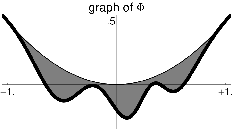
Figure 4: Potentials Φ\Phi with front parabolas for the examples from Figure 3 (top row) and 5 (bottom row).
Refer to caption
Refer to caption
Refer to caption
Refer to caption
Figure 5: Three counterexamples for the existence of action minimizing fronts. The first two examples satisfy the macroscopic constraints but violate the graph condition (G), so the iteration minimizes the action via an extending plateau. The third example violates the constraint Φ⁡(+1)=Φ⁡(−1)\Phi{\left({+1}\right)}=\Phi{\left({-1}\right)}, so the profiles converge to one of the asymptotic states.

In numerical simulations, the resulting iteration scheme has good convergence properties and decreases the action provided that λ{\lambda} is sufficiently small and LL is sufficiently large. Three examples with normalized front data and Φ\Phi as in Assumption 5 are shown in Figure 3, where Φ′\Phi^{\prime} is always plotted over the invariant interval [−Γ,Γ][-{\Gamma},\,{\Gamma}]. For plots of Φ\Phi see Figure 4. In the first example Φ′\Phi^{\prime} is increasing in [−1,+1][-1,\,+1] and the front profile WW turns out to be monotone. We refer to the remark at the end of §3 for an explanation, and to [HR09] for more examples. The other two examples in Figure 3 illustrate that the front profiles for non-convex Φ\Phi are in general non-monotone.


In order to illustrate the necessity of the graph condition (G) we present in Figure 5 simulations for potentials that violate this condition. In the first example the interval [−1, 1][-1,\,1] is invariant under Φ′\Phi^{\prime} but Ψ\Psi is negative in this interval. After some initial iterations the profiles exhibit an extending plateau at −1<w∗<1-1<w_{\ast}<1, where w∗w_{\ast} is the minimizer of Ψ\Psi in [−1, 1][-1,\,1] and satisfies w∗=Φ′​(w∗)w_{\ast}=\Phi^{\prime}{\left({w_{\ast}}\right)}. The onset of the extending plateau is a direct consequence of the energy landscape of ℒ\mathcal{L}, see Remark 12. The second simulation provides another counterexample for the existence of action minimizing fronts. Here Ψ\Psi has the correct sign close to ±1\pm 1 but attains again a negative minimum in −1<w∗<1-1<w_{\ast}<1. As before, the profiles minimize their action by converging to the ‘global minimizer’ W≡w∗W\equiv{w_{\ast}}. Finally, the third example illustrates what happens if the asymptotic states violate the macroscopic constraints. More precisely, here we violate (10) due to Φ⁡(+1)>Φ⁡(−1)\Phi{\left({+1}\right)}>\Phi{\left({-1}\right)}, and observe that the profiles converge to the global minimizer W≡+1W\equiv+1.

Acknowledgements

References

  • [AP07] S. Aubry and L. Proville, Pressure Fronts in 1D Nonlinear Lattices, to appear in proceedings of EQUADIFF-07, 2007.
  • [BCS01a] A.M. Balk, A. Cherkaev, and L. Slepyan, Dynamics of chains with non-monotone stress-strain relations. I. Model and numerical experiments, J. Mech. Phys. Solids 49 (2001), 131–148.
  • [BCS01b]   , Dynamics of chains with non-monotone stress-strain relations. II. Nonlinear waves and waves of phase transition, J. Mech. Phys. Solids 49 (2001), 149–171.
  • [DHM06] W. Dreyer, M. Herrmann, and A. Mielke, Micro-macro transition for the atomic chain via Whitham’s modulation equation, Nonlinearity 19 (2006), no. 2, 471–500.
  • [FM02] G. Friesecke and K. Matthies, Atomic-scale localization of high-energy solitary waves on lattices, Physica D 171 (2002), 211–220.
  • [FPU55] E. Fermi, J. Pasta, and S. Ulam, Studies on nonlinear problems, Los Alamos Scientific Laboraty Report LA–1940, 1955, reprinted in: D.C. Mattis (editor), The many body problem. World Scientific, 1993.
  • [FV99] A.-M. Filip and S. Venakides, Existence and modulation of traveling waves in particle chains, Comm. Pure Appl. Math. 51 (1999), no. 6, 693–735.
  • [FW94] G. Friesecke and J.A.D. Wattis, Existence theorem for solitary waves on lattices, Comm. Math. Phys. 161 (1994), no. 2, 391–418.
  • [Her09] M. Herrmann, Unimodal wave trains and solitons in convex FPU chains, preprint, see arXiv:0901.3736, 2009.
  • [HR09] M. Herrmann and J. Rademacher, Heteroclinic travelling waves in convex FPU-type chains, preprint, see arXiv:0812.1712, 2009.
  • [HR10] M. Herrmann and J. D. M. Rademacher, Riemann solvers and undercompressive shocks of convex FPU chains, Nonlinearity 23 (2010), no. 2, 277–304.
  • [IJ05] G. Iooss and G. James, Localized waves in nonlinear oscillator chains, Chaos 15 (2005), 015113.
  • [Ioo00] G. Iooss, Travelling waves in the Fermi-Pasta-Ulam lattice, Nonlinearity 13 (2000), 849–866.
  • [KZ09a] C.F. Kreiner and J. Zimmer, Heteroclinic travelling waves for the lattice sine-Gordon equation with linear pair interaction, Discrete Contin. Dyn. Syst. Ser. A 25 (2009), no. 3, 915–931.
  • [KZ09b]   , Travelling wave solutions for the discrete sine-Gordon equation with nonlinear pair interaction, Nonlinear Anal.-Theory Methods Appl. 70 (2009), no. 9, 3146–3158.
  • [Pan05] A. Pankov, Traveling Waves and Periodic Oscillations in Fermi-Pasta-Ulam lattices, Imperial College Press, London, 2005.
  • [PP00] A. Pankov and K. Pflüger, Traveling Waves in Lattice Dynamical Systems, Math. Meth. Appl. Sci. 23 (2000), 1223–1235.
  • [SCC05] L. Slepyan, A. Cherkaev, and E. Cherkaev, Transition waves in bistable structures. II. Analytical solution: wave speed and energy dissipation, J. Mech. Phys. Solids 53 (2005), 407–436.
  • [SW97] D. Smets and M. Willem, Solitary waves with prescribed speed on infinite lattices, J. Funct. Anal. 149 (1997), 266–275.
  • [SZ07] H. Schwetlick and J. Zimmer, Solitary waves for nonconvex FPU lattices, J. Nonlinear Sci. 17 (2007), no. 1, 1–12.
  • [SZ09]   , Existence of dynamic phase transitions in a one-dimensional lattice model with piecewise quadratic interaction potential, SIAM J. Math. Anal. 41 (2009), no. 3, 1231–1271.
  • [TV05] L. Truskinovsky and A. Vainchtein, Kinetics of martensitic phase transitions: lattice model, SIAM J. Appl. Math. 66 (2005), 533–553.
  • [Vai10] A. Vainchtein, The role of spinodal region in the kinetics of lattice phase transitions, J. Mech. Phys. Solids 58 (2010), no. 2, 227–240.