跳到论文正文
W Papers独立论文阅读器 arXiv:1002.0207 论文正文 计算阅读时间 · 0%
引用这篇论文根据当前论文元数据生成,正式投稿前建议核对。


License: arXiv.org perpetual non-exclusive license
arXiv:1002.0207v2 [cond-mat.mes-hall] 28 Apr 2010

Theory of spin relaxation torque in metallic ferromagnets

Noriyuki Nakabayashi, Akihito Takeuchi, Kazuhiro Hosono, Katsuhisa Taguchi, Gen Tatara Affiliation:  Department of Physics, Tokyo Metropolitan University, Hachioji, Tokyo 192-0397, Japan
August 24, 2026
Abstract

Spin transport driven by an external electric field in uniform metallic ferromagnets with the spin-orbit interaction arising from random impurities is studied microscopically. Spin relaxation torque 𝒯{\cal T} is shown to be written by spatial derivatives of the electric field, but with anisotropy arising from the magnetization. The field-driven contribution of the spin current is also anisotropic. The diffusive spin current is shown to be written as a gradient of the spin chemical potential, and the linear-response expression for the spin chemical potential is derived. It is discussed that the β\beta term in the spin transfer torque can also be anisotropic.

pacs
72.10.Bg 72.25.Rb

I Introduction

Spintronics aims at using the information carried by the electrons’ spin in solids. For this purpose, establishing reliable methods to create, transfer and detect the spin current is an urgent task. Compared to the charge transports, spin transports have one serious fundamental difficulty. That is the non-conservation of the spin in solids. This limits the range of the spin transmission to be less than the spin diffusion length, which is typically μ\mum scale in metals.

The non-conservation of the spins is expressed by a source term in the continuity equation for the spin

s˙α+∇⋅𝒋sα=𝒯α.\displaystyle\dot{s}^{\alpha}+\nabla\cdot\bm{j}_{\rm s}^{\alpha}={\cal T}^{\alpha}. (1)

Here ss and 𝒋s\bm{j}_{\rm s} are the spin density and spin current, respectively, α=x,y,z\alpha=x,y,z is the spin direction and 𝒯{\cal T} is the spin relaxation torque resulting in the non-conservation of the spin. In the most cases in metals, the dominant origin of 𝒯{\cal T} is the spin-orbit interaction.

Although the relaxation torque term is essential in spin transports, it has so far been treated only on the phenomenological ground. The continuity equation is equivalent to the Boltzmann equation, which is useful in discussing the spin transports. The Boltzmann equation for the distribution function of each spin channel was discussed by Son et al. [1] and later by Valet and Fert [2] in the context of the giant magnetoresistance in multilayer systems. In their analysis, they approximated the spin relaxation torque as proportional to the inverse of a spin relaxation time τsf\tau_{\rm sf} and to some unknown function representing a driving force for the spin accumulation. The driving force was written in terms of what they called the spin chemical potential μs\mu_{\rm s}. The relaxation torque was approximated as 𝒯z=μs/τsf{\cal T}^{z}=\mu_{\rm s}/\tau_{\rm sf}. They argued that μs\mu_{\rm s} satisfies the diffusion equation, ∇2μs=−ℓsf−2​μs\nabla^{2}\mu_{\rm s}=-\ell_{\rm sf}^{-2}\mu_{\rm s}, with the diffusion length ℓsf∝τsf\ell_{\rm sf}\propto\sqrt{\tau_{\rm sf}}. Microscopic calculation for μs\mu_{\rm s} has not been done so far.

The diffusion equation for the spin has been widely used to discuss recent spin transports in metallic junctions [3]. The decay of spin transport has been confirmed in non-local spin injection experiments [4, 5, 6], which indicate that the spin diffusion decays with a decay length of 350-500nm in Cu and 100nm in Au at room temperature. Although the spin diffusion equation appears to be so far successful, the phenomenological treatment of the spin relaxation term and the spin chemical potential must be improved to consider the spin transport seriously.

Besides diffusive spin current, there is another spin current that is driven by an effective field. In contrast to the diffusive one, this field-driven contribution should not decay in uniform (single domain) ferromagnets, since the ratio of the spin current and the charge current is determined by the spin polarization ratio of the material, which is a statistical mechanical quantity. The field-driven (local) spin current and the diffusive spin current behave differently, as was recently demonstrated theoretically in the case of the inverse spin Hall effect [7].

In the field of the current-driven magnetization dynamics, the spin relaxation torque has been studied from the microscopic viewpoint [8, 9, 10]. In this context, Eq. (1) gives the expression for the torque acting on the spin density 𝒔{{\bm{s}}} as

τα=−∇⋅𝒋sα+𝒯α.\displaystyle\tau^{\alpha}=-\nabla\cdot\bm{j}_{\rm s}^{\alpha}+{\cal T}^{\alpha}. (2)

In the adiabatic limit, i.e., slowly varying magnetization, and under uniform current, the first term reduces to ∇⋅𝒋sα=(P/2e)(𝒋⋅∇)𝒔α\nabla\cdot\bm{j}_{\rm s}^{\alpha}=(P/2e)(\bm{j}\cdot\nabla){{\bm{s}}}^{\alpha}, where PP is the spin polarization of the current [9, 10], namely to the adiabatic spin-transfer torque. When the spin-relaxation sets in, the conduction electron no longer follows the magnetization profile, and new contribution to the torque arises from the 𝒯{\cal T} term. This torque was shown to be

𝒯=−βPe​s2(𝒔×(𝒋⋅∇)𝒔),\displaystyle{\cal T}=-\beta\frac{P}{es^{2}}({{\bm{s}}}\times(\bm{j}\cdot\nabla){{\bm{s}}}), (3)

where β\beta is a coefficient inversely proportional to the spin relaxation time τs\tau_{\rm s} [8, 10]. This torque, called β\beta term, turned out to be essential in determining the efficiency of the current-driven domain wall motion [11, 12, 13]. The magnitude of the parameter β\beta has recently been intensively studied experimentally by measuring the domain wall speed under current [14, 15]. Theoretical formulation for estimating β\beta in the first-principles calculations was carried out recently [16].

The spin relaxation torque has been studied also from the viewpoint of how to define the spin current. It was discussed that the spin relaxation torque contains a term written as a divergence of the torque dipole density, 𝑷{\bm{P}} [17]. Generalized argument was given by Shi et al. [18], where they discussed that the zz component of the relaxation torque is written as a divergence,

𝒯z=−∇⋅𝑷,\displaystyle{\cal T}^{z}=-\nabla\cdot{\bm{P}}, (4)

if the system has the inversion symmetry. This means that the total torque integrated over the system should vanish. Shi et al. also argued that if the relaxation torque is a divergence of 𝑷{\bm{P}}, one can define a spin current that is conserved. In fact, defining 𝒋s~≡𝒋s+𝑷\tilde{\bm{j}_{\rm s}}\equiv\bm{j}_{\rm s}+{\bm{P}}, the continuity equation (1) reduces to s˙z+∇⋅𝒋s~=0\dot{s}^{z}+\nabla\cdot\tilde{\bm{j}_{\rm s}}=0. The explicit form of the torque dipole density was not calculated in Ref. [18]. Obviously, in the presence of the inhomogeneity of the magnetization, the β\beta torque (Eq. (3)) cannot be written as a divergence, and thus it indeed represents the spin angular momentum lost by the spin relaxation.

The result that the spin relaxation torque is given by a derivative of the applied electric field 𝑬{\bm{E}} is understood as follows. The spin relaxation torque should of course vanish when 𝑬=0{\bm{E}}=0. It cannot be directly proportional to 𝑬{\bm{E}}, since field-driven spin current in uniform ferromagnets should not decay. Therefore, the simplest expression for the relaxation torque is a derivative of the field. It is not, however, obvious whether it should be always written in a rotationally invariant way, or if it can be anisotropic, since the rotational invariance is broken in uniform ferromagnets because of the magnetization.

The first aim of the present paper is to calculate the spin relaxation torque microscopically in the presence of the applied electric field. The spin relaxation mechanism we take into account is the spin-orbit interaction due to random impurities. Our explicit calculation reveals that the spin relaxation torque is not always rotationally symmetric in uniform ferromagnets, but is generally given by

𝒯z=γ⁡(∇⋅𝑬)+δ​γ​(∂zEz),\displaystyle{\cal T}^{z}=\gamma(\nabla\cdot{\bm{E}})+\delta\gamma(\partial_{z}E_{z}), (5)

where zz axis is along the magnetization, γ\gamma and δ​γ\delta\gamma are coefficient proportional to the inverse spin relaxation time. The spin relaxation torque is, therefore, anisotropic. Relaxation torque of Eq. (5) indicates that the torque dipole density is given by

𝑷=−(γ​𝑬+δ​γ​(𝒏⋅𝑬)​𝒏),\displaystyle{\bm{P}}=-(\gamma{\bm{E}}+\delta\gamma({\bm{n}}\cdot{\bm{E}}){\bm{n}}), (6)

where 𝒏{\bm{n}} represents the direction of the magnetization. These anisotropic behaviors of the transport quantities is common when spin-orbit interaction exists, as is well-known in charge transport as the anisotropic magnetoresistance (AMR) [19].

The second aim of the paper is to study the spin current on the same microscopic footing as the relaxation torque. We show that the spin current is made up of a field-driven contribution which is local and the diffusive one with nonlocality. The field-driven contribution is anisotropic like the AMR effect for the charge current (we call the effect as spin AMR effect). The diffusive contribution is given as a gradient of a spin chemical potential, μs\mu_{\rm s}. We will derive the linear-response expression for the spin chemical potential. Our microscopic study on the spin current demonstrates the validity of the half-phenomenological treatments [2].

II Model

We consider the conduction electron system taking account of the spin-orbit interaction, the impurity scattering without spin flip, and the applied electric field. The Hamiltonian of the system is given as H=H0+Hso+Hem+HimpH=H_{0}+{H_{\rm so}}+H_{\rm em}+H_{\rm imp}, where H0H_{0} is the free electron Hamiltonian including the uniform magnetization, Hso{H_{\rm so}} is the spin-orbit interaction, HemH_{\rm em} is the interaction with the gauge field representing the applied electric field, and HimpH_{\rm imp} is the spin-independent impurity scattering. The free part reads

H0≡∑𝒌​σϵ𝒌​σ​c𝒌​σ†​c𝒌​σ,\displaystyle H_{0}\equiv\sum_{{\bm{k}}\sigma}\epsilon_{{\bm{k}}\sigma}c^{\dagger}_{{\bm{k}}\sigma}c_{{\bm{k}}\sigma}, (7)

where the electron creation and annihilation operators are denoted by c†{c^{\dagger}} and cc, respectively, ϵ𝒌​σ≡k22​m−ϵF−σ​M\epsilon_{{\bm{k}}\sigma}\equiv\frac{k^{2}}{2m}-{\epsilon_{F}}-\sigma{M}, ϵF{\epsilon_{F}} is the Fermi energy, M{M} is the spin splitting due to the magnetization and σ≡±\sigma\equiv\pm represents the spin. The spin-orbit interaction is represented by Hso=Hso0+HsoA{H_{\rm so}}={H_{\rm so}}^{0}+{H_{\rm so}}^{A}, where (σk\sigma_{k} (k=x,y,zk=x,y,z) is the Pauli matrix)

Hso0\displaystyle{H_{\rm so}}^{0} =−i2∑i​j​kϵi​j​k∫d3x(∇ivso(k))(c†∇j↔σkc)\displaystyle=-\frac{i}{2}\sum_{ijk}\epsilon_{ijk}\int\!{d^{3}x}(\nabla_{i}v_{\rm so}^{(k)})({c^{\dagger}}\stackrel{{\scriptstyle{\leftrightarrow}}}{{\nabla}}_{j}\sigma_{k}c) (8)
HsoA\displaystyle{H_{\rm so}}^{A} =−e∑i​j​kϵi​j​k∫d3x(∇ivso(k))Aj(𝒙,t)(c†σkc).\displaystyle=-e\sum_{ijk}\epsilon_{ijk}\int\!{d^{3}x}(\nabla_{i}v_{\rm so}^{(k)})A_{j}({\bm{x}},t)({c^{\dagger}}\sigma_{k}c). (9)

(We suppress the spin index when obvious, namely, c=(c+,c−)c=(c_{+},c_{-}). ) The spin-orbit potential vso(k)v_{\rm so}^{(k)} is assumed to arise from random impurities and to depend on the spin direction (kk). The averaging over the spin-orbit potential is carried out as

⟨vso(k)​(𝒑)​vso(γ)​(−𝒑′)⟩i=nso​λso2​δ𝒑,𝒑′​δk​γ,\displaystyle\left\langle{v_{\rm so}^{(k)}({\bm{p}})v_{\rm so}^{(\gamma)}(-{\bm{p}}^{\prime})}\right\rangle_{\rm i}=n_{{\rm so}}{\lambda_{\rm so}}^{2}\delta_{{\bm{p}},{\bm{p}}^{\prime}}\delta_{k\gamma}, (10)

where nson_{{\rm so}} and λso{\lambda_{\rm so}} are the concentration of the spin-orbit impurities and the strength of the interaction, respectively. The average of the spin-orbit potential at the linear order is zero in our model, and thus we do not take account of the the anomalous Hall and spin Hall effects. We consider a case where electric field 𝑬⁡(𝒙,t)(≡−𝑨˙​(𝒙,t)){\bm{E}}({\bm{x}},t)(\equiv-\dot{{\bm{A}}}({\bm{x}},t)) is position and time dependent. The electromagnetic interaction is written as

Hem=−em∑𝒌,𝒒∑ikiAi(𝒒,Ω)(c†𝒌−𝒒2c𝒌+𝒒2),\displaystyle H_{\rm em}=-\frac{e}{m}\sum_{{\bm{k}},{\bm{q}}}\sum_{i}k_{i}A_{i}({\bm{q}},\Omega)({c^{\dagger}}_{{{\bm{k}}}-\frac{{\bm{q}}}{2}}c_{{{\bm{k}}}+\frac{{\bm{q}}}{2}}), (11)

where Ω\Omega is the frequency of the electric field. We will consider the limit of small Ω\Omega and small qq. The scattering by the normal impurities is represented by

Himp\displaystyle H_{\rm imp} =∑i=1Nimp∑𝒌​𝒌′viN​ei⁡(𝒌−𝒌′)⋅𝑹i​c†𝒌′​c𝒌,\displaystyle=\sum_{i=1}^{N_{\rm imp}}\sum_{{\bm{k}}{\bm{k}}^{\prime}}\frac{v_{\rm i}}{N}e^{i({\bm{k}}-{\bm{k}}^{\prime})\cdot{\bm{R}}_{i}}{c^{\dagger}}_{{\bm{k}}^{\prime}}c_{{\bm{k}}}, (12)

where viv_{\rm i} represents the strength of the impurity potential, 𝑹i{\bm{R}}_{i} represents the position of random impurities, NimpN_{\rm imp} is the number of impurities, and N≡V/a3N\equiv V/a^{3} is number of sites. To estimate physical quantities, we take the random average over impurity positions in a standard manner [9].

To derive the spin continuity equation, Eq. (1), we derive the equation of motion for the spin density, 𝒔⁡(𝒙,t)≡⟨c†​(𝒙,t)​𝝈​c​(𝒙,t)⟩{\bm{{s}}}({\bm{x}},t)\equiv\left\langle{{c^{\dagger}}({\bm{x}},t){\bm{\sigma}}c({\bm{x}},t)}\right\rangle (⟨⟩\left\langle{\ }\right\rangle represents the quantum average). The time development of the spin density reads

s˙α\displaystyle\dot{s}^{\alpha} =i⁡⟨[H,c†]​σα​c+c†​σα​[H,c]⟩,\displaystyle=i\left\langle{[H,c^{\dagger}]\sigma^{\alpha}c+c^{\dagger}\sigma^{\alpha}[H,c]}\right\rangle, (13)

where HH is the total Hamiltonian of the system. The commutators are calculated as in Appendix A, and Eq. (13) turns out to be Eq. (1), namely

s˙α=−∇⋅𝒋sα+𝒯α,\displaystyle\dot{s}^{\alpha}=-\nabla\cdot\bm{j}_{\rm s}^{\alpha}+{\cal T}^{\alpha},

with the spin current given as

jsα≡js(n),α+jsso,α,\displaystyle j_{\rm s}^{\alpha}\equiv j_{\rm s}^{{\rm(n)},\alpha}+j_{\rm s}^{{\rm so},\alpha}, (14)

where

js,i(n),α\displaystyle j_{{\rm s},i}^{{\rm(n)},\alpha} ≡−i2​m⟨c†σα∇i↔c⟩−emAi⟨c†σαc⟩\displaystyle\equiv-\frac{i}{2m}\left\langle{{c^{\dagger}}\sigma^{\alpha}\stackrel{{\scriptstyle{\leftrightarrow}}}{{\nabla}}_{i}c}\right\rangle-\frac{e}{m}A_{i}\left\langle{{c^{\dagger}}\sigma_{\alpha}c}\right\rangle
≡js,i(0),α+js,iA,α,\displaystyle\equiv j_{{\rm s},i}^{(0),\alpha}+j_{{\rm s},i}^{A,\alpha}, (15)

and

js,iso,α≡−∑jϵi​j​α(∇jvso(α))⟨c†c⟩.\displaystyle j_{{\rm s},i}^{{\rm so},\alpha}\equiv-\sum_{j}\epsilon_{ij\alpha}(\nabla_{j}v_{\rm so}^{(\alpha)})\left\langle{{c^{\dagger}}c}\right\rangle. (16)

The relaxation torque reads

𝒯α≡𝒯soα+𝒯soA,α,\displaystyle{\cal T}^{\alpha}\equiv{\cal T}_{{\rm so}}^{\alpha}+{\cal T}_{{\rm so}}^{A,\alpha}, (17)

where

𝒯soα\displaystyle{\cal T}_{{\rm so}}^{\alpha} ≡i∑i​j​k​lϵi​j​kϵα​l​k(∇ivso(k))⟨c†σl∇j↔c⟩,\displaystyle\equiv i\sum_{ijkl}\epsilon_{ijk}\epsilon_{\alpha lk}(\nabla_{i}v_{\rm so}^{(k)})\left\langle{{c^{\dagger}}\sigma_{l}\stackrel{{\scriptstyle{\leftrightarrow}}}{{\nabla}}_{j}c}\right\rangle, (18)
𝒯soA,α\displaystyle{\cal T}_{{\rm so}}^{A,\alpha} ≡2​e​∑i​j​k​lϵi​j​k​ϵα​l​k​(∇ivso(k))​Aj​⟨c†​σl​c⟩.\displaystyle\equiv 2e\sum_{ijkl}\epsilon_{ijk}\epsilon_{\alpha lk}(\nabla_{i}v_{\rm so}^{(k)})A_{j}\left\langle{{c^{\dagger}}\sigma_{l}c}\right\rangle. (19)

The spin relaxation torque depends on the definition of the spin current. For instance, if we redefine the spin current as 𝒋s′α≡𝒋sα−𝑪α{\bm{j}_{\rm s}^{\prime}}^{\alpha}\equiv{\bm{j}_{\rm s}^{\alpha}}-{\bm{C}}^{\alpha}, where 𝑪{\bm{C}} is a vector, the continuity equation (1) becomes s˙α+∇⋅𝒋s′α=𝒯′α\dot{s}^{\alpha}+\nabla\cdot{\bm{j}_{\rm s}^{\prime}}^{\alpha}={{\cal T}^{\prime}}^{\alpha}, where the relaxation torque reads 𝒯′α≡𝒯α+∇⋅𝑪α{{\cal T}^{\prime}}^{\alpha}\equiv{{\cal T}}^{\alpha}+\nabla\cdot{\bm{C}}^{\alpha}. This ambiguity of spin current definition of course does not affect physical quantities such as the total torque acting on the spin density, which is given by 𝒔˙\dot{{{\bm{s}}}}.

III Spin relaxation torque

We calculate the spin relaxation torque as a linear response to the applied electric field. The uniform magnetization is chosen as along zz axis. The spin-orbit interaction is included to the second order.

Refer to caption
Figure 1: Feynman diagrams representing the relaxation torque. Solid lines represent the electron Green’s function with the lifetime (τσ\tau_{\sigma}) included, vsov_{\rm so} represents the spin-orbit interaction (double dashed line) and dotted line represents the interaction with the gauge field (AA). The first two diagrams are the contributions to 𝒯soα{\cal T}_{{\rm so}}^{\alpha} and the last diagram is the contribution to 𝒯soA,α{\cal T}_{{\rm so}}^{A,\alpha}. The vertex marked by cross represents the relaxation torque.

The contributions to the relaxation torque, Eq. (17), are shown in Fig. 1. The leading contribution for small 1/(ϵF​τ)1/({\epsilon_{F}}\tau) and q​ℓq\ell (ℓ\ell is the electron mean free path) turns out to be the first diagram in Fig. 1, which reads (see Appendix B for details)

𝒯α\displaystyle{\cal T}^{\alpha} =δα,z245​πnsoλso2em2(3∇⋅𝑨˙+∇zA˙z)\displaystyle=\delta_{\alpha,z}\frac{2}{45\pi}n_{{\rm so}}{\lambda_{\rm so}}^{2}\frac{e}{m^{2}}(3\nabla\cdot\dot{{\bm{A}}}+\nabla_{z}\dot{A}_{z})
×∑𝒌​𝒌′k2(k′)4∑σ=±σg𝒌,σrg𝒌′,−σr(g𝒌′,−σa)2+c.c.,\displaystyle\times\sum_{{\bm{k}}{\bm{k}}^{\prime}}k^{2}(k^{\prime})^{4}\sum_{\sigma=\pm}\sigma g_{{\bm{k}},\sigma}^{{\rm r}}g_{{\bm{k}}^{\prime},-\sigma}^{{\rm r}}(g_{{\bm{k}}^{\prime},-\sigma}^{{\rm a}})^{2}+{\rm c.c.}, (20)

where g𝒌​σrg_{{\bm{k}}\sigma}^{{\rm r}} and g𝒌​σag_{{\bm{k}}\sigma}^{{\rm a}} are the retarded and advanced electron Green’s functions, respectively, carrying the wave vector 𝒌{\bm{k}} and spin σ\sigma with zero frequency. As we see, only zz component of the torque is finite. The Green’s functions include the lifetime arising from the self-energy process due to normal impurities and the spin-orbit interaction. The inverse lifetime for the electron with spin σ(=±)\sigma(=\pm) is given as

τσ−1=2​π​ni​vi2​νσ​(1+κz,σ+κ⟂​γσ),\displaystyle{\tau_{\sigma}}^{-1}=2\pi n_{\rm i}v_{\rm i}^{2}\nu_{\sigma}(1+\kappa_{z,\sigma}+\kappa_{\perp}\gamma_{\sigma}), (21)

where νσ\nu_{\sigma} is the spin-resolved electron density of states, nin_{\rm i} and viv_{\rm i} are the concentration and the potential strength of the impurities, κz,σ≡13​nso​λso2ni​vi2​kF​σ4\kappa_{z,\sigma}\equiv\frac{1}{3}\frac{n_{{\rm so}}{\lambda_{\rm so}}^{2}}{n_{\rm i}v_{\rm i}^{2}}k_{F\sigma}^{4} and κ⟂≡23​nso​λso2ni​vi2​kF+2​kF−2\kappa_{\perp}\equiv\frac{2}{3}\frac{n_{{\rm so}}{\lambda_{\rm so}}^{2}}{n_{\rm i}v_{\rm i}^{2}}k_{F+}^{2}k_{F-}^{2} are dimensionless ratios of the spin-orbit interaction to the normal impurity scattering (kF​σk_{F\sigma} is the spin-dependent Fermi wavelength), and γσ≡ν−σνσ\gamma_{\sigma}\equiv\frac{\nu_{-\sigma}}{\nu_{\sigma}}. The total relaxation torque is therefore given by (Eq. (5)),

𝒯z=γ⁡(∇⋅𝑬)+δ​γ​(∂zEz),\displaystyle{\cal T}^{z}=\gamma(\nabla\cdot{\bm{E}})+\delta\gamma(\partial_{z}E_{z}), (22)

where

γ\displaystyle\gamma ≡8​π​e15​m2nsoλso2ν+ν−kF+2kF−2∑σ=±σkF​σ2τσ2\displaystyle\equiv\frac{8\pi e}{15m^{2}}n_{{\rm so}}{\lambda_{\rm so}}^{2}\nu_{+}\nu_{-}k_{F+}^{2}k_{F-}^{2}\sum_{\sigma=\pm}\sigma k_{F\sigma}^{2}\tau_{\sigma}^{2} (23)

and δ​γ≡γ/3\delta\gamma\equiv\gamma/3. The parameter γ\gamma is proportional to the spin flip rate due to the spin-orbit interaction. Our result indicates that the relaxation torque is zero in uniform ferromagnet when uniform electric field is applied. Thus the spin current does not decay in this case. In fact, the static solution of Eq. (1) with 𝒯z=0{\cal T}^{z}=0 is jsz=constantj_{\rm s}^{z}={\rm constant}.

The degree of the asymmetry, δ​γ/γ\delta\gamma/\gamma, is not universal but is model dependent. For instance, in the case of junction with weak electron hopping at point-like leads, δ​γ\delta\gamma vanishes [20].

IV Spin current

We here calculate the spin current within the same formalism. Within the linear response theory, the spin current is calculated by estimating the Feynman diagrams shown in Figs. 2 and 3, which correspond to the field-induced contribution and the effect of the diffusive electron motion, respectively.

Refer to caption
Figure 2: Feynman diagrams representing the local contribution to the spin current (the first two terms in Eq. (37)). The first three diagrams correspond to js(n)j_{{\rm s}}^{{\rm(n)}}, and the last two diagrams represent the contribution from the anomalous velocity, jssoj_{{\rm s}}^{{\rm so}}. Dotted and double dashed lines denote the interaction with the applied electric field and the spin-orbit interaction, respectively. The vertex marked by cross represents the spin current.
Refer to caption
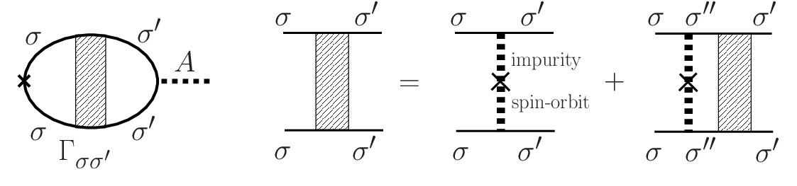
Figure 3: Left: The vertex correction contribution to js(n),zj_{\rm s}^{{\rm(n)},z}, resulting in the diffusive spin current (the last term of Eq. (37)). Right: Γσ​σ′\Gamma_{\sigma\sigma^{\prime}}, which is a ladder process of the successive electron scattering by the normal impurity and the spin-orbit interaction (represented by thick dotted lines) connecting the spin indices σ\sigma and σ′\sigma^{\prime}.

We first estimate the normal part of the spin current, js,i(n),zj_{{\rm s},i}^{{\rm(n)},z} (Eq. (15)), shown in the first two diagrams in Fig. 2. The contribution js,i(n),zj_{{\rm s},i}^{{\rm(n)},z} is defined including the anomalous contribution from the electromagnetic gauge field, js,iA,zj_{{\rm s},i}^{A,z}. Its dominant contribution in the limit of small Ω\Omega and small qq is calculated as (see Appendix C for detail)

js,i(n),z\displaystyle j_{{\rm s},i}^{{\rm(n)},z} =−i12​πe2m2∑𝒌​𝒒e−i𝒒⋅𝒙∫d​Ω2​πei​Ω​t∑jΩAj(𝒒,Ω)∑σσ[kikjg𝒌−𝒒2,σrg𝒌+𝒒2,σa\displaystyle=-i\frac{1}{2\pi}\frac{e^{2}}{m^{2}}\sum_{{\bm{k}}{\bm{q}}}e^{-i{\bm{q}}\cdot{\bm{x}}}\int\!\frac{d\Omega}{2\pi}e^{i\Omega t}\sum_{j}\Omega A_{j}({\bm{q}},\Omega)\sum_{\sigma}\sigma\left[k_{i}k_{j}g_{{{\bm{k}}}-\frac{{\bm{q}}}{2},\sigma}^{{\rm r}}g_{{{\bm{k}}}+\frac{{\bm{q}}}{2},\sigma}^{{\rm a}}\right.
+∑𝒌′​σ′kikj′g𝒌−𝒒2,σrg𝒌+𝒒2,σag𝒌′−𝒒2,σ′rg𝒌′+𝒒2,σ′anivi2Γσ​σ′(𝒒,Ω)]\displaystyle\left.+\sum_{{\bm{k}}^{\prime}\sigma^{\prime}}k_{i}k^{\prime}_{j}g_{{{\bm{k}}}-\frac{{\bm{q}}}{2},\sigma}^{{\rm r}}g_{{{\bm{k}}}+\frac{{\bm{q}}}{2},\sigma}^{{\rm a}}g_{{{{\bm{k}}}^{\prime}}-\frac{{\bm{q}}}{2},\sigma^{\prime}}^{{\rm r}}g_{{{{\bm{k}}}^{\prime}}+\frac{{\bm{q}}}{2},\sigma^{\prime}}^{{\rm a}}n_{\rm i}v_{\rm i}^{2}\Gamma_{\sigma\sigma^{\prime}}({\bm{q}},\Omega)\right] (24)

In Eq. (24), the first term is the contribution shown in the left of Fig. 2, and the second term is the contribution from the vertex correction (Fig. 3).

The factor Γσ​σ′​(𝒒,Ω)\Gamma_{\sigma\sigma^{\prime}}({\bm{q}},\Omega) contains all the vertex corrections due to the normal impurities and the spin-orbit interaction shown in Fig. 3. The equation of motion for Γσ​σ′\Gamma_{\sigma\sigma^{\prime}} is derived in the same manner as in Ref. [21] carried out in the context of quantum correction (the diffusion without the spin-orbit interaction was considered in Ref. [22]). The equation is obtained as

Γσ​σ\displaystyle\Gamma_{\sigma\sigma} =(1+κz)​(1+Πσ​Γσ​σ)+κ⟂​Π−σ​Γ−σ,σ\displaystyle=(1+\kappa_{z})(1+\Pi_{\sigma}\Gamma_{\sigma\sigma})+\kappa_{\perp}\Pi_{-\sigma}\Gamma_{-\sigma,\sigma}
Γσ,−σ\displaystyle\Gamma_{\sigma,-\sigma} =κ⟂​(1+Π−σ​Γ−σ,−σ)+(1+κz)​Πσ​Γσ,−σ,\displaystyle=\kappa_{\perp}(1+\Pi_{-\sigma}\Gamma_{-\sigma,-\sigma})+(1+\kappa_{z})\Pi_{\sigma}\Gamma_{\sigma,-\sigma}, (25)

where

Πσ​(𝒒,Ω)\displaystyle\Pi_{\sigma}({\bm{q}},\Omega) ≡ni​vi2​∑𝒌g𝒌−𝒒2,σr​g𝒌+𝒒2,σa\displaystyle\equiv n_{\rm i}v_{\rm i}^{2}{\sum_{{\bm{k}}}}g_{{{\bm{k}}}-\frac{{\bm{q}}}{2},\sigma}^{{\rm r}}g_{{{\bm{k}}}+\frac{{\bm{q}}}{2},\sigma}^{{\rm a}}
≃[1−(Dσ​q2​τσ+κz+κ⟂​γσ)],\displaystyle\simeq[1-(D_{\sigma}q^{2}\tau_{\sigma}+\kappa_{z}+\kappa_{\perp}\gamma_{\sigma})], (26)

where Dσ≡(kF​σ)23​m2​τσD_{\sigma}\equiv\frac{(k_{F\sigma})^{2}}{3m^{2}}\tau_{\sigma} is the diffusion constant. Neglecting quantities of order of (κz,κ⟂)2(\kappa_{z},\kappa_{\perp})^{2}, Eq. (25) is solved as

Γσ​σ\displaystyle\Gamma_{\sigma\sigma} =1+κz−(1+2​κz)​Π−σ[1−(1+κz)​Π+]​[1−(1+κz)​Π−]\displaystyle=\frac{1+\kappa_{z}-(1+2\kappa_{z})\Pi_{-\sigma}}{[1-(1+\kappa_{z})\Pi_{+}][1-(1+\kappa_{z})\Pi_{-}]}
Γσ,−σ\displaystyle\Gamma_{\sigma,-\sigma} =κ⟂[1−(1+κz)​Π+]​[1−(1+κz)​Π−].\displaystyle=\frac{\kappa_{\perp}}{[1-(1+\kappa_{z})\Pi_{+}][1-(1+\kappa_{z})\Pi_{-}]}. (27)

Using Eq. (26), we obtain Γσ​σ′\Gamma_{\sigma\sigma^{\prime}} as (assuming the rotational symmetry for the wave vectors when averaging over the spin-orbit potential)

Γσ​σ\displaystyle\Gamma_{\sigma\sigma} =1Dσ​q2​τσ+κ⟂​γσ\displaystyle=\frac{1}{D_{\sigma}q^{2}\tau_{\sigma}+\kappa_{\perp}\gamma_{\sigma}}
Γσ,−σ\displaystyle\Gamma_{\sigma,-\sigma} =κ⟂[D+​q2​τ++κ⟂​γ+]​[D−​q2​τ−+κ⟂​γ−].\displaystyle=\frac{\kappa_{\perp}}{[D_{+}q^{2}\tau_{+}+\kappa_{\perp}\gamma_{+}][D_{-}q^{2}\tau_{-}+\kappa_{\perp}\gamma_{-}]}. (28)

By use of Eq. (28) and summing over the wave vectors, the normal spin current, Eq. (24), reads

js,i(n),z\displaystyle j_{{\rm s},i}^{{\rm(n)},z} =σs0​Ei−∇iμs,\displaystyle=\sigma_{{\rm s}}^{0}E_{i}-\nabla_{i}\mu_{\rm s}, (29)

where σs0≡e​∑±(±)​D±​ν±\sigma_{{\rm s}}^{0}\equiv e\sum_{\pm}(\pm)D_{\pm}\nu_{\pm} is the bare spin conductivity divided by ee. The first term of Eq. (29) is the field-driven contribution. The second gradient term is a diffusive contribution (vertex corrections), arising from the spin accumulation. The effective potential describing the spin accumulation, μs\mu_{\rm s}, reads

μs≡∫d3​x′​χ​(𝒙−𝒙′)​(∇⋅𝑬)​(𝒙′),\displaystyle\mu_{\rm s}\equiv\int\!{d^{3}x}^{\prime}\chi({\bm{x}}-{\bm{x}}^{\prime})(\nabla\cdot{\bm{E}})({\bm{x}}^{\prime}), (30)

where χ\chi is a correlation function arising from the electron diffusion, given as (VV is the system volume)

χ⁡(𝒙)\displaystyle\chi({\bm{x}}) ≡−∑±(±)σ±1V∑𝒒e−i𝒒⋅𝒙q2+(ℓs,±)−2.\displaystyle\equiv-\sum_{\pm}(\pm)\sigma_{\pm}\frac{1}{V}{\sum_{{\bm{q}}}}\frac{e^{-i{\bm{q}}\cdot{\bm{x}}}}{q^{2}+(\ell_{{\rm s},\pm})^{-2}}. (31)

Here σ±≡e​D±​ν±\sigma_{\pm}\equiv eD_{\pm}\nu_{\pm} is the spin-resolved Boltzmann conductivity divided by ee, and the correlation length is given as

ℓs,σ=Dσ​τs,σ.\displaystyle\ell_{{\rm s},\sigma}=\sqrt{D_{\sigma}\tau_{{\rm s},\sigma}}. (32)

The lifetime of the spin σ\sigma electron reads τs,σ≡τσ/(κ⟂​γσ)\tau_{{\rm s},\sigma}\equiv{\tau_{\sigma}}/{(\kappa_{\perp}\gamma_{\sigma})}. Defining μs=μ+−μ−\mu_{\rm s}=\mu_{+}-\mu_{-}, we see that spin-resolved effective potential satisfies

(−∇2+(ℓs,σ)−2)​μσ=−σσ​(∇⋅𝑬).\displaystyle(-\nabla^{2}+(\ell_{{\rm s},\sigma})^{-2})\mu_{\sigma}=-\sigma_{\sigma}(\nabla\cdot{\bm{E}}). (33)

In three-dimensions, the correlation function reads

χ(𝒙)=14​π​|𝒙|∑±(±)σ±e−|𝒙|/ℓs,±.\displaystyle\chi({\bm{x}})=\frac{1}{4\pi|{\bm{x}}|}\sum_{\pm}(\pm){\sigma_{\pm}}e^{-|{\bm{x}}|/\ell_{{\rm s},\pm}}. (34)

The local part of the spin current arises also from the anomalous spin current due to the spin-orbit interaction, defined in Eq. (16). This contribution is calculated by evaluating the last two diagrams in Fig. 2 as (see Appendix C)

js,iso,z\displaystyle j_{{\rm s},i}^{{\rm so},z} =δ​σs​(1−δi,z)​Ei,\displaystyle=\delta\sigma_{{\rm s}}(1-\delta_{i,z})E_{i}, (35)

where

δ​σs\displaystyle\delta\sigma_{{\rm s}} ≡π9​nso​λso2​em​∑±(±)​(kF±)4​(ν±)2​τ±.\displaystyle\equiv\frac{\pi}{9}n_{{\rm so}}{\lambda_{\rm so}}^{2}\frac{e}{m}\sum_{\pm}(\pm)(k_{F\pm})^{4}(\nu_{\pm})^{2}\tau_{\pm}. (36)

This spin-orbit correction to the spin conductivity is anisotropic, resulting in a spin version of the anisotropic magnetoresistance (AMR) effect, namely, spin AMR effect.

From Eqs. (24)(28)(35), the leading contribution to the spin current for small 𝒒{\bm{q}} and Ω\Omega is obtained as the sum of the local part driven by the electric field and the diffusive part as

𝒋sz=σs​𝑬−δ​σs​(𝒏⋅𝑬)​𝒏−∇μs,\displaystyle\bm{j}_{{\rm s}}^{z}=\sigma_{{\rm s}}{\bm{E}}-\delta\sigma_{\rm s}({\bm{n}}\cdot{\bm{E}}){\bm{n}}-\nabla\mu_{\rm s}, (37)

where σs≡σs0+δ​σs\sigma_{{\rm s}}\equiv\sigma_{{\rm s}}^{0}+\delta\sigma_{{\rm s}} and 𝒏{\bm{n}} is the unit vector along the magnetization. In terms of the angle θ\theta defined by cos⁡θ≡(𝒏⋅𝑬)/E\cos\theta\equiv({\bm{n}}\cdot{\bm{E}})/E, the magnitude of the field-driven (local) current reads

jsloc,z=(σs∥)2+((σs⟂)2−(σs∥)2)sin2θ,\displaystyle j_{{\rm s}}^{{\rm loc},z}=\sqrt{(\sigma_{{\rm s}\parallel})^{2}+((\sigma_{{\rm s}\perp})^{2}-(\sigma_{{\rm s}\parallel})^{2})\sin^{2}\theta}, (38)

where σs∥≡σs0\sigma_{{\rm s}\parallel}\equiv\sigma_{{\rm s}}^{0} and σs⟂≡σs\sigma_{{\rm s}\perp}\equiv\sigma_{{\rm s}}. When the degree of the anisotropy is small, the spin current becomes

jsloc,zE=σs∥(1+12(σs⟂σs∥)2sin2θ).\displaystyle\frac{j_{{\rm s}}^{{\rm loc},z}}{E}=\sigma_{{\rm s}\parallel}\left(1+\frac{1}{2}\left(\frac{\sigma_{{\rm s}\perp}}{\sigma_{{\rm s}\parallel}}\right)^{2}\sin^{2}\theta\right). (39)

We define the magnitude of the spin AMR as

Δ​ρsρs⟂\displaystyle\frac{\Delta\rho_{{\rm s}}}{\rho_{{\rm s}\perp}} ≡ρs∥−ρs⟂ρs⟂=δ​σs/σs1−δ​σs/σs,\displaystyle\equiv\frac{\rho_{{\rm s}\parallel}-\rho_{{\rm s}\perp}}{\rho_{{\rm s}\perp}}=\frac{\delta\sigma_{{\rm s}}/\sigma_{{\rm s}}}{1-\delta\sigma_{{\rm s}}/\sigma_{{\rm s}}}, (40)

where ρs​α≡(σs​α)−1\rho_{{\rm s}\alpha}\equiv(\sigma_{{\rm s}\alpha})^{-1} (α=∥,⟂\alpha=\parallel,\perp).

V Spin injection

We have thus derived the explicit expression for the spin chemical potential within the linear response theory. Let us apply Eq. (30) to a ferromagnetic-normal metal junction with an insulating barrier, used in the nonlocal spin injection experiments [5], depicted in Fig. 4(a). When the voltage is applied perpendicular to the interface (we choose the xx axis in this direction), the electric field is uniform inside the ferromagnet and the normal metal except at the interface. Writing the voltage drop at the interface (chosen as at x=0x=0) by VFNV_{\rm FN}, we obtain

∇⋅𝑬≃δ⁡(x)​VFN/d,\displaystyle\nabla\cdot{\bm{E}}\simeq\delta(x)V_{\rm FN}/d, (41)

where dd is the width of the interaface, which is treated as small enough compared with the electron mean free path, resulting in the delta function in ∇⋅𝑬\nabla\cdot{\bm{E}}. In totally unpolarized non-magnetic metals, namely, if σ+=σ−\sigma_{+}=\sigma_{-} and D+=D−D_{+}=D_{-}, the correlation function in Eq. (31) always vanishes. As is naively guessed, therefore, spin injection thus requires an effective spin polarization close to the interface, induced by the exchange interaction with the ferromagnet. This spin polarization is expected to be localized within a short distance of a few lattice constants from the interface. Let us approximate the interface polarization by introducing spin-dependent diffusion constant and the density of states, D¯σ\overline{D}_{\sigma} and ν¯σ\overline{\nu}_{\sigma}, respectively, at the interface. The long-range behavior of the spin correlation function in the non-magnetic side is then obtained as

χ(N)​(𝒙)\displaystyle\chi^{\rm(N)}({\bm{x}}) =−e4​π​(∑σσ​D¯σ​ν¯σ)​e−|𝒙|/ℓs|𝒙|,\displaystyle=-\frac{e}{4\pi}(\sum_{\sigma}\sigma\overline{D}_{\sigma}\overline{\nu}_{\sigma})\frac{e^{-|{\bm{x}}|/\ell_{{\rm s}}}}{|{\bm{x}}|}, (42)

where ℓs\ell_{{\rm s}} in the spin diffusion length in the normal metal ( ℓs\ell_{{\rm s}} is a long (∼μ\sim\mum) length scale and thus does not depend on the spin). We therefore obtain from Eq. (30) the chemical potential as

μs(N)​(𝒙)\displaystyle\mu_{\rm s}^{\rm(N)}({\bm{x}}) =qs4​π​|𝒙|e−|𝒙|/ℓs,\displaystyle=\frac{q_{\rm s}}{4\pi|{\bm{x}}|}e^{-|{\bm{x}}|/\ell_{{\rm s}}}, (43)

where OPENqs≡(∑σσ​D¯σ​ν¯σ)​e​VFN)​AFN/dq_{\rm s}\equiv(\sum_{\sigma}\sigma\overline{D}_{\sigma}\overline{\nu}_{\sigma})eV_{\rm FN})A_{\rm FN}/d, is the spin accumulation rate at the interface (per unit time), and AFNA_{\rm FN} is the area of the junction. This result of μs\mu_{\rm s} is consistent with intuitive and phenomenological results of the spin injection in the perpendicular structure shown in Fig. 4(a). In contrast, when the voltage is applied parallel to the ideal interface as shown in Fig. 4(b), spin injection does not occur since ∇⋅𝑬=0\nabla\cdot{\bm{E}}=0 at the interaface and thus μs(N)=0\mu_{\rm s}^{\rm(N)}=0.

Refer to caption
Figure 4: (a) Creation of diffusive spin current (spin injection) by applying the electric voltage perpendicular to the F-N interface. (b) When the voltage is applied parallel to an ideal interface, no spin current is induced since ∇⋅𝑬=0\nabla\cdot{\bm{E}}=0.

VI Total torque and asymmetric β\beta term

The continuity equation (1), indicates that the spin polarization (magnetization) changes due to the spin relaxation. (Change of the magnetization magnitude is a feature of the itinerant magnetism.) By use of Eqs. (5)(33)(37), we see that Eq. (1) results in

s˙z\displaystyle\dot{s}^{z} =γτ∇⋅𝑬+δγτ∇zEz+∑±(±)μ±(ℓs,±)2,\displaystyle=\gamma_{\tau}\nabla\cdot{\bm{E}}+\delta\gamma_{\tau}\nabla_{z}E_{z}+\sum_{\pm}(\pm)\frac{\mu_{\pm}}{(\ell_{{\rm s},\pm})^{2}}, (44)

where γτ≡γ−δ​σs\gamma_{\tau}\equiv\gamma-\delta\sigma_{{\rm s}} and δ​γτ≡δ​γ+δ​σs\delta\gamma_{\tau}\equiv\delta\gamma+\delta\sigma_{{\rm s}}. General case with uniform magnetization along any unit vector 𝒏{\bm{n}} is given by (𝒔≡s​𝒏{{\bm{s}}}\equiv s{\bm{n}})

𝒔˙\displaystyle\dot{{{\bm{s}}}} =𝒏(γτ∇⋅𝑬+δγτ∇∥E∥+∑±(±)μ±(ℓs,±)2),\displaystyle={\bm{n}}\left(\gamma_{\tau}\nabla\cdot{\bm{E}}+\delta\gamma_{\tau}\nabla_{\parallel}E_{\parallel}+\sum_{\pm}(\pm)\frac{\mu_{\pm}}{(\ell_{{\rm s},\pm})^{2}}\right), (45)

where E∥≡𝒏⋅𝑬E_{\parallel}\equiv{\bm{n}}\cdot{\bm{E}} and ∇∥≡𝒏⋅∇\nabla_{\parallel}\equiv{\bm{n}}\cdot\nabla.

In addition to the change of the magnitude, Eq. (45), there is a torque, which is perpendicular to 𝒏{\bm{n}}. Such torque arises when the magnetization is not homogeneous, and plays important roles in current-induced magnetization dynamics. We have carried out the calculation of the current-induced torque done in Ref. [10] on the same footing as the derivation of Eq. (5). As a result, we found that the β\beta term becomes asymmetric as (see Appendix D for details of the calculation)

𝒯so(β),α\displaystyle{\cal T}^{(\beta),\alpha}_{{\rm so}} =−Pe​s2[β𝒔×(𝒋⋅∇)𝒔+δβ𝒔×(j∥∇∥)𝒔]α,\displaystyle=-\frac{P}{es^{2}}[\beta{{\bm{s}}}\times(\bm{j}\cdot\nabla){{\bm{s}}}+\delta\beta{{\bm{s}}}\times(j_{\parallel}\nabla_{\parallel}){{\bm{s}}}]^{\alpha}, (46)

where j∥≡𝒏⋅𝒋j_{\parallel}\equiv{\bm{n}}\cdot\bm{j} is the current along the local magnetization and δβ/β=−1/5\delta\beta/\beta=-1/5 in the present model. The spin transfer torque due to the spin-orbit interaction is thus different from that due to the spin-flip scattering. The expression of the total torque allowing for the spatially varying current density and the magnetization is therefore obtained as

𝒔˙\displaystyle\dot{{{\bm{s}}}} =−P2​e(∇⋅𝒋)𝒏−Pe[β𝒏×(𝒋⋅∇)𝒏+δβ𝒏×(j∥∇∥)𝒏)]\displaystyle=-\frac{P}{2e}(\nabla\cdot\bm{j}){\bm{n}}-\frac{P}{e}\left[\beta{\bm{n}}\times(\bm{j}\cdot\nabla){\bm{n}}+\delta\beta{\bm{n}}\times(j_{\parallel}\nabla_{\parallel}){\bm{n}})\right]
+𝒏⁡(γτ​(∇⋅𝑬)+δ​γτ​(∂∥E∥)+∑±(±)​(ℓs,±)−2​μ±).\displaystyle+{\bm{n}}\left(\gamma_{\tau}(\nabla\cdot{\bm{E}})+\delta\gamma_{\tau}(\partial_{\parallel}E_{\parallel})+\sum_{\pm}(\pm)(\ell_{{\rm s},\pm})^{-2}\mu_{\pm}\right). (47)

This expression clearly demonstrates that the spin relaxation torque requires some inhomogeneity either of the applied current or the spin structure, in addition to the spin-orbit (or spin flip) interaction. Totally homogeneous system does not relax. The last term in Eq. (47) gives useful information for measuring the spin accumulation induced by the spin current.

VII Conclusion

We have carried out a microscopic calculation of the spin relaxation torque and the spin current induced in disordered ferromagnetic metals by the applied electric field. The spin-orbit interaction arising from the random impurities is included as a source of spin relaxation, and inhomogeneity of the applied electric field is taken into account. We found that the spin relaxation torque in the uniform magnetization case is written as a divergence of the electric field plus an anisotropic term. The spin current was shown to be made up of field-driven (local) and diffusive (nonlocal) contributions, the latter written as a gradient of a spin chemical potential. We have derived a general linear response expression for the spin chemical potential. The spin injection effect was briefly discussed based on our results. When the analysis is applied to the inhomogeneous magnetization case, we argued that the β\beta torque in the current-induced magnetization dynamics can be anisotropic.

Before finishing, we emphasize that the expression for the spin current and μs\mu_{\rm s} are meaningless without specifying the physical observable to be measured. In the inverse spin Hall effect, which was originally proposed as [23, 3, 24] jμ∝ϵμ​ν​ρ​js,νρj_{\mu}\propto\epsilon_{\mu\nu\rho}j_{{\rm s},\nu}^{\rho}, it has recently been demonstrated that the charge current is not directly proportional to the spin current [25, 7]. Solving for the spin current only does not therefore provide physical information.

Acknowledgment

The authors thank E. Saitoh, J. Shibata, H. Kohno, S. Murakami for valuable discussions. This work was supported by a Grant-in-Aid for Scientific Research in Priority Areas, ”Creation and control of spin current” (1948027), the Kurata Memorial Hitachi Science and Technology Foundation and the Sumitomo Foundation.

Appendix A Derivation of the spin continuity equation

We calculate the commutators which appears in Eq. (13) with the total Hamiltonian H≡H0+Hso0+HsoA+Hem+HimpH\equiv H_{0}+{H_{\rm so}}^{0}+{H_{\rm so}}^{A}+H_{\rm em}+H_{\rm imp}. As for the free electron part, H0H_{0}, the commutator reads

[H0,c]\displaystyle[H_{0},c] =12​m​∇2​c.\displaystyle=\frac{1}{2m}\nabla^{2}c. (48)

The spin-orbit contributions read

[Hso0,c]\displaystyle[{H_{\rm so}}^{0},c] =i​∑i​j​kϵi​j​k​(∇ivso(k))​σk​∇jc\displaystyle=i\sum_{ijk}\epsilon_{ijk}(\nabla_{i}v_{\rm so}^{(k)})\sigma_{k}\nabla_{j}c
[HsoA,c]\displaystyle[{H_{\rm so}}^{A},c] =e​∑i​j​kϵi​j​k​(∇ivso(k))​Aj​σk​c,\displaystyle=e\sum_{ijk}\epsilon_{ijk}(\nabla_{i}v_{\rm so}^{(k)})A_{j}\sigma_{k}c, (49)

and the electromagnetic field contribution is

[Hem,c]\displaystyle[H_{\rm em},c] =−iem∑iAi∇ic.\displaystyle=-i\frac{e}{m}\sum_{i}A_{i}\nabla_{i}c. (50)

The commutator for the creation operator is given by [H,c†]=−[H,c]†[H,c^{\dagger}]=-[H,c]^{\dagger}. Equation (13) in the operator form thus reads (s^α≡c†​σα​c\hat{s}^{\alpha}\equiv c^{\dagger}\sigma_{\alpha}c is the electron spin operator)

∂ts^α\displaystyle\partial_{t}\hat{s}^{\alpha} =i2​m∇⋅(c†σα∇↔c)−∑i​jϵi​j​α(∇ivso(α))∇j(c†c)+em∑iAi∇i(c†σαc)\displaystyle=\frac{i}{2m}\nabla\cdot({c^{\dagger}}\sigma_{\alpha}\stackrel{{\scriptstyle\leftrightarrow}}{{\nabla}}c)-\sum_{ij}\epsilon_{ij\alpha}(\nabla_{i}v_{\rm so}^{(\alpha)})\nabla_{j}({c^{\dagger}}c)+\frac{e}{m}\sum_{i}A_{i}\nabla_{i}({c^{\dagger}}\sigma_{\alpha}c)
+i∑i​j​k​lϵi​j​kϵk​α​l(∇ivso(k))(c†σl∇j↔c)+2e∑i​j​k​lϵi​j​kϵk​α​l(∇ivso(k))Aj(c†σlc).\displaystyle+i\sum_{ijkl}\epsilon_{ijk}\epsilon_{k\alpha l}(\nabla_{i}v_{\rm so}^{(k)})({c^{\dagger}}\sigma_{l}\stackrel{{\scriptstyle\leftrightarrow}}{{\nabla}}_{j}c)+2e\sum_{ijkl}\epsilon_{ijk}\epsilon_{k\alpha l}(\nabla_{i}v_{\rm so}^{(k)})A_{j}({c^{\dagger}}\sigma_{l}c). (51)

(The contribution from the impurity scattering, HimpH_{\rm imp}, vanishes.) The first three terms on the right-hand side of Eq. (51) are written as divergence (choosing the electromagnetic vector potential as divergenceless, ∇⋅𝑨=0\nabla\cdot{\bm{A}}=0). From Eq. 51, it is useful to define the spin current operators as

j^sα≡j^s(n),α+j^sso,α,\displaystyle\hat{j}_{\rm s}^{\alpha}\equiv\hat{j}_{\rm s}^{{\rm(n)},\alpha}+\hat{j}_{\rm s}^{{\rm so},\alpha}, (52)

where

j^s,i(n),α\displaystyle\hat{j}_{{\rm s},i}^{{\rm(n)},\alpha} ≡−i2​mc†σα∇↔ic−emAic†σαc\displaystyle\equiv-\frac{i}{2m}{c^{\dagger}}\sigma^{\alpha}\stackrel{{\scriptstyle{\leftrightarrow}}}{{\nabla}}_{i}c-\frac{e}{m}A_{i}{c^{\dagger}}\sigma_{\alpha}c
j^s,iso,α\displaystyle\hat{j}_{{\rm s},i}^{{\rm so},\alpha} ≡−∑jϵi​j​α(∇jvso(α))c†c.\displaystyle\equiv-\sum_{j}\epsilon_{ij\alpha}(\nabla_{j}v_{\rm so}^{(\alpha)}){c^{\dagger}}c. (53)

Taking the average, the equation of motion for the spin density operator, Eq. (51), results in the spin continuity equation,

∂tsα\displaystyle\partial_{t}s^{\alpha} ≡−∇⋅(𝒋s(n),α+𝒋sso,α)+𝒯soα+𝒯soA,α,\displaystyle\equiv-\nabla\cdot(\bm{j}_{\rm s}^{{\rm(n)},\alpha}+\bm{j}_{\rm s}^{{\rm so},\alpha})+{\cal T}_{{\rm so}}^{\alpha}+{\cal T}_{{\rm so}}^{A,\alpha}, (54)

where each terms are given by Eqs. (15)(18).

Appendix B Calculation of spin relaxation torque

In this section, we show details of calculation of spin relaxation torque. The first contribution in Fig. 1 reads

𝒯soz\displaystyle{\cal T}_{{\rm so}}^{z} =iem∫d​ω2​π∫d​Ω2​π∑𝒌​𝒌′∑𝒒∑i​j​k​l∑m​n​β​γϵi​j​kϵz​β​kϵm​n​γe−i𝒒⋅𝒙ei​Ω​t⟨vso(k)(𝒌−𝒌′)vso(γ)(𝒌′−𝒌)⟩i\displaystyle=i\frac{e}{m}\int\!\frac{d\omega}{2\pi}\int\!\frac{d\Omega}{2\pi}\sum_{{\bm{k}}{\bm{k}}^{\prime}}\sum_{{\bm{q}}}\sum_{ijkl}\sum_{mn\beta\gamma}\epsilon_{ijk}\epsilon_{z\beta k}\epsilon_{mn\gamma}e^{-i{\bm{q}}\cdot{\bm{x}}}e^{i\Omega t}\left\langle{v_{\rm so}^{(k)}({\bm{k}}-{\bm{k}}^{\prime})v_{\rm so}^{(\gamma)}({\bm{k}}^{\prime}-{\bm{k}})}\right\rangle_{\rm i}
×Al​(k−k′)i​(k+k′+q)j​km′​kn​(k′+q2)l​tr​[σβ​g𝒌,ω​σγ​g𝒌′,ω​g𝒌′+𝒒,ω+Ω]<+c.c.\displaystyle\times A_{l}(k-k^{\prime})_{i}(k+k^{\prime}+q)_{j}k^{\prime}_{m}k_{n}\left(k^{\prime}+\frac{q}{2}\right)_{l}{\rm tr}[\sigma_{\beta}g_{{\bm{k}},\omega}\sigma_{\gamma}g_{{\bm{k}}^{\prime},\omega}g_{{\bm{k}}^{\prime}+{\bm{q}},\omega+\Omega}]^{<}+{\rm c.c.} (55)

Here g𝒌​ωg_{{\bm{k}}\omega} represents the contour ordered electron Green’s function with the wave vector 𝒌{\bm{k}} and the frequency ω\omega (g𝒌​ωg_{{\bm{k}}\omega} is a 2×22\times 2 diagonal matrix in the spin space), tr is the trace over the spin, and []<[\ ]^{<} represents the lesser components, and ⟨⟩i\left\langle{\ }\right\rangle_{\rm i} represents the averaging over the random spin-orbit impurities. Taking the lesser component, we obtain

𝒯soz\displaystyle{\cal T}_{{\rm so}}^{z} =−i2​πem∫d​Ω2​π∑𝒌​𝒌′∑𝒒∑i​j​k​l∑m​n​β​γϵi​j​kϵz​β​kϵm​n​γe−i𝒒⋅𝒙ei​Ω​t⟨vso(k)(𝒌−𝒌′)vso(γ)(𝒌′−𝒌)⟩i\displaystyle=-\frac{i}{2\pi}\frac{e}{m}\int\!\frac{d\Omega}{2\pi}\sum_{{\bm{k}}{\bm{k}}^{\prime}}\sum_{{\bm{q}}}\sum_{ijkl}\sum_{mn\beta\gamma}\epsilon_{ijk}\epsilon_{z\beta k}\epsilon_{mn\gamma}e^{-i{\bm{q}}\cdot{\bm{x}}}e^{i\Omega t}\left\langle{v_{\rm so}^{(k)}({\bm{k}}-{\bm{k}}^{\prime})v_{\rm so}^{(\gamma)}({\bm{k}}^{\prime}-{\bm{k}})}\right\rangle_{\rm i}
×Al​Ω​(k−k′)i​(k+k′+q)j​km′​kn​(k′+q2)l​tr​[σβ​g𝒌r​σγ​g𝒌′r​g𝒌′+𝒒a]+c.c.\displaystyle\times A_{l}\Omega(k-k^{\prime})_{i}(k+k^{\prime}+q)_{j}k^{\prime}_{m}k_{n}\left(k^{\prime}+\frac{q}{2}\right)_{l}{\rm tr}[\sigma_{\beta}g_{{\bm{k}}}^{{\rm r}}\sigma_{\gamma}g_{{\bm{k}}^{\prime}}^{{\rm r}}g_{{\bm{k}}^{\prime}+{\bm{q}}}^{{\rm a}}]+{\rm c.c.} (56)

The retarded and advanced electron Green’s functions at zero frequency are represented by grg^{{\rm r}} and gag^{{\rm a}}, respectively.

The leading contribution for small 1/(ϵF​τ)1/({\epsilon_{F}}\tau) is given by

𝒯soz\displaystyle{\cal T}_{{\rm so}}^{z} =−iπem∫d​Ω2​π∑𝒌​𝒌′∑𝒒∑i​j​k​l∑m​n​β​γϵi​j​kϵz​β​kϵm​n​γe−i𝒒⋅𝒙ei​Ω​t⟨vso(k)(𝒌−𝒌′)vso(γ)(𝒌′−𝒌)⟩i\displaystyle=-\frac{i}{\pi}\frac{e}{m}\int\!\frac{d\Omega}{2\pi}\sum_{{\bm{k}}{\bm{k}}^{\prime}}\sum_{{\bm{q}}}\sum_{ijkl}\sum_{mn\beta\gamma}\epsilon_{ijk}\epsilon_{z\beta k}\epsilon_{mn\gamma}e^{-i{\bm{q}}\cdot{\bm{x}}}e^{i\Omega t}\left\langle{v_{\rm so}^{(k)}({\bm{k}}-{\bm{k}}^{\prime})v_{\rm so}^{(\gamma)}({\bm{k}}^{\prime}-{\bm{k}})}\right\rangle_{\rm i}
×Al​Ω​ki​kj′​km′​kn​kl′​tr​[σβ​g𝒌r​σγ​g𝒌′r​g𝒌′+𝒒a]+c.c.\displaystyle\times A_{l}\Omega k_{i}k^{\prime}_{j}k^{\prime}_{m}k_{n}k^{\prime}_{l}{\rm tr}[\sigma_{\beta}g_{{\bm{k}}}^{{\rm r}}\sigma_{\gamma}g_{{\bm{k}}^{\prime}}^{{\rm r}}g_{{\bm{k}}^{\prime}+{\bm{q}}}^{{\rm a}}]+{\rm c.c.} (57)

Expanding 𝒒{\bm{q}} in the Green’s function, we obtain the leading contribution as

𝒯soz\displaystyle{\cal T}_{{\rm so}}^{z} =−iπem2∫d​Ω2​π∑𝒌​𝒌′∑𝒒∑i​j​k​l​o∑m​n​β​γϵi​j​kϵz​β​kϵm​n​γe−i𝒒⋅𝒙ei​Ω​t⟨vso(k)(𝒌−𝒌′)vso(γ)(𝒌′−𝒌)⟩i\displaystyle=-\frac{i}{\pi}\frac{e}{m^{2}}\int\!\frac{d\Omega}{2\pi}\sum_{{\bm{k}}{\bm{k}}^{\prime}}\sum_{{\bm{q}}}\sum_{ijklo}\sum_{mn\beta\gamma}\epsilon_{ijk}\epsilon_{z\beta k}\epsilon_{mn\gamma}e^{-i{\bm{q}}\cdot{\bm{x}}}e^{i\Omega t}\left\langle{v_{\rm so}^{(k)}({\bm{k}}-{\bm{k}}^{\prime})v_{\rm so}^{(\gamma)}({\bm{k}}^{\prime}-{\bm{k}})}\right\rangle_{\rm i}
×Al​Ω​ki​kj′​km′​kn​kl′​ko′​qo​tr​[σβ​g𝒌r​σγ​g𝒌′r​(g𝒌′a)2]+c.c.\displaystyle\times A_{l}\Omega k_{i}k^{\prime}_{j}k^{\prime}_{m}k_{n}k^{\prime}_{l}k^{\prime}_{o}q_{o}{\rm tr}[\sigma_{\beta}g_{{\bm{k}}}^{{\rm r}}\sigma_{\gamma}g_{{\bm{k}}^{\prime}}^{{\rm r}}(g_{{\bm{k}}^{\prime}}^{{\rm a}})^{2}]+{\rm c.c.} (58)

Using the rotational symmetry, i.e., ⟨ki​kj⟩=k23​δi​j\left\langle{k_{i}k_{j}}\right\rangle=\frac{k^{2}}{3}\delta_{ij} and ⟨ki​kj​kl​kk⟩=k415​(δi​j​δk​l+δi​k​δj​l+δi​l​δj​k)\left\langle{k_{i}k_{j}k_{l}k_{k}}\right\rangle=\frac{k^{4}}{15}(\delta_{ij}\delta_{kl}+\delta_{ik}\delta_{jl}+\delta_{il}\delta_{jk}) (the average here denotes the angular average), we obtain

𝒯soz\displaystyle{\cal T}_{{\rm so}}^{z} =−iπem2∫d​Ω2​π∑𝒌​𝒌′∑𝒒∑k​l​β​γϵz​β​ke−i𝒒⋅𝒙ei​Ω​t⟨vso(k)(𝒌−𝒌′)vso(γ)(𝒌′−𝒌)⟩i\displaystyle=-\frac{i}{\pi}\frac{e}{m^{2}}\int\!\frac{d\Omega}{2\pi}\sum_{{\bm{k}}{\bm{k}}^{\prime}}\sum_{{\bm{q}}}\sum_{kl\beta\gamma}\epsilon_{z\beta k}e^{-i{\bm{q}}\cdot{\bm{x}}}e^{i\Omega t}\left\langle{v_{\rm so}^{(k)}({\bm{k}}-{\bm{k}}^{\prime})v_{\rm so}^{(\gamma)}({\bm{k}}^{\prime}-{\bm{k}})}\right\rangle_{\rm i}
×145​Al​Ω​k2​(k′)4​(−4​δk​γ​ql+δl​γ​qk+δk​l​qγ)​tr​[σβ​g𝒌r​σγ​g𝒌′r​(g𝒌′a)2]+c.c.\displaystyle\times\frac{1}{45}A_{l}\Omega k^{2}(k^{\prime})^{4}(-4\delta_{k\gamma}q_{l}+\delta_{l\gamma}q_{k}+\delta_{kl}q_{\gamma}){\rm tr}[\sigma_{\beta}g_{{\bm{k}}}^{{\rm r}}\sigma_{\gamma}g_{{\bm{k}}^{\prime}}^{{\rm r}}(g_{{\bm{k}}^{\prime}}^{{\rm a}})^{2}]+{\rm c.c.} (59)

We carry out the average over the impurity spin-orbit interaction as Eq. (10) to obtain

𝒯soz\displaystyle{\cal T}_{{\rm so}}^{z} =4​i45​πnsoλso2em2∫d​Ω2​π∑𝒌​𝒌′∑𝒒∑β​γϵz​β​γe−i𝒒⋅𝒙ei​Ω​tΩ(𝒒⋅𝑨−qγAγ/2)k2(k′)4tr[σβg𝒌rσγg𝒌′r(g𝒌′a)2]+c.c.\displaystyle=\frac{4i}{45\pi}n_{{\rm so}}{\lambda_{\rm so}}^{2}\frac{e}{m^{2}}\int\!\frac{d\Omega}{2\pi}\sum_{{\bm{k}}{\bm{k}}^{\prime}}\sum_{{\bm{q}}}\sum_{\beta\gamma}\epsilon_{z\beta\gamma}e^{-i{\bm{q}}\cdot{\bm{x}}}e^{i\Omega t}\Omega({\bm{q}}\cdot{\bm{A}}-q_{\gamma}A_{\gamma}/2)k^{2}(k^{\prime})^{4}{\rm tr}[\sigma_{\beta}g_{{\bm{k}}}^{{\rm r}}\sigma_{\gamma}g_{{\bm{k}}^{\prime}}^{{\rm r}}(g_{{\bm{k}}^{\prime}}^{{\rm a}})^{2}]+{\rm c.c.} (60)

The asymmetric part of the trace is calculated by use of (A(≡12​(A++A−+σz​(A+−A−)))A(\equiv\frac{1}{2}(A_{+}+A_{-}+\sigma_{z}(A_{+}-A_{-}))) and B(≡12​(B++B−+σz​(B+−B−)))B(\equiv\frac{1}{2}(B_{+}+B_{-}+\sigma_{z}(B_{+}-B_{-}))) are any diagonal 2×22\times 2 matrices)

tr⁡[(σβ​A​σγ−σγ​A​σβ)​B]\displaystyle{\rm tr}[(\sigma_{\beta}A\sigma_{\gamma}-\sigma_{\gamma}A\sigma_{\beta})B] =−2iϵβ​γ​z∑σσAσB−σ.\displaystyle=-2i\epsilon_{\beta\gamma z}\sum_{\sigma}\sigma A_{\sigma}B_{-\sigma}. (61)

The result is

𝒯soz\displaystyle{\cal T}_{{\rm so}}^{z} =245​πnsoλso2em2∫d​Ω2​π∑𝒌​𝒌′∑𝒒e−i𝒒⋅𝒙ei​Ω​tΩ(3𝒒⋅𝑨+qzAz)k2(k′)4∑σσg𝒌,σrg𝒌′,−σr(g𝒌′,−σa)2+c.c.,\displaystyle=\frac{2}{45\pi}n_{{\rm so}}{\lambda_{\rm so}}^{2}\frac{e}{m^{2}}\int\!\frac{d\Omega}{2\pi}\sum_{{\bm{k}}{\bm{k}}^{\prime}}\sum_{{\bm{q}}}e^{-i{\bm{q}}\cdot{\bm{x}}}e^{i\Omega t}\Omega(3{\bm{q}}\cdot{\bm{A}}+q_{z}A_{z})k^{2}(k^{\prime})^{4}\sum_{\sigma}\sigma g_{{\bm{k}},\sigma}^{{\rm r}}g_{{\bm{k}}^{\prime},-\sigma}^{{\rm r}}(g_{{\bm{k}}^{\prime},-\sigma}^{{\rm a}})^{2}+{\rm c.c.}, (62)

which is Eq. (20).

Since the summation over 𝒌{\bm{k}} and 𝒌′{\bm{k}}^{\prime} is dominated by the imaginary part of the Green’s functions, we use g𝒌,σr=−i2​τσ​|g𝒌,σr|2+o⁡(ℏϵF​τ)g_{{\bm{k}},\sigma}^{{\rm r}}=-\frac{i}{2\tau_{\sigma}}|g_{{\bm{k}},\sigma}^{{\rm r}}|^{2}+o(\frac{\hbar}{\epsilon_{F}\tau}) and g𝒌′,−σr​(g𝒌′,−σa)2=i2​τ−σ​|g𝒌′,−σr|4+o⁡(ℏϵF​τ)g_{{\bm{k}}^{\prime},-\sigma}^{{\rm r}}(g_{{\bm{k}}^{\prime},-\sigma}^{{\rm a}})^{2}=\frac{i}{2\tau_{-\sigma}}|g_{{\bm{k}}^{\prime},-\sigma}^{{\rm r}}|^{4}+o(\frac{\hbar}{\epsilon_{F}\tau}), and obtain the leading contribution as

𝒯soz\displaystyle{\cal T}_{{\rm so}}^{z} =−2​π45nsoλso2em2∫d​Ω2​π∑𝒒e−i𝒒⋅𝒙ei​Ω​tΩ(3𝒒⋅𝑨+qzAz)ν+ν−kF+2kF−2(kF+2τ+2−kF−2τ−2).\displaystyle=-\frac{2\pi}{45}n_{{\rm so}}{\lambda_{\rm so}}^{2}\frac{e}{m^{2}}\int\!\frac{d\Omega}{2\pi}\sum_{{\bm{q}}}e^{-i{\bm{q}}\cdot{\bm{x}}}e^{i\Omega t}\Omega(3{\bm{q}}\cdot{\bm{A}}+q_{z}A_{z})\nu_{+}\nu_{-}k_{F+}^{2}k_{F-}^{2}(k_{F+}^{2}\tau_{+}^{2}-k_{F-}^{2}\tau_{-}^{2}). (63)

Here spin-dependent density of states and the Fermi wavelength are represented by νσ\nu_{\sigma} and kF​σk_{F\sigma}, respectively.

Another contribution to the relaxation torque, 𝒯soA,α{\cal T}_{{\rm so}}^{A,\alpha} of Eq. (19), represented by the third diagram of Fig. 1, reads

𝒯soA,α\displaystyle{\cal T}_{{\rm so}}^{A,\alpha} =ie∫d​ω2​π∫d​Ω2​π∑𝒌​𝒑∑𝒒​Ω∑i​j​k∑m​n​β​γϵi​j​kϵα​β​kϵm​n​γe−i𝒒⋅𝒙ei​Ω​t⟨vso(k)(𝒑)vso(γ)(−𝒑)⟩i\displaystyle=ie\int\!\frac{d\omega}{2\pi}\int\!\frac{d\Omega}{2\pi}\sum_{{\bm{k}}{\bm{p}}}\sum_{{\bm{q}}\Omega}\sum_{ijk}\sum_{mn\beta\gamma}\epsilon_{ijk}\epsilon_{\alpha\beta k}\epsilon_{mn\gamma}e^{-i{\bm{q}}\cdot{\bm{x}}}e^{i\Omega t}\left\langle{v_{\rm so}^{(k)}({\bm{p}})v_{\rm so}^{(\gamma)}(-{\bm{p}})}\right\rangle_{\rm i}
×Al​(𝒒,Ω)​(k−k′)i​(k−k′)m​(k+k′)n​tr​[σβ​g𝒌,ω​σγ​g𝒌′,ω]𝒑≡𝒌′−𝒌<.\displaystyle\times A_{l}({\bm{q}},\Omega)(k-k^{\prime})_{i}(k-k^{\prime})_{m}(k+k^{\prime})_{n}{\rm tr}[\sigma_{\beta}g_{{\bm{k}},\omega}\sigma_{\gamma}g_{{\bm{k}}^{\prime},\omega}]^{<}_{{\bm{p}}\equiv{\bm{k}}^{\prime}-{\bm{k}}}. (64)

As is seen, 𝒯soA,α{\cal T}_{{\rm so}}^{A,\alpha} is an odd function of kk or k′k^{\prime}, and thus it vanishes.

The second diagram in Fig .1 (we denote it as δ​𝒯soα\delta{\cal T}_{{\rm so}}^{\alpha}) reads

δ​𝒯soα\displaystyle\delta{\cal T}_{{\rm so}}^{\alpha} =−e∫d​ω2​π∫d​Ω2​π∑𝒌​𝒌′∑𝒒​Ω∑i​j​k∑m​n​β​γϵi​j​kϵα​β​kϵm​n​γe−i𝒒⋅𝒙ei​Ω​t⟨vso(k)(𝒌′−𝒌−𝒒)vso(γ)(𝒌−𝒌′+𝒒)⟩i\displaystyle=-e\int\!\frac{d\omega}{2\pi}\int\!\frac{d\Omega}{2\pi}\sum_{{\bm{k}}{\bm{k}}^{\prime}}\sum_{{\bm{q}}\Omega}\sum_{ijk}\sum_{mn\beta\gamma}\epsilon_{ijk}\epsilon_{\alpha\beta k}\epsilon_{mn\gamma}e^{-i{\bm{q}}\cdot{\bm{x}}}e^{i\Omega t}\left\langle{v_{\rm so}^{(k)}({\bm{k}}^{\prime}-{\bm{k}}-{\bm{q}})v_{\rm so}^{(\gamma)}({\bm{k}}-{\bm{k}}^{\prime}+{\bm{q}})}\right\rangle_{\rm i}
×Al​(𝒒,Ω)​(k′−k−q)i​(k′−k−q)n​(k+k′)j​tr​[σβ​g𝒌,ω​σγ​g𝒌′,ω+Ω]<.\displaystyle\times A_{l}({\bm{q}},\Omega)(k^{\prime}-k-q)_{i}(k^{\prime}-k-q)_{n}(k+k^{\prime})_{j}{\rm tr}[\sigma_{\beta}g_{{\bm{k}},\omega}\sigma_{\gamma}g_{{\bm{k}}^{\prime},\omega+\Omega}]^{<}. (65)

Here, the wave vectors of the two Green’s function, 𝒌{\bm{k}} and 𝒌′{\bm{k}}^{\prime}, are independent, and thus the magnitude of δ​𝒯soα\delta{\cal T}_{{\rm so}}^{\alpha} turns out to be smaller than 𝒯soz{\cal T}_{{\rm so}}^{z} by the order of 1/(ϵF​τ)1/({\epsilon_{F}}\tau).

We therefore see that the dominant contribution to the relaxation torque arises from the first process in Fig. 1, which is estimated to be Eq. (63) (Eq. (20)).

Appendix C Calculation of the spin current

C.1 Normal spin current

Here we show first the derivation of the normal spin current without the vertex correction, i.e., the first term of Eq. (24). The leading contribution of Eq. (15) arises from the first diagram of Fig. 2. It reads

js,i(0),z\displaystyle j_{{\rm s},i}^{(0),z} =iem2∑𝒌​𝒒e−i𝒒⋅𝒙∫d​Ω2​π∫d​ω2​πei​Ω​t∑jkikjAj(𝒒,Ω)∑σσ\displaystyle=i\frac{e}{m^{2}}\sum_{{\bm{k}}{\bm{q}}}e^{-i{\bm{q}}\cdot{\bm{x}}}\int\!\frac{d\Omega}{2\pi}\int\!\frac{d\omega}{2\pi}e^{i\Omega t}\sum_{j}k_{i}k_{j}A_{j}({\bm{q}},\Omega)\sum_{\sigma}\sigma
×[(f(ω+Ω2)−f(ω−Ω2))g𝒌−𝒒2,ω−Ω2,σrg𝒌+𝒒2,ω+Ω2,σa\displaystyle\times\left[\left(f\left({\omega+\frac{\Omega}{2}}\right)-f\left({\omega-\frac{\Omega}{2}}\right)\right)g_{{{\bm{k}}}-\frac{{\bm{q}}}{2},{\omega-\frac{\Omega}{2}},\sigma}^{{\rm r}}g_{{{\bm{k}}}+\frac{{\bm{q}}}{2},{\omega+\frac{\Omega}{2}},\sigma}^{{\rm a}}\right.
+f(ω−Ω2)g𝒌−𝒒2,ω−Ω2,σag𝒌+𝒒2,ω+Ω2,σa−f(ω+Ω2)g𝒌−𝒒2,ω−Ω2,σrg𝒌+𝒒2,ω+Ω2,σr]\displaystyle\left.+f\left({\omega-\frac{\Omega}{2}}\right)g_{{{\bm{k}}}-\frac{{\bm{q}}}{2},{\omega-\frac{\Omega}{2}},\sigma}^{{\rm a}}g_{{{\bm{k}}}+\frac{{\bm{q}}}{2},{\omega+\frac{\Omega}{2}},\sigma}^{{\rm a}}-f\left({\omega+\frac{\Omega}{2}}\right)g_{{{\bm{k}}}-\frac{{\bm{q}}}{2},{\omega-\frac{\Omega}{2}},\sigma}^{{\rm r}}g_{{{\bm{k}}}+\frac{{\bm{q}}}{2},{\omega+\frac{\Omega}{2}},\sigma}^{{\rm r}}\right] (66)

Here the effect of spin-orbit interaction is included in the lifetime (selfenergy) of the Green’s functions. Estimating js,i(0),zj_{{\rm s},i}^{(0),z} to linear order in Ω\Omega and using f′​(ω)=−δ⁡(ω)f^{\prime}(\omega)=-\delta(\omega) at low temperatures, we see obviously that the first contribution in the square bracket reduces to the first term of Eq. (24). The remaining contribution, which we call δ​js,i(0),z\delta j_{{\rm s},i}^{(0),z}, is calculated to linear order in Ω\Omega as

δ​js,i(0),z\displaystyle\delta j_{{\rm s},i}^{(0),z} =iem2∑𝒌​𝒒e−i𝒒⋅𝒙∫d​Ω2​π∫d​ω2​πei​Ω​t∑jkikjAj(𝒒,Ω)∑σσ\displaystyle=i\frac{e}{m^{2}}\sum_{{\bm{k}}{\bm{q}}}e^{-i{\bm{q}}\cdot{\bm{x}}}\int\!\frac{d\Omega}{2\pi}\int\!\frac{d\omega}{2\pi}e^{i\Omega t}\sum_{j}k_{i}k_{j}A_{j}({\bm{q}},\Omega)\sum_{\sigma}\sigma
×[f(ω)[g𝒌−𝒒2,ω,σag𝒌+𝒒2,ω,σa−g𝒌−𝒒2,ω,σrg𝒌+𝒒2,ω,σr]\displaystyle\times\left[f\left(\omega\right)\left[g_{{{\bm{k}}}-\frac{{\bm{q}}}{2},\omega,\sigma}^{{\rm a}}g_{{{\bm{k}}}+\frac{{\bm{q}}}{2},\omega,\sigma}^{{\rm a}}-g_{{{\bm{k}}}-\frac{{\bm{q}}}{2},\omega,\sigma}^{{\rm r}}g_{{{\bm{k}}}+\frac{{\bm{q}}}{2},\omega,\sigma}^{{\rm r}}\right]\right.
−Ω2​f′​(ω)​[g𝒌−𝒒2,ω,σa​g𝒌+𝒒2,ω,σa+g𝒌−𝒒2,ω,σr​g𝒌+𝒒2,ω,σr]\displaystyle-\frac{\Omega}{2}f^{\prime}\left(\omega\right)[g_{{{\bm{k}}}-\frac{{\bm{q}}}{2},\omega,\sigma}^{{\rm a}}g_{{{\bm{k}}}+\frac{{\bm{q}}}{2},\omega,\sigma}^{{\rm a}}+g_{{{\bm{k}}}-\frac{{\bm{q}}}{2},\omega,\sigma}^{{\rm r}}g_{{{\bm{k}}}+\frac{{\bm{q}}}{2},\omega,\sigma}^{{\rm r}}]
+Ω2f(ω)[(g𝒌−𝒒2,ω,σa)2g𝒌+𝒒2,ω,σa−g𝒌−𝒒2,ω,σa(g𝒌+𝒒2,ω,σa)2\displaystyle+\frac{\Omega}{2}f\left(\omega\right)[(g_{{{\bm{k}}}-\frac{{\bm{q}}}{2},\omega,\sigma}^{{\rm a}})^{2}g_{{{\bm{k}}}+\frac{{\bm{q}}}{2},\omega,\sigma}^{{\rm a}}-g_{{{\bm{k}}}-\frac{{\bm{q}}}{2},\omega,\sigma}^{{\rm a}}(g_{{{\bm{k}}}+\frac{{\bm{q}}}{2},\omega,\sigma}^{{\rm a}})^{2}
−(g𝒌−𝒒2,ω,σr)2g𝒌+𝒒2,ω,σr+g𝒌−𝒒2,ω,σr(g𝒌+𝒒2,ω,σr)2]].\displaystyle\left.-(g_{{{\bm{k}}}-\frac{{\bm{q}}}{2},\omega,\sigma}^{{\rm r}})^{2}g_{{{\bm{k}}}+\frac{{\bm{q}}}{2},\omega,\sigma}^{{\rm r}}+g_{{{\bm{k}}}-\frac{{\bm{q}}}{2},\omega,\sigma}^{{\rm r}}(g_{{{\bm{k}}}+\frac{{\bm{q}}}{2},\omega,\sigma}^{{\rm r}})^{2}]\right]. (67)

On the other hand, the contribution from the gauge field, js,iA,αj_{{\rm s},i}^{A,\alpha} in Eq. (15), reads

js,iA,α​(𝒙,t)\displaystyle j_{{\rm s},i}^{A,\alpha}({\bm{x}},t) =i​δα,z​em​Ai​(𝒙,t)​∫d​ω2​π​∑𝒌​σσ​g𝒌​ω​σ<\displaystyle=i\delta_{\alpha,z}\frac{e}{m}A_{i}({\bm{x}},t)\int\!\frac{d\omega}{2\pi}\sum_{{\bm{k}}\sigma}\sigma g_{{\bm{k}}\omega\sigma}^{<}
=i​δα,z​em​Ai​(𝒙,t)​∫d​ω2​π​∑𝒌​σσ​f​(ω)​(g𝒌​ω​σa−g𝒌​ω​σa)\displaystyle=i\delta_{\alpha,z}\frac{e}{m}A_{i}({\bm{x}},t)\int\!\frac{d\omega}{2\pi}\sum_{{\bm{k}}\sigma}\sigma f(\omega)(g_{{\bm{k}}\omega\sigma}^{{\rm a}}-g_{{\bm{k}}\omega\sigma}^{{\rm a}}) (68)

This contribution is proportional to 𝑨{\bm{A}}, and so is of the order of 𝑬/Ω{\bm{E}}/\Omega. One can easily see that this contribution cancels with the first term of Eq. (67) estimated at q=0q=0. We therefore obtain

δ​js,i(0),z+js,iA,α\displaystyle\delta j_{{\rm s},i}^{(0),z}+j_{{\rm s},i}^{A,\alpha} =iem2∑𝒌​𝒒e−i𝒒⋅𝒙∫d​Ω2​π∫d​ω2​πei​Ω​t∑jkikjAj(𝒒,Ω)∑σσ\displaystyle=i\frac{e}{m^{2}}\sum_{{\bm{k}}{\bm{q}}}e^{-i{\bm{q}}\cdot{\bm{x}}}\int\!\frac{d\Omega}{2\pi}\int\!\frac{d\omega}{2\pi}e^{i\Omega t}\sum_{j}k_{i}k_{j}A_{j}({\bm{q}},\Omega)\sum_{\sigma}\sigma
×[−Ω2f′(ω)[g𝒌−𝒒2,ω,σag𝒌+𝒒2,ω,σa+g𝒌−𝒒2,ω,σrg𝒌+𝒒2,ω,σr]\displaystyle\times\left[-\frac{\Omega}{2}f^{\prime}\left(\omega\right)[g_{{{\bm{k}}}-\frac{{\bm{q}}}{2},\omega,\sigma}^{{\rm a}}g_{{{\bm{k}}}+\frac{{\bm{q}}}{2},\omega,\sigma}^{{\rm a}}+g_{{{\bm{k}}}-\frac{{\bm{q}}}{2},\omega,\sigma}^{{\rm r}}g_{{{\bm{k}}}+\frac{{\bm{q}}}{2},\omega,\sigma}^{{\rm r}}]\right.
+Ω2f(ω)[(g𝒌−𝒒2,ω,σa)2g𝒌+𝒒2,ω,σa−g𝒌−𝒒2,ω,σa(g𝒌+𝒒2,ω,σa)2\displaystyle+\frac{\Omega}{2}f\left(\omega\right)[(g_{{{\bm{k}}}-\frac{{\bm{q}}}{2},\omega,\sigma}^{{\rm a}})^{2}g_{{{\bm{k}}}+\frac{{\bm{q}}}{2},\omega,\sigma}^{{\rm a}}-g_{{{\bm{k}}}-\frac{{\bm{q}}}{2},\omega,\sigma}^{{\rm a}}(g_{{{\bm{k}}}+\frac{{\bm{q}}}{2},\omega,\sigma}^{{\rm a}})^{2}
−(g𝒌−𝒒2,ω,σr)2g𝒌+𝒒2,ω,σr+g𝒌−𝒒2,ω,σr(g𝒌+𝒒2,ω,σr)2]]+O(q).\displaystyle\left.-(g_{{{\bm{k}}}-\frac{{\bm{q}}}{2},\omega,\sigma}^{{\rm r}})^{2}g_{{{\bm{k}}}+\frac{{\bm{q}}}{2},\omega,\sigma}^{{\rm r}}+g_{{{\bm{k}}}-\frac{{\bm{q}}}{2},\omega,\sigma}^{{\rm r}}(g_{{{\bm{k}}}+\frac{{\bm{q}}}{2},\omega,\sigma}^{{\rm r}})^{2}]\right]+O(q). (69)

Since we consider a slowly varying gauge field, it is sufficient for our purpose to estimate this expression at q=0q=0 in the Green’s functions (the adiabatic limit). The result is

δ​js,i(0),z+js,iA,α\displaystyle\delta j_{{\rm s},i}^{(0),z}+j_{{\rm s},i}^{A,\alpha} =iem2∑𝒌​𝒒e−i𝒒⋅𝒙∫d​Ω2​π∫d​ω2​πei​Ω​t∑jkikjAj(𝒒,Ω)∑σσ\displaystyle=i\frac{e}{m^{2}}\sum_{{\bm{k}}{\bm{q}}}e^{-i{\bm{q}}\cdot{\bm{x}}}\int\!\frac{d\Omega}{2\pi}\int\!\frac{d\omega}{2\pi}e^{i\Omega t}\sum_{j}k_{i}k_{j}A_{j}({\bm{q}},\Omega)\sum_{\sigma}\sigma
×(−Ω2​f′​(ω))​[(g𝒌,ω,σa)2+(g𝒌,ω,σr)2],\displaystyle\times\left(-\frac{\Omega}{2}f^{\prime}\left(\omega\right)\right)[(g_{{\bm{k}},\omega,\sigma}^{{\rm a}})^{2}+(g_{{\bm{k}},\omega,\sigma}^{{\rm r}})^{2}], (70)

which turns out after 𝒌{\bm{k}}-summation to be negligibly small (smaller by a factor of 1/(ϵF​τ)1/({\epsilon_{F}}\tau) than the dominant contribution). We therefore obtain Eq. (24) as the dominant normal spin current at small Ω\Omega and qq.

C.2 Calculation of the third diagram in Fig. 2

The contribution from the third diagram in Fig. 2, which arises from the normal current and the spin-orbit interaction including the gauge field, reads

js,i(3),α\displaystyle j_{{\rm s},i}^{(3),\alpha} =−i​em∫d​ω2​π∫d​Ω2​π∑𝒌​𝒌′∑𝒒ϵj​k​βϵm​n​γe−i𝒒⋅𝒙ei​Ω​t⟨vso(β)(𝒑)vso(γ)(−𝒑)⟩iAm(𝒒,Ω)ki(k−k′)n\displaystyle=-\frac{ie}{m}\int\!\frac{d\omega}{2\pi}\int\!\frac{d\Omega}{2\pi}\sum_{{\bm{k}}{\bm{k}}^{\prime}}\sum_{{\bm{q}}}\epsilon_{jk\beta}\epsilon_{mn\gamma}e^{-i{\bm{q}}\cdot{\bm{x}}}e^{i\Omega t}\left\langle{v_{\rm so}^{(\beta)}({\bm{p}})v_{\rm so}^{(\gamma)}(-{\bm{p}})}\right\rangle_{\rm i}A_{m}({\bm{q}},\Omega)k_{i}(k-k^{\prime})_{n}
×[(k−q2)j(k′−q2)ktr[σαg𝒌−𝒒2,ωσβg𝒌′−𝒒2,ωσγg𝒌+𝒒2,ω+Ω]\displaystyle\times\left[\left(k-\frac{q}{2}\right)_{j}\left(k^{\prime}-\frac{q}{2}\right)_{k}{\rm tr}[\sigma^{\alpha}g_{{{\bm{k}}}-\frac{{\bm{q}}}{2},\omega}\sigma_{\beta}g_{{{{\bm{k}}}^{\prime}}-\frac{{\bm{q}}}{2},\omega}\sigma_{\gamma}g_{{{\bm{k}}}+\frac{{\bm{q}}}{2},\omega+\Omega}]\right.
+(k+q2)j(k′+q2)ktr[σαg𝒌−𝒒2,ωσγg𝒌′+𝒒2,ω+Ωσβg𝒌+𝒒2,ω+Ω]]𝒑=𝒌′−𝒌<.\displaystyle+\left.\left(k+\frac{q}{2}\right)_{j}\left(k^{\prime}+\frac{q}{2}\right)_{k}{\rm tr}[\sigma^{\alpha}g_{{{\bm{k}}}-\frac{{\bm{q}}}{2},\omega}\sigma_{\gamma}g_{{{{\bm{k}}}^{\prime}}+\frac{{\bm{q}}}{2},\omega+\Omega}\sigma_{\beta}g_{{{\bm{k}}}+\frac{{\bm{q}}}{2},\omega+\Omega}]\right]^{<}_{{\bm{p}}={\bm{k}}^{\prime}-{\bm{k}}}. (71)

Taking the lesser component, the dominant contribution at small Ω\Omega and qq turns out to be

js,i(3),α\displaystyle j_{{\rm s},i}^{(3),\alpha} =i​em∫d​ω2​π∫d​Ω2​π∑𝒌​𝒌′∑𝒒ϵj​k​βϵm​n​γe−i𝒒⋅𝒙ei​Ω​t⟨vso(β)(𝒌′−𝒌)vso(γ)(𝒌−𝒌′)⟩if′(ω)ΩAm(𝒒,Ω)kikjkk′kn′\displaystyle=\frac{ie}{m}\int\!\frac{d\omega}{2\pi}\int\!\frac{d\Omega}{2\pi}\sum_{{\bm{k}}{\bm{k}}^{\prime}}\sum_{{\bm{q}}}\epsilon_{jk\beta}\epsilon_{mn\gamma}e^{-i{\bm{q}}\cdot{\bm{x}}}e^{i\Omega t}\left\langle{v_{\rm so}^{(\beta)}({\bm{k}}^{\prime}-{\bm{k}})v_{\rm so}^{(\gamma)}({\bm{k}}-{\bm{k}}^{\prime})}\right\rangle_{\rm i}f^{\prime}(\omega)\Omega A_{m}({\bm{q}},\Omega)k_{i}k_{j}k^{\prime}_{k}k^{\prime}_{n}
×tr⁡[σα​g𝒌r​(σβ​g𝒌′r​σγ+σγ​g𝒌′a​σβ)​g𝒌a].\displaystyle\times{\rm tr}[\sigma^{\alpha}g^{\rm r}_{{\bm{k}}}(\sigma_{\beta}g^{\rm r}_{{{\bm{k}}}^{\prime}}\sigma_{\gamma}+\sigma_{\gamma}g^{\rm a}_{{{\bm{k}}}^{\prime}}\sigma_{\beta})g^{\rm a}_{{\bm{k}}}]. (72)

By use of the averaging over the spin-orbit potential diagonal in the spin space, Eq. (10), we obtain

js,i(3),α\displaystyle j_{{\rm s},i}^{(3),\alpha} =−i​e2​π​mnsoλso2∫d​Ω2​π∑𝒌​𝒌′∑𝒒ϵj​k​βϵm​n​γe−i𝒒⋅𝒙ei​Ω​tΩAm(𝒒,Ω)kikjkk′kn′\displaystyle=-\frac{ie}{2\pi m}n_{{\rm so}}{\lambda_{\rm so}}^{2}\int\!\frac{d\Omega}{2\pi}\sum_{{\bm{k}}{\bm{k}}^{\prime}}\sum_{{\bm{q}}}\epsilon_{jk\beta}\epsilon_{mn\gamma}e^{-i{\bm{q}}\cdot{\bm{x}}}e^{i\Omega t}\Omega A_{m}({\bm{q}},\Omega)k_{i}k_{j}k^{\prime}_{k}k^{\prime}_{n}
×tr​[σα​g𝒌r​σβ​(g𝒌′r+g𝒌′a)​σγ​g𝒌a]β=γ.\displaystyle\times{\rm tr}[\sigma^{\alpha}g^{\rm r}_{{\bm{k}}}\sigma_{\beta}(g^{\rm r}_{{{\bm{k}}}^{\prime}}+g^{\rm a}_{{{\bm{k}}}^{\prime}})\sigma_{\gamma}g^{\rm a}_{{\bm{k}}}]_{\beta=\gamma}. (73)

We therefore see by noting that ∑𝒌′(g𝒌′r+g𝒌′a)=O⁡(ν/(ϵF​τ))\sum_{{{\bm{k}}}^{\prime}}(g^{\rm r}_{{{\bm{k}}}^{\prime}}+g^{\rm a}_{{{\bm{k}}}^{\prime}})=O(\nu/({\epsilon_{F}}\tau)) that the contribution δ​js,iso,α\delta j_{{\rm s},i}^{{\rm so},\alpha} is negligibly small compared with the main contribution, Eq. (24).

C.3 Anomalous spin current

The anomalous spin current arising from the spin-orbit interaction, defined in Eq. (16) and shown in Fig. 2 (the fourth and fifth diagrams), is calculated in a similar manner as that for the relaxation torque. The dominant contribution arises from the fourth diagram of Fig. 2. It reads

js,iso,α\displaystyle j_{{\rm s},i}^{{\rm so},\alpha} ≃js,i(4),α\displaystyle\simeq j_{{\rm s},i}^{(4),\alpha}
≡−em∫d​ω2​π∫d​Ω2​π∑𝒌​𝒌′∑𝒒ϵi​j​αϵm​n​γe−i𝒒⋅𝒙ei​Ω​t⟨vso(α)(𝒌−𝒌′)vso(γ)(𝒌′−𝒌)⟩i\displaystyle\equiv-\frac{e}{m}\int\!\frac{d\omega}{2\pi}\int\!\frac{d\Omega}{2\pi}\sum_{{\bm{k}}{\bm{k}}^{\prime}}\sum_{{\bm{q}}}\epsilon_{ij\alpha}\epsilon_{mn\gamma}e^{-i{\bm{q}}\cdot{\bm{x}}}e^{i\Omega t}\left\langle{v_{\rm so}^{(\alpha)}({\bm{k}}-{\bm{k}}^{\prime})v_{\rm so}^{(\gamma)}({\bm{k}}^{\prime}-{\bm{k}})}\right\rangle_{\rm i}
×Al​(k−k′)j​km′​kn​(k′+q2)l​tr​[g𝒌,ω​σγ​g𝒌′,ω​g𝒌′+𝒒,ω+Ω]<.\displaystyle\times A_{l}(k-k^{\prime})_{j}k^{\prime}_{m}k_{n}\left(k^{\prime}+\frac{q}{2}\right)_{l}{\rm tr}[g_{{\bm{k}},\omega}\sigma_{\gamma}g_{{\bm{k}}^{\prime},\omega}g_{{\bm{k}}^{\prime}+{\bm{q}},\omega+\Omega}]^{<}. (74)

Taking the lesser component and the average over the spin-orbit potential, and by noting that only γ=z\gamma=z contribution is finite because of the trace over spin, we obtain

js,iso,z\displaystyle j_{{\rm s},i}^{{\rm so},z} =12​πnsoλso2em∫d​Ω2​π∑𝒌​𝒌′∑𝒒ϵi​j​zϵm​n​ze−i𝒒⋅𝒙ei​Ω​tAlΩ(k−k′)jkm′kn(k′+q2)ltr[g𝒌rσzg𝒌′rg𝒌′+𝒒a]\displaystyle=\frac{1}{2\pi}n_{{\rm so}}{\lambda_{\rm so}}^{2}\frac{e}{m}\int\!\frac{d\Omega}{2\pi}\sum_{{\bm{k}}{\bm{k}}^{\prime}}\sum_{{\bm{q}}}\epsilon_{ijz}\epsilon_{mnz}e^{-i{\bm{q}}\cdot{\bm{x}}}e^{i\Omega t}A_{l}\Omega(k-k^{\prime})_{j}k^{\prime}_{m}k_{n}\left(k^{\prime}+\frac{q}{2}\right)_{l}{\rm tr}[g_{{\bm{k}}}^{{\rm r}}\sigma_{z}g_{{\bm{k}}^{\prime}}^{{\rm r}}g_{{\bm{k}}^{\prime}+{\bm{q}}}^{{\rm a}}] (75)

The leading contribution at small qq is then obtained as

js,iso,z\displaystyle j_{{\rm s},i}^{{\rm so},z} =−i2​π​nso​λso2​em​A˙i​(𝒙,t)​∑𝒌​𝒌′ϵi​j​z​(kj)2​(ki′)2​tr​[g𝒌r​σz​g𝒌′r​g𝒌′a]\displaystyle=\frac{-i}{2\pi}n_{{\rm so}}{\lambda_{\rm so}}^{2}\frac{e}{m}\dot{A}_{i}({\bm{x}},t)\sum_{{\bm{k}}{\bm{k}}^{\prime}}\epsilon_{ijz}(k_{j})^{2}(k^{\prime}_{i})^{2}{\rm tr}[g_{{\bm{k}}}^{{\rm r}}\sigma_{z}g_{{\bm{k}}^{\prime}}^{{\rm r}}g_{{\bm{k}}^{\prime}}^{{\rm a}}]
={−π9nsoλso2emA˙i(𝒙,t)∑σσ(kF​σ)4(νσ)2τσ(i=x,y)0(i=z),\displaystyle=\left\{\begin{array}[]{cc}-\frac{\pi}{9}n_{{\rm so}}{\lambda_{\rm so}}^{2}\frac{e}{m}\dot{A}_{i}({\bm{x}},t)\sum_{\sigma}\sigma(k_{F\sigma})^{4}(\nu_{\sigma})^{2}\tau_{\sigma}&(i=x,y)\\ 0&(i=z)\end{array}\right.,

where we used the rotational symmetry in 𝒌{\bm{k}} space. This expression is Eq. (35).

The last diagram of Fig. 2 reads

js,i(5),α=δα​z​i​e2​π​nso​λso2​ϵi​j​z​ϵk​l​z​A˙l​∑𝒌​𝒌′(k−k′)j​(k−k′)k​tr​[g𝒌r​σz​g𝒌′a].\displaystyle j_{{\rm s},i}^{(5),\alpha}=\delta_{\alpha z}\frac{ie}{2\pi}n_{{\rm so}}{\lambda_{\rm so}}^{2}\epsilon_{ijz}\epsilon_{klz}\dot{A}_{l}\sum_{{\bm{k}}{\bm{k}}^{\prime}}(k-k^{\prime})_{j}(k-k^{\prime})_{k}{\rm tr}[g_{{\bm{k}}}^{{\rm r}}\sigma_{z}g_{{\bm{k}}^{\prime}}^{{\rm a}}]. (78)

This contribution turns out to be smaller than Eq. (C.3) by the order of (ϵF​τ)−1({\epsilon_{F}}\tau)^{-1}.

Appendix D Calculation of asymmetric β\beta torque

The torque generated by the spin-orbit interaction and uniform electric field when the spin structure is inhomogeneous was calculated in Ref. [10]. There, the angular averaging over the electron wave vectors was carried out assuming rotational symmetry on averaging the spin-orbit interaction, resulting in a symmetric torque called the β\beta term. Here we carry out the calculation without such approximation, and show that asymmetric β\beta term then arises. The torque reads (see Eqs. (19)(21)(35) of Ref. [10])

𝒯soα\displaystyle{\cal T}^{\alpha}_{{\rm so}} =−eπ​m2nsoλso2∑μ​ν​β​γ​i​jϵα​μ​νRμ​βRν​γEiAjδ∑𝒌​𝒌′kikj[(𝒌×𝒌′)ν]2\displaystyle=-\frac{e}{\pi m^{2}}n_{{\rm so}}{\lambda_{\rm so}}^{2}\sum_{\mu\nu\beta\gamma ij}\epsilon_{\alpha\mu\nu}R_{\mu\beta}R_{\nu\gamma}E_{i}A_{j}^{\delta}\sum_{{\bm{k}}{\bm{k}}^{\prime}}k_{i}k_{j}[({\bm{k}}\times{\bm{k}}^{\prime})_{\nu}]^{2}
×tr⁡[(σβ​g𝒌′r​σγ+σγ​g𝒌′a​σβ)​(|g𝒌r|2​σδ​g𝒌a+g𝒌r​σδ​|g𝒌r|2)],\displaystyle\times{\rm tr}[(\sigma_{\beta}g^{\rm r}_{{\bm{k}}^{\prime}}\sigma_{\gamma}+\sigma_{\gamma}g^{\rm a}_{{\bm{k}}^{\prime}}\sigma_{\beta})(|g^{\rm r}_{{\bm{k}}}|^{2}\sigma_{\delta}g^{\rm a}_{{\bm{k}}}+g^{\rm r}_{{\bm{k}}}\sigma_{\delta}|g^{\rm r}_{{\bm{k}}}|^{2})], (79)

where Rμ​ν≡2​mμ​mν−δμ​νR_{\mu\nu}\equiv 2m_{\mu}m_{\nu}-\delta_{\mu\nu} denotes a rotation matrix for the gauge transformation and Ajδ≡(𝒎×∇j𝒎)δA_{j}^{\delta}\equiv({\bm{m}}\times\nabla_{j}{\bm{m}})^{\delta} is the spin gauge field (𝒎≡(sin⁡θ2​cos⁡ϕ,sin⁡θ2​sin⁡ϕ,cos⁡θ2){\bm{m}}\equiv(\sin\frac{\theta}{2}\cos\phi,\sin\frac{\theta}{2}\sin\phi,\cos\frac{\theta}{2}), where θ\theta and ϕ\phi are polar coordinates representing the magnetization direction) [10]. In Ref. [10], the term [(𝒌×𝒌′)ν]2[({\bm{k}}\times{\bm{k}}^{\prime})_{\nu}]^{2} arising from the spin-orbit interaction was averaged independent of the other factor, ki​kjk_{i}k_{j}, and thus the torque was proportional to ⟨ki​kj⟩=k23​δi​j\left\langle{k_{i}k_{j}}\right\rangle=\frac{k^{2}}{3}\delta_{ij} (Eq. (37) of Ref. [10]). Here we carry out the averaging without assuming special symmetry. The averaging over the wave vectors in Eq. (79) then reads

⟨ki​kj​[(𝒌×𝒌′)ν]2⟩\displaystyle\left\langle{k_{i}k_{j}[({\bm{k}}\times{\bm{k}}^{\prime})_{\nu}]^{2}}\right\rangle =245​k4​(k′)2​(2​δi​j−δi​ν​δj​ν).\displaystyle=\frac{2}{45}k^{4}(k^{\prime})^{2}(2\delta_{ij}-\delta_{i\nu}\delta_{j\nu}). (80)

The last term gives rise to asymmetric torques. Evaluating the trace in the spin space, the torque reads

𝒯soα\displaystyle{\cal T}^{\alpha}_{{\rm so}} =8​e45​π​m2​nso​λso2​∑μ​ν​β​γϵα​μ​ν​Rμ​β​Rν​γ​(𝑬⋅𝑨δ−12​Eν​Aνδ)​∑𝒌​𝒌′k4​(k′)2\displaystyle=\frac{8e}{45\pi m^{2}}n_{{\rm so}}{\lambda_{\rm so}}^{2}\sum_{\mu\nu\beta\gamma}\epsilon_{\alpha\mu\nu}R_{\mu\beta}R_{\nu\gamma}\left({\bm{E}}\cdot{\bm{A}}^{\delta}-\frac{1}{2}E_{\nu}A_{\nu}^{\delta}\right)\sum_{{\bm{k}}{\bm{k}}^{\prime}}k^{4}(k^{\prime})^{2}
×∑σ[(ϵβ​γ​δ−ϵβ​γ​zδδ​z)|g𝒌​σr|2Reg𝒌,−σr∑σ′Img𝒌′​σ′r\displaystyle\times\sum_{\sigma}\left[(\epsilon_{\beta\gamma\delta}-\epsilon_{\beta\gamma z}\delta_{\delta z})|g^{\rm r}_{{\bm{k}}\sigma}|^{2}{\rm Re}g^{\rm r}_{{\bm{k}},-\sigma}\sum_{\sigma^{\prime}}{\rm Im}g^{\rm r}_{{\bm{k}}^{\prime}\sigma^{\prime}}\right.
+2​ϵβ​γ​z​δδ​z​|g𝒌​σr|2​Re​(g𝒌​σr)​Im​g𝒌′,−σr\displaystyle+2\epsilon_{\beta\gamma z}\delta_{\delta z}|g^{\rm r}_{{\bm{k}}\sigma}|^{2}{\rm Re}(g^{\rm r}_{{\bm{k}}\sigma}){\rm Im}g^{\rm r}_{{\bm{k}}^{\prime},-\sigma}
+(δβ​zδγ​δ−δγ​zδβ​δ)σ|g𝒌​σr|2Img𝒌,−σr∑σ′Img𝒌′​σ′r].\displaystyle\left.+(\delta_{\beta z}\delta_{\gamma\delta}-\delta_{\gamma z}\delta_{\beta\delta})\sigma|g^{\rm r}_{{\bm{k}}\sigma}|^{2}{\rm Im}g^{\rm r}_{{\bm{k}},-\sigma}\sum_{\sigma^{\prime}}{\rm Im}g^{\rm r}_{{\bm{k}}^{\prime}\sigma^{\prime}}\right]. (81)

Symmetric contribution (contribution from the 𝑬⋅𝑨δ{\bm{E}}\cdot{\bm{A}}^{\delta} term) to the first line in the square bracket was calculated in Ref. [10] by use of

∑μ​ν​β​γϵα​μ​ν​Rμ​β​Rν​γ​Aiδ​(ϵβ​γ​δ−ϵβ​γ​z​δδ​z)\displaystyle\sum_{\mu\nu\beta\gamma}\epsilon_{\alpha\mu\nu}R_{\mu\beta}R_{\nu\gamma}A_{i}^{\delta}(\epsilon_{\beta\gamma\delta}-\epsilon_{\beta\gamma z}\delta_{\delta z}) =2​(Aiα+nα​Aiz)=(𝒏×∇i𝒏)α,\displaystyle=2(A_{i}^{\alpha}+n^{\alpha}A_{i}^{z})=({\bm{n}}\times\nabla_{i}{\bm{n}})^{\alpha}, (82)

where 𝒏{\bm{n}} denotes the magnetization direction. ( The second and third terms in the square bracket in Eq. (81) lead to a correction to the spin Berry phase (proportional to 𝑨z{\bm{A}}^{z}) and the standard spin transfer torque (proportional to ∇𝒏α\nabla{\bm{n}}^{\alpha}), respectively. ) As for the asymmetric contribution (terms proportional to 12​Eν​Aνδ\frac{1}{2}E_{\nu}A_{\nu}^{\delta} in Eq. (81)), summation over ν\nu cannot taken independent of the electric field, resulting in complicated torques. We here look into only the correction to the β\beta term (the first line in the square bracket), which is obtained as (neglecting irrelevant terms)

−12∑μ​ν​β​γϵα​μ​νRμ​βRν​γEνAνδ(ϵβ​γ​δ−ϵβ​γ​zδδ​z)\displaystyle-\frac{1}{2}\sum_{\mu\nu\beta\gamma}\epsilon_{\alpha\mu\nu}R_{\mu\beta}R_{\nu\gamma}E_{\nu}A_{\nu}^{\delta}(\epsilon_{\beta\gamma\delta}-\epsilon_{\beta\gamma z}\delta_{\delta z}) ≃12​(𝑬⋅𝑨α−Eα​Aαα).\displaystyle\simeq\frac{1}{2}({\bm{E}}\cdot{\bm{A}}^{\alpha}-E_{\alpha}A_{\alpha}^{\alpha}). (83)

The result of the β\beta term is thus

𝒯so(β),α\displaystyle{\cal T}^{(\beta),\alpha}_{{\rm so}} ≃Pe[β𝒏×(𝒋⋅∇)𝒏+δβ𝒏×(j∥∇∥)𝒏],\displaystyle\simeq\frac{P}{e}[\beta{\bm{n}}\times(\bm{j}\cdot\nabla){\bm{n}}+\delta\beta{\bm{n}}\times(j_{\parallel}\nabla_{\parallel}){\bm{n}}], (84)

where j∥≡𝒏⋅𝒋j_{\parallel}\equiv{\bm{n}}\cdot\bm{j}, ∇∥≡𝒏⋅∇\nabla_{\parallel}\equiv{\bm{n}}\cdot\nabla,

β≡8​e9​π​m2​σB​nso​λso2​∑𝒌​𝒌′∑σ​σ′k4​(k′)2​|g𝒌​σr|2​Re​g𝒌,−σr​Im​g𝒌′​σ′r,\displaystyle\beta\equiv\frac{8e}{9\pi m^{2}\sigma_{B}}n_{{\rm so}}{\lambda_{\rm so}}^{2}\sum_{{\bm{k}}{\bm{k}}^{\prime}}\sum_{\sigma\sigma^{\prime}}k^{4}(k^{\prime})^{2}|g^{\rm r}_{{\bm{k}}\sigma}|^{2}{\rm Re}g^{\rm r}_{{\bm{k}},-\sigma}{\rm Im}g^{\rm r}_{{\bm{k}}^{\prime}\sigma^{\prime}}, (85)

(σB\sigma_{B} is the Boltzmann conductivity) and δβ/β=−1/5\delta\beta/\beta=-1/5 in the present model. Thus the β\beta term arising from the spin-orbit interaction has asymmetric contribution, in contrast to the one arising from the random magnetic impurities [8].

References

  • [1] P. C. van Son, H. van Kempen, and P. Wyder, Phys. Rev. Lett. 58, 2271 (1987).
  • [2] T. Valet and A. Fert, Phys. Rev. B 48, 7099 (1993).
  • [3] S. Takahashi and S. Maekawa, J. Phys. Soc. Jpn. 77, 031009 (2008).
  • [4] F. J. Jedema, A. T. Filip, and B. J. van Wees, Nature 410, 345 (2001).
  • [5] T. Kimura, Y. Otani, T. Sato, S. Takahashi, and S. Maekawa, Phys. Rev. Lett. 98, 156601 (2007).
  • [6] T. Seki, Y. Hasegawa, S. Mitani, S. Takahashi, H. Imamura, S. Maekawa, J. Nitta, and K. Takanashi, Nat. Mater. 7, 125 (2008).
  • [7] A. Takeuchi, K. Hosono, and G. Tatara, Phys. Rev. B 81, 144405 (2010).
  • [8] H. Kohno, G. Tatara, and J. Shibata, J. Phys. Soc. Jpn. 75, 113706 (2006).
  • [9] G. Tatara, H. Kohno, and J. Shibata, Physics Reports 468, 213 (2008).
  • [10] G. Tatara and P. Entel, Phys. Rev. B 78, 064429 (2008).
  • [11] G. Tatara and H. Kohno, Phys. Rev. Lett. 92, 086601 (2004).
  • [12] S. Zhang and Z. Li, Phys. Rev. Lett. 93, 127204 (2004).
  • [13] A. Thiaville, Y. Nakatani, J. Miltat, and Y. Suzuki, Europhys. Lett. 69, 990 (2005).
  • [14] L. Thomas, M. Hayashi, X. Jiang, R. Moriya, C. Rettner, and S. S. P. Parkin, Nature 443, 197 (2006).
  • [15] T. A. Moore, M. Kläui, L. Heyne, P. Möhrke, D. Backes, J. Rhensius, U. Rüdiger, L. J. Heyderman, J.-U. Thiele, G. Woltersdorf, et al., Phys. Rev. B 80, 132403 (2009).
  • [16] I. Garate, K. Gilmore, M. D. Stiles, and A. H. MacDonald, Physical Review B (Condensed Matter and Materials Physics) 79, 104416 (2009).
  • [17] D. Culcer, J. Sinova, N. A. Sinitsyn, T. Jungwirth, A. H. MacDonald, and Q. Niu, Phys. Rev. Lett. 93, 046602 (2004).
  • [18] J. Shi, P. Zhang, D. Xiao, and Q. Niu, Phys. Rev. Lett. 96, 076604 (2006).
  • [19] T. R. McGuire and R. I. Potter, IEEE Trans. Magn. MAG-11, 1018 (1975).
  • [20] Y. Takezoe and G. Tatara (2010).
  • [21] S. Hikami, A. I. Larkin, and Y. Nagaoka, Prog. Theor. Phys. 63, 707 (1980).
  • [22] Y. Ban and G. Tatara, Phys. Rev. B 80, 184406 (2009).
  • [23] J. E. Hirsch, Phys. Rev. Lett. 83, 1834 (1999).
  • [24] E. Saitoh, M. Ueda, H. Miyajima, and G. Tatara, Appl. Phys. Lett. 88, 182509 (2006).
  • [25] K. Hosono, A. Takeuchi, and G. Tatara, J. Phys. Soc. Japan 79, 014708 (2010).