1Introduction

Imperial-TP-RR-01-2010

Generalized scaling function

from light-cone gauge $AdS_{5}\times S^{5}$ superstring

S. Giombi,^a,¹¹ 1 giombi@physics.harvard.edu R. Ricci,^b,²² 2 r.ricci@imperial.ac.uk R. Roiban,^c,³³ 3 radu@phys.psu.edu A.A. Tseytlin^b,⁴⁴ 4 Also at Lebedev Institute, Moscow. tseytlin@imperial.ac.uk and C. Vergu^d,⁵⁵ 5 Cristian_Vergu@brown.edu

^a Center for the Fundamental Laws of Nature, Jefferson Physical Laboratory,
Harvard University, Cambridge, MA 02138 USA

^b The Blackett Laboratory, Imperial College, London SW7 2AZ, U.K.

^c Department of Physics, The Pennsylvania State University, University Park, PA 16802, USA

^d Physics Department, Brown University, Providence, RI 02912, USA

Abstract

We revisit the computation of the 2-loop correction to the energy of a folded spinning string in $AdS_{5}$ with an angular momentum $J$ in $S^{5}$ in the scaling limit $\ln S\gg 1$ , $J\over{\sqrt{\lambda}}\ln S$ =fixed. This correction gives the third term in the strong-coupling expansion of the generalized scaling function. The computation, using the AdS light-cone gauge approach developed in our previous paper, is done by expanding the $AdS_{5}\times S^{5}$ superstring partition function near the generalized null cusp world surface associated to the spinning string solution. The result corrects and extends the previous conformal gauge result of arXiv:0712.2479 and is found to be in complete agreement with the corresponding terms in the generalized scaling function as obtained from the asymptotic Bethe ansatz in arXiv:0805.4615 (and also partially from the quantum $O(6)$ model and the Bethe ansatz data in arXiv:0809.4952). This provides a highly nontrivial strong coupling comparison of the Bethe ansatz proposal with the quantum $AdS_{5}\times S^{5}$ superstring theory, which goes beyond the leading semiclassical term effectively controlled by the underlying algebraic curve. The 2-loop computation we perform involves all the structures in the AdS light-cone gauge superstring action of hep-th/0009171 and thus tests its ultraviolet finiteness and, through the agreement with the Bethe ansatz, its quantum integrability. We do most of the computations for a generalized spinning string solution or the corresponding null cusp surface that involves both the orbital momentum and the winding in a large circle of $S^{5}$ .

1 Introduction

The correspondence between the fast-spinning ( $S\gg 1$ ) folded closed strings in $AdS_{5}\times S^{5}$ and twist operators in the ${\cal N}=4$ SYM theory is a remarkable tool for uncovering and checking the detailed structure of the AdS/CFT correspondence (see e.g. [1, 2, 3, 4, 5, 6, 7, 8, 9, 10, 11, 12, 13, 14, 15, 16]). In particular, matching the expressions for the 2-loop term in the universal scaling function (cusp anomaly) computed directly from the quantum superstring [6, 11] and extracted [9, 10] from the strong coupling expansion of the asymptotic Bethe ansatz [4] provided a non-trivial test of the latter.

New lessons are learned and new detailed checks are possible when one considers $(S,J)$ strings dual to large twist operators Tr $(D^{S}\Phi^{J})$ in the special strong-coupling scaling limit [3, 5]

\displaystyle\lambda\gg 1,\ \ \ \ \ \ \ {\cal S}\equiv{S\over{\sqrt{\lambda}}}\gg 1\ ,\ \ \ \ \ \ \ {\cal J}\equiv{J\over{\sqrt{\lambda}}}\gg 1\ ,\ \ \ \ \ \ \ \ell\equiv{\pi J\over{\sqrt{\lambda}}\ln S}={\rm fixed}\ .

(1.1)

The folded spinning string solution with spin $S$ in $AdS_{5}$ [1] and orbital momentum $J$ in $S^{5}$ [2] simplifies in the scaling limit (1.1) becoming the following “homogeneous” configuration in $AdS_{3}\times S^{1}$ [5]

	$\displaystyle ds^{2}=-\cosh^{2}\rho\ dt^{2}+d\rho^{2}+\sinh^{2}\rho\ d\theta^{2}+d\varphi^{2}\ ,\ \ \ \ \ \ \ \ \ \ \ \ \ \ \ \ \ \$		(1.2)
	$\displaystyle t=\kappa\tau~,~~~~~~~~~\rho=\mu\sigma\ ,\ \ \ \ \ \ \ \ \theta=\kappa\tau~,~~~~~~\varphi=\nu\tau~,\ \ \ \ \ \ \ \kappa,\mu,\nu\gg 1\ ,\ \ \ \ \ \$		(1.3)
	$\displaystyle\kappa^{2}=\mu^{2}+\nu^{2}\ ,\ \ \ \ \ \ \mu\approx\frac{1}{\pi}\ln{\cal S}\ ,\ \ \ \ \ \ \nu={\cal J}\ ,\ \ \ \ \ \ \hat{\nu}\equiv{\nu\over\mu}={\rm fixed}\ ,\ \ \ \ \ \hat{\kappa}\equiv{\kappa\over\mu}=\sqrt{1+\hat{\nu}^{2}}~~.$		(1.4)

Originally $0\,{\leqslant}\,\sigma<2\pi$ ; rescaling $\sigma\to\bar{\sigma}=\mu\sigma$ with $\mu\to\infty$ we get $\rho=\bar{\sigma}\in(0,\infty)$ . The effective string length, $L=2\pi\mu=2\ln{\cal S}\to\infty$ , scales out of the classical action and quantum corrections. For $L\to\infty$ the closed folded string becomes effectively a combination of two infinite open strings and is related to a $J\not=0$ generalization of the null cusp of [17] (see [18, 12] and below). At the classical level $\hat{\nu}=\ell$ .¹¹ 1 In general, $\ell$ in (1.1) defined in terms of expectation value of the quantum operator $J$ will be different from its classical value $\hat{\nu}$ , see [12] and section 2. The classical energy in this limit is ( ${\cal E}\equiv{E\over{\sqrt{\lambda}}}$ )

\displaystyle{\cal E}_{0}-{\cal S}=\kappa={\textstyle{1\over\pi}}{\rm f}_{0}(\ell)\ \ln{\cal S}\ ,\ \ \ \ \ \ \ \ \ \ \ \ \ \ {\rm f}_{0}(\ell)=\sqrt{1+\ell^{2}}\ .

(1.5)

Quantum string corrections $\sim{1\over({\sqrt{\lambda}})^{n}}$ change the coefficient of $\ln S$ in $E$ , i.e.

\displaystyle E-S=\ {\textstyle{{{\sqrt{\lambda}}\over\pi}}}\ {\rm f}(\ell,\lambda)\ \ln S\ ,\ \ \ \ \ \ \ \ \ \ \ \ \ \ {\rm f}(\ell,\lambda)={\textstyle{\rm f}_{0}(\ell)+{1\over{\sqrt{\lambda}}}{\rm f}_{1}(\ell)+{1\over({\sqrt{\lambda}})^{2}}{\rm f}_{2}(\ell)}+...\ .

(1.6)

The small $\ell$ expansion of the generalized scaling function ${\rm f}(\ell,\lambda)$ can be organized as follows [8, 12] ²² 2 The formal expansion in (1.7) is to be understood in the sense that higher powers of $\ln\ell$ are suppressed compared to lower ones at each given order of the strong coupling expansion in which we first take $\lambda\gg 1$ and then take $\ell$ to be small.

	$\displaystyle{\rm f}(\ell,\lambda)=f(\lambda)+\ell^{2}\big[q_{0}(\lambda)+q_{1}(\lambda)\ln\ell+q_{2}(\lambda)\ln^{2}\ell+...\big]$
	$\displaystyle\ \ \ \ \ \ \ \ \ \ \ \ \ \ \ \ \ \ +\ \ell^{4}\big[p_{0}(\lambda)+p_{1}(\lambda)\ln\ell+p_{2}(\lambda)\ln^{2}\ell+...\big]\ +\ O(\ell^{6})\ .$		(1.7)

As was argued in [8], the relation to $O(6)$ sigma model at small $\ell$ determines the coefficients $c_{n},d_{n}$ of the two leading logarithmic terms in the large $\lambda$ expansion of the $\ell^{2}$ part of (1.7)

\displaystyle{\rm f}(\ell,\lambda)-f(\lambda)=\ \ell^{2}\sum^{\infty}_{n=1}{\textstyle{{1\over({\sqrt{\lambda}})^{n-1}}\ \big(c_{n}\ln^{n}\ell+d_{n}\ln^{n-1}\ell+...\big)+O(\ell^{4})}}\ .

(1.8)

The exact 1-loop result [5]

	$\displaystyle{\rm f}_{1}(\ell)$	$\displaystyle=$	$\displaystyle{\textstyle\frac{1}{\sqrt{1+\ell^{2}}}\left[{\sqrt{1+\ell^{2}}-1+2(1+\ell^{2})\ln(1+\ell^{2})-\ell^{2}\ln\ell^{2}-\ 2(1+{\textstyle{1\over 2}}\ell^{2})\ln[\sqrt{2+\ell^{2}}(1+\sqrt{1+\ell^{2}})]}\right]}\$		(1.9)
		$\displaystyle=$	$\displaystyle{\textstyle{-{3\ln 2}-2\ell^{2}(\ln\ell-{3\over 4})+\ell^{4}(\ln\ell-{3\over 8}\ln 2-{1\over 16})+O(\ell^{6})}}$		(1.9)

implies that $c_{1}=-2,\ \ d_{1}={3\over 2}$ which together with the $O(6)$ model data determine [8] the values of $c_{n},d_{n}$ in (1.8), e.g. $c_{2}=8,\ \ d_{2}=-{6}$ .

The explicit 2-loop string result for the two leading terms in the $\ell\to 0$ expansion of ${\rm f}(\ell,\lambda)$ found in [12] was

	$\displaystyle{\rm f}_{2}(\ell)$	$\displaystyle=$	$\displaystyle-K+\ell^{2}(8\ln^{2}\ell-6\ln\ell+q_{{}_{02}})+O(\ell^{4})\ ,$		(1.10)
	$\displaystyle q_{{}_{02}}{}_{{}_{\rm string?}}$	$\displaystyle=$	$\displaystyle{\textstyle{-{3\over 2}\ln 2+{7\over 4}-2K}}\ .$		(1.11)

Here the $\ell^{0}$ term $K$ is the Catalan’s constant found earlier in [11]; the coefficients of the $\ell^{2}\ln^{2}\ell$ and $\ell^{2}\ln\ell$ matched the prediction based on the proposed $O(6)$ sigma model related [8].

The 1-loop string result (1.9) was reproduced in [7] by considering the corresponding strong coupling scaling limit of the asymptotic Bethe ansatz of [19] with the 1-loop phase of [20, 21] (which itself was extracted from other string 1-loop corrections). The derivation [14] of the next-order term ${\rm f}_{2}(\ell)$ from the asymptotic Bethe ansatz with the all-order phase of [4] produced the same logarithmic terms as in (1.10) but a somewhat different value of the constant $q_{{}_{02}}$ ,

\displaystyle q_{{}_{02}}={\textstyle{-{3\over 2}\ln 2+{11\over 4}}}\ .

(1.12)

The same value (1.12) of $q_{{}_{02}}$ was found also in [15] by extending the suggestion of [8] – i.e. by using the relation of the energy density of the quantum $O(6)$ sigma model to the generalized scaling function while identifying the $O(6)$ model mass gap with a dynamical scale extracted from the integral FRS equation [13] which itself follows from the asymptotic Bethe ansatz. A disagreement with the apparent string result (1.11) of [12] then again implies a disagreement with the Bethe ansatz, i.e. that it does not capture the string mass scale correctly.³³ 3 An apparent disagreement of the BA result of [14] with yet another result for ${\rm f}_{2}$ found in [22] directly from the FRS equation disappears if one drops terms singular in $\ell\to 0$ in the expression of [22]; it should be due to a non-commutativity of limit taken to arrive at the FRS equation from the full BA system and the scaling limit.

Ref. [14] also found the $\ell^{4}$ (and $\ell^{6}$ ) terms in ${\rm f}_{2}(\ell)$ ,

\displaystyle({\rm f}_{2})_{\ell^{4}}={\textstyle{\ell^{4}\Big[-6\ln^{2}\ell-(\frac{7}{6}-3\ln 2)\ln\ell-{9\over 8}{\ln^{2}2}+\frac{11}{8}\ln 2-\frac{233}{576}+\frac{3}{32}K\Big]}}\ ,

(1.13)

which could be compared to superstring theory provided the corresponding computation is extended to $\ell^{4}$ order (which would be very challenging in the approach of [12]).

The aim of the present paper is to resolve this annoying disagreement between the string theory and the Bethe ansatz results by redoing the 2-loop string computation in a different and much simpler way than in [12]. In [12] the conformal gauge was used in which the propagator of bosonic modes is complicated making the evaluation of the 2-loop graphs very tedious. Here we shall use the AdS light-cone gauge approach explained in our previous paper [23] (where we considered the 2-loop correction for $\ell=0$ ). In this approach the computation becomes much more transparent.

We shall find that the superstring result is, in fact, given not by (1.11) but by (1.12), i.e. it matches the Bethe ansatz value of [14]. We will also find the $\ell^{4}$ term in ${\rm f}_{2}$ which is again exactly the same as the $\ell^{4}\textsterling$ term (1.13) found in [14]. This provides a very non-trivial test of the quantum integrability of the $AdS_{5}\times S^{5}$ superstring by demonstrating that quantum string corrections are described, in the scaling limit when the finite size the world sheet cylinder can be ignored, by the asymptotic Bethe ansatz with the BES [4] phase.

The reason why the conformal gauge computation of [12] failed to produce the same result (1.12) for $q_{{}_{02}}$ is probably related to the contribution of the non-1PI 2-loop diagrams that were not analyzed in detail in [12] and also to the implementation of the Virasoro condition at the quantum level (in particular, the assumption that $\langle H_{2d}\rangle=0$ ). Evidence in this direction may be identified in the light-cone gauge calculation. Indeed, the fluctuation action contains a term linear in fluctuation fields and proportional to the Virasoro constraint. At the one-loop level a tadpole contribution, linear in fluctuation fields, is nonvanishing. From the standpoint of the effective action for fluctuations, this tadpole contribution leads to a (divergent) correction to the relation between the parameters of the classical solution. It therefore follows that the classical Virasoro relation is nontrivialy modified at the quantum level. ⁴⁴ 4 In a general gauge theory, the partition function computed in perturbation theory by expanding near a classical solution should be non-trivial and gauge-independent provided the fluctuation fields satisfy the “vacuum” asymptotic conditions (decay at infinity) and the same is true also for the gauge-transformed fluctuation fields. It is possible that the presence of massless fluctuation fields in the conformal gauge computation may lead to a violation of these assumptions. We thank I.Tyutin for a clarifying discussion of this point.

Here will be able to compute the 2-loop corrections to the generalized scaling function for a more general asymptotic solution than (1.3), (1.4) which contains one additional parameter – the winding number $m$ of the string around the $S^{1}$ in $S^{5}$ . The corresponding string background that generalizes (1.3), (1.4) is (in conformal gauge)

$\displaystyle t$	$\displaystyle=$	$\displaystyle\kappa\tau~,~~~~~\rho=\rho(\sigma)\ ,\ \ \ \ \ \theta=\kappa\tau+\vartheta(\sigma)\ ,\ \ \ \ \ \ \varphi=\nu\tau+m\sigma\ ,$	(1.14)
$\displaystyle\cosh\rho(\sigma)$	$\displaystyle=$	$\displaystyle{\textstyle{\sqrt{1+\gamma^{2}}}}\cosh(\mu\sigma)\ ,\ \ \ \ \ \ \tan\vartheta(\sigma)=\gamma\coth(\mu\sigma)\ ,\ \ \ \ \ \ \gamma\equiv{\nu m\over\kappa\mu}\ ,$	(1.15)
$\displaystyle\kappa^{2}$	$\displaystyle=$	$\displaystyle\mu^{2}+\nu^{2}+m^{2}\ ,\ \ \ \ \ \ \ \ \ \mu\approx\frac{1}{\pi}\ln{\cal S}\gg 1\ ,\ \ \ \ \ \nu={\cal J}\gg 1\ \ ,$	(1.16)
$\displaystyle\kappa,\mu,\nu,m\gg 1\ ,\$		$\displaystyle\ \hat{\nu}\equiv{\nu\over\mu}={\rm fixed}\ ,\ \ \ \ \hat{m}\equiv{m\over\mu}={\rm fixed}\ ,\ \ \ \ \hat{\kappa}\equiv{\kappa\over\mu}=\sqrt{1+\hat{\nu}^{2}+\hat{m}^{2}}\ .$	(1.17)

The background (1.14), (1.15) is an exact solution for finite values of parameters assuming one does not impose the periodicity condition in $\sigma$ , i.e. if one formally considers an open string. Alternatively, it can be viewed as a large spin limit of a closed string spinning in $AdS_{3}$ and wound on $S^{1}\subset S^{5}$ , in which case the parameters should scale as in (1.16), (1.17). The presence of non-zero winding ( $\nu m\not=0$ ) “blows up” the folded string – its shape in $AdS_{3}$ becomes that of an ellipse (see section 3).⁵⁵ 5 A similar background appeared [27] as a limit of two-spin $S_{1}=S_{2}$ solution [27, 28] in $AdS_{5}$ . A generalization of the spiky string solution [24] to the case of non-zero momentum $J$ and winding $m$ in $S^{1}$ of $S^{5}$ was considered in [25] but the corresponding large spin $(\ln{\cal S}\gg{\cal J})$ asymptotic solution (generalizing the one in [26]) that should, in fact, be equivalent to the one in (1.14), (1.15) was not explicitly written down there. It has classical energy (cf. (1.5); here $\ell=\hat{\nu}$ )

\displaystyle{\cal E}_{0}-{\cal S}=\kappa={\textstyle{1\over\pi}}{\rm f}_{0}(\ell,\hat{m})\ \ln{\cal S}\ ,\ \ \ \ \ \ \ \ \ \ {\rm f}_{0}(\ell,\hat{m})=\hat{\kappa}=\sqrt{1+\ell^{2}+\hat{m}^{2}}={\textstyle\sqrt{1+{\pi^{2}{\cal J}^{2}\over\ln^{2}{\cal S}}+{\pi^{2}m^{2}\over\ln^{2}{\cal S}}}}\ .

(1.18)

On the gauge theory side the corresponding dual operator should represent a higher anomalous dimension state in the sl(2) sector which should lie high above the “ground state” in the band of twist operators (cf. [3, 29]).⁶⁶ 6 In the scaling limit $\ln S\gg 1$ , ${m\over\ln S}=\;$ fixed the winding number is very large but the way this parameter is encoded in the structure of the dual operator is not obvious.

While this solution has higher energy than folded string, its study is of interest as in this case the string is again stretched to the boundary of $AdS_{3}$ and is thus related, as we shall see below, to an (euclidean) open string world surface having a null cusp Wilson loop interpretation. Also, despite its appearance, the solution (1.14), (1.15) turns out to be equivalent to a homogeneous one, i.e. the quantum corrections to its energy are explicitly computable by standard diagrammatic methods as we shall demonstrate below.

As in [12] our strategy will be to start with an equivalent solution in Poincaré coordinates (related by a world-sheet euclidean rotation and an $SO(2,4)$ transformation as in [18]) that can be interpreted as on open string world surface ending on a null cusp at the $z=0$ boundary and extended also in the $S^{5}$ . We shall then choose the AdS light-cone gauge as in [30, 31] and compute the corresponding quantum $AdS_{5}\times S^{5}$ superstring partition function $Z$ in the 2-loop approximation by expanding near this classical solution. Since this solution turns out to be effectively homogeneous in the $\mu\to\infty$ limit, $W=-\ln Z$ will be given, up to an (infinite) world-sheet volume factor, by a non-trivial function of $\hat{\nu},\hat{m}$ and the inverse string tension ${2\pi\over{\sqrt{\lambda}}}$ ,

	$\displaystyle W=-\ln Z=W_{0}+W_{1}+W_{2}+...\ ,\ \ \ \ \ \ \ \ \ \ W={\textstyle\frac{\sqrt{\lambda}}{2\pi}}V{\cal F}(\hat{\nu},\hat{m},\lambda)\ ,$		(1.19)
	$\displaystyle{\cal F}(\hat{\nu},\hat{m},\lambda)=\sum_{n=0}^{\infty}{\textstyle\frac{1}{(\sqrt{\lambda})^{n}}}\,{\cal F}_{n}(\hat{\nu},\hat{m})\,.$		(1.20)

In contrast to the case of $\hat{\nu},\hat{m}=0$ (i.e. $J=0,\ m=0$ ) when $W$ was directly proportional to the cusp anomaly $f(\lambda)$ (cf. (1.6)), for $\nu\not=0$ , as explained in [12], and as reviewed and adapted to light-cone gauge in section 2 below, a further transformation is required to obtain the corresponding quantum correction to the closed-string energy $E-S$ and thus the generalized scaling function ${\rm f}(\ell,\hat{m},\lambda)$ (i.e. the analog of ${\rm f}(\ell,\lambda)$ in (1.6) in the case of $\hat{m}\not=0$ with $\ell=\hat{\nu}+O({1\over{\sqrt{\lambda}}})$ ) from ${\cal F}(\hat{\nu},\hat{m},\lambda)$ . That implies, in particular, that even if one might try to relate the $J,m\not=0$ null cusp surface to a generalized cusp Wilson loop, its anomaly given by the logarithm $\ln Z$ of the string partition function will not give directly the generalized scaling function.

As we are interested in comparison to the Bethe ansatz results (1.12), (1.13) of [14] which were found only for $\hat{m}=0$ , in this paper we shall compute the 1-loop and 2-loop partition function (or ${\cal F}_{1}(\hat{\nu},\hat{m})$ and ${\cal F}_{2}(\hat{\nu},\hat{m})$ in (1.20)) for generic arguments but will extract the generalized scaling function only for $\hat{m}=0$ (for this reason we shall ignore the dependence on $\hat{m}$ in section 2).

In section 3 we shall introduce the AdS light-cone gauge action for the $AdS_{5}\times S^{5}$ superstring and find the classical open string solution that represents a generalized null cusp extended also along $S^{1}$ in $S^{5}$ . We shall then introduce a closed string solution that generalizes the folded spinning string of [1, 2] to the case of non-zero winding in $S^{5}$ (which should belong to the family of “rounded” spiky strings discussed in [25]) and explain why its large spin asymptotics (1.14), (1.15) is equivalent to the generalized null cusp solution.

In section 4 we shall discuss the expansion of the light-cone gauge action near the generalized null cusp solution of section 3 and compute the 1-loop correction to its partition function. In the limit $\hat{m}=0$ the result will of course agree with (1.9) as was already found in [18] (for $\hat{\nu}=0$ ) and in [12] (for $\hat{\nu}\not=0$ ).

In section 5 we shall describe the Feynman diagram computation of the 2-loop correction to $Z$ or ${\cal F}_{2}(\hat{\nu},\hat{m})$ to fourth order in small $\hat{\nu}=\ell+O({1\over{\sqrt{\lambda}}})$ and small $\hat{m}$ expansion. Then in section 6 we shall show that the $\ell^{2}$ and $\ell^{4}$ terms in the corresponding generalized scaling function ${\rm f}_{2}(\ell)\equiv{\rm f}_{2}(\ell,\hat{m}=0)$ reconstructed according to the rules of [12] and section 2 are in full agreement with the Bethe ansatz results (1.10), (1.12), (1.13) of [14]. We also extract the exact expressions of the coefficients of the two leading logarithms, $(\ln\ell)^{2}$ and $\ln\ell$ . The former agrees with the Bethe ansatz result [14]. The latter is new; its series expansion reproduces the similar terms obtained from the Bethe ansatz. Section 7 will contain some concluding remarks.

Few useful two-dimensional momentum integrals are collected in Appendices A, B and C. The reduction of tensor integrals to scalar integrals is discussed in Appendix D. Appendix E presents the details of the fermionic propagator. Appendix F reviews a thermodynamics relation used in section 2. Appendix G contains the explicit computation of the one-loop expectation values of the current $J$ and of the energy $E-S$ that tests the general relations derived in section 2.

2 Generalized scaling function from string partition function

Here we shall follow, with some clarifications, ref. [12] and discuss the relation between the string partition function computed by expanding near a classical solution and the corresponding quantum-corrected AdS energy $E$ . For a generic 2-d sigma model the expectation values of 2-d conserved quantities $Q_{i}$ (e.g. spins) computed in a semiclassical approximation can be found using a thermodynamical approach, i.e. by adding chemical potentials to the 2-d world sheet Hamiltonian and obtaining the expectation values as derivatives of the partition function,

\displaystyle{\widetilde{H}}_{2d}=H_{2d}+\sum_{i}h_{i}Q_{i}~\ ,\ \ \ \ \ \ \ \ \ \ \ \ Z=e^{-\beta\Sigma(h_{i})}={\rm tr}\ e^{-\beta{\widetilde{H}}_{2d}}\ .

(2.1)

Such a strategy relies on the fact that $Q_{i}$ are conserved and mutually commuting, $[H_{2d},Q_{i}]=0$ , $[Q_{i},Q_{j}]=0$ . $Z(h_{i})$ may be also interpreted as the sigma model partition function in a nontrivial homogeneous background parametrised by $h_{i}$ .

The case of string theory is similar, but it is necessary to take into account the Virasoro constraints. From the point of view of the path integral computation of the string sigma model partition function in which the chemical potentials appear as semiclassical background field parameters, the Virasoro constraints should relate the chemical potentials and thus should modify the expressions for the expectation values of the charges as derivatives of the partition function.

We will be interested in the expectation values of $E-S$ ( $E$ and $S$ are the $AdS_{5}$ energy and spin) and $J$ (the $S^{5}$ orbital momentum). As in [12], it is natural to view $\kappa$ and $\nu$ in (1.3) as the corresponding chemical potentials, i.e. consider

\displaystyle{\widetilde{H}}_{2d}=H_{2d}+\kappa(E-S)-\nu J\ ,

(2.2)

where we should require that $H_{2d}$ is such that $[H_{2d},(E-S)]=0\ ,\ [H_{2d},J]=0,$ and $\kappa$ is a function of $\nu$ according to the classical Virasoro condition (1.4).⁷⁷ 7 In general, $\kappa$ may depend on other parameters not corresponding to Noether charges. Then the partition function is

\displaystyle Z[\kappa(\nu),\nu]={\rm Tr}\ e^{-\beta{\widetilde{H}}_{2d}(\kappa(\nu),\nu)}=e^{-\beta\Sigma(\nu)}~,

(2.3)

where the trace involves a sum over all the states of the theory.⁸⁸ 8 Note that in this formulation the states carry no chemical potential dependence. Then

\displaystyle\frac{d\Sigma(\nu)}{d\nu}=\frac{d\kappa(\nu)}{d\nu}\langle E-S\rangle-\langle J\rangle\ .

(2.4)

A further equation, which is the analog of the usual relation between the free energy and the internal energy for statistical mechanical systems, is found in the limit $\beta\to\infty$ on a world sheet of infinite spatial extent (see Appendix F):

\displaystyle\Sigma(\nu)=\langle H_{2d}\rangle+\kappa(\nu)\langle E-S\rangle-\nu\langle J\rangle\ .

(2.5)

While the expressions for $\Sigma(\nu)$ and the resulting expectation values may depend on the choice of gauge, the existence of the relations (2.4) and (2.5) should be gauge-independent. We shall assume that the only invariant information contained in the equations (2.4) and (2.5) is the relation

\displaystyle\langle E-S\rangle=\langle E-S\rangle(\langle J\rangle)

(2.6)

obtained by eliminating $\nu$ from these two equations. This expresses $\langle E-S\rangle$ in terms of $\Sigma$ and $\langle H_{2d}\rangle$ and their derivatives evaluated as functions of $\langle J\rangle$ .⁹⁹ 9 The latter quantity is also a function of $\nu$ : while $H_{2d}$ carries no chemical potential dependence, the probability measure used to compute the average is $\exp{({-\beta{\widetilde{H}}_{2d}})}$ .

Below we will use the AdS light-cone gauge to compute $Z$ and thus obtain (2.6). It is important to stress that $H_{2d}$ is not the light-cone Hamiltonian $H_{lc}=-P^{-}$ but the usual world sheet Hamiltonian evaluated in the light-cone gauge. Since the latter Hamiltonian is nothing but a linear combination of the Virasoro constraints which are solved in the light-cone gauge, the operator $H_{2d}$ should vanish identically, i.e.

\displaystyle\langle H_{2d}\rangle=0\ .

(2.7)

Indeed, we may relate $H_{2d}$ to the Lagrangian by

\displaystyle{\cal L}={\dot{x}}^{-}P^{+}+{\dot{x}}^{+}P^{-}+{\dot{x}}_{i}P^{i}-H_{2d}~~,

(2.8)

where $x_{i}$ labels all the fields transverse to the light-cone directions. $H_{2d}$ is a sum of Virasoro constraints with coefficients which are components of the world sheet metric. In the light-cone gauge one sets $x^{+}=\tau,\ ~P^{+}=p^{+}={\rm fixed}$ and solves the Virasoro constraints. Then the light-cone Lagrangian, which is used to evaluate the partition function in the path integral formalism, is (modulo a total derivative term)

\displaystyle{\cal L}={\dot{x}}_{i}P^{i}-(-P^{-})={\dot{x}}_{i}P^{i}-H_{lc}~~.

(2.9)

Using (2.7) we conclude from (2.4), (2.5) that the equations determining the target space energy in terms of the $AdS_{5}$ and $S^{5}$ spins on a world sheet of infinite spatial extent (i.e. in the large spin limit) are

\displaystyle\frac{d\Sigma(\nu)}{d\nu}=\frac{d\kappa(\nu)}{d\nu}\langle E-S\rangle-\langle J\rangle\ ,\ \ \ \ \ \ \ \ \Sigma(\nu)=\kappa(\nu)\langle E-S\rangle-\nu\langle J\rangle\ .

(2.10)

With these clarifications, it then follows that the relation (2.6) is exactly the one derived in [12], i.e. the one following, upon solving for $\nu$ , from

	$\displaystyle E-S\equiv\langle E-S\rangle$	$\displaystyle=$	$\displaystyle-\Big[\nu\frac{d\kappa(\nu)}{d\nu}-\kappa(\nu)\Big]^{-1}\Big[\Sigma(\nu)-\nu\frac{d\Sigma(\nu)}{d\nu}\Big]\ ,$		(2.11)
	$\displaystyle J\equiv\langle J\rangle$	$\displaystyle=$	$\displaystyle-\Big[\nu\frac{d\kappa(\nu)}{d\nu}-\kappa(\nu)\Big]^{-1}\Big[\Sigma(\nu)\frac{d\kappa(\nu)}{d\nu}-\kappa(\nu)\frac{d\Sigma(\nu)}{d\nu}\Big]\ .$		(2.12)

In the specific case of the solution in (1.3), (1.4) where $\kappa=\mu\sqrt{1+\hat{\nu}^{2}}$ we get as in (1.19), (1.20)¹⁰¹⁰ 10 Here $\beta$ plays the role of the (infinite) time interval.

$\displaystyle W=\beta\Sigma(\hat{\nu})$	$\displaystyle=$	$\displaystyle\frac{\sqrt{\lambda}}{2\pi}V{\cal F}(\hat{\nu})\ ,~~~~~~~V=2\pi\mu\beta~,\ \ \ \ \ \ {\cal F}=1+{1\over{\sqrt{\lambda}}}{\cal F}_{1}+{1\over({\sqrt{\lambda}})^{2}}{\cal F}_{2}+...$	(2.13)
$\displaystyle E-S$	$\displaystyle=$	$\displaystyle\ {\cal M}\sqrt{1+{\hat{\nu}}{}^{2}}\ \big[{\cal F}({\hat{\nu}})-{\hat{\nu}}\frac{d{\cal F}({\hat{\nu}})}{d{\hat{\nu}}}\big]\ ,$	(2.14)
$\displaystyle J$	$\displaystyle=$	$\displaystyle\ {\cal M}\ \big[{\hat{\nu}}{\cal F}({\hat{\nu}})-(1+{\hat{\nu}}{}^{2})\frac{d{\cal F}({\hat{\nu}})}{d{\hat{\nu}}}\big]\ ,$	(2.15)

where ${\cal M}={{\sqrt{\lambda}}\over 2\pi}L={\sqrt{\lambda}}\mu$ is the “string mass” (tension $\times$ length)

\displaystyle{\cal M}\equiv{{\sqrt{\lambda}}\over 2\pi}{V\over\beta}={\sqrt{\lambda}}\mu={{\sqrt{\lambda}}\over\pi}\ln S\ \gg\ 1\ .

(2.16)

We shall check the consistency of the relations (2.11), (2.12) or (2.14), (2.15) in Appendix G by directly evaluating the expectation values of $E-S$ and $J$ in the 1-loop approximation.

Defining

\displaystyle{\rm f}(\ell)\equiv{E-S\over{\cal M}}\ ,\ \ \ \ \ \ \ \ \ \ \ell\equiv\frac{J}{{\cal M}}=\hat{\nu}+{1\over{\sqrt{\lambda}}}\ell_{1}(\hat{\nu})+{1\over({\sqrt{\lambda}})^{2}}\ell_{2}(\hat{\nu})+...\ ,

(2.17)

we find from (2.14),(2.15)

	$\displaystyle{\rm f}(\ell)$	$\displaystyle=$	$\displaystyle\sqrt{1+{\hat{\nu}}{}^{2}}\ \big[{\cal F}({\hat{\nu}})-{\hat{\nu}}\frac{d{\cal F}({\hat{\nu}})}{d{\hat{\nu}}}\big]\ ,$		(2.18)
	$\displaystyle\ell$	$\displaystyle=$	$\displaystyle\ {\hat{\nu}}{\cal F}({\hat{\nu}})-(1+{\hat{\nu}}{}^{2})\frac{d{\cal F}({\hat{\nu}})}{d{\hat{\nu}}}\ ,$		(2.19)

allowing one to compute ${\rm f}(\ell)$ from a given expression for ${\cal F}({\hat{\nu}})$ by solving for $\hat{\nu}$ . Note that differentiating over $\hat{\nu}$ one finds from (2.18),(2.19)

\displaystyle{d{\rm f}(\ell)\over d\ell}={\hat{\nu}\over\sqrt{1+\hat{\nu}^{2}}}\ ,\ \ \ \ \ \ \ \ \ \ \ \ {{\cal F}(\hat{\nu})\over\sqrt{1+\hat{\nu}^{2}}}={\rm f}(\ell)-\ell{d{\rm f}(\ell)\over d\ell}\ .

(2.20)

These equations suggest that it might be possible to interpret the construction described here as minimizing the difference between the target space energy and the AdS spin for fixed angular momentum $J$ . The relations (2.18), (2.19) lead to the following expression for the quantum corrections to the generalized scaling function ${\rm f}(\ell)$ in (1.6) in terms of ${\cal F}$ (here ${\cal F}_{0}=1$ )¹¹¹¹ 11 $\ell_{n}(\hat{\nu})$ in (2.17) are determined by ${\cal F}_{n}$ and their derivatives according to the relations (2.11), (2.12) [12].

$\displaystyle{\rm f}_{0}$	$\displaystyle=$	$\displaystyle\sqrt{1+\ell^{2}}\vphantom{\Big\|}\ ,\ \ \ \ \ \ \ \ \ {\rm f}_{1}=\frac{{\cal F}_{1}(\ell)}{\sqrt{1+\ell^{2}}}\ ,$	(2.21)
$\displaystyle{\rm f}_{2}$	$\displaystyle=$	$\displaystyle\frac{1}{\sqrt{1+\ell^{2}}}\Big[{\cal F}_{2}(\ell)+\frac{1}{2}\Big(\frac{\ell}{\sqrt{1+\ell^{2}}}\,{\cal F}_{1}(\ell)-\sqrt{1+\ell^{2}}\,\frac{d{\cal F}_{1}(\ell)}{d\ell}\Big)^{2}\Big]$	(2.22)
	$\displaystyle=$	$\displaystyle\frac{{\cal F}_{2}(\ell)}{\sqrt{1+\ell^{2}}}+\frac{1}{2}(1+\ell^{2})^{3/2}\Big(\frac{d{\rm f}_{1}}{d\ell}\Big)^{2}\ .$	(2.22)

What remains then is to compute the partition function or ${\cal F}(\hat{\nu})$ , use it to determine ${\rm f}_{2}(\ell)$ and compare the result with (1.10), (1.13). This appears to be technically most straightforward in the light-cone gauge “open string” (null cusp) picture discussed in the next section.

3 String action in AdS light-cone gauge, generalized null cusp solution and closed spinning string with winding in $S^{5}$

Our starting point will be the $AdS_{5}\times S^{5}$ superstring action in AdS light-cone gauge [30, 31]. Using this action below we shall discuss a classical solution representing a generalized null cusp and then describe its relation to a closed spinning string solution in conformal gauge.

3.1 Action

The AdS light-cone gauge is defined in the Poincaré coordinates in $AdS_{5}$ in which the 10d metric may be written as ( $m=0,1,2,3;\ M=1,...,6$ )

	$\displaystyle ds^{2}=z^{-2}(dx^{m}dx_{m}+dz^{M}dz^{M})=z^{-2}(dx^{m}dx_{m}+dz^{2})+du^{M}du^{M}\ ,\ \ \ \ \ \$		(3.1)
	$\displaystyle x^{m}x_{m}=x^{+}x^{-}+x^{}x\ ,\ \ \ \ \ x^{\pm}=x^{3}\pm x^{0}\ ,\ \ \ \ \ \ x,x^{}=x^{1}\pm\mathrm{i}x^{2}\ ,\ \ \ \ \ \ u^{M}u^{M}=1\ .$		(3.2)

We shall later use the following parametrization of $S^{5}$ ( $a=1,2,3,4$ ):

\displaystyle u^{a}=\frac{y^{a}}{1+{\textstyle{\textstyle{\textstyle\frac{1}{4}}}}y^{2}}\ ,\qquad\ u^{5}=\frac{1-{\textstyle{\textstyle{\textstyle\frac{1}{4}}}}y^{2}}{1+{\textstyle{\textstyle{\textstyle\frac{1}{4}}}}y^{2}}\cos\varphi\ ,\qquad\ u^{6}=\frac{1-{\textstyle{\textstyle{\textstyle\frac{1}{4}}}}y^{2}}{1+{\textstyle{\textstyle{\textstyle\frac{1}{4}}}}y^{2}}\sin\varphi\ .

(3.3)

The angle $\varphi$ parameterizes a large circle $S^{1}\subset S^{5}$ at $y^{a}=0$ .

The AdS light-cone gauge is defined by imposing $\Gamma^{+}\theta^{I}=0$ on the two Majorana-Weyl fermions in the superstring action as well as

\sqrt{-g}g^{\alpha\beta}=\diag(-z^{2},z^{-2})\ ,\qquad\qquad x^{+}=p^{+}\tau\ .

(3.4)

Then $x^{-}$ is determined from the equations of motion for $g_{\alpha\beta}$ , i.e. from the analog of the Virasoro constraints.

The resulting $AdS_{5}\times S^{5}$ superstring action can be written as [30, 31] ( $z^{M}=z\,u^{M}$ )

$\displaystyle I$	$\displaystyle=$	$\displaystyle{\textstyle{1\over 2}}T\int d\tau\int d\sigma\;\mathcal{L}\ ,\quad\quad\quad T=\frac{R^{2}}{2\pi\alpha^{\prime}}=\frac{\sqrt{\lambda}}{2\pi}\ ,$	(3.5)
$\displaystyle\mathcal{L}$	$\displaystyle=$	$\displaystyle\dot{x}^{*}\dot{x}+(\dot{z}^{M}+\mathrm{i}p^{+}z^{-2}z^{N}\eta_{i}{\rho^{MN}}^{i}{}_{j}\eta^{j})^{2}+\mathrm{i}p^{+}(\theta^{i}\dot{\theta}_{i}+\eta^{i}\dot{\eta}_{i}-h.c.)-(p^{+})^{2}z^{-2}(\eta^{2})^{2}$	(3.6)
		$\displaystyle\quad-z^{-4}(x^{\prime*}x^{\prime}+{z^{\prime}}^{M}{z^{\prime}}^{M})-2\Big[\ p^{+}z^{-3}\eta^{i}\rho_{ij}^{M}z^{M}(\theta^{\prime j}-\mathrm{i}z^{-1}\eta^{j}x^{\prime})+h.c.\Big]\;.$	(3.6)

This action has manifest $SO(6)\simeq SU(4)$ symmetry. The fermions are complex $\theta^{i}=(\theta_{i})^{\dagger},$ $\eta^{i}=(\eta_{i})^{\dagger}\$ $(i=1,2,3,4)$ transforming in fundamental representation of $SU(4)$ . $\rho^{M}_{ij}$ are off-diagonal blocks of six-dimensional gamma matrices in chiral representation and $(\rho^{MN})_{i}^{\hphantom{i}j}=(\rho^{[M}\rho^{\dagger N]})_{i}^{\hphantom{i}j}$ and $(\rho^{MN})^{i}_{\hphantom{i}j}=(\rho^{\dagger[M}\rho^{N]})^{i}_{\hphantom{i}j}$ are the $SO(6)$ generators.

In what follows we shall consider the euclidean world sheet version [23] of this action that may be obtained by $\tau\to-\mathrm{i}\tau,\ p^{+}\to\mathrm{i}p^{+}$ .¹²¹² 12 More precisely, one should start with a euclidean world sheet action before fixing the light-cone gauge. Equivalently, the transformation to the euclidean action can be done by $\sigma\to\mathrm{i}\sigma$ as in [23]. $p^{+}$ can be set to 1 by rescaling the string length and the fermions; we shall assume this in what follows (see also [31, 23]). The resulting euclidean Lagrangian is then

	$\displaystyle\mathcal{L}_{E}=\dot{x}^{*}\dot{x}+(\dot{z}^{M}+\mathrm{i}z^{-2}z_{N}\eta_{i}{\rho^{MN}}^{i}{}_{j}\eta^{j})^{2}+\mathrm{i}(\theta^{i}\dot{\theta}_{i}+\eta^{i}\dot{\eta}_{i}-h.c.)-z^{-2}(\eta^{2})^{2}$
	$\displaystyle\quad+z^{-4}(x^{\prime*}x^{\prime}+{z^{\prime}}^{M}{z^{\prime}}^{M})+2\mathrm{i}\Big[\ z^{-3}\eta^{i}\rho_{ij}^{M}z^{M}(\theta^{\prime j}-\mathrm{i}z^{-1}\eta^{j}x^{\prime})+h.c.\Big]\;.$		(3.7)

3.2 Generalized null cusp solution

Let us now construct a bosonic solution of this euclidean action for which only the radial coordinate $z$ and one isometric angle $\varphi$ of $S^{5}$ are nontrivial (i.e. $x=x^{*}=0$ , $y^{a}=0$ ). The relevant part of (3.7) is then

\mathcal{L}_{E}=\dot{z}^{2}+z^{2}\dot{\varphi}^{2}+\frac{1}{z^{4}}\big({z^{\prime}}^{2}+z^{2}{\varphi^{\prime}}^{2}\big).

(3.8)

The corresponding equations of motion are:

\displaystyle-\ddot{z}-\partial_{\sigma}\big(\frac{z^{\prime}}{z^{4}}\big)-2\frac{{z^{\prime}}^{2}}{z^{5}}-\frac{1}{z^{3}}{\varphi^{\prime}}^{2}+z\dot{\varphi}^{2}=0,\ \ \ \ \ \ \ \partial_{\tau}\left(z^{2}\dot{\varphi}\right)+\partial_{\sigma}\big(\frac{1}{z^{2}}{\varphi^{\prime}}^{2}\big)=0\ .

(3.9)

The euclidean analog of the Virasoro constraints determine the derivatives of $x^{-}$ :

\displaystyle\dot{x}^{-}+\dot{z}^{2}+z^{2}\dot{\varphi}^{2}-z^{-2}(z^{-2}{z^{\prime}}^{2}+{\varphi^{\prime}}^{2})=0,\ \ \ \ \ \ \ {\textstyle{1\over 2}}{x^{\prime}}^{-}+\dot{z}z^{\prime}+z^{2}\dot{\varphi}\varphi^{\prime}=0\ .

(3.10)

A simple solution of the second equation (3.9) is $\varphi=0$ ; the equations for $z$ and $x^{-}$ are then solved by

z=\sqrt{\frac{\tau}{\sigma}},\qquad x^{+}=\tau\ ,\qquad x^{-}=-\frac{1}{2\sigma}\ ,\ \ \ \ \ \ \quad\varphi=0\ .

(3.11)

This is the well-known null cusp solution of [17] written in this light-cone gauge [23]: since $z=\sqrt{-2x^{+}x^{-}}$ this open-string euclidean world sheet surface ends on null cusp at the boundary $z=0$ .

More generally, making a separation of variables ansatz

\displaystyle\varphi=a(\tau)+b(\sigma)\ ,\ \ \ \ \ \ \ \ \ \ \ z(\tau,\sigma)=g(\tau)h(\sigma)\ ,

(3.12)

one finds a particular solution of the equation of $\varphi$ in (3.9) if

g^{2}\dot{a}=\nu_{{}_{e}}\ ,\qquad\ \ \ \ \ h^{-2}{b^{\prime}}=m\ ,\ \ \ \ \ \ \ \ \nu_{{}_{e}},\,m={\rm const}\ .

(3.13)

Then the equation for $z$ is solved by

	$\displaystyle g(\tau)=\sqrt{2\kappa}\sqrt{\tau}\ ,\ \ \qquad h(\sigma)=\frac{1}{\sqrt{2\mu}\sqrt{\sigma}}\ ,$		(3.14)
	$\displaystyle\ \ \ \kappa^{2}=\mu^{2}-\nu_{{}_{e}}^{2}+m^{2}\ .$		(3.15)

As a result, we obtain the following solution

z=\sqrt{\frac{\kappa}{\mu}}\sqrt{\frac{\tau}{\sigma}}\ ,\ \ \ \ \ \ \ x^{+}=\tau\ ,\qquad x^{-}=-\frac{\kappa\mu-\nu_{{}_{e}}m}{2\mu^{2}}\ \frac{1}{\sigma}\ ,\qquad\ \ \ \ \varphi=\frac{\nu_{{}_{e}}}{2\kappa}\ln\tau+\frac{m}{2\mu}\ln\sigma\ .

(3.16)

Except in the degenerate case $\kappa\mu-\nu_{{}_{e}}m=0$ , this surface also ends on two intersecting light-like lines at the boundary $z=0$ .

The induced two-dimensional metric for the solution (3.16) is found to be (cf. (3.4))

ds^{2}=z^{-2}(dx^{+}dx^{-}+dz^{2})+d\varphi^{2}={\textstyle{\textstyle{\textstyle\frac{1}{4}}}}({\mu^{2}+m^{2}})\big(\frac{d\tau^{2}}{\kappa^{2}\tau^{2}}+\frac{d\sigma^{2}}{\mu^{2}\sigma^{2}}\big)\ .

(3.17)

This can be transformed to the conformal gauge form by an obvious coordinate redefinition:¹³¹³ 13 The world-sheet coordinate $t$ here should not be confused with the AdS time coordinate in (1.3), (1.14).

ds^{2}=\frac{1}{4}\left(1+\hat{m}^{2}\right)\left(dt^{2}+ds^{2}\right)\ ,\qquad t=\frac{\mu}{\kappa}\ln\tau\ ,\ \ \ \qquad s=\ln\sigma\ .

(3.18)

As in (1.4), (1.17) we shall often use the rescaled parameters

\hat{\nu}_{{}_{e}}\equiv\frac{\nu_{{}_{e}}}{\mu}\ ,\ \ \ \ \ \ \ \hat{m}\equiv\frac{m}{\mu}\ ,\qquad\hat{\kappa}\equiv\frac{\kappa}{\mu}=\sqrt{1-\hat{\nu}_{{}_{e}}^{2}+\hat{m}^{2}}\ .

(3.19)

Then the conformal gauge form of the solution in (3.16) is

	$\displaystyle z=\sqrt{\hat{\kappa}}\ e^{{{1\over 2}}(\hat{\kappa}t-s)}\ ,\ \ \ \ x^{+}=e^{\hat{\kappa}t}\ ,\ \ \ \ \ x^{-}=-{\textstyle{1\over 2}}(\hat{\kappa}-\hat{\nu}_{{}_{e}}\hat{m})\ e^{-s}\ ,\ \ \ \ \varphi={\textstyle{1\over 2}}(\hat{\nu}_{{}_{e}}t+\hat{m}s)\ ,$		(3.20)
	$\displaystyle x^{+}x^{-}=-{\textstyle{1\over 2}}(1-\gamma_{{}_{e}})z^{2}\ ,\ \ \ \ \ \ \ \ \ \ \gamma_{{}_{e}}\equiv\frac{\nu_{{}_{e}}m}{\mu\kappa}={\hat{\nu}_{{}_{e}}\hat{m}\over\hat{\kappa}}\ .$		(3.21)

The value of the euclidean string action on this classical solution is

I_{E}=\frac{\sqrt{\lambda}}{2\pi}(1+\hat{m}^{2})V\ ,\ \ \ \ \ \ \ \ \ \ \ V\equiv\frac{1}{4}\int dtds\equiv\frac{1}{4}V_{2}\ .

(3.22)

It is useful to write the solution (3.16) in the $R^{2,4}$ embedding coordinates of $AdS_{5}$

	$\displaystyle X_{0}=\frac{x_{0}}{z}\ ,\quad X_{i}=\frac{x_{i}}{z}\ ,\quad X_{4}=\frac{1}{2z}(-1+z^{2}+x_{m}x^{m})\ ,\quad X_{5}=\frac{1}{2z}(1+z^{2}+x_{m}x^{m})\ ,$		(3.23)
	$\displaystyle\ \ \ \ \ \ X_{0}^{2}+X_{5}^{2}-X_{1}^{2}-X_{2}^{2}-X_{3}^{2}-X_{4}^{2}=1\ .$		(3.24)

We find that the surface is described by

\displaystyle X_{0}^{2}-X_{3}^{2}=\frac{1}{2}(1-\gamma_{{}_{e}})\ ,\ \ \ \ \ \ \ X_{5}^{2}-X_{4}^{2}=\frac{1}{2}(1+\gamma_{{}_{e}})\ ,\ \ \ \ \ \ \ X_{1}=X_{2}=0\ .

(3.25)

If we perform a formal coordinate transformation

\displaystyle X_{0}=\frac{1}{\sqrt{2}}(Y_{2}-Y_{0}),\quad X_{5}=\frac{1}{\sqrt{2}}(Y_{0}+Y_{2}),\quad X_{3}=\frac{1}{\sqrt{2}}(Y_{5}-Y_{1}),\quad X_{4}=\frac{1}{\sqrt{2}}(Y_{1}+Y_{5}),

(3.26)

we find that the surface becomes

Y_{0}Y_{2}-Y_{1}Y_{5}={\textstyle{1\over 2}}\gamma_{{}_{e}}\ ,\ \ \ \qquad Y_{0}^{2}-Y_{1}^{2}+Y_{2}^{2}-Y_{5}^{2}=1.

(3.27)

This can be put into the “canonical” form by further swapping $Y_{2}$ and $Y_{5}$ . When $\nu_{{}_{e}}m=0$ , i.e. $\gamma_{{}_{e}}=0$ , this is the familiar form of the null cusp solution in the embedding coordinates [17, 32, 18].

Since the null cusp solution can be related (by an analytic continuation and $SO(2,4)$ transformation) to the asymptotic form (1.3) of the large spin closed string solution [18] it is natural to ask if its $m\not=0$ generalization (3.16) has a similar closed string counterpart.

3.3 Closed string spinning in $AdS_{3}$ with momentum and winding in $S^{1}\subset S^{5}$

To find a generalization of the folded closed string spinning in $AdS_{3}$ and orbiting in $S^{1}\subset S^{5}$ [2] to the case of non-zero winding number $m$ it is useful first to consider the corresponding solution in flat $R_{t}\times R^{2}\times S^{1}$ space with coordinates $(t,x_{1},x_{2},\varphi)$ . The folded string spinning in $R^{2}$ is described (in conformal gauge) by¹⁴¹⁴ 14 In this subsection we consider the Minkowski signature string action and use the conformal gauge. $t=\kappa\tau,\ \ x_{1}+{\rm i}x_{2}=\kappa\sin k\sigma\ e^{{\rm i}k\tau},$ where $k=1,2,...$ is the number of folds ( $k=1$ for standard folded string). Its generalization with momentum and winding in $S^{1}$ is

	$\displaystyle t=\kappa\tau\ ,\ \ \ \ \ \ \ \ \ \varphi=\nu\tau+m\sigma\ ,\ \ \ \$		(3.28)
	$\displaystyle x_{1}={\textstyle{1\over 2}}\big[\kappa_{+}\sin k(\tau+\sigma)-\kappa_{-}\sin k(\tau-\sigma)\big]\ ,\ \ \ x_{2}={\textstyle{1\over 2}}\big[-\kappa_{+}\cos k(\tau+\sigma)+\kappa_{-}\cos k(\tau-\sigma)\big]\ ,$
	$\displaystyle\kappa_{+}=k^{-1}\sqrt{\kappa^{2}-(\nu+m)^{2}}\ ,\ \ \ \ \ \ \ \ \ \kappa_{-}=k^{-1}\sqrt{\kappa^{2}-(\nu-m)^{2}}\ .$		(3.29)

Then the spin, angular momentum and energy are (the string tension is $T=2\pi\alpha^{\prime}$ ):

$S={1\over 2\alpha^{\prime}}k^{-1}(\kappa^{2}-\nu^{2}-m^{2}),\ \ J={1\over\alpha^{\prime}}\nu,\ \ E={1\over\alpha^{\prime}}\kappa$ , i.e.

\displaystyle E=\sqrt{2\alpha^{\prime-1}kS+J^{2}+\alpha^{\prime-2}m^{2}}\ .

(3.30)

There are thus 4 independent parameters: $S,k,J,m$ . For $\nu m\not=0$ the string is no longer folded but has a fixed-time profile of an ellipse; e.g. at $\tau=0$ we get $x_{1}={\textstyle{1\over 2}}(\kappa_{-}+\kappa_{+})\sin k\sigma,\ \ x_{2}={\textstyle{1\over 2}}(\kappa_{-}-\kappa_{+})\cos k\sigma,$ i.e. $({2x_{1}\over\kappa_{+}+\kappa_{-}})^{2}+({2x_{2}\over\kappa_{+}-\kappa_{-}})^{2}=1$ , with the smaller axis going to zero in the limit $\nu m\to 0$ . Writing $x_{1}+{\rm i}x_{2}\equiv\ \rho\ e^{{\rm i}\theta},\ \ \theta=\tau+\vartheta(\sigma)$ we conclude that

\displaystyle\rho={\textstyle{1\over 2}}\sqrt{\kappa_{+}^{2}+\kappa_{-}^{2}-2\kappa_{+}\kappa_{-}\cos 2k\sigma}\ ,\ \ \ \ \ \ \tan\vartheta={\kappa_{-}-\kappa_{+}\over\kappa_{-}+\kappa_{+}}\cot k\sigma\ .

(3.31)

Here $\vartheta$ changes from ${\pi\over 2}$ to 0 as $\sigma$ changes from $0$ to $\pi\over 2k$ so that $k$ is also the winding number of $\theta$ , $\theta(\sigma+2\pi)=\theta(\sigma)+2\pi k$ . This elliptic string is thus representing a “blown-up” folded string.

Since for small enough spin the string in $AdS_{3}$ should be small and thus moving in an approximately flat space this suggests to consider the following ansatz for the coordinates of the winding generalization of the folded spinning string in the $AdS_{3}\times S^{1}$ metric (1.2) ¹⁵¹⁵ 15 We assume that the string wraps big circle of $S^{5}$ . One may also consider a case when the string is wrapped on an arbitrary (e.g. small) circle of $S^{2}\subset S^{5}$ , i.e. $ds^{2}=d\psi^{2}+\sin^{2}\psi\ d\varphi^{2}$ , $\varphi=m(\tau+\sigma),\ \psi=\psi_{0}$ =const. In this case the relations below are still valid with the replacement $\nu^{2}+m^{2}\to 2\sin^{2}\psi_{0}\ m^{2},\ \ \nu m\to\sin^{2}\psi_{0}\ m^{2}$ .

\displaystyle t=\kappa\tau~,~~~~~\ \ \varphi=\nu\tau+m\sigma\ ,\ \ \ \ \ \ \ \ \rho=\rho(\sigma)\ ,\ \ \ \ \ \theta=\omega\tau+\vartheta(\sigma)\ .

(3.32)

As in flat space, the dependence of $\theta$ on $\sigma$ (implying that the string will no longer be straight in $AdS_{3}$ ) is required to satisfy the Virasoro conditions (which are first integrals of equations of motion)

	$\displaystyle\rho^{\prime 2}-\kappa^{2}\cosh^{2}\rho+\omega^{2}\sinh^{2}\rho+\sinh^{2}\rho\ \vartheta^{\prime 2}+\nu^{2}+m^{2}=0\ ,$		(3.33)
	$\displaystyle\ \ \ \ \ \omega\ \sinh^{2}\rho\ \vartheta^{\prime}+\nu m=0\ ,$		(3.34)

implying

	$\displaystyle\rho^{\prime 2}=\mu^{2}\cosh^{2}\rho-\bar{\mu}^{2}\sinh^{2}\rho-{c^{2}\over\sinh^{2}\rho}\ ,$		(3.35)
	$\displaystyle\mu^{2}\equiv\kappa^{2}-\nu^{2}-m^{2}\ ,\ \ \ \ \ \ \bar{\mu}^{2}\equiv\omega^{2}-\nu^{2}-m^{2}\ ,\ \ \ \ \ \ \ \ \ c\equiv{\nu m\over\omega}\ .$		(3.36)

The equation for $\rho$ (3.35) is the same as in the case of the 2-spin ( $S_{1}=S_{2}$ ) solution in $AdS_{5}$ [27, 28]. It can be rewritten as

\displaystyle x^{\prime 2}=\mu^{2}x^{2}(x^{2}-1)-\bar{\mu}^{2}(x^{2}-1)^{2}-c^{2}\equiv(\bar{\mu}^{2}-\mu^{2})(x^{2}-a_{-})(a_{+}-x^{2})\ ,\ \ \ \ \ \ \ x\equiv\cosh\rho\ ,

(3.37)

where¹⁶¹⁶ 16 Since $x=\cosh\rho\,{\geqslant}\,1$ we have $\bar{\mu}\,{\geqslant}\,\mu$ and $1\,{\leqslant}\,a_{-}<a_{+}$ .

a_{\pm}=\frac{2\bar{\mu}^{2}-\mu^{2}\pm\sqrt{\mu^{4}-4c^{2}(\bar{\mu}^{2}-\mu^{2})}}{2(\bar{\mu}^{2}-\mu^{2})}\ .

(3.38)

The solution to the eq. (3.37) for $\rho$ is

\cosh\rho=\frac{\sqrt{a_{-}}}{{\rm dn}[\ {\rm p}\,\sigma,\ {\rm q}\ ]}\ ,\ \ \ \ \ \ \ \ \ {\rm p}\equiv\frac{c\ \sqrt{a_{+}}}{\sqrt{(a_{+}-1)(a_{-}-1)}}\ ,\ \ \ \ \ \ {\rm q}\equiv 1-{a_{-}\over a_{+}}\ ,

(3.39)

where $\rm dn$ is the Jacobi elliptic function. Thus the radial string coordinate $\rho$ changes in the interval $\rho_{-}\,{\leqslant}\,\rho\,{\leqslant}\,\rho_{+},\ \ \cosh\rho_{\pm}=\sqrt{a_{\pm}},$ where $\rho_{-}=0$ ( $a_{-}=1$ ) when $\nu m=0$ ( $c=0$ ). As in [27, 28], we will assume that $\rho$ starts at its minimum $\rho_{-}$ at $\sigma=0$ and goes to its maximum $\rho_{+}$ at $\sigma=\frac{\pi}{n}$ where $n$ is an integer. To get a closed string defined on $0\,{\leqslant}\,\sigma\,{\leqslant}\,2\pi$ we need to glue together $2n$ such segments (or $n$ string “arcs”) imposing the periodicity condition $\rho(\sigma+2\pi)=\rho(\sigma)$ . Since the period of ${\rm dn}[z,u]$ function is $2{\rm K}[u]$ (where ${\rm K}[u]$ is an elliptic integral) we obtain the periodicity condition

\frac{2\pi}{n}\frac{c\ \sqrt{a_{+}}}{\sqrt{(a_{+}-1)(a_{-}-1)}}=2{\rm K}[1-{a_{+}\over a_{-}}]\ .

(3.40)

Again as in [27, 28], the solution of the equation for $\vartheta$ in (3.34) can be written in terms of the elliptic integral of the third kind $\Pi[x,y,z]$ (and $\Pi[x,z]\equiv\Pi[x,{\pi\over 2},z]$ ). To get a closed string we are to glue together several arcs to cover the whole $2\pi$ range of $\theta$ , so that

\displaystyle\vartheta(\sigma+2\pi)=\vartheta(\sigma)+2\pi k\ ,\ \ \

(3.41)

where $k$ is an integer winding number (generalizing the number of folds). Then the condition that the string is closed in $\theta$ is $\vartheta(2\pi)=2\pi k=2n\vartheta(\frac{\pi}{n})$ , i.e. [27]

\frac{\pi k}{n}{\frac{\sqrt{a_{+}(a_{+}-1)}}{\sqrt{a_{-}-1}}}=\Pi[{a_{+}-a_{-}\over a_{+}-1},1-{a_{+}\over a_{-}}]~~.

(3.42)

As in flat space, the presence of winding in $S^{1}$ appears to change the topology of the string profile from a folded one into a circular one. The periodicity conditions (3.40) and (3.42) put constraints on the parameters. One special solution of (3.33), (3.34) is the $(S,J)$ circular string of [33]: $\rho=$ const, $\theta=w\tau+k\sigma$ for which (3.34) implies $kS+mJ=0$ . Then for $k=1$ the winding number $m$ is determined in terms of $S,J$ . This is also a feature of some other special solutions. For example, for $k=1$ one finds the “3-arc” solution [27] for which $n=3$ . These solutions should be a special subclass of generalized “rounded” spiky strings with momentum and winding in $S^{1}$ considered in [25].

The energy and the spin of these solutions can be expressed in terms of elliptic integrals (cf. [27]) and one may study various limits. Here we will not go into a detailed analysis of the moduli space of such solutions and concentrate on the asymptotic large spin solution.

To obtain the asymptotic solution for which the farmost points of the string reach the boundary, i.e. $\rho_{+}\to\infty$ or $a_{+}\to\infty,\ \bar{\mu}\to\mu,\ \omega\to\kappa$ , it is sufficient to go back to the equations (3.33), (3.34) and solve them for $\omega=\kappa$ . One then finds for $\rho$ and $\vartheta$ in (3.32) ¹⁷¹⁷ 17 Here $\kappa,\mu,\nu,m,\gamma$ refer to the closed string solution; they will be related to the parameters in (3.16) below.

	$\displaystyle{\rm cosh}\ \rho={\textstyle{\sqrt{1+\gamma^{2}}}}\cosh(\mu\sigma)\ ,\ \ \ \ \ \ \ \ \ {\rm tan}\ \vartheta=[\gamma\coth(\mu\sigma)]\ ,$		(3.43)
	$\displaystyle\gamma\equiv{\nu m\over\kappa\mu}={c\over\mu}\ ,\ \ \ \ \ \ \ \ \ \ \ \ \mu^{2}=\kappa^{2}-\nu^{2}-m^{2}\ ,$		(3.44)

i.e. the solution (1.14), (1.15) already mentioned in the Introduction. If we relax the condition of periodicity in $\sigma$ (and assume that $\sigma$ takes values in an infinite line) then this is an exact solution of (3.33), (3.34) with $\omega=\kappa$ for arbitrary values of the parameters. To view (3.43) as an asymptotic limit of a closed string with finite spin, finite orbital momentum and finite winding discussed above we need to assume the scaling limit (1.17) of large parameters with their ratios being fixed, i.e.

\displaystyle\kappa=\omega,\ \mu,\ \nu,\ m\ \gg 1\ ,\ \ \ \ \hat{\nu}\equiv\frac{\nu}{\mu},\ \ \hat{m}\equiv\frac{m}{\mu},\ \ \hat{\kappa}\equiv\frac{\kappa}{\mu}=\sqrt{1+\hat{\nu}^{2}+\hat{m}^{2}},\ \ \gamma={\hat{\nu}\hat{m}\over\sqrt{1+\hat{\nu}^{2}+\hat{m}^{2}}}\ .

(3.45)

For $\bar{\sigma}=\mu\sigma$ changing from 0 to $\infty$ the radial $AdS_{3}$ coordinate changes from its minimal value $\rho_{-}={\rm arccosh}{{\sqrt{1+\gamma^{2}}}}$ to infinity while $\vartheta$ changes from ${\pi\over 2}$ to ${\rm arctan}\ \gamma$ .

This asymptotic solution describes just one half-arc stretch of the string in $AdS_{5}$ with $0\,{\leqslant}\,\sigma\,{\leqslant}\,{\pi\over n}$ . Eq. (3.41) then implies the condition: $2n\ {\rm arccot}\ \gamma=2\pi k$ , i.e. $\gamma=\cot{\pi k\over n}$ . The energy and the spin of the corresponding closed-string solution are then given by

\displaystyle{\cal E}_{0}=2n\kappa\int^{\pi\over n}_{0}{d\sigma\over 2\pi}\cosh^{2}\rho\ ,\ \ \ \ \ \ \ {\cal S}=2n\kappa\int^{\pi\over n}_{0}{d\sigma\over 2\pi}\sinh^{2}\rho~~.

(3.46)

Assuming that $\mu\to\infty$ we get

\displaystyle{\cal E}_{0}-{\cal S}=\kappa\ ,\ \ \ \ \ {\cal S}=2n\kappa\int^{\pi\over n}_{0}{d\sigma\over 2\pi}\ \big[(1+\gamma^{2})\cosh^{2}(\mu\sigma)-1\big]\approx{n\kappa(1+\gamma^{2})\over 8\pi\mu}e^{2\pi\mu\over n}

(3.47)

so that $\mu\approx{n\over 2\pi}\ln S$ , i.e.

\displaystyle{\cal E}_{0}-{\cal S}\approx\sqrt{{n^{2}\over 4\pi^{2}}\ln^{2}S+\nu^{2}+m^{2}}\ .

(3.48)

When $\gamma=0$ we recover the asymptotic solution (1.3) describing a straight stretch of a spinning string with $\rho$ changing from 0 to $\infty$ (AdS boundary). For $\gamma\not=0$ the string is bent, i.e. $\rho$ depends on $\vartheta=\theta(\tau=0,\sigma)$ as

\displaystyle\cosh^{2}\rho={1+\gamma^{2}\over 1-\gamma^{2}\cot^{2}\vartheta}\ .

(3.49)

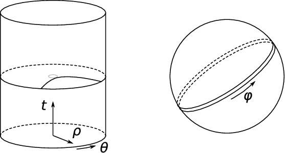
We sketch the profile of one arc (two joined half-arcs each described by the above asymptotic solution) of the string located in $AdS_{3}$ which also circles $S^{1}$ in Figure 1.

Refer to caption — Figure 1: Profile of an arc of fast-spinning string in $AdS_{3}$ wound around a big circle of $S^{5}$ .

One may of course construct a closed string solution out of 4 half-arcs each described by (3.43) by considering one arc in Figure 1 folded on itself. In this case $n$ will be equal to 2 and the energy (3.48) will have a smooth limit $m\to 0$ matching the energy of the straight folded string non-winding case. It is not clear, however, if such asymptotic closed string solution can be considered as a large spin limit of a finite spin closed string solution (see also sect. 3 of [27] for similar remarks). If the latter exists, it should probably be described by a more general ansatz than (3.32); also, in that case there would be, in contrast to what happens in the straight folded string case, a discontinuity between the small spin limit (described by an approximately elliptic string) and the large spin limit (described by that bent folded string).

As was already mentioned, the above asymptotic solution (3.43) should be equivalent to a particular asymptotic limit of the “rounded” spiky string solution with rotation and winding in a big circle of $S^{5}$ considered in [25]. Indeed, the large spin limit of the spiky string is conformally equivalent to the large spin limit of the straight string [26] and the same should be true for $\nu m\not=0$ .

Let us also note that a background similar to (3.43) appeared in [27] as a large spin limit of the $S_{1}=S_{2}$ solution in $AdS_{5}$ [27, 28]. Its interpretation, however, was different: there the angles of the $S^{3}\subset AdS_{5}$ ( $ds^{2}=d\theta^{2}+\cos^{2}\theta\ d\phi_{1}^{2}+\sin^{2}\theta\ d\phi_{1}^{2}$ ) were $\theta=\vartheta(\sigma),\ \phi_{1}=\phi_{2}=\kappa\tau$ , while here $\theta=\kappa\tau+\vartheta(\sigma),\ \phi_{1}=\phi_{2}=0$ . The asymptotic large spin solution in [27] was shown there to be $SO(2,4)$ equivalent to the asymptotic limit of the folded spinning string. This is no longer so for the present solution (3.43) as we shall discuss below.

3.4 Equivalence between the generalized null cusp and the large spin limit of the closed string solution

Writing the solution (3.43) in the embedding $AdS_{5}$ coordinates

\displaystyle X_{0}+\mathrm{i}X_{5}=\cosh\rho\ e^{\mathrm{i}t},\ \ \ \ \ \ \ \ X_{1}+\mathrm{i}X_{2}=\sinh\rho\ e^{\mathrm{i}\theta},\ \ \ \ \ \ X_{3}=X_{4}=0

(3.50)

we get

\displaystyle X_{0}+\mathrm{i}X_{5}

\displaystyle=\sqrt{1+\gamma^{2}}\ \cosh(\mu\sigma)\ e^{\mathrm{i}\kappa\tau}\ ,\ \ \ \ \ \ \ \ \ X_{1}+\mathrm{i}X_{2}

\displaystyle=\big[\sinh(\mu\sigma)+\mathrm{i}\gamma\cosh(\mu\sigma)\big]\ e^{\mathrm{i}\kappa\tau}\ ,

(3.51)

implying that

X_{0}X_{2}-X_{1}X_{5}={\textstyle{\gamma\over{\sqrt{1+\gamma^{2}}}}}(X_{0}^{2}+X_{5}^{2})\ ,\ \qquad\ \ X_{0}^{2}+X_{5}^{2}-X_{1}^{2}-X_{2}^{2}=1\ .

(3.52)

By applying two $SO(2,2)$ boosts in the planes $(02)$ and $(15)$

	$\displaystyle X_{0}=\cosh vY_{0}+\sinh vY_{2},\ \ \ \ \ \ \ X_{2}=\hphantom{-}\sinh vY_{0}+\cosh vY_{2},$		(3.53)
	$\displaystyle X_{1}=\cosh vY_{1}-\sinh vY_{5},\ \ \ \ \ \ \ X_{5}=-\sinh vY_{1}+\cosh vY_{5}\ ,\ \ \ \ \ \tanh(2v)={\textstyle{\gamma\over{\sqrt{1+\gamma^{2}}}}}$		(3.54)

we can transform the equation for world surface (3.52) into the form

Y_{0}Y_{2}-Y_{1}Y_{5}={\textstyle{1\over 2}}\gamma\ ,\qquad\ \ \ \ Y_{0}^{2}+Y_{5}^{2}-Y_{1}^{2}-Y_{2}^{2}=1\ .

(3.55)

Comparing this to (3.27) we observe that the euclidean world sheet solution for the null cusp is related to the Minkowski world sheet solution for the asymptotic limit of the closed string by the following analytic continuation¹⁸¹⁸ 18 The continuation of $Y_{2},Y_{5}$ is induced by continuation of the time-like world sheet coordinate.

	$\displaystyle Y_{0}\to Y_{0},\qquad Y_{1}\to Y_{1},\quad Y_{2}\to\mathrm{i}Y_{2},\quad Y_{5}\to\mathrm{i}Y_{5},$		(3.56)
	$\displaystyle\nu_{{}_{e}}\to\mathrm{i}\nu,\ \ \ \mu\to\mu,\ \ \ \kappa\to\kappa,\ \ \ m\to m,\ \ \gamma_{{}_{e}}\to\mathrm{i}\gamma,\ \quad{\textstyle{1\over 2}}\hat{\kappa}t\to-\mathrm{i}\kappa\tau,\ \ \ {\textstyle{1\over 2}}s\to\mu\sigma$		(3.57)

Here the transformations of the world sheet coordinates can be found, e.g. by comparing the expressions for the $S^{5}$ angle $\varphi$ in (3.20) and in (1.14), (3.32) ( $\varphi$ remains real under the euclidean rotation, with $\nu$ and $\tau$ rotating in “opposite” directions).

Following the same logic as in [11] (where the null cusp with $\nu=0$ was considered) and in [12] (where the $\nu\not=0$ generalization was considered) below we shall use the euclidean null cusp form of the solution (3.16) or (3.20) to compute the string partition function $Z(\hat{\nu},\hat{m})$ in the 2-loop approximation, defining it in terms of the path integral with the string action (3.7) in the AdS light-cone gauge. We shall then extract from $W=-\ln Z$ the expression for the generalized scaling function by applying the relations (2.13)–(2.22) from section 2.

As we are ultimately interested in the dependence on the parameters of the closed-string solution (1.14), (1.15), we shall rotate the parameters of the open string solution (3.16), (3.20) as in (3.57), i.e. $\nu\to\mathrm{i}\nu$ . It turns out to be useful to keep a symmetry between $\nu$ and $m$ , so we shall use the solution (3.16), (3.20) with the imaginary $\nu_{{}_{e}}=\mathrm{i}\nu$ and the imaginary $m\equiv\mathrm{i}w$ (thus keeping $\nu_{{}_{e}}m=-\nu w$ in $x^{-}$ in (3.20) real), i.e. we shall start with (cf. (3.22))

	$\displaystyle\varphi={\textstyle{1\over 2}}\mathrm{i}(\hat{\nu}t+\hat{w}s)\ ,\ \ \ \ \ \ \ \ \ \hat{w}\equiv-\mathrm{i}\hat{m}\ ,\ \ \ \ \ \ \ \ \hat{\kappa}=\sqrt{1+\hat{\nu}^{2}-\hat{w}^{2}}\ ,$		(3.58)
	$\displaystyle I_{E}=\frac{\sqrt{\lambda}}{2\pi}(1-\hat{w}^{2})V\ .$		(3.59)

We should of course set $w=-\mathrm{i}m$ , i.e. replace $w$ by the physical closed-string winding number $m$ in (1.14) in the final expression for the partition function.

The remarkable property of the generalized null cusp solution (3.16), (3.20) or the equivalent Minkowski world sheet solution (1.14), (1.15), (3.43) is that, as in the zero-winding $m=0$ case [18], it is still a homogeneous solution, i.e. it can be put into the form where only the isometric angles of the $AdS_{5}$ metric are non-zero and linear in $(\tau,\sigma)$ . In this case the fluctuation Lagrangian can be put into a form where it will have constant ( $(\tau,\sigma)$ -independent) coefficients and thus the computation of quantum corrections can be done by standard diagrammatic methods. Starting with the form of the solution in (3.25) the argument is essentially the same as in [18]. Namely, let us introduce the new global $AdS_{5}$ coordinates $(\beta,r,p,q,h)$ by setting

	$\displaystyle X_{0}\pm X_{3}=\ \cosh r\ \sin\beta\ e^{\pm p},\ \ \ X_{5}\pm X_{4}=\ \cosh r\ \cos\beta\ e^{\pm q}\ ,\ \ \ X_{1}\pm{\rm i}X_{2}=\ \sinh r\ e^{\pm{\rm i}h}$
	$\displaystyle ds^{2}=-\cosh^{2}r\ d\beta^{2}+dr^{2}+\cosh^{2}r\ (\sin^{2}\beta\ dp^{2}+\cos^{2}\beta\ dq^{2})+\sinh^{2}r\ dh^{2}$		(3.60)

As follows from (3.20), (3.21), (3.25), in the case of the generalized null cusp

\displaystyle\cos(2\beta)=\gamma_{{}_{e}}\ ,\ \ \ \ p={\textstyle{1\over 2}}(\hat{\kappa}t+s)\ ,\ \ \ q={\textstyle{1\over 2}}(\hat{\kappa}t-s)\ ,\ \ \ \ \ \ \ r=0\ ,\ \ \ \ h=0\ .

(3.61)

It is easy to check that conformal-gauge conditions are satisfied if this background is supplemented by $\varphi={\textstyle{1\over 2}}(\hat{\nu}_{{}_{e}}t+\hat{m}s)$ in (3.20). Since only the isometric directions $p$ and $q$ are non-constant and are only linear in world-sheet coordinates this is a homogeneous background.

4 Expansion of the string action near the classical solution
and the 1-loop partition function

Let us now expand the euclidean light-cone gauge Lagrangian (3.7) near the classical solution (3.16) or (3.20), with $\nu_{{}_{e}}=\mathrm{i}\nu,\ m=\mathrm{i}w$ as in (3.58), and explicitly identify a field redefinition that puts the fluctuation Lagrangian into the form where it has constant coefficients. This will enable us to compute the corresponding partition function in semiclassical expansion by evaluating standard Feynman diagrams. The 1-loop partition function will be determined by the quadratic part of the fluctuation action. The 2-loop corrections will be discussed in the next section.

4.1 Expansion of the action

It is useful to construct the expansion of the action two steps: we shall first consider only the expansion near $z$ background in (3.16) and will include the $\varphi$ background in (3.58) later.

The first step is essentially identical to the expansion of the action around the standard ( $\nu,w=0$ ) null cusp solution [23]. It is useful to define the fluctuations around the $z$ solution with extra rescalings

	$\displaystyle z=\sqrt{{\hat{\kappa}}}\,\sqrt{\frac{\tau}{\sigma}}\ {\tilde{z}}~,~~~z^{M}=\sqrt{{\hat{\kappa}}}\,\sqrt{\frac{\tau}{\sigma}}\ {\tilde{z}}^{M}~\ ,\ \ \ \ x=\sqrt{{\hat{\kappa}}}\,\sqrt{\frac{\tau}{\sigma}}{\tilde{x}}~,~~~~\theta=\frac{1}{\sqrt{\sigma}}{\tilde{\theta}}~,~~~~\eta=\frac{1}{\sqrt{\sigma}}{\tilde{\eta}}\ ,$		(4.1)
	$\displaystyle{\tilde{x}}={\tilde{x}}_{1}+{\rm i}{\tilde{x}}_{2}\ ,\ \ \ \ ~~~~{\tilde{z}}\equiv e^{\tilde{\phi}}=1+\tilde{\phi}+...\ ,\ \ \ \ ~~~~{\tilde{z}}^{M}={\tilde{z}}u^{M}\ ,\ \ \ \ ~~~~u^{M}u^{M}=1~~.$		(4.2)

Then the Lagrangian written in terms of the coordinates $(s,t)$ in (3.18) becomes (we rescale overall factor of $\hat{\kappa}^{2}$ )

$\displaystyle{\cal L}$	$\displaystyle=$	$\displaystyle\big\|\partial_{t}{\tilde{x}}+\frac{1}{2}{\hat{\kappa}}\,{\tilde{x}}\big\|^{2}+(\partial_{t}{\tilde{z}}^{M}+\frac{1}{2}{\hat{\kappa}}\,{\tilde{z}}^{M}+\frac{{\rm i}}{{\tilde{z}}^{2}}{\tilde{\eta}}_{i}\rho^{MN}{}^{i}{}_{j}{\tilde{\eta}}^{j}{\tilde{z}}^{N})^{2}$	(4.6)
		$\displaystyle~~~~~~~~~~~~~~~~~~~~~~+\ \frac{1}{{\tilde{z}}^{4}}\Big[\big\|\partial_{s}{\tilde{x}}-\frac{1}{2}{\tilde{x}}\big\|^{2}+(\partial_{s}{\tilde{z}}^{M}-\frac{1}{2}{\tilde{z}}^{M})^{2}\Big]$
		$\displaystyle~~~~~~~~~~~~~~~~~~~~~+{\rm i}({\tilde{\theta}}^{i}\partial_{t}{\tilde{\theta}}_{i}+{\tilde{\eta}}^{i}\partial_{t}{\tilde{\eta}}_{i}+{\tilde{\theta}}_{i}\partial_{t}{\tilde{\theta}}^{i}+{\tilde{\eta}}_{i}\partial_{t}{\tilde{\eta}}^{i})-\ \frac{1}{{\tilde{z}}^{2}}({\tilde{\eta}}^{2})^{2}$
		$\displaystyle+2\ {\rm i}\Bigl[\ \frac{1}{{\tilde{z}}^{3}}{\tilde{\eta}}^{i}\rho_{ij}^{M}{\tilde{z}}^{M}(\partial_{s}{\tilde{\theta}}^{j}-\frac{1}{2}{\tilde{\theta}}^{j}-\frac{1}{{\tilde{z}}}{\tilde{\eta}}^{j}(\partial_{s}{\tilde{x}}-\frac{1}{2}{\tilde{x}}))$
		$\displaystyle~~~~~~~~~~~~~~~~~~~~~+\frac{1}{{\tilde{z}}^{3}}{\tilde{\eta}}_{i}(\rho^{\dagger}_{M})^{ij}{\tilde{z}}^{M}\big(\partial_{s}{\tilde{\theta}}_{j}-\frac{1}{2}{\tilde{\theta}}_{j}+\frac{{\rm i}}{{\tilde{z}}}{\tilde{\eta}}_{j}(\partial_{s}{\tilde{x}}^{}-\frac{1}{2}{\tilde{x}}^{})\big)\Bigr]\ .$	(4.7)

Let us now discuss the dependence on the $S^{5}$ angle $\varphi$ in (3.3). Since $\varphi$ represents an isometry direction, it should be possible to find a coordinate transformation such that only the derivatives of $\varphi$ appear in the action. According to (3.3) the angle $\varphi$ may be shifted by a rotation in the $(56)$ plane. Let us make such a rotation with an arbitrary angle $\check{\varphi}$ , (the rotation matrix $R(\check{\varphi})$ acts in $(56)$ plane)

(R\tilde{z})^{A}=R^{A}_{\hphantom{A}B}\tilde{z}^{B}\ ,\ \ \ \ \ \ \ \ R=\begin{pmatrix}\hphantom{-}\cos\check{\varphi}&\sin\check{\varphi}\\ -\sin\check{\varphi}&\cos\check{\varphi}\end{pmatrix}\ ,\ \ \ \ \ \ (\partial R)R^{-1}=\partial{\check{\varphi}}\begin{pmatrix}0&1\cr-1&0\end{pmatrix}~~.

(4.8)

To define the action of this rotation on the fermions, let us introduce the following matrices

	$\displaystyle M^{i}_{\hphantom{i}j}(\check{\varphi})$	$\displaystyle=\exp(-\frac{1}{2}\rho^{\dagger[5}\rho^{6]}\check{\varphi})^{i}_{\hphantom{i}j}=\delta_{j}^{i}\cos\frac{\check{\varphi}}{2}-(\rho^{\dagger[5}\rho^{6]})^{i}_{\hphantom{i}j}\ \sin\frac{\check{\varphi}}{2},$		(4.9)
	$\displaystyle M_{i}^{\hphantom{i}j}(\check{\varphi})$	$\displaystyle=\exp(-\frac{1}{2}\rho^{[5}\rho^{\dagger 6]}\check{\varphi})_{i}^{\hphantom{i}j}=\delta_{i}^{j}\cos\frac{\check{\varphi}}{2}-(\rho^{[5}\rho^{\dagger 6]})_{i}^{\hphantom{i}j}\ \sin\frac{\check{\varphi}}{2}.$		(4.10)

Then the action of the rotation $R$ on the fermions $\theta$ is (the action on $\eta$ is the same)

\displaystyle\theta^{i}\to M^{i}_{\hphantom{i}j}(\check{\varphi})\theta^{j}=\theta^{j}M_{j}^{\hphantom{j}i}(-\check{\varphi}),\ \ \ \ \ \ \ \ \ \theta_{i}\to M_{i}^{\hphantom{i}j}(\check{\varphi})\theta_{j}=\theta_{j}M^{j}_{\hphantom{j}i}(-\check{\varphi}).

(4.11)

In the representation we are using the matrices $\rho^{\dagger[5}\rho^{6]}$ and $\rho^{[5}\rho^{\dagger 6]}$ are diagonal, purely imaginary and complex conjugate of each other. If $\check{\varphi}$ were a constant, this would be a symmetry of the action. We may then use such rotation to eliminate the dependence of the action on the constant part of $\varphi$ , i.e. to make the action depend only on derivatives of $\varphi$ ; in this case the action will have constant coefficients since $\varphi$ in (3.58) is linear function of the world sheet coordinates. The rotated form of the action can be written as

$\displaystyle{\cal L}$	$\displaystyle=$	$\displaystyle~~\big\|\partial_{t}{\tilde{x}}+\frac{1}{2}{\hat{\kappa}}\,{\tilde{x}}\big\|^{2}$	(4.16)
		$\displaystyle+\Big(\partial_{t}(R{\tilde{z}})^{M}-[((\partial_{t}R)R^{-1})(R{\tilde{z}})]^{M}+\frac{1}{2}{\hat{\kappa}}\,(R{\tilde{z}})^{M}+\frac{{\rm i}}{{\tilde{z}}^{2}}{{\tilde{\eta}}}_{i}\rho^{MN}{}^{i}{}_{j}{{\tilde{\eta}}}^{j}(R{\tilde{z}})^{N}\Big)^{2}$
		$\displaystyle+\ \frac{1}{{\tilde{z}}^{4}}\Big[\big\|\partial_{s}{\tilde{x}}-\frac{1}{2}{\tilde{x}}\big\|^{2}+\Big(\partial_{s}R{\tilde{z}}^{M}-[((\partial_{s}R)R^{-1})(R{\tilde{z}})]^{M}-\frac{1}{2}R{\tilde{z}}^{M}\Big)^{2}\Big]$
		$\displaystyle~~~~~~~~~~~+{\rm i}\Big(\,{\tilde{\theta}}^{k}(\partial_{t}\delta^{k}_{l}-\frac{1}{2}\partial_{t}{\check{\varphi}}(\rho^{[5}\rho^{\dagger 6]}){}_{k}{}^{l}){\tilde{\theta}}_{l}+{\tilde{\eta}}^{k}(\partial_{t}\delta^{k}_{l}-\frac{1}{2}\partial_{t}{\check{\varphi}}(\rho^{[5}\rho^{\dagger 6]}){}_{k}{}^{l}){\tilde{\eta}}_{l}$
		$\displaystyle~~~~~~~~~~~~~~~+{\tilde{\theta}}_{k}(\partial_{t}\delta^{k}_{l}-\frac{1}{2}\partial_{t}{\check{\varphi}}(\rho^{\dagger[5}\rho^{6]}){}^{k}{}_{l}){\tilde{\theta}}^{l}+{\tilde{\eta}}_{k}(\partial_{t}\delta^{k}_{l}-\frac{1}{2}\partial_{t}{\check{\varphi}}(\rho^{\dagger[5}\rho^{6]}){}^{k}{}_{l}){\tilde{\eta}}^{l}\Big)-\ \frac{1}{{\tilde{z}}^{2}}({{\tilde{\eta}}}^{2})^{2}\bigg]$
		$\displaystyle+\ \frac{2{\rm i}}{{\tilde{z}}^{3}}\ \Bigl[\ {{\tilde{\eta}}}^{k}\rho_{kl}^{M}(R{\tilde{z}})^{M}\Big(\partial_{s}{{\tilde{\theta}}}^{l}-\frac{1}{2}\partial_{s}{\check{\varphi}}(\rho^{\dagger[5}\rho^{6]}){}^{l}{}_{u}{\tilde{\theta}}^{u}-\frac{1}{2}{{\tilde{\theta}}}^{l}-\frac{{\rm i}}{{\tilde{z}}}\,{{\tilde{\eta}}}^{l}(\partial_{s}{\tilde{x}}-\frac{1}{2}{\tilde{x}})\Big)$
		$\displaystyle~~~~~+{{\tilde{\eta}}}_{k}(\rho^{\dagger}_{M})^{kl}(R{\tilde{z}})^{M}\Big(\partial_{s}{{\tilde{\theta}}}_{l}-\frac{1}{2}\partial_{s}{\check{\varphi}}(\rho^{[5}\rho^{\dagger 6]}){}_{l}{}^{u}{\tilde{\theta}}_{u}-\frac{1}{2}{{\tilde{\theta}}}_{l}+\frac{{\rm i}}{{\tilde{z}}}\,{{\tilde{\eta}}}_{l}(\partial_{s}{\tilde{x}}^{}-\frac{1}{2}{\tilde{x}}^{})\Big)\Bigr]\ .$	(4.17)

Here bosonic connection term $(\partial_{t}R)R^{-1}$ vanishes in the directions $1,2,3,4$ ; in the $(56)$ plane it is given by (4.8).

A family of choices for the rotation angle ${\check{\varphi}}$ in $R$ which renders all coefficients in the action constant is

\check{\varphi}=\frac{\rm i}{2}(\hat{\nu}\,t+\hat{w}\,s)+\delta\,\tilde{\varphi}(t,s)\ ,

(4.18)

where the first term represents our classical background (3.58) and $\tilde{\varphi}(t,s)$ is the fluctuation field. The parameter $\delta$ may be further changed arbitrarily by background-independent rotations. It should disappear from all $SO(6)$ -invariant quantities; we shall keep it at intermediate stages as this provides a test of the calculations.¹⁹¹⁹ 19 The bosonic part of the Lagrangian is actually independent of $\delta$ , but interaction terms involving fermions have a non-trivial dependence on it. Also, for $\delta\neq 1$ , the action contains terms with no derivatives on ${\tilde{\varphi}}$ . Using (3.3) the rotated coordinates are then ( $a=1,\ldots,4$ )

\displaystyle(R\tilde{z})^{a}=e^{\tilde{\phi}}\,\frac{y^{a}}{1+{\textstyle\frac{1}{4}}y^{2}}\,,~~~~\ \ \ \ \ \ (R\tilde{z})^{5}+{\rm i}(R\tilde{z})^{6}=e^{\tilde{\phi}}\,\frac{1-{\textstyle\frac{1}{4}}y^{2}}{1+{\textstyle{\textstyle{\textstyle\frac{1}{4}}}}y^{2}}\,\ e^{{\rm i}(1-\delta)\tilde{\varphi}}

(4.19)

4.2 Quadratic part of the action

It is easy to extract the quadratic bosonic part of (4.17) (we ignore total derivatives and also drop a term linear in fluctuations and proportional to $(1+{\hat{\nu}}^{2}-{\hat{w}}^{2}-\hat{\kappa}^{2})$ ; here $\alpha=(t,s)$ )

$\displaystyle{\cal L}_{B}^{(2)}$	$\displaystyle=\partial_{\alpha}\tilde{x}\partial_{\alpha}\tilde{x}^{}+{\textstyle{\textstyle\frac{1}{4}}}(1+\hat{\kappa}^{2})\tilde{x}\tilde{x}^{}+\partial_{\alpha}y^{a}\partial_{\alpha}y^{a}+{\textstyle{\textstyle\frac{1}{4}}}(\hat{\nu}^{2}+\hat{w}^{2})y^{a}y^{a}$	(4.20)
	$\displaystyle+\partial_{\alpha}\tilde{\phi}\partial_{\alpha}\tilde{\phi}+\partial_{\alpha}\tilde{\varphi}\partial_{\alpha}\tilde{\varphi}+2{\rm i}(\hat{\nu}\partial_{t}\tilde{\varphi}-\hat{w}\partial_{s}\tilde{\varphi})\tilde{\phi}+(\hat{\kappa}^{2}-\hat{\nu}^{2})\tilde{\phi}^{2}$
	$\displaystyle\equiv({\tilde{x}},{\tilde{x}}^{},{\tilde{\phi}},{\tilde{\varphi}},{y}_{a})K_{B}({\tilde{x}},{\tilde{x}}^{},{\tilde{\phi}},{\tilde{\varphi}},{y}_{a})^{T}~~.$

The bosonic propagator is then (note the overall factor of $1/2$ in the action (3.5))

	$\displaystyle G_{B}(p)\equiv K_{B}^{-1}(p)$	$\displaystyle=$	$\displaystyle\begin{pmatrix}0&\frac{2}{p^{2}+{\textstyle{\textstyle\frac{1}{4}}}(1+{\hat{\kappa}}^{2})}&0&0&{\bf 0}_{1\times 4}\cr\frac{2}{p^{2}+{\textstyle{\textstyle\frac{1}{4}}}(1+{\hat{\kappa}}^{2})}&0&0&0&{\bf 0}_{1\times 4}\cr 0&0&\frac{p^{2}}{{\cal D}_{B}(p)}&\frac{{\hat{\nu}}p_{0}-{\hat{w}}p_{1}}{{\cal D}_{B}(p)}&{\bf 0}_{1\times 4}\cr 0&0&\frac{-{{\hat{\nu}}}p_{0}+{\hat{w}}p_{1}}{{\cal D}_{B}(p)}&\frac{{\hat{\kappa}}^{2}-{\hat{\nu}}^{2}+p^{2}}{{\cal D}_{B}(p)}&{\bf 0}_{1\times 4}\cr{\bf 0}_{4\times 1}&{\bf 0}_{4\times 1}&{\bf 0}_{4\times 1}&{\bf 0}_{4\times 1}&\frac{{\bf 1}_{4\times 4}}{p^{2}+{\textstyle{\textstyle\frac{1}{4}}}({\hat{\nu}}^{2}+{\hat{w}}^{2})}\end{pmatrix}$		(4.21)
	$\displaystyle{\cal D}_{B}(p)$	$\displaystyle\equiv$	$\displaystyle p^{4}+\hat{\kappa}^{2}p_{0}^{2}+p_{1}^{2}-2\hat{\nu}\hat{w}\,p_{0}p_{1}=p^{2}(p^{2}+1)+(\hat{\nu}^{2}-\hat{w}^{2})p_{0}^{2}-2\hat{\nu}\hat{w}\,p_{0}p_{1}\ .$		(4.22)

One may easily identify the bosonic fluctuation spectrum from the poles of this propagator: it consists of eight massive fields and for ${\hat{w}}=0$ reproduces the massive part of the conformal gauge bosonic fluctuation spectrum [5] around the solution (1.3). The terms quadratic in fermions extracted from (4.17) are:

$\displaystyle{\cal L}_{F}^{(2)}=$	$\displaystyle\rm{\displaystyle i}\Bigr[\,{\tilde{\theta}}^{k}(\partial_{t}\delta^{k}_{l}-\frac{\mathrm{i}\hat{\nu}}{4}(\rho^{[5}\rho^{\dagger 6]}){}_{k}{}^{l}){\tilde{\theta}}_{l}+{\tilde{\eta}}^{k}(\partial_{t}\delta^{k}_{l}-\frac{3\mathrm{i}\hat{\nu}}{4}(\rho^{[5}\rho^{\dagger 6]}){}_{k}{}^{l}){\tilde{\eta}}_{l}$	(4.23)
	$\displaystyle+{\tilde{\theta}}_{k}(\partial_{t}\delta^{k}_{l}-\frac{\mathrm{i}\hat{\nu}}{4}(\rho^{\dagger[5}\rho^{6]}){}^{k}{}_{l}){\tilde{\theta}}^{l}+{\tilde{\eta}}_{k}(\partial_{t}\delta^{k}_{l}-\frac{3\mathrm{i}\hat{\nu}}{4}(\rho^{\dagger[5}\rho^{6]}){}^{k}{}_{l}){\tilde{\eta}}^{l}\Bigr]$
	$\displaystyle+2{\rm i}\Bigl[{{\tilde{\eta}}}^{k}\rho_{kl}^{5}\Big(\partial_{s}{{\tilde{\theta}}}^{l}-\frac{\mathrm{i}\hat{w}}{4}(\rho^{\dagger[5}\rho^{6]}){}^{l}{}_{u}{\tilde{\theta}}^{u}-\frac{1}{2}{{\tilde{\theta}}}^{l}\Big)+{{\tilde{\eta}}}_{k}(\rho^{\dagger}_{5})^{kl}\Big(\partial_{s}{{\tilde{\theta}}}_{l}-\frac{\mathrm{i}\hat{w}}{4}(\rho^{[5}\rho^{\dagger 6]}){}_{l}{}^{u}{\tilde{\theta}}_{u}-\frac{1}{2}{{\tilde{\theta}}}_{l}\Big)\Bigr]$
$\displaystyle\equiv$	$\displaystyle(\tilde{\theta}^{i},\tilde{\theta}_{i},\tilde{\eta}^{i},\tilde{\eta}_{i})K_{F}(\tilde{\theta}^{i},\tilde{\theta}_{i},\tilde{\eta}^{i},\tilde{\eta}_{i})^{T}~~.$

The corresponding kinetic operator matrix in the momentum space is

K_{F}={\rm i}\begin{pmatrix}0&{\rm i}p_{0}{\bf 1}_{4}-\frac{{\rm i}\hat{\nu}}{4}\rho^{[5}\rho^{\dagger\,6]}&-({\rm i}p_{1}+\textstyle{\frac{1}{2}})\rho^{5}-\frac{{\rm i}\hat{w}}{4}\rho^{6}&0\cr{\rm i}p_{0}{\bf 1}_{4}-\frac{{\rm i}\hat{\nu}}{4}\rho^{\dagger[5}\rho^{6]}&0&0&-({\rm i}p_{1}+\textstyle{\frac{1}{2}})\rho^{\dagger}_{5}-\frac{{\rm i}\hat{w}}{4}\rho^{\dagger}_{6}\cr({\rm i}p_{1}-\textstyle{\frac{1}{2}})\rho^{5}-\frac{{\rm i}\hat{w}}{4}\rho^{6}&0&0&{\rm i}p_{0}{\bf 1}_{4}-\frac{3{\rm i}\hat{\nu}}{4}\rho^{[5}\rho^{\dagger\,6]}\cr 0&({\rm i}p_{1}-\textstyle{\frac{1}{2}})\rho^{\dagger}_{5}-\frac{{\rm i}\hat{w}}{4}\rho^{\dagger}_{6}&{\rm i}p_{0}{\bf 1}_{4}-\frac{3{\rm i}\hat{\nu}}{4}\rho^{\dagger[5}\rho^{6]}&0\end{pmatrix}~~.

(4.24)

Its inverse is somewhat complicated so we present it in Appendix E. It has the following structure, which exposes its poles

\displaystyle K_{F}^{-1}(p)=\frac{N_{+}(p)}{{\cal D}_{F}(p)}+\frac{N_{-}(p)}{{\cal D}_{F}^{*}(p)}~,\ ~~~~~\ \ \ {\cal D}_{F}(p)=(p_{0}-\frac{{\rm i}{\hat{\nu}}}{4})^{2}+(p_{1}+\frac{{\rm i}{\hat{w}}}{4})^{2}+\frac{{{\hat{\kappa}}}^{2}+{{\hat{w}}}^{2}}{4}\ .

(4.25)

All 8 fermions are thus massive with equal masses. This is consistent with the surviving $SO(4)$ symmetry and charge conjugation [8].

4.3 One-loop partition function

Using the determinants of the kinetic operators (4.21) and (4.24)

	$\displaystyle\det K_{B}$	$\displaystyle=$	$\displaystyle\big[p^{2}+{\textstyle{\textstyle\frac{1}{4}}}(1+\hat{\kappa}^{2})\big]^{2}\left(p^{4}+\hat{\kappa}^{2}p_{0}^{2}+p_{1}^{2}-2\hat{\nu}\hat{w}\,p_{0}p_{1}\right)\big[p^{2}+{\textstyle{\textstyle\frac{1}{4}}}(\hat{\nu}^{2}+\hat{w}^{2})\big]^{4}$		(4.26)
	$\displaystyle\det K_{F}$	$\displaystyle=$	$\displaystyle\Big[\big(p^{2}+\frac{4\hat{\kappa}^{2}-\hat{\nu}^{2}+3\hat{w}^{2}}{16}\big)^{2}+{\textstyle{\textstyle\frac{1}{4}}}(\hat{\nu}p_{0}-\hat{w}p_{1})^{2}\Big]^{4}~~,$		(4.27)

one finds for the the one-loop contribution to the partition function in (1.19), (1.20)

\displaystyle Z_{1}=e^{-W_{1}}\ ,\ \ \ \ \ \ \ \ \ \ W_{1}=\frac{V}{2\pi}{\cal F}_{1}(\hat{\nu},\hat{w})\ ,\ \ \ \ \ \ V={1\over 4}\int dtds={1\over 4}V_{2}\ ,

(4.28)

	$\displaystyle{\cal F}_{1}=4\pi\int\frac{d^{2}p}{(2\pi)^{2}}\Bigr(2\ln\big[p^{2}+{\textstyle{\textstyle\frac{1}{4}}}(1+\hat{\kappa}^{2})\big]+\ln(p^{4}+\hat{\kappa}^{2}p_{0}^{2}+p_{1}^{2}-2\hat{\nu}\hat{w}\,p_{0}p_{1})+4\ln\big[p^{2}+{\textstyle{\textstyle\frac{1}{4}}}(\hat{\nu}^{2}+\hat{w}^{2})\big]$
	$\displaystyle~~~~~~~~~~~~~~~~~~-4\ln\big[\big(p^{2}+\frac{4\hat{\kappa}^{2}-\hat{\nu}^{2}+3\hat{w}^{2}}{16}\big)^{2}+{\textstyle{\textstyle\frac{1}{4}}}(\hat{\nu}p_{0}-\hat{w}p_{1})^{2}\big]\Bigr)~~.$		(4.29)

The constraint ${\hat{\kappa}}^{2}=1+{\hat{\nu}}^{2}-{\hat{w}}^{2}$ in the solution (3.58) then implies that the momentum integral converges in the UV.²⁰²⁰ 20 Note that there is an instability coming from $S^{5}$ fluctuations for small enough orbital momentum or large enough winding, $\hat{m}^{2}=-\hat{w}^{2}>\hat{\nu}^{2}$ . The same instability was present in the case of the circular $(S,J)$ string solution [33] (with ${\cal S}n+{\cal J}m=0$ ); it is of course absent in large ${\cal J}=\nu$ expansion for finite $m$ . Evaluating this integral leads to

	$\displaystyle{\cal F}_{1}(\hat{\nu},\hat{w})=$	$\displaystyle-1+\hat{w}^{2}+\sqrt{(1+\hat{\nu}^{2})(1-\hat{w}^{2})}-(\hat{\nu}^{2}+\hat{w}^{2})\ln(\hat{\nu}^{2}+\hat{w}^{2})+2(1+\hat{\nu}^{2})\ln(1+\hat{\nu}^{2})$		(4.30)
		$\displaystyle-(2+\hat{\nu}^{2}-\hat{w}^{2})\ln\big[\sqrt{2+\hat{\nu}^{2}-\hat{w}^{2}}(\sqrt{1+\hat{\nu}^{2}}+\sqrt{1-\hat{w}^{2}})\big]\ .$		(4.30)

For ${\hat{w}}=0$ we thus recover the result for the asymptotic $(S,J)$ folded string (1.3) or for the null cusp with $\nu\not=0$ obtained in conformal gauge in [5, 12]. Note that $W_{1}$ is invariant under the simultaneous exchanges $\nu\leftrightarrow w,~~\kappa\leftrightarrow\mu,~~V_{2}\leftrightarrow{\hat{\kappa}}^{2}V_{2}~,$ as implied by the symmetry of the classical solution (3.20), (3.58).

5 Two-loop partition function

In this section we shall present the calculation of the 2-loop term in the logarithm of the partition function in (1.19), (1.20), i.e.

W_{2}=\frac{V}{2\pi\sqrt{\lambda}}\,{\cal F}_{2}(\hat{\nu},\hat{w})\,.

(5.1)

$W_{2}$ receives contributions from all connected vacuum diagrams that have the one-particle irreducible (1PI) topologies in Fig.2 and the non-1PI “tadpole” topology in Fig.3. As in the case of the cusp without angular momentum on $S^{5}$ discussed in the AdS light-cone gauge in [23], here the non-1PI tadpole graphs are again non-vanishing and their contribution is important for the cancellation of 2-loop UV divergences and for reproducing the correct 2-loop term in the generalized scaling function which agrees with the Bethe ansatz result.

For the computation of the 2-loop Feynman diagrams we need to expand the action (4.17) to fourth order in the fluctuations

I=I^{(0)}+I^{(2)}+I_{int}^{(3)}+I_{int}^{(4)}+\ldots\ ,

(5.2)

where the structure of the interaction terms may be written schematically as

		$\displaystyle I_{int}^{(3)}=\frac{\sqrt{\lambda}}{2\pi}\int dtds\Big(\frac{1}{3!}V_{i_{B}j_{B}k_{B}}^{(B^{3})}\Phi^{i_{B}}\Phi^{j_{B}}\Phi^{k_{B}}+\frac{1}{2!}V_{i_{B}\|i_{F}j_{F}}^{(BF^{2})}\Phi^{i_{B}}\Psi^{i_{F}}\Psi^{j_{F}}\Big)$		(5.3)
		$\displaystyle I_{int}^{(4)}=\frac{\sqrt{\lambda}}{2\pi}\int dtds\Big(\frac{1}{4!}V_{i_{B}j_{B}k_{B}l_{B}}^{(B^{4})}\Phi^{i_{B}}\Phi^{j_{B}}\Phi^{k_{B}}\Phi^{l_{B}}+\frac{1}{(2!)^{2}}V_{i_{B}j_{B}\|i_{F}j_{F}}^{(B^{2}F^{2})}\Phi^{i_{B}}\Phi^{j_{B}}\Psi^{i_{F}}\Psi^{j_{F}}$
		$\displaystyle+\frac{1}{4!}V_{i_{F}j_{F}k_{F}l_{F}}^{(F^{4})}\Psi^{i_{F}}\Psi^{j_{F}}\Psi^{k_{F}}\Psi^{l_{F}}\Big)\,.$

Here $\Phi^{i_{B}}=(\tilde{\phi},\tilde{\varphi},\tilde{x},\tilde{x}^{*},y^{a})$ includes the 8 bosonic fluctuations and $\Psi^{i_{F}}=(\tilde{\theta}^{i},\tilde{\theta}_{i},\tilde{\eta}^{i},\tilde{\eta}_{i})$ the 16 fermionic ones. The vertices carry up to two derivatives or equivalently two momentum factors. The sunset and double-bubble contributions to $W=-\ln Z$ correspond to

\displaystyle W_{2~{\rm sunset}}=-\frac{1}{2}\langle I_{int}^{(3)}I_{int}^{(3)}\rangle_{{}_{\mbox{\scriptsize 1PI}}}\ ,\ \ \ \ \ \ \ \ \ \ \ \ \ \ W_{2~{\rm bubbles}}=\langle I_{int}^{(4)}\rangle\ ,

(5.4)

while the tadpole contribution is obtained from

W_{2~{\rm tadpoles}}=-\frac{1}{2}\langle I_{int}^{(3)}I_{int}^{(3)}\rangle_{{}_{\mbox{\scriptsize non-1PI}}}\,.

(5.5)

As usual, the expectation values above are to be computed by inserting the appropriate propagators derived from the quadratic part of the action (see (4.21), (4.24)).

In the following subsections we shall present some details of the computation of the relevant 2-loop Feynman diagrams. We begin with the analysis of the 1PI bosonic diagrams and later discuss the fermionic contributions. We end this section with the calculation of the tadpole contributions.

5.1 Bosonic Sunset

We can arrange the terms entering in the sunset diagram depending on their denominator structure. From the form of the interactions, we see that schematically we have the following possibilities

	$\displaystyle\int\frac{d^{2}p\,d^{2}q\,d^{2}r}{(2\pi)^{4}}\delta^{(2)}(p+q+r)\frac{{\cal N}(p,q,r)}{{\cal D}_{B}(p)(q^{2}+m^{2})(r^{2}+m^{2})}\,,~~~~m^{2}=m_{\tilde{x}}^{2}~{\rm or}~m_{y}^{2}$
	$\displaystyle\int\frac{d^{2}p\,d^{2}q\,d^{2}r}{(2\pi)^{4}}\delta^{(2)}(p+q+r)\frac{{\cal N}(p,q,r)}{{\cal D}_{B}(p){\cal D}_{B}(q){\cal D}_{B}(r)}\,,$		(5.6)

where the numerator ${\cal N}(p,q,r)$ contains tensors of up to fourth order in momenta, and ${\cal D}_{B}(p)$ is the denominator appearing in the $\tilde{\phi}$ and $\tilde{\varphi}$ propagators, see eq. (4.22). In (5.6) we have introduced the shorthand notation

\displaystyle m_{\tilde{x}}^{2}\equiv{\textstyle{\textstyle\frac{1}{4}}}(1+\hat{\kappa}^{2})\ ,\ \ \ \ \ \ \ \ \ \ m_{y}^{2}\equiv{\textstyle{\textstyle\frac{1}{4}}}(\hat{\nu}^{2}+\hat{w}^{2})

(5.7)

for the masses of the $\tilde{x}$ and $y^{a}$ fluctuations in (1.11), (4.21).

Unfortunately, the presence of the Lorentz non-invariant denominator ${\cal D}_{B}(p)$ (4.22) makes an exact evaluation of the loop integrals technically challenging. We will therefore limit ourselves to expanding up to fourth order in the parameters $\hat{\nu},\hat{w}$ . Since

\displaystyle\frac{1}{{\cal D}_{B}(p)}=\frac{1}{p^{2}(p^{2}+1)}+\frac{2\hat{\nu}\hat{w}p_{0}p_{1}+(\hat{w}^{2}-\hat{\nu}^{2})p_{0}^{2}}{p^{4}(p^{2}+1)^{2}}+\frac{[2\hat{\nu}\hat{w}p_{0}p_{1}+(\hat{w}^{2}-\hat{\nu}^{2})p_{0}^{2}]^{2}}{p^{6}(p^{2}+1)^{3}}+{\cal O}(\hat{\nu}^{6},\hat{w}^{6})\,,

(5.8)

we find that the denominators appearing in the expansion are Lorentz invariant, and therefore the evaluation of the loop integrals becomes straightforward.

For the computation of the sunset topology we need the third-order bosonic Lagrangian

	$\displaystyle{\cal L}_{B}^{(3)}=-4\,\tilde{\phi}\|\partial_{s}\tilde{x}-{\textstyle{1\over 2}}\tilde{x}\|^{2}+2\tilde{\phi}(\partial_{t}\tilde{\phi}^{2}-\partial_{s}\tilde{\phi}^{2})+2\tilde{\phi}(\partial_{t}\tilde{\varphi}^{2}-\partial_{s}\tilde{\varphi}^{2})+2{\rm i}\tilde{\phi}^{2}(\hat{\nu}\partial_{t}\tilde{\varphi}+\hat{w}\partial_{s}\tilde{\varphi})$
	$\displaystyle\ \ \ \ \ \ +\ \frac{1}{2}(\hat{\nu}^{2}-\hat{w}^{2})\,\tilde{\phi}\,y^{a}y^{a}+2\tilde{\phi}\left((\partial_{t}y^{a})^{2}-(\partial_{s}y^{a})^{2}\right)-{\rm i}(\hat{\nu}\partial_{t}\tilde{\varphi}+\hat{w}\partial_{s}\tilde{\varphi})\,y^{a}y^{a}\ .$		(5.9)

A particularly simple contribution, with a single ${\cal D}_{B}$ in the denominator, comes from the $\tilde{\phi}\tilde{x}\tilde{x}^{*}$ interaction. Evaluation of the corresponding Feynman diagram as obtained from (5.4) yields the integral²¹²¹ 21 Here and in the following we will omit the overall factor $\frac{2\pi}{\sqrt{\lambda}}V_{2}$ . It will be restored at the end.

-\frac{1}{2}\int\frac{d^{2}p\,d^{2}q\,d^{2}r}{(2\pi)^{4}}\,\delta^{(2)}(p+q+r)\frac{p^{2}(1+4\,q_{1}^{2})(1+4\,r_{1}^{2})}{{\cal D}_{B}(p)(q^{2}+m_{\tilde{x}}^{2})(r^{2}+m_{\tilde{x}}^{2})}\,.

(5.10)

After inserting the expansion in (5.8) we can perform the integral over the momenta by standard techniques, see Appendix B for more details. As in [11, 6], all manipulations of tensor structures in the numerators are performed in $d=2$ , and the resulting scalar integrals are evaluated using an analytic regularization scheme in which power divergent contribution are set to zero

\displaystyle\int\frac{d^{2}p}{(2\pi)^{2}}(p^{2})^{n}=0\,,\ \qquad n\,{\geqslant}\,0\,.

(5.11)

We also use the following notation for the integrals

	$\displaystyle{\rm I}\mbox{$\left({a\atop m^{2}}\right)$}$	$\displaystyle=$	$\displaystyle\int\frac{d^{2}p}{(2\pi)^{2}}\frac{1}{(p^{2}+m^{2})^{a}}\,,$
	$\displaystyle{\rm I}{\mbox{$\left({a_{1}\atop m_{1}^{2}}{a_{2}\atop m_{2}^{2}}{a_{3}\atop m_{3}^{2}}\right)$}}$	$\displaystyle=$	$\displaystyle\int\frac{d^{2}p\,d^{2}q\,d^{2}r}{(2\pi)^{4}}\,\frac{\delta^{(2)}(p+q+r)}{(p^{2}+m_{1}^{2})^{a_{1}}\,(q^{2}+m_{2}^{2})^{a_{2}}\,(r^{2}+m_{3}^{2})^{a_{3}}}\,.$		(5.12)

Note that the integrals ${\rm I}{\mbox{$\left({a_{1}\atop m_{1}^{2}}{a_{2}\atop m_{2}^{2}}{a_{3}\atop m_{3}^{2}}\right)$}}$ and ${\rm I}\mbox{$\left({a\atop m^{2}}\right)$}$ with $a>1$ are UV finite, while ${\rm I}\mbox{$\left({1\atop m^{2}}\right)$}$ is UV divergent. When any of the masses vanish, both types of integrals have IR divergences. In the following we will also use for convenience the notation ${\rm I}\mbox{$\left({1\atop m^{2}}\right)$}\equiv{\rm I}[m^{2}]$ . We refer to Appendices A, B and C for more details on evaluation of these integrals and their explicit values.

After reduction to scalar integrals and expansion up to fourth order in $\hat{\nu},\hat{w}$ , the integral (5.10) yields the following result

	$\displaystyle\!\!\!\!\!\!\!\!\!\!\hphantom{-}{\textstyle{\textstyle\frac{1}{4}}}{\rm I}{\mbox{$\left({1\atop 1}{1\atop{\textstyle{1\over 2}}}{1\atop{\textstyle{1\over 2}}}\right)$}}+{\textstyle{\textstyle\frac{1}{4}}}(\hat{\nu}^{2}-\hat{w}^{2})\left[{\rm I}{\mbox{$\left({1\atop 1}{1\atop{\textstyle{1\over 2}}}{1\atop{\textstyle{1\over 2}}}\right)$}}-\frac{1}{2}{\rm I}{\mbox{$\left({1\atop 1}{2\atop{\textstyle{1\over 2}}}{1\atop{\textstyle{1\over 2}}}\right)$}}-\frac{1}{2}{\rm I}{\mbox{$\left({2\atop 1}{1\atop{\textstyle{1\over 2}}}{1\atop{\textstyle{1\over 2}}}\right)$}}+4{\rm I}[1]{\rm I}[{\textstyle{1\over 2}}]\right]$		(5.13)
	$\displaystyle\!\!\!\!\!\!\!\!\!\!-\frac{1}{8}\Bigg[2\hat{\nu}^{2}\hat{w}^{2}{\rm I}{\mbox{$\left({1\atop 1}{1\atop{\textstyle{1\over 2}}}{1\atop{\textstyle{1\over 2}}}\right)$}}+(\hat{\nu}^{2}-\hat{w}^{2})^{2}\left({\rm I}{\mbox{$\left({2\atop 1}{1\atop{\textstyle{1\over 2}}}{1\atop{\textstyle{1\over 2}}}\right)$}}+{\rm I}{\mbox{$\left({1\atop 1}{2\atop{\textstyle{1\over 2}}}{1\atop{\textstyle{1\over 2}}}\right)$}}-{\textstyle{\textstyle\frac{1}{4}}}{\rm I}{\mbox{$\left({1\atop 1}{3\atop{\textstyle{1\over 2}}}{1\atop{\textstyle{1\over 2}}}\right)$}}-\frac{1}{2}{\rm I}{\mbox{$\left({2\atop 1}{2\atop{\textstyle{1\over 2}}}{1\atop{\textstyle{1\over 2}}}\right)$}}-\frac{1}{8}{\rm I}{\mbox{$\left({1\atop 1}{2\atop{\textstyle{1\over 2}}}{2\atop{\textstyle{1\over 2}}}\right)$}}\right)$		(5.14)
	$\displaystyle\;-\frac{1}{8}(5\hat{\nu}^{4}+2\hat{\nu}^{2}\hat{w}^{2}+5\hat{w}^{4}){\rm I}{\mbox{$\left({3\atop 1}{1\atop{\textstyle{1\over 2}}}{1\atop{\textstyle{1\over 2}}}\right)$}}+2(\hat{\nu}^{2}-\hat{w}^{2})^{2}{\rm I}[1]{\rm I}\mbox{$\left({2\atop{\textstyle{1\over 2}}}\right)$}+(3\hat{\nu}^{4}-10\hat{\nu}^{2}\hat{w}^{2}+3\hat{w}^{4}){\rm I}\mbox{$\left({2\atop 1}\right)$}{\rm I}[{\textstyle{1\over 2}}]\Bigg]$

The second contribution to the bosonic sunset with a single ${\cal D}_{B}(p)$ factor at the denominator comes from the cubic pieces in the Lagrangian which contain $y^{a}y^{a}$ while the cubic vertices involving the $\tilde{\phi}$ and $\tilde{\varphi}$ fluctuations have a denominator of the type ${\cal D}_{B}(p){\cal D}_{B}(q){\cal D}_{B}(r)$ . For brevity we do not present their expressions and give only the final result of the bosonic sunset. After expanding to fourth order in $\hat{\nu},\hat{w}$ and using the explicit values of the integrals from the Appendix C, we obtain

		$\displaystyle W_{2{\scriptstyle\rm B\ sunset}}=\frac{K}{16\pi^{2}}+\frac{1}{2}{\rm I}[1]^{2}+\frac{1}{32\pi^{2}}\Big[(\hat{\nu}^{2}-\hat{w}^{2})K+4\pi{\rm I}[1]\Big(\hat{\nu}^{2}(-1+2\ln 2+24\pi{\rm I}[1])$		(5.15)
		$\displaystyle+\hat{w}^{2}(1-2\ln 2+4\pi{\rm I}[1])\Big)+(\hat{\nu}^{2}+\hat{w}^{2})\ln m_{y}^{2}(\ln m_{y}^{2}-16\pi{\rm I}[1])\Big]$
		$\displaystyle-\frac{1}{1024\pi^{2}}\Big[\;\hat{\nu}^{4}(14K-9+24\ln 2+464\pi{\rm I}[1])+2\hat{\nu}^{2}\hat{w}^{2}(6K+19-40\ln 2-304\pi{\rm I}[1])$
		$\displaystyle+\hat{w}^{4}(14K-9+24\ln 2+80\pi{\rm I}[1])-32(\hat{\nu}^{4}-\hat{w}^{4})\ln m_{y}^{2}\Big]\,,$

where $K$ is the Catalan’s constant and $m_{y}^{2}={\textstyle{\textstyle\frac{1}{4}}}(\hat{\nu}^{2}+\hat{w}^{2})$ was defined in (5.7). To obtain the above expression we have rewritten all UV divergent 1-loop integrals in terms of ${\rm I}[1]$ , by using the identity ${\rm I}[m^{2}]={\rm I}[1]-\frac{1}{4\pi}\ln m^{2}$ , for $m^{2}\neq 0$ .

5.2 Bosonic double-bubble

Let us now give some details of the evaluation of the bosonic double-bubble diagram, which receives contributions from the bosonic quartic interactions

$\displaystyle{\cal L}^{(4)}_{B}\!\!$	$\displaystyle=$	$\displaystyle\!\!\frac{1}{3}(1-\hat{w}^{2})\tilde{\phi}^{4}+2\tilde{\phi}^{2}\partial_{\alpha}\tilde{\phi}\partial_{\alpha}\tilde{\phi}+\frac{4}{3}{\rm i}\,\tilde{\phi}^{3}(\hat{\nu}\partial_{t}\tilde{\phi}-\hat{w}\partial_{s}\tilde{\phi})-2{\rm i}\,\tilde{\phi}(\hat{\nu}\partial_{t}\tilde{\varphi}-\hat{w}\partial_{s}\tilde{\varphi})y^{a}y^{a}$	(5.16)
	$\displaystyle+$	$\displaystyle\!\!2\tilde{\phi}^{2}\partial_{\alpha}y^{a}\partial_{\alpha}y^{a}+{\textstyle{1\over 2}}\tilde{\phi}^{2}(\hat{\nu}^{2}+\hat{w}^{2})y^{2}+8\tilde{\phi}^{2}\|\partial_{s}\tilde{x}-{\textstyle{1\over 2}}\tilde{x}\|^{2}+2\tilde{\phi}^{2}\partial_{\alpha}\tilde{\varphi}\partial_{\alpha}\tilde{\varphi}-{\textstyle{1\over 2}}y^{2}\partial_{\alpha}y^{a}\partial_{\alpha}y^{a}$
	$\displaystyle-$	$\displaystyle\!\!\frac{1}{8}(\hat{\nu}^{2}+\hat{w}^{2})y^{4}-y^{a}y^{a}\partial_{\alpha}\tilde{\varphi}\partial_{\alpha}\tilde{\varphi}\,.$

From the form of the interactions, we see that the possible structures for the loop integrals are now

	$\displaystyle\int\frac{d^{2}p}{(2\pi)^{2}}\,\frac{d^{2}q}{(2\pi)^{2}}\frac{{\cal N}_{1}(p_{0},p_{1})}{p^{2}+m_{y}^{2}}\frac{{\cal N}_{2}(q_{0},q_{1})}{q^{2}+m_{y}^{2}}\,,$		(5.17)
	$\displaystyle\int\frac{d^{2}p}{(2\pi)^{2}}\,\frac{d^{2}q}{(2\pi)^{2}}\frac{{\cal N}_{1}(p_{0},p_{1})}{p^{2}+m^{2}}\frac{{\cal N}_{2}(q_{0},q_{1})}{{\cal D}_{B}(q)}\,,~~~~m^{2}=m_{\tilde{x}}^{2}~{\rm or}~m_{y}^{2}$		(5.18)
	$\displaystyle\int\frac{d^{2}p}{(2\pi)^{2}}\,\frac{d^{2}q}{(2\pi)^{2}}\frac{{\cal N}_{1}(p_{0},p_{1})}{{\cal D}_{B}(p)}\frac{{\cal N}_{2}(q_{0},q_{1})}{{\cal D}_{B}(q)}\,,$		(5.19)

where $p$ and $q$ are the momenta running in the two bubbles. The two loop integrals are independent and this makes it possible to evaluate them exactly despite the presence of the ${\cal D}_{B}(p)$ denominator. We can therefore compute the bosonic double-bubble graphs for any values of the $\hat{\nu},\hat{w}$ parameters. In view of combining the double-bubble contribution with the sunset diagram, we will however keep only terms up to fourth order in $\hat{\nu}$ and $\hat{w}$ in the final expression.

To systematically organize the calculation it is convenient to introduce the following notation

\displaystyle J_{B}(i,j)=\int\frac{d^{2}p}{(2\pi)^{2}}\frac{(p_{0})^{i}(p_{1})^{j}}{{\cal D}_{B}(p)}\,.

(5.20)

These integrals can be evaluated exactly, for example, by first computing the angular integral in the $(p_{0},p_{1})$ plane and then performing an integral over the modulus $|p|$ . In the process, one has to carefully separate a possible UV divergent part. The relevant explicit expressions for $J_{B}(i,j)$ are presented in Appendix A.

To give an example, let us present the contribution of the $x^{2}\tilde{\phi}^{2}$ -interaction in the Lagrangian which is of the type (5.18), namely,

\displaystyle\int\frac{d^{2}p\,d^{2}q}{(2\pi)^{4}}\frac{2p^{2}(1+4q_{1}^{2})}{{\cal D}_{B}(p)(q^{2}+m_{\tilde{x}}^{2})}=(\hat{w}^{2}-\hat{\nu}^{2})\big[J_{B}(0,2)+J_{B}(2,0)\big]\,{\rm I}[m_{\tilde{x}}^{2}]\,.

(5.21)

The other contributions can be computed analogously. After summing all the terms, using the explicit values of the integrals $J_{B}(i,j)$ and expanding up to fourth order in $\hat{\nu},\hat{w}$ , we obtain the following result for the bosonic double-bubble contribution

		$\displaystyle W_{2{\scriptstyle\rm B\ double-bubble}}=-{\textstyle{1\over 2}}{\rm I}[1]^{2}-\frac{1}{8\pi}{\rm I}[1]\left[\hat{\nu}^{2}(2\ln 2-1+24\pi\,{\rm I}[1])-\hat{w}^{2}(2\ln 2-1-4\pi\,{\rm I}[1])\right]$		(5.22)
		$\displaystyle-\frac{1}{32\pi^{2}}(\hat{\nu}^{2}+\hat{w}^{2})\ln m_{y}^{2}\left(\ln m_{y}^{2}-16\pi\,{\rm I}[1]\right)+\frac{1}{128\pi^{2}}\Big[\hat{\nu}^{4}(4\ln 2-1+74\pi\,{\rm I}[1])$
		$\displaystyle+\hat{w}^{4}(4\ln 2-1+26\pi\,{\rm I}[1])-2\hat{\nu}^{2}\hat{w}^{2}(4\ln 2-1+22\pi{\rm I}[1])-(6\hat{\nu}^{4}+4\hat{\nu}^{2}\hat{w}^{2}-2\hat{w}^{4})\ln m_{y}^{2})\Big]\,.$

As above, we have used the identity ${\rm I}[m^{2}]={\rm I}[1]-\frac{1}{4\pi}\ln m^{2}$ to keep for convenience only one representative of the UV divergent 1-loop integrals.

Adding together the sunset (5.15) and double-bubble (5.22) contributions we observe that all the UV divergences cancel out up to second order in $\hat{\nu}$ and $\hat{w}$ , i.e. the bosonic 1PI 2-loop contribution is finite to this order. The remaining UV divergences at fourth order in $\hat{\nu}$ and $\hat{w}$ will cancel after we include the fermionic and tadpole contributions which we discuss next.

5.3 Fermionic sunset

The fermionic contribution of sunset topology arises from the bose-fermi-fermi interactions in the cubic Lagrangian

$\displaystyle{\cal L}^{(3)}_{BF^{2}}=$	$\displaystyle-2{\rm i}\partial_{t}\tilde{\varphi}\,\tilde{\eta}_{i}(\rho^{56})^{i}_{\ j}\tilde{\eta}^{j}+2{\rm i}\partial_{t}y^{a}\tilde{\eta}_{i}(\rho^{a5})^{i}_{\ j}\tilde{\eta}^{j}+\hat{\nu}\,y^{a}\tilde{\eta}_{i}(\rho^{a6})^{i}_{\ j}\tilde{\eta}^{j}$	(5.23)
	$\displaystyle-\frac{{\rm i}}{2}\delta\partial_{t}\tilde{\varphi}\left(\tilde{\theta}^{k}(\rho^{56})_{k}^{\ l}\tilde{\theta}_{l}+\tilde{\eta}^{k}(\rho^{56})_{k}^{\ l}\tilde{\eta}_{l}+\tilde{\theta}_{k}(\rho^{56})^{k}_{\ l}\tilde{\theta}^{l}+\tilde{\eta}_{k}(\rho^{56})^{k}_{\ l}\tilde{\eta}^{l}\right)$
	$\displaystyle+2{\rm i}\left(2\tilde{\phi}\,\rho^{5}_{kl}-(1-\delta)\tilde{\varphi}\,\rho^{6}_{kl}-y^{a}\rho^{a}_{kl}\right)\left(\tilde{\eta}^{k}(\partial_{s}\tilde{\theta}^{l}-{\textstyle{1\over 2}}\tilde{\theta}^{l})-\frac{{\rm i}}{4}\hat{w}\,\tilde{\eta}^{k}(\rho^{56})^{l}_{\ u}\tilde{\theta}^{u}\right)$
	$\displaystyle+2{\rm i}\left(2\tilde{\phi}\,(\rho^{\dagger}_{5})^{kl}-(1-\delta)\tilde{\varphi}\,(\rho^{\dagger}_{6})^{kl}-y^{a}(\rho^{\dagger}_{a})^{kl}\right)\left(\tilde{\eta}_{k}(\partial_{s}\tilde{\theta}_{l}-{\textstyle{1\over 2}}\tilde{\theta}_{l})-\frac{{\rm i}}{4}\hat{w}\,\tilde{\eta}_{k}(\rho^{56})_{l}^{\ u}\tilde{\theta}_{u}\right)$
	$\displaystyle-{\rm i}\delta\,\partial_{s}\tilde{\varphi}\left(\rho^{6}_{kl}\tilde{\eta}^{k}\tilde{\theta}^{l}+(\rho^{\dagger}_{6})^{kl}\tilde{\eta}_{k}\tilde{\theta}_{l}\right)+2(\partial_{s}\tilde{x}-{\textstyle{1\over 2}}\tilde{x})\,\rho^{5}_{kl}\tilde{\eta}^{k}\tilde{\eta}^{l}-2(\partial_{s}\tilde{x}^{}-{\textstyle{1\over 2}}\tilde{x}^{})\,(\rho^{\dagger}_{5})^{kl}\tilde{\eta}_{k}\tilde{\eta}_{l}\,.$

Note that the vertices explicitly depend on the parameter $\delta$ introduced in the fermion rotation, see eq. (4.18). The computation of the corresponding Feynman diagrams in momentum space is straightforward although somewhat lengthier than in the purely bosonic case. It is not difficult to see that the possible structures of the loop integrals are

		$\displaystyle\int\frac{d^{2}p\,d^{2}q\,d^{2}r}{(2\pi)^{4}}\delta^{(2)}(p+q+r)\frac{{\cal N}(p,q,r)}{{\cal D}_{F}(p){\cal D}_{F}(q)(r^{2}+m^{2})}+{\rm c.c}\,,~~~~m^{2}=m_{\tilde{x}}^{2}~{\rm or}~m_{y}^{2}$		(5.24)
		$\displaystyle\int\frac{d^{2}p\,d^{2}q\,d^{2}r}{(2\pi)^{4}}\delta^{(2)}(p+q+r)\frac{{\cal N}(p,q,r)}{{\cal D}_{F}(p){\cal D}^{*}_{F}(q){\cal D}_{B}(r)}+{\rm c.c}\,,$		(5.24)

where ${\cal N}(p,q,r)$ is a sum of tensors of rank up to four, and ${\cal D}_{F}(p)$ is the characteristic denominator which appears (together with its complex conjugate) in the fermion propagator (see (4.25) and Appendix E )

{\cal D}_{F}(p)=p^{2}-\frac{{\rm i}}{2}(\hat{\nu}p_{0}-\hat{w}p_{1})+\frac{1}{16}(3\hat{\nu}^{2}-\hat{w}^{2}+4)\,.

(5.25)

For example, a particularly simple contribution comes from the $\tilde{x}\tilde{\eta}\tilde{\eta}$ -interaction in the last line of (5.23), which upon application of the Feynman rules yields

-\frac{1}{8}\int\frac{d^{2}p\,d^{2}q\,d^{2}r}{(2\pi)^{4}}\delta^{(2)}(p+q+r)\frac{(4{\rm i}p_{0}-1)(4{\rm i}q_{0}-1)(1+4r_{1}^{2})}{{\cal D}_{F}(p){\cal D}_{F}(q)(r^{2}+m_{\tilde{x}}^{2})}+{\rm c.c}\,.

(5.26)

Other contributions can be obtained analogously and we will omit the details here.

In order to have Lorentz invariant denominators we expand the fermion denominators up to fourth order in $\hat{\nu},\hat{w}$ , as we have done above in the bosonic case. Then the reduction to the basis of scalar integrals given in (5.12) proceeds in a straightforward fashion. The final expression in terms of those integrals is, however, very lengthy, and so we shall limit ourselves to giving the final answer obtained after using the explicit values of the integrals from Appendix C. Also, for the sake of brevity, we will only present the result for the simplest choice $\delta=1$ of the fiducial parameter $\delta$ . We have explicitly checked, however, that all the $\delta$ -dependence drops out as expected once we include the contribution of the fermionic double-bubble topologies which will be discussed in the next subsection. The total fermionic sunset contribution at $\delta=1$ is then

$\displaystyle W_{2{\scriptstyle\rm F\ sunset}}$	$\displaystyle=$	$\displaystyle-\frac{K}{8\pi^{2}}+\frac{1}{2\pi^{2}}\left(2\pi\,{\rm I}[1]+\ln 2\right)^{2}+\frac{1}{4\pi^{2}}\left(2\pi\,{\rm I}[1]+\ln 2\right)\ln m_{y}^{2}$	(5.32)
		$\displaystyle-\frac{1}{64\pi^{2}}\Big[\;\hat{\nu}^{2}\Big(4K-13+96\pi{\rm I}[1]-8\ln 2(\ln 2-5+2\pi{\rm I}[1])+19\ln 4m_{y}^{2}\Big)$
		$\displaystyle~~~~~~~-\hat{w}^{2}\Big(4K+9-4\ln 2(1+2\ln 2)-16\pi{\rm I}[1](5\ln 2-1+8\pi{\rm I}[1])$
		$\displaystyle~~~~~~~~~~~~~~~~~~~~~~~~~~~~~~~~~~~~~~~~~~~~~~~~~~~~-(5-16\ln 2-32\pi{\rm I}[1])\ln 4m_{y}^{2}\Big)\Big]$
		$\displaystyle+\frac{1}{4608\pi^{2}}\Big[\;\hat{\nu}^{4}(126K+1499+576\ln 2+1872\pi{\rm I}[1]+624\ln 4m_{y}^{2})$
		$\displaystyle~~~~~~~~~~+\hat{w}^{4}(126K-445-1008\pi{\rm I}[1]+336\ln 4m_{y}^{2})$
		$\displaystyle~~~~~~~~~~+6\hat{\nu}^{2}\hat{w}^{2}(18K-47-96\ln 2-48\pi{\rm I}[1]-288\ln 4m_{y}^{2})\Big]\,.$

As before, here we have rewritten all UV divergent integrals ${\rm I}[m^{2}]$ in terms of ${\rm I}[1]$ .

5.4 Fermionic double-bubble

Finally, to conclude our analysis of 1PI diagrams, we have to include the fermionic contributions of double-bubble topology. These come from the following bosonic-fermionic and fermionic quartic vertices ²²²² 22 Here we do not include vertices such as $\tilde{\varphi}y\tilde{\eta}\tilde{\eta}$ or $\tilde{\varphi}y\tilde{\eta}\tilde{\theta}$ which do not contribute to the double-bubble diagram as the corresponding propagator vanishes, $G_{\tilde{\varphi}y}$ =0.

$\displaystyle{\cal L}^{(4)}_{B^{2}F^{2}}$	$\displaystyle=$	$\displaystyle\!\!{\rm i}\left((4\tilde{\phi}^{2}-(1-\delta)^{2}\tilde{\varphi}^{2}-y^{a}y^{a})\,\rho^{5}_{kl}-4(1-\delta)\tilde{\phi}\tilde{\varphi}\,\rho^{6}_{kl}\right)\left(\tilde{\eta}^{k}\,(\partial_{s}\tilde{\theta}^{l}-{\textstyle{1\over 2}}\tilde{\theta}^{l})-\frac{{\rm i}\hat{w}}{4}\tilde{\eta}^{k}(\rho^{56})^{l}_{\,j}\,\tilde{\theta}^{j}\right)$	(5.33)
	$\displaystyle+$	$\displaystyle\!\!{\rm i}\left((4\tilde{\phi}^{2}-(1-\delta)^{2}\tilde{\varphi}^{2}-y^{a}y^{a})\,(\rho_{5}^{\dagger})^{kl}-4(1-\delta)\tilde{\phi}\tilde{\varphi}\,(\rho_{6}^{\dagger})^{kl}\right)\left(\tilde{\eta}_{k}\,(\partial_{s}\tilde{\theta}_{l}-{\textstyle{1\over 2}}\tilde{\theta}_{l})-\frac{{\rm i}\hat{w}}{4}\tilde{\eta}_{k}(\rho^{56})_{l}^{\,j}\,\tilde{\theta}_{j}\right)$	(5.34)
	$\displaystyle-$	$\displaystyle\!\!{\rm i}\delta\,\partial_{t}\tilde{\varphi}\,\left(2\tilde{\phi}\,\rho^{5}_{kl}+(1-\delta)\tilde{\varphi}\,\rho^{6}_{kl}\right)\tilde{\eta}^{k}(\rho^{56})^{l}_{\,j}\,\tilde{\theta}^{j}-{\rm i}\delta\,\partial_{t}\tilde{\varphi}\,\left(2\tilde{\phi}\,(\rho_{5}^{\dagger})^{kl}+(1-\delta)\tilde{\varphi}\,(\rho_{6}^{\dagger})^{kl}\right)\tilde{\eta}_{k}(\rho^{56})_{l}^{\,j}\,\tilde{\theta}_{j}$	(5.35)
	$\displaystyle-$	$\displaystyle\!\!\hat{\nu}\,y^{a}y^{a}\tilde{\eta}_{i}(\rho^{56})^{i}_{\,j}\tilde{\eta}^{j}+2{\rm i}\,y^{a}\partial_{t}y^{b}\tilde{\eta}_{i}(\rho^{ab})^{i}_{\,j}\tilde{\eta}^{j}\ ,$	(5.36)
$\displaystyle{\cal L}^{(4)}_{F^{4}}$	$\displaystyle=$	$\displaystyle\!\!-\tilde{\eta}_{i}(\rho^{56})^{i}_{\,j}\tilde{\eta}^{j}\,\tilde{\eta}_{k}(\rho^{56})^{k}_{\,\,l}\tilde{\eta}^{l}-\sum_{a=1}^{4}\tilde{\eta}_{i}(\rho^{a6})^{i}_{\,j}\tilde{\eta}^{j}\,\tilde{\eta}_{k}(\rho^{a6})^{k}_{\,\,l}\tilde{\eta}^{l}-\tilde{\eta}^{i}\tilde{\eta}_{i}\tilde{\eta}^{j}\tilde{\eta}_{j}$	(5.37)

Note that, as for the cubic vertices involving fermions, these interactions depend non-trivially on the parameter $\delta$ . While we have checked that $\delta$ -dependence drops out as a result of cancellations between the sunset and double-bubble topology, here we will only present the result corresponding to the simplest choice of $\delta=1$ .

Since the quantity ${\cal D}_{F}(p)$ and its complex conjugate appear at the denominator of fermionic propagators, it is convenient to introduce the following integral

\displaystyle J_{F}(i,j)=\int\frac{d^{2}p}{(2\pi)^{2}}\frac{(p_{0})^{i}(p_{1})^{j}}{p^{2}-\frac{{\rm i}}{2}(\hat{\nu}p_{0}-\hat{w}p_{1})+\frac{1}{16}(3\hat{\nu}^{2}-\hat{w}^{2}+4)}\,,

(5.38)

as well as its complex conjugate $J_{F}^{*}(i,j)$ . As for the integral (5.20), it is possible to compute $J_{F}$ exactly. The expressions needed for the present calculation are presented in Appendix A. Similarly to the bosonic case, the fermionic double-bubble contribution may therefore be computed without the need to expanding in $\hat{\nu}$ and $\hat{w}$ .

As a sample of the computation let us consider the 4-point $yy\tilde{\eta}\tilde{\theta}$ -interaction in the first two lines of (5.37), which yields (see Appendix E for notation)

	$\displaystyle\int\frac{d^{2}p\,d^{2}q}{(2\pi)^{4}}\,\frac{4}{p^{2}+m_{y}^{2}}$
	$\displaystyle\times\Big[\frac{{\rm i}}{2}\left({\rm i}\,q_{1}+{\textstyle{1\over 2}}\right)\left({\rm Tr}(G_{\eta\theta}(q)\rho_{5}^{T})+{\rm Tr}(G_{\eta^{\dagger}\theta^{\dagger}}(q)(\rho_{5}^{\dagger})^{T})\right)-\frac{\hat{w}}{8}\left({\rm Tr}(G_{\eta\theta}(q)\rho_{6}^{T})+{\rm Tr}(G_{\eta^{\dagger}\theta^{\dagger}}(q)(\rho_{6}^{\dagger})^{T})\right)\Big]$
	$\displaystyle=-\int\frac{d^{2}p\,d^{2}q}{(2\pi)^{4}}\,\frac{1}{2(p^{2}+m_{y}^{2})}$
	$\displaystyle\times\Big[\frac{\hat{w}^{2}-4-16q_{1}^{2}-8{\rm i}\hat{w}q_{1}}{q^{2}-\frac{{\rm i}}{2}(\hat{\nu}q_{0}-\hat{w}q_{1})+\frac{1}{16}(3\hat{\nu}^{2}-\hat{w}^{2}+4)}+\frac{\hat{w}^{2}-4-16q_{1}^{2}+8{\rm i}\hat{w}q_{1}}{q^{2}+\frac{{\rm i}}{2}(\hat{\nu}q_{0}-\hat{w}q_{1})+\frac{1}{16}(3\hat{\nu}^{2}-\hat{w}^{2}+4)}\Big]\,.$		(5.39)

Using (5.38), we can express the above momentum integral as

\displaystyle-{\rm I}[m_{y}^{2}]\left[(\hat{w}^{2}-4)J_{F}(0,0)-16J_{F}(0,2)-8{\rm i}\hat{w}J_{F}(0,1)\right]

(5.40)

where we used the fact that $J_{F}(0,0)$ , $J_{F}(0,2)$ and $J_{F}(2,0)$ are real while $J_{F}(1,0)$ and $J_{F}(0,1)$ are purely imaginary, see Appendix A.

We also observe that there is a contribution coming the 4-fermi vertex in the last line of (5.37). In the computation of the 2-loop partition function of the standard null cusp surface ( $\hat{\nu}=\hat{w}=0$ ) this contribution was absent [23], while here it is non-vanishing.

After combining everything together and expanding to fourth order in $\hat{\nu},\hat{w}$ , we obtain

$\displaystyle W_{2{\rm F\ double-bubble}}\!\!$	$\displaystyle=$	$\displaystyle\!\!-\frac{1}{4\pi^{2}}\left(2\pi{\rm I}[1]+\ln 2\right)\ln m_{y}^{2}$	(5.44)
		$\displaystyle\!\!-\frac{1}{64\pi^{2}}\Big[\hat{\nu}^{2}(4-48\pi{\rm I}[1]+8\ln 2(8\ln 2-5+16\pi{\rm I}[1]))$
		$\displaystyle\!\!~~~~~~~~+8\hat{w}^{2}(\ln 2+4\pi{\rm I}[1])+(\hat{\nu}^{2}(16\ln 2-15+32\pi{\rm I}[1])-\hat{w}^{2})\ln m_{y}^{2}\Big]$
		$\displaystyle\!\!+\frac{1}{128\pi^{2}}\Big[\hat{\nu}^{4}(106\ln 2-39+84\pi{\rm I}[1])+8\hat{\nu}^{4}\ln m_{y}^{2}+4\hat{\nu}^{2}\hat{w}^{2}(5\ln 2+3+10\pi{\rm I}[1])$
		$\displaystyle\!\!~~~~~~~~~~-\hat{w}^{4}(1+6\ln 2+12\pi{\rm I}[1])\Big]\,.$

5.5 Tadpole contributions

Let us now find the contribution of the non-1PI diagrams. As it was already the case for the light-cone computation for the $\nu=0$ cusp anomaly [23], these terms turn out to be non-zero and play an important role. From the structure of the vertices and the propagators, it is not difficult to see that the only fluctuation that can acquire a non-trivial one-point function is $\tilde{\phi}$ . Therefore the relevant non-1PI 2-loop diagrams are obtained by sewing together two 1-loop tadpoles with a $\tilde{\phi}$ propagator at zero momentum, see fig.3.

From the cubic part of the bosonic Lagrangian (5.9) we find that the bosonic tadpoles give

	$\displaystyle A^{\mbox{\tiny tadpole}}_{B}=\frac{1}{2}\int\frac{d^{2}p}{(2\pi)^{2}}$	$\displaystyle\Big[(\hat{\nu}^{2}-\hat{w}^{2})\Big(\frac{1}{p^{2}+{\textstyle{\textstyle\frac{1}{4}}}(1+\hat{\kappa}^{2})}+\frac{2}{p^{2}+{\textstyle{\textstyle\frac{1}{4}}}(\hat{\nu}^{2}+\hat{w}^{2})}\Big)$		(5.45)
		$\displaystyle+2\frac{2(p_{0}^{4}-p_{1}^{4})+(\hat{\kappa}^{2}+\hat{\nu}^{2})p_{0}^{2}-(1+\hat{w}^{2})p_{1}^{2}}{p^{4}+\hat{\kappa}^{2}p_{0}^{2}+p_{1}^{2}-2\hat{\nu}\hat{w}p_{0}p_{1}}\Big]\,.$		(5.45)

The two terms in the first line come respectively from the $\tilde{x}\tilde{x}^{*}$ and $y^{a}y^{a}$ loop (for the first term, a simplification of the numerator was performed and a term proportional to $\int d^{2}p$ was discarded). The term in the second line comes from $\tilde{\phi}^{2}$ , $\tilde{\varphi}^{2}$ and $\tilde{\phi}\tilde{\varphi}$ loops.

The relevant fermionic tadpoles arise from the $\tilde{\phi}\tilde{\eta}\tilde{\theta}$ -interactions in eq. (5.23). They give

\displaystyle A^{\mbox{\tiny tadpole}}_{F}=\frac{1}{2}\int\frac{d^{2}p}{(2\pi)^{2}}\,\frac{(1+4p_{1}^{2})(2+\frac{3}{2}\hat{\nu}^{2}+8p^{2})-(1+\frac{3}{8}\hat{\nu}^{2}+2p_{0}^{2}-4p_{1}^{2})\hat{w}^{2}-8\hat{\nu}\hat{w}p_{0}p_{1}+\frac{\hat{w}^{4}}{8}}{\left(p^{2}+\frac{4\hat{\kappa}^{2}-\hat{\nu}^{2}+3\hat{w}^{2}}{16}\right)^{2}+{\textstyle{\textstyle\frac{1}{4}}}(\hat{\nu}p_{0}-\hat{w}p_{1})^{2}}

(5.46)

Performing the loop integration and separating a UV divergent part, we obtain for the bosonic tadpole

	$\displaystyle A^{\mbox{\tiny tadpole}}_{B}=$	$\displaystyle-\frac{1}{16\pi}\frac{\hat{\nu}^{2}-\hat{w}^{2}}{\hat{\nu}^{2}+\hat{w}^{2}}\left(4+\hat{\nu}^{2}-3\hat{w}^{2}-4\sqrt{(1+\hat{\nu}^{2})(1-\hat{w}^{2})}\right)$		(5.47)
		$\displaystyle+\frac{1}{2}(\hat{\nu}^{2}-\hat{w}^{2})\left(\mbox{I}[{\textstyle\frac{1}{4}}(1+\hat{\kappa}^{2})]+2\mbox{I}[{\textstyle{\textstyle\frac{1}{4}}}(\hat{\nu}^{2}+\hat{w}^{2})])+\mbox{I}[{\textstyle\frac{1}{4}}(\sqrt{1+\hat{\nu}^{2}}+\sqrt{1-\hat{w}^{2}})^{2}]\right)\,,$		(5.47)

and for the fermionic one

\displaystyle A^{\mbox{\tiny tadpole}}_{F}=\frac{\hat{\nu}^{2}-\hat{w}^{2}}{16\pi}+2(1-\hat{\nu}^{2}){\mbox{I}}[{\textstyle{\textstyle{\textstyle\frac{1}{4}}}}(1+\hat{\nu}^{2})]\,.

(5.48)

Combining the two contributions, the total 1-loop tadpole for $\tilde{\phi}$ is found to be²³²³ 23 The terms in the second line come from $\mbox{I}[{\textstyle{\textstyle{\textstyle\frac{1}{4}}}}(1+\hat{\kappa}^{2})]+2\mbox{I}[{\textstyle{\textstyle{\textstyle\frac{1}{4}}}}(\hat{\nu}^{2}+\hat{w}^{2})])+\mbox{I}[{\textstyle{\textstyle{\textstyle\frac{1}{4}}}}(\sqrt{1+\hat{\nu}^{2}}+\sqrt{1-\hat{w}^{2}})^{2}]-4{\mbox{I}}[{\textstyle{\textstyle{\textstyle\frac{1}{4}}}}(1+\hat{\nu}^{2})]$ , which is finite.

		$\displaystyle A^{\mbox{\tiny tadpole}}_{B}+A^{\mbox{\tiny tadpole}}_{F}=-\frac{1}{4\pi}(\hat{\nu}^{2}-\hat{w}^{2})\Big[\frac{1}{\hat{\nu}^{2}+\hat{w}^{2}}\left(1-\hat{w}^{2}-\sqrt{(1+\hat{\nu}^{2})(1-\hat{w}^{2})}\right)$		(5.49)
		$\displaystyle+\frac{1}{2}\left(\ln(1+\hat{\kappa}^{2})-4\ln(1+\hat{\nu}^{2})+2\ln(\hat{\nu}^{2}+\hat{w}^{2})+2\ln\left(\sqrt{1+\hat{\nu}^{2}}+\sqrt{1-\hat{w}^{2}}\right)\right)\Big]$
		$\displaystyle+2(1-\hat{w}^{2}){\mbox{I}}[{\textstyle{\textstyle{\textstyle\frac{1}{4}}}}(1+\hat{\nu}^{2})]\,.$

For $\hat{\nu}=\hat{w}=0$ , this reduces to the result we found for the ordinary cusp [23], with the fermion tadpole being proportional to ${\rm I}[\frac{1}{4}]$ .

The total contribution of the 1-particle reducible diagrams to the 2-loop partition function or $W=-\ln Z$ is then

W_{2~{\rm tadpoles}}=-\frac{1}{2}\left(A^{\mbox{\tiny tadpole}}_{B}+A^{\mbox{\tiny tadpole}}_{F}\right)^{2}\,G_{\tilde{\phi}\tilde{\phi}}(0)\,.

(5.50)

Using $G_{\tilde{\phi}\tilde{\phi}}(0)=\frac{1}{1-\hat{w}^{2}}$ and expanding up to fourth order in $\hat{\nu},\hat{w}$ , we obtain

		$\displaystyle W_{2{\rm\ tadpoles}}=-\frac{1}{2\pi^{2}}\left(2\pi{\rm I}[1]+\ln 2\right)^{2}$		(5.51)
		$\displaystyle+\frac{1}{8\pi^{2}}(2\pi{\rm I}[1]+\ln 2)\Big[(3+7\ln 2)\hat{\nu}^{2}+\hat{w}^{2}(1-3\ln 2+8\pi{\rm I}[1])+2(\hat{\nu}^{2}-\hat{w}^{2})\ln m_{y}^{2}\Big]$
		$\displaystyle-\frac{1}{128\pi^{2}}\Big[\;\hat{\nu}^{4}(76\ln 2+(3+7\ln 2)^{2}+152\pi{\rm I}[1])+\hat{w}^{4}(1+\ln 2(-26+49\ln 2)-24\pi{\rm I}[1])$
		$\displaystyle+4(\hat{\nu}^{2}-\hat{w}^{2})\ln m_{y}^{2}\left((3+7\ln 2)\hat{\nu}^{2}+(1-7\ln 2)\hat{w}^{2}+(\hat{\nu}^{2}-\hat{w}^{2})\ln m_{y}^{2}\right)$
		$\displaystyle+\hat{\nu}^{2}\hat{w}^{2}(6+4\ln 2-98\ln^{2}2+64\pi{\rm I}[1])\Big]\,.$

Let us briefly comment on the value $G_{\tilde{\phi}\tilde{\phi}}(0)=\tfrac{1}{1-\hat{w}^{2}}$ for the $\tilde{\phi}\tilde{\phi}$ propagator at zero momentum. As follows from (4.21), the $\tilde{\phi}\tilde{\phi}$ propagator at momentum $p$ is given by

G_{\tilde{\phi}\tilde{\phi}}(p)=\frac{p^{2}}{\mathcal{D}_{B}(p)}=\frac{p^{2}}{p^{4}+\hat{\kappa}^{2}p_{0}^{2}+p_{1}^{2}-2\hat{\nu}\hat{w}p_{0}p_{1}},

(5.52)

and it formally does not have a well defined value when the momentum goes to zero. To define the propagator in the $(\tilde{\phi},\tilde{\varphi})$ sector of quadratic action (4.20) one should first isolate the constant (zero momentum) mode of $\varphi$ . It must be projected out before computing the propagator, because it corresponds to a reparameterization of the classical background, not to a quantum fluctuation. Then the propagator is a $2\times 2$ matrix at non-zero momentum, but at zero momentum reduces to a single term $G_{\tilde{\phi}\tilde{\phi}}(0)=\tfrac{1}{\hat{\kappa}^{2}-\hat{\nu}^{2}}=\tfrac{1}{1-\hat{w}^{2}}$ . ²⁴²⁴ 24 This follows from the second line in (4.20) after restricting the fields to their zero-momentum modes. The zero momentum propagator $G_{\tilde{\varphi}\tilde{\varphi}}(0)$ is also not well defined, but it never contributes as the shift symmetry of $\tilde{\varphi}$ implies that only its derivatives can be generated quantum mechanically.

6 Two-loop partition function and the generalized scaling function

We can now collect all the partial results listed in equations (5.15), (5.22), (5.32), (5.44), (5.51) to find the full 2-loop contribution to the logarithm of the partition function²⁵²⁵ 25 Here we restored the overall factor $\frac{2\pi}{\sqrt{\lambda}}V_{2}=\frac{8\pi}{\sqrt{\lambda}}V$ in $W_{2}$ (cf. (5.1)).

	$\displaystyle W_{2}$	$\displaystyle=W_{2{\rm B\ sunset}}+W_{2{\rm B\ double-bubble}}+W_{2{\rm F\ sunset}}+W_{2{\rm F\ double-bubble}}+W_{2{\rm\ tadpoles}}$		(6.1)
		$\displaystyle\equiv\frac{V}{2\pi\sqrt{\lambda}}{\cal F}_{2}(\hat{\nu},\hat{w})\,.$		(6.1)

We will then be ready to find the corresponding order $\ell^{2}$ and $\ell^{4}$ corrections to the generalized scaling function. Below we shall also present the exact in $\ell$ expressions for the coefficients of the two leading logarithms, $(\ln\ell)^{2}$ and $\ln\ell$ in the ${\cal O}({1\over\lambda})$ term in the scaling function. As we are interested in a comparison with the Bethe ansatz results of [14], we will set ${\hat{w}}=0$ when constructing the generalized scaling function.

6.1 Expansion to fourth order in $\ell$

To this order, we find that ${\cal F}_{2}(\hat{\nu},\hat{w})$ is given by

		$\displaystyle\cal{\displaystyle F}_{2}(\hat{\nu},\hat{w})=-K+{\textstyle{\textstyle{\textstyle\frac{1}{4}}}}\Big[(9-2K-6\ln 2)\hat{\nu}^{2}+(9+2K-6\ln 2)\hat{w}^{2}-4(\hat{\nu}^{2}+\hat{w}^{2})\ln(\hat{\nu}^{2}+\hat{w}^{2})\Big]$		(6.2)
		$\displaystyle+\frac{1}{576}\Big[\big(126K-449+72(17-9\ln 2)\ln 2\big)\hat{\nu}^{4}+6\big(18K-55+72\ln 2(-1+3\ln 2)\big)\hat{\nu}^{2}\hat{w}^{2}$
		$\displaystyle+\big(126K-1025+72(17-9\ln 2)\ln 2\big)\hat{w}^{4}-48\ln(\hat{\nu}^{2}+\hat{w}^{2})\Big((-17+18\ln 2)\hat{\nu}^{4}$
		$\displaystyle+6(11-6\ln 2)\hat{\nu}^{2}\hat{w}^{2}+(-17+18\ln 2)\hat{w}^{4}+6(\hat{\nu}^{2}-\hat{w}^{2})^{2}\ln(\hat{\nu}^{2}+\hat{w}^{2})\Big)\Big]\,.$

Note that all UV divergences cancel out, i.e. the 2-loop partition function is finite. We have also checked that $W_{2}$ is invariant under the simultaneous replacements $\nu\leftrightarrow w$ , $\kappa\leftrightarrow\mu$ and $V_{2}\leftrightarrow\hat{\kappa}^{2}V_{2}$ , as expected.²⁶²⁶ 26 To check this, one has to notice that there is an interplay between different orders in the expansion in small $\hat{\nu},\hat{w}$ . The dependence of $W_{2}$ on the physical winding number $m$ is found through the replacement in (3.58), i.e. $\hat{w}=-{\rm i}\hat{m}=-{\rm i}{m\over\mu}$ .

Setting $w=0$ in the 1-loop (4.30) and 2-loop (6.2) expressions we can now use the relation (2.22) to compute the 2-loop term in the generalized scaling function. As a result we get (replacing $\hat{\nu}=\ell+O({1\over{\sqrt{\lambda}}})$ )

		$\displaystyle\rm{\displaystyle f}_{2}=-K$		(6.3)
		$\displaystyle+\ell^{2}\left(8\ln^{2}\ell-6\ln\ell-\frac{3}{2}\ln 2+\frac{11}{4}\right)$
		$\displaystyle+\ell^{4}\left(-6\ln^{2}\ell-\frac{7}{6}\ln\ell+3\ln 2\ln\ell-\frac{9}{8}\ln^{2}2+\frac{11}{8}\ln 2+\frac{3}{32}K-\frac{233}{576}\right)+{\cal O}(\ell^{6})\,.$

This is in partial agreement (for the $-K+\ell^{2}(8\ln^{2}\ell-6\ln\ell-\frac{3}{2}\ln 2)$ terms) with an earlier conformal gauge computation [12] and also in complete agreement with the Bethe ansatz prediction (1.10), (1.12), (1.13) of [14].

6.2 Leading logarithms

In general, we may express the dependence of ${\rm f}_{2}$ on $\ell$ as

\displaystyle{\rm f}_{2}(\ell)=h_{2}(\ell)\ln^{2}\ell+h_{1}(\ell)\ln\ell+h_{0}(\ell)\ ,

(6.4)

where $h_{2}(\ell)$ , $h_{1}(\ell)$ and $h_{0}(\ell)$ are expected to be analytic functions with a well-defined Taylor expansion around $\ell=0$ . The first few terms in this expansion can be read off from eq. (6.3) above. In this subsection we extract from our 2-loop superstring computation the exact expressions for the coefficient functions $h_{2}(\ell)$ and $h_{1}(\ell)$ .

To find $h_{2}(\ell)$ we first notice that, to all orders in the small $\ell$ expansion, the leading logarithm $\ln^{2}\ell$ in (6.3) receives contributions only from the one-particle reducible diagrams and from the “1-loop shift” induced by ${\cal F}_{1}$ in eq. (2.22). The 1PI diagrams contribute only to $\ln\ell$ and other subleading terms. Indeed, even though we have not computed exactly the sunset diagrams, it is possible to show that their complete contribution to the leading logarithms is $\ell^{2}\ln^{2}\ell$ . These terms are already captured by our small $\ell$ expansion and cancel against a similar double-bubble contribution.²⁷²⁷ 27 The absence of $\ln^{2}\ell$ in the 1PI bosonic partition function can also be seen in the conformal gauge calculation [12]. Moreover, it is clear that the 1PI diagrams involving fermions cannot yield $\ln^{2}\ell$ since they can only contain one propagator of the light $S^{5}$ fluctuations. Then, combining the exact expressions for $W_{2~{\rm tadpoles}}$ and ${\cal F}_{1}$ , we can deduce an all-order prediction for the coefficient of $\ln^{2}\ell$ in ${\rm f}_{2}$ . The relevant terms are (we use eq. (4.30) and eq. (5.50) and set $\hat{w}=0$ )

\displaystyle{\cal F}_{2~{\rm tadpoles}}=-2\hat{\nu}^{4}\ln^{2}\hat{\nu}+\ldots\,\qquad\quad{\cal F}_{1}=-2\hat{\nu}^{2}\ln\hat{\nu}+\ldots\ ,

(6.5)

which when inserted into (2.22) yield

h_{2}(\ell)=\frac{8\ell^{2}+6\ell^{4}}{(1+\ell^{2})^{3/2}}=8\ell^{2}-6\ell^{4}+6\ell^{6}-\frac{25}{4}\ell^{8}+{\cal O}(\ell^{10})\,.

(6.6)

This is in full agreement with the Bethe ansatz result of [14], where an exact formula was given for the coefficient of the leading logarithm $\ln^{n}\ell/\lambda^{n/2}$ for all values of $n$ .

With some effort, one may in fact extract also the exact contribution to $\ln\ell$ coming from the bosonic and fermionic sunset diagrams. It is clear that this can arise only from diagrams containing propagators of the $S^{5}$ fluctuations $y^{a}$ , which become massless in the small $\ell$ limit. Isolating these contributions, setting ${\hat{w}}=0$ and keeping only the logarithmic terms we obtain the following contributions from the bosonic and fermionic sunset diagrams:

	$\displaystyle{\cal F}_{2{\rm B~sunset}}=2\hat{\nu}^{2}\ln^{2}\frac{\hat{\nu}}{2}+4\hat{\nu}^{2}\ln\hat{\nu}\ \ln\frac{1+\sqrt{1+\hat{\nu}^{2}}}{2}+\ldots$		(6.7)
	$\displaystyle{\cal F}_{2{\rm F~sunset}}=-\frac{\ln\hat{\nu}}{2\hat{\nu}^{4}}\Bigg(\hat{\nu}^{2}(24+3\hat{\nu}^{4}-4\hat{\nu}^{2}(4\ln 2-5))-8(3+4\hat{\nu}^{2}-\hat{\nu}^{4})\ln(1+\hat{\nu}^{2})\Bigg)+\ldots$		(6.8)

Notice that despite the presence of $\hat{\nu}^{-4}$ in the fermionic contribution, the small $\hat{\nu}$ expansion is perfectly regular. Expanding to fourth order, one recovers the logarithmic terms in the perturbative results (5.15) and (5.32). As explained in the previous section, the double-bubble diagrams can be computed exactly in terms of the 1-loop integrals given in Appendix A; it is then straightforward to extract their logarithmic terms:

	$\displaystyle{\cal F}_{2{\rm B~double-bubble}}=-2\hat{\nu}^{2}\ln^{2}\frac{\hat{\nu}}{2}-2\ln\hat{\nu}\left(2+\hat{\nu}^{2}-2\sqrt{1+\hat{\nu}^{2}}+2\hat{\nu}^{2}\ln\frac{1+\sqrt{1+\hat{\nu}^{2}}}{2}\right)+\ldots$		(6.9)
	$\displaystyle{\cal F}_{2{\rm F~double-bubble}}=\frac{1}{2}\ln\hat{\nu}\left(7\hat{\nu}^{2}+8(1+\hat{\nu}^{2})\ln\frac{1+\hat{\nu}^{2}}{4}\right)+\ldots$		(6.10)

From these expressions one can see that, as claimed above, the $\ln^{2}\hat{\nu}$ terms cancel between bosonic sunset and double-bubble diagrams.

To reconstruct the coefficient $h_{1}(\ell)$ of $\ln\ell$ in ${\rm f}_{2}$ , we can now plug (6.8) and (6.10), together with the exact ${\cal F}_{2~{\rm tadpoles}}$ and ${\cal F}_{1}$ , into eq. (2.22). As a result we obtain the closed form expression

	$\displaystyle h_{1}(\ell)=\frac{2(1-\sqrt{1+\ell^{2}})^{2}}{\ell^{8}(1+\ell^{2})^{3/2}}\Bigg\{-\ell^{2}\sqrt{1+\ell^{2}}\left(12+22\ell^{2}+12\ell^{4}+\ell^{6}\right)-\ell^{2}\left(12+28\ell^{2}+23\ell^{4}+6\ell^{6}\right)$		(6.11)
	$\displaystyle\!\!\!\!\!\!\!\!\!\!+\left(2+\ell^{2}+2\sqrt{1+\ell^{2}}\right)\left[2(1+\ell^{2})(3+4\ell^{2}-2\ell^{6})\ln(1+\ell^{2})+\ell^{8}\ln\left(\sqrt{2+\ell^{2}}(1+\sqrt{1+\ell^{2}})\right)\right]\Bigg\}$		(6.12)

This all-order result is new, i.e. was not previously derived directly from the Bethe Ansatz. The small $\ell$ expansion gives

\displaystyle h_{1}(\ell)=-6\ell^{2}+\left(-\frac{7}{6}+3\ln 2\right)\ell^{4}+\left(\frac{26}{15}-\frac{9}{2}\ln 2\right)\ell^{6}+\left(-\frac{181}{96}+\frac{45}{8}\ln 2\right)\ell^{8}+{\cal O}(\ell^{10})

(6.13)

The first three terms can be seen to be in agreement with the analytic small $\ell$ expansion given in [14]. Remarkably, higher order terms also agree, up to a considerably high power of $\ell$ , with numerical results that can be obtained from the Bethe ansatz analysis of [14].²⁸²⁸ 28 We are very grateful to N. Gromov for sharing his numerical results and carefully checking them against ours.

This provides convincing evidence that the superstring and the Bethe ansatz expressions for the 2-loop term ${\rm f}_{2}(\ell)$ in the generalized scaling function are in full agreement.

Higher-loop calculations are in principle possible, but technically more involved. The leading logarithmic dependence on ${\hat{\nu}}$ , $({\hat{\nu}}^{2}\ln{\hat{\nu}})^{L}$ at $L$ -loops, is perhaps the most accessible. Based on the 2-loop results described in this section, one may expect that $n$ -loop 1PI diagrams can yield at most $(\ln{\hat{\nu}})^{n-1}$ beyond 1-loop. ²⁹²⁹ 29 This is trivial to see in conformal gauge. In light-cone gauge this is by no means obvious; however, based on the expected gauge-independence of the 1PI part of the partition function, one may expect this to be generically true. Consequently, all 1PI graphs as well as all non-1PI graphs containing a 1PI subgraph with more than one-loop should not contribute to the leading logarithmic terms. The only contributing graphs seem therefore to have at most 1-loop subgraphs; one might call them maximally-non-1PI graphs.

While the evaluation of the leading logarithmic terms is still nontrivial, the resulting partition function should take a simple form: indeed, the Bethe ansatz results for the leading logarithms are reproduced if the all-order ${\cal F}$ is given by

	$\displaystyle{\cal F}^{\rm leading\;log}({\sqrt{\lambda}},{\hat{\nu}})=\sqrt{1+\frac{2}{{\sqrt{\lambda}}}\ {\cal F}^{\rm leading\;log}_{\rm 1-loop}}=\sqrt{1-\frac{2}{{\sqrt{\lambda}}}{\hat{\nu}}^{2}\ln{\hat{\nu}}^{2}}$		(6.14)
	$\displaystyle=1-\frac{1}{{\sqrt{\lambda}}}({\hat{\nu}}^{2}\ln{\hat{\nu}}^{2})-\frac{1}{2({\sqrt{\lambda}})^{2}}({\hat{\nu}}^{2}\ln{\hat{\nu}}^{2})^{2}-\frac{1}{2({\sqrt{\lambda}})^{3}}({\hat{\nu}}^{2}\ln{\hat{\nu}}^{2})^{3}-\frac{5}{8({\sqrt{\lambda}})^{4}}({\hat{\nu}}^{2}\ln{\hat{\nu}}^{2})^{4}+\dots$

The first three terms on the second line reproduce the tree-level, the 1- and the 2-loop terms discussed earlier in this paper. The fourth term is generated at 3 loops and, as suggested above, appears to receive contributions only from the maximally-non-1PI Feynman diagrams. It would be very interesting to construct ${\cal F}^{\rm leading\;log}({\sqrt{\lambda}},{\hat{\nu}})$ through a direct field theory calculation, perhaps by reducing the partition function to a single integral over a constant (off-shell) mode.

7 Concluding remarks

In this paper we computed the first two nontrivial orders in the small ${\hat{\nu}}$ ( $S^{5}$ momentum density) and $\hat{m}$ (winding number density) expansion of the 2-loop correction to the partition function of the generalized null cusp surface or, equivalently, to the energy of a generalization of the large spin limit of the $(S,J)$ folded string with extra winding in a circle of $S^{5}$ .

We have found the corresponding correction to the generalized scaling function (for $\hat{m}=0$ ) and demonstrated the complete agreement (which was only partial in the previous string theory computation [12]) with the result found [14] from the asymptotic Bethe ansatz (as well as from $O(6)$ model combined with BA information [15]).³⁰³⁰ 30 The corresponding $\hat{m}\not=0$ expressions are still to be obtained from the Bethe ansatz as only the solution with $m=0$ was previously considered there. This provides a highly non-trivial test of the strong-coupling asymptotic Bethe ansatz proposal beyond the 1-loop semiclassical level, thus extending earlier tests performed in [11, 10, 12].

Our final 2-loop result is sensitive to all terms in the light-cone action (3.6) and thus also nontrivially checks its consistency, demonstrating its UV finiteness and, via the agreement with the Bethe ansatz result, the quantum integrability of the corresponding world sheet theory.

The AdS light-cone gauge approach used in [23] and here is substantially less complex than the conformal gauge one used in [6, 11, 12]. As we demonstrated in section 6.2, it is also possible to extract analytically higher-order terms in the expansion in the parameters $\hat{\nu},\,\hat{m}$ and thus provide further 2-loop tests of the generalized scaling function (the $\nu^{6}$ terms were explicitly worked out on the BA side in [14]).

In the ${\hat{\nu}}={\hat{m}}=0$ case one may be able also to carry out higher-loop calculations of the cusp anomaly function $f(\lambda)$ . Beyond the two-loop order, however, the momentum conservation is no longer sufficient to reduce all integrals to scalar integrals with constant numerator factors. It seems likely that Lorentz-invariant integrals with nontrivial momentum-dependent numerator factors will contribute to, e.g. the 3-loop partition function.

It may be of interest to study also other generalizations of the 1-loop and 2-loop computations of the partition function for the null cusp surface by including other (homogeneous?) profiles on $S^{5}$ . For example, one may consider a string wrapped on a “small” circle of a 2-sphere inside of $S^{5}$ .

An important extension of the calculations described here and in [23] is the evaluation of finite size corrections and their comparison with Lüscher term and TBA predictions. A natural candidate background is the spinning string. To leading order in the large spin expansion there are two types of contributions to consider. On the one hand, the action is modified due to finite spin corrections to the classical background. On the other, the world sheet is no longer infinite, leading to momentum integration being replaced by summation over a discrete spectrum. As a step towards evaluating finite size corrections one may consider only the second type of contributions, i.e. simply use the spinning string solution in its asymptotic scaling limit form but assume that the world sheet circle is of finite radius.³¹³¹ 31 There is yet a third correction which may enter at sufficiently high loop order due to finite size corrections to the thermodynamic argument in section 2 as well as due to the renormalization of the spin (having the same origin as the renormalization of the orbital momentum $J$ discussed there).

Another potential future application of the AdS light-cone gauge action is the evaluation of energies of string states with finite quantum numbers in a near-flat-space inverse tension expansion. There are, however, various conceptual and technical complications along the way. Among the former is the realization of the superconformal algebra on excited string states. Among the latter, the light-cone expression for the AdS energy is nonlocal, suggesting that the computation of its expectation value is not completely straightforward. However, the calculation in Appendix G demonstrates that this conclusion may be premature. We hope to return to these issues in the future.

Acknowledgements

We are grateful to J. Bedford, N. Gromov, M. Kruczenski, A. Tirziu, I. Tyutin and D. Volin for many useful discussions. We are particularly grateful to N. Gromov for providing further terms in the Bethe ansatz result not explicitly included in [14]. This work was supported in part by the US National Science Foundation under DMS-0244464 (S.G.), PHY-0608114 and PHY-0855356 (R.Ro.) and PHY-0643150 (C.V.), the US Department of Energy under contracts DE-FG02-201390ER40577 (OJI) (R.Ro.) and DE-FG02-91ER40688 (C.V.), the Fundamental Laws Initiative Fund at Harvard University (S.G.) and the A. P. Sloan Foundation (R.Ro.). It was also supported by the EPSRC (R.Ri.). S.G. and R.Ri. would like to thank the Simons Center for Geometry and Physics for hospitality during the 7th Simons workshop on Physics and Mathematics.

Appendix A Useful 1-loop integrals

We use the notation

\displaystyle{\rm I}\mbox{$\left({a\atop m^{2}}\right)$}=\int\frac{d^{2}p}{(2\pi)^{2}}\frac{1}{(p^{2}+m^{2})^{a}}

(A.1)

For $a>1$ and non-zero $m$ , this integral is convergent and equal to

\displaystyle{\rm I}\mbox{$\left({a\atop m^{2}}\right)$}=\frac{m^{2-2a}}{4\pi(a-1)}\,.

(A.2)

For $a=1$ , on the other hand, the integral is logarithmically UV divergent. For convenience, in what follows and in the main text we use the notation

\displaystyle{\rm I}\mbox{$\left({1\atop m^{2}}\right)$}\equiv{\rm I}[m^{2}]\,.

(A.3)

The following identity will prove often useful

\displaystyle{\rm I}[m_{1}^{2}]-{\rm I}[m_{2}^{2}]=\int\frac{d^{2}p}{(2\pi)^{2}}\frac{m_{2}^{2}-m_{1}^{2}}{(p^{2}+m_{1}^{2})(p^{2}+m_{2}^{2})}=\frac{1}{4\pi}\left(\ln m_{2}^{2}-\ln m_{1}^{2}\right)\,.

(A.4)

Define the integrals ( $p^{2}=p_{0}^{2}+p^{2}_{1}$ )

	$\displaystyle J_{B}(i,j)$	$\displaystyle=\int\frac{d^{2}p}{(2\pi)^{2}}\frac{p_{0}^{i}p_{1}^{j}}{p^{4}+p^{2}+(\hat{\nu}^{2}-\hat{w}^{2})p_{0}^{2}-2\hat{w}\hat{\nu}p_{0}p_{1}},$		(A.5)
	$\displaystyle J_{F}(i,j)$	$\displaystyle=\int\frac{d^{2}p}{(2\pi)^{2}}\frac{p_{0}^{i}p_{1}^{j}}{p^{2}+\frac{4\hat{\kappa}^{2}-\hat{\nu}^{2}+3\hat{w}^{2}}{16}-\frac{\mathrm{i}}{2}(\hat{\nu}p_{0}-\hat{w}p_{1})}.$		(A.6)

We get

$\displaystyle J_{B}(0,0)$	$\displaystyle=-\frac{1}{\sqrt{(1+\hat{\nu}^{2})(1-\hat{w}^{2})}}\Big(\frac{1}{4\pi}\ln\frac{(\sqrt{1+\hat{\nu}^{2}}+\sqrt{1-\hat{w}^{2}})^{2}}{4}-{\rm I}[0]+{\rm I}[(1+\hat{\nu}^{2})(1-\hat{w}^{2})]\Big),$	(A.7)
$\displaystyle J_{B}(1,0)$	$\displaystyle=J_{B}(0,1)=0,$	(A.8)
$\displaystyle J_{B}(2,0)$	$\displaystyle=-\frac{\hat{\nu}^{2}-\hat{w}^{2}}{8\pi(\hat{\nu}^{2}+\hat{w}^{2})^{2}}(\sqrt{1+\hat{\nu}^{2}}-\sqrt{1-\hat{w}^{2}})^{2}+\frac{1}{2}{\rm I}\Big[\frac{(\sqrt{1+\hat{\nu}^{2}}+\sqrt{1-\hat{w}^{2}})^{2}}{4}\Big],$	(A.9)
$\displaystyle J_{B}(0,2)$	$\displaystyle=\frac{\hat{\nu}^{2}-\hat{w}^{2}}{8\pi(\hat{\nu}^{2}+\hat{w}^{2})^{2}}(\sqrt{1+\hat{\nu}^{2}}-\sqrt{1-\hat{w}^{2}})^{2}+\frac{1}{2}{\rm I}\Big[\frac{(\sqrt{1+\hat{\nu}^{2}}+\sqrt{1-\hat{w}^{2}})^{2}}{4}\Big],$	(A.10)
$\displaystyle J_{B}(1,1)$	$\displaystyle=\frac{\hat{\nu}\hat{w}}{4\pi(\hat{\nu}^{2}+\hat{w}^{2})^{2}}(\sqrt{1+\hat{\nu}^{2}}-\sqrt{1-\hat{w}^{2}})^{2},$	(A.11)
$\displaystyle J_{F}(0,0)$	$\displaystyle={\rm I}\left[\frac{1+\hat{\nu}^{2}}{4}\right],$	(A.12)
$\displaystyle J_{F}(1,0)$	$\displaystyle=\mathrm{i}\frac{\hat{\nu}}{4}\left({\rm I}\left[\frac{1+\hat{\nu}^{2}}{4}\right]-\frac{1}{4\pi}\right),$	(A.13)
$\displaystyle J_{F}(0,1)$	$\displaystyle=-\mathrm{i}\frac{\hat{w}}{4}\left({\rm I}\left[\frac{1+\hat{\nu}^{2}}{4}\right]-\frac{1}{4\pi}\right),$	(A.14)
$\displaystyle J_{F}(2,0)$	$\displaystyle=-\frac{2+3\nu^{2}}{16}{\rm I}\left[\frac{1+\hat{\nu}^{2}}{4}\right]+\frac{7\hat{\nu}^{2}+\hat{w}^{2}}{256\pi},$	(A.15)
$\displaystyle J_{F}(0,2)$	$\displaystyle=-\frac{2+2\hat{\nu}^{2}+\hat{w}^{2}}{16}{\rm I}\left[\frac{1+\hat{\nu}^{2}}{4}\right]+\frac{\hat{\nu}^{2}+7\hat{w}^{2}}{256\pi},$	(A.16)
$\displaystyle J_{F}(1,1)$	$\displaystyle=\frac{\hat{\nu}\hat{w}}{16}{\rm I}\left[\frac{1+\hat{\nu}^{2}}{4}\right]-\frac{3\hat{\nu}\hat{w}}{128\pi}.$	(A.17)

Appendix B Three-propagator integrals

We want to compute the following integrals

{\rm I}\Bigl(\begin{smallmatrix}\lambda_{1}&\lambda_{2}&\lambda_{3}\\ m_{1}^{2}&m_{2}^{2}&m_{3}^{2}\end{smallmatrix}\Bigr)=\frac{1}{(2\pi)^{4}}\int d^{2}p_{1}d^{2}p_{2}d^{2}p_{3}\frac{\delta^{2}(p_{1}+p_{2}+p_{3})}{(p_{1}^{2}+m_{1}^{2})^{\lambda_{1}}(p_{2}^{2}+m_{2}^{2})^{\lambda_{2}}(p_{3}^{2}+m_{3}^{2})^{\lambda_{3}}}.

(B.1)

Let us use the following identity

\frac{1}{(p^{2}+m^{2})^{\lambda}}=\frac{1}{\Gamma(\lambda)}\int_{0}^{\infty}d\alpha\,\alpha^{\lambda-1}e^{-\alpha(p^{2}+m^{2})}.

(B.2)

Using this $\alpha$ parameterization we get

{\rm I}\Bigl(\begin{smallmatrix}\lambda_{1}&\lambda_{2}&\lambda_{3}\\ m_{1}^{2}&m_{2}^{2}&m_{3}^{2}\end{smallmatrix}\Bigr)=\frac{1}{(2\pi)^{4}}\int\prod_{i=1}^{3}\frac{d^{2}p_{i}d\alpha_{i}\alpha_{i}^{\lambda_{i}-1}}{\Gamma(\lambda_{i})}\delta^{2}\big(\sum_{i=1}^{3}p_{i}\big)\exp\Big(-\sum_{i=1}^{3}\alpha_{i}(p_{i}^{2}+m_{i}^{2})\Big),

(B.3)

where the integrals over $\alpha_{i}$ run from zero to infinity. Doing the gaussian integrals over $p_{i}$ gives

\frac{1}{16\pi^{2}}\int\prod_{i=1}^{3}\frac{d\alpha_{i}\,\alpha_{i}^{\lambda_{i}-1}}{\Gamma(\lambda_{i})}\frac{\exp\left(-\sum_{i=1}^{3}\alpha_{i}m_{i}^{2}\right)}{\alpha_{1}\alpha_{2}+\alpha_{1}\alpha_{3}+\alpha_{2}\alpha_{3}}.

(B.4)

At this point, in general, one changes the variables $\alpha_{i}$ such that $\alpha_{i}=\alpha\xi_{i}$ , with $\sum\xi_{i}=1$ and then performs the integral over $\alpha$

\frac{1}{16\pi^{2}}\Gamma\left(\sum_{i=1}^{3}\lambda_{i}-2\right)\int\prod_{i=1}^{3}\frac{d\xi_{i}\xi_{i}^{\lambda_{i}-1}}{\Gamma(\lambda_{i})}\frac{\delta\left(1-\sum_{i=1}^{3}\xi_{i}\right)}{(\xi_{1}\xi_{2}+\xi_{1}\xi_{3}+\xi_{2}\xi_{3})\left(\sum_{i=1}^{3}m_{i}^{2}\xi_{i}\right)^{\sum_{i=1}^{3}\lambda_{i}-2}},

(B.5)

where the integrals over $\xi_{i}$ run from zero to infinity.

In this form, however, the integral is still hard to compute. We will use a trick known as Cheng–Wu theorem (see refs. [34, 35, 36]). This theorem states that the sum in the delta function in the above equation can be replaced by a sum over a restricted set of $\xi$ variables. This can be proven by making a change of coordinates $\alpha_{i}=\alpha\xi_{i}$ , with $\sum^{\prime}\xi_{i}=1$ , where this time the sum runs over the restricted set of $\xi_{i}$ variables.

In our case, we will choose the constraint to be $\xi_{2}+\xi_{3}=1$ so that we can then perform the integral over $\xi_{1}$ explicitly. Let us specialize to the case of $\lambda_{i}=1$ . Then the integral to compute becomes

\frac{1}{16\pi^{2}}\int\prod_{i=1}^{3}d\xi_{i}\frac{\delta(1-\xi_{2}-\xi_{3})}{(\xi_{1}+\xi_{2}\xi_{3})(m_{1}^{2}\xi_{1}+m_{2}^{2}\xi_{2}+m_{3}^{2}\xi_{3})}.

(B.6)

The integral over $\xi_{1}$ runs from $0$ to $\infty$ and can be done trivially, and then another integral can be done using the delta function constraint. As a result

\frac{1}{16\pi^{2}}\int_{0}^{1}dx\frac{\ln\frac{m_{1}^{2}x(1-x)}{m_{2}^{2}x+m_{3}^{2}(1-x)}}{m_{1}^{2}x(1-x)-m_{2}^{2}x-m_{3}^{2}(1-x)}.

(B.7)

It may seem that the integral becomes divergent when the denominator vanishes. However, this singularity is cancelled by the numerator so that the integral is convergent for all values of the masses.

Let us study the case of two equal masses, $m_{2}=m_{3}=\tfrac{1}{\beta}m_{1}$ . In that case the integral simplifies to

\frac{1}{16\pi^{2}}\frac{1}{m_{1}^{2}}\int_{0}^{1}dx\frac{\ln(\beta^{2}x(1-x))}{x(1-x)-\frac{1}{\beta^{2}}}.

(B.8)

This integral can be computed in terms of logarithms and di-logarithms:

\int_{0}^{1}\frac{dx\ln(\beta^{2}x(1-x))}{x(1-x)-\frac{1}{\beta^{2}}}=\frac{1}{x_{1}-x_{2}}\left[\ln\beta^{2}\ \ln\left(\frac{x_{2}^{2}}{x_{1}^{2}}\right)+2\Li_{2}\left(\frac{1}{x_{1}}\right)-2\Li_{2}\left(\frac{1}{x_{2}}\right)\right],

(B.9)

where $x_{1}$ , $x_{2}$ are the solutions of the equation $x(1-x)-\tfrac{1}{\beta^{2}}=0$ .

Appendix C Values of the integrals

$\displaystyle{\rm I}\Bigl(\begin{smallmatrix}1&1&1\\ \tfrac{1}{2}&\tfrac{1}{4}&\tfrac{1}{4}\end{smallmatrix}\Bigr)$	$\displaystyle=\frac{K}{2\pi^{2}},\quad$	$\displaystyle{\rm I}\Bigl(\begin{smallmatrix}1&1&2\\ \tfrac{1}{2}&\tfrac{1}{4}&\tfrac{1}{4}\end{smallmatrix}\Bigr)$	$\displaystyle=\frac{2K-\ln 2}{2\pi^{2}},$
$\displaystyle{\rm I}\Bigl(\begin{smallmatrix}1&1&3\\ \tfrac{1}{2}&\tfrac{1}{4}&\tfrac{1}{4}\end{smallmatrix}\Bigr)$	$\displaystyle=\frac{-1+4K-2\ln 2}{\pi^{2}},\quad$	$\displaystyle{\rm I}\Bigl(\begin{smallmatrix}1&1&4\\ \tfrac{1}{2}&\tfrac{1}{4}&\tfrac{1}{4}\end{smallmatrix}\Bigr)$	$\displaystyle=\frac{2(24K-7(1+2\ln 2))}{3\pi^{2}},$
$\displaystyle{\rm I}\Bigl(\begin{smallmatrix}1&1&5\\ \tfrac{1}{2}&\tfrac{1}{4}&\tfrac{1}{4}\end{smallmatrix}\Bigr)$	$\displaystyle=\frac{2(-33+102K-64\ln 2)}{3\pi^{2}},\quad$	$\displaystyle{\rm I}\Bigl(\begin{smallmatrix}1&2&2\\ \tfrac{1}{2}&\tfrac{1}{4}&\tfrac{1}{4}\end{smallmatrix}\Bigr)$	$\displaystyle=\frac{4(K-\ln 2)}{\pi^{2}},$
$\displaystyle{\rm I}\Bigl(\begin{smallmatrix}1&2&3\\ \tfrac{1}{2}&\tfrac{1}{4}&\tfrac{1}{4}\end{smallmatrix}\Bigr)$	$\displaystyle=-\frac{2(3-12K+10\ln 2)}{\pi^{2}},\quad$	$\displaystyle{\rm I}\Bigl(\begin{smallmatrix}1&3&3\\ \tfrac{1}{2}&\tfrac{1}{4}&\tfrac{1}{4}\end{smallmatrix}\Bigr)$	$\displaystyle=\frac{4(-15+42K-32\ln 2)}{\pi^{2}},$
$\displaystyle{\rm I}\Bigl(\begin{smallmatrix}2&1&1\\ \tfrac{1}{2}&\tfrac{1}{4}&\tfrac{1}{4}\end{smallmatrix}\Bigr)$	$\displaystyle=\frac{\ln 2}{2\pi^{2}},\quad$	$\displaystyle{\rm I}\Bigl(\begin{smallmatrix}2&1&2\\ \tfrac{1}{2}&\tfrac{1}{4}&\tfrac{1}{4}\end{smallmatrix}\Bigr)$	$\displaystyle=\frac{1-2K+2\ln 2}{\pi^{2}},$
$\displaystyle{\rm I}\Bigl(\begin{smallmatrix}2&1&3\\ \tfrac{1}{2}&\tfrac{1}{4}&\tfrac{1}{4}\end{smallmatrix}\Bigr)$	$\displaystyle=\frac{4(1-3K+3\ln 2)}{\pi^{2}},\quad$	$\displaystyle{\rm I}\Bigl(\begin{smallmatrix}3&1&1\\ \tfrac{1}{2}&\tfrac{1}{4}&\tfrac{1}{4}\end{smallmatrix}\Bigr)$	$\displaystyle=\frac{2K-1}{2\pi^{2}},$
$\displaystyle{\rm I}\Bigl(\begin{smallmatrix}1&1&1\\ 1&\tfrac{1}{4}&\tfrac{1}{4}\end{smallmatrix}\Bigr)$	$\displaystyle=\frac{\ln 2}{2\pi^{2}},\quad$	$\displaystyle{\rm I}\Bigl(\begin{smallmatrix}1&1&2\\ 1&\tfrac{1}{4}&\tfrac{1}{4}\end{smallmatrix}\Bigr)$	$\displaystyle=\frac{1+2\ln 2}{6\pi^{2}},$
$\displaystyle{\rm I}\Bigl(\begin{smallmatrix}1&1&3\\ 1&\tfrac{1}{4}&\tfrac{1}{4}\end{smallmatrix}\Bigr)$	$\displaystyle=\frac{2(1+8\ln 2)}{15\pi^{2}},\quad$	$\displaystyle{\rm I}\Bigl(\begin{smallmatrix}1&2&2\\ 1&\tfrac{1}{4}&\tfrac{1}{4}\end{smallmatrix}\Bigr)$	$\displaystyle=\frac{2(7-4\ln 2)}{15\pi^{2}},$
$\displaystyle{\rm I}\Bigl(\begin{smallmatrix}2&1&1\\ 1&\tfrac{1}{4}&\tfrac{1}{4}\end{smallmatrix}\Bigr)$	$\displaystyle=\frac{-1+4\ln 2}{12\pi^{2}},\quad$	$\displaystyle{\rm I}\Bigl(\begin{smallmatrix}1&1&1\\ 1&\tfrac{1}{2}&\tfrac{1}{2}\end{smallmatrix}\Bigr)$	$\displaystyle=\frac{K}{4\pi^{2}},$
$\displaystyle{\rm I}\Bigl(\begin{smallmatrix}1&1&2\\ 1&\tfrac{1}{2}&\tfrac{1}{2}\end{smallmatrix}\Bigr)$	$\displaystyle=\frac{2K-\ln 2}{8\pi^{2}},\quad$	$\displaystyle{\rm I}\Bigl(\begin{smallmatrix}1&1&3\\ 1&\tfrac{1}{2}&\tfrac{1}{2}\end{smallmatrix}\Bigr)$	$\displaystyle=\frac{-1+4K-2\ln 2}{8\pi^{2}},$
$\displaystyle{\rm I}\Bigl(\begin{smallmatrix}1&2&2\\ 1&\tfrac{1}{2}&\tfrac{1}{2}\end{smallmatrix}\Bigr)$	$\displaystyle=\frac{K-\ln 2}{2\pi^{2}},\quad$	$\displaystyle{\rm I}\Bigl(\begin{smallmatrix}2&1&1\\ 1&\tfrac{1}{2}&\tfrac{1}{2}\end{smallmatrix}\Bigr)$	$\displaystyle=\frac{\ln 2}{8\pi^{2}},$
$\displaystyle{\rm I}\Bigl(\begin{smallmatrix}2&1&2\\ 1&\tfrac{1}{2}&\tfrac{1}{2}\end{smallmatrix}\Bigr)$	$\displaystyle=\frac{1-2K+2\ln 2}{8\pi^{2}},\quad$	$\displaystyle{\rm I}\Bigl(\begin{smallmatrix}3&1&1\\ 1&\tfrac{1}{2}&\tfrac{1}{2}\end{smallmatrix}\Bigr)$	$\displaystyle=\frac{2K-1}{16\pi^{2}}.$

We will also need some integrals of the type ${\rm I}\Bigl(\begin{smallmatrix}1&1&k\\ \mu^{2}&\tfrac{1}{4}&\tfrac{1}{4}\end{smallmatrix}\Bigr)$

$\displaystyle{\rm I}\Bigl(\begin{smallmatrix}1&1&2\\ \mu^{2}&\tfrac{1}{4}&\tfrac{1}{4}\end{smallmatrix}\Bigr)=$	$\displaystyle\frac{1}{1-\mu^{2}}{\rm I}\Bigl(\begin{smallmatrix}1&1&1\\ \mu^{2}&\tfrac{1}{4}&\tfrac{1}{4}\end{smallmatrix}\Bigr)-\frac{\ln(4\mu^{2})}{4(1-\mu^{2})\pi^{2}},$	(C.1)
$\displaystyle{\rm I}\Bigl(\begin{smallmatrix}1&2&2\\ \mu^{2}&\tfrac{1}{4}&\tfrac{1}{4}\end{smallmatrix}\Bigr)=$	$\displaystyle\frac{4\mu^{2}-1}{(\mu^{2}-1)^{2}\mu^{2}}{\rm I}\Bigl(\begin{smallmatrix}1&1&1\\ \mu^{2}&\tfrac{1}{4}&\tfrac{1}{4}\end{smallmatrix}\Bigr)-\frac{\ln(4\mu^{2})-2}{4\mu^{2}\pi^{2}}+\frac{\ln(4\mu^{2})+2}{4(\mu^{2}-1)\pi^{2}}-\frac{3\ln(4\mu^{2})}{4(\mu^{2}-1)^{2}\pi^{2}},$	(C.2)
$\displaystyle{\rm I}\Bigl(\begin{smallmatrix}1&1&3\\ \mu^{2}&\tfrac{1}{4}&\tfrac{1}{4}\end{smallmatrix}\Bigr)=$	$\displaystyle\frac{2\mu^{2}+1}{2(\mu^{2}-1)^{2}\mu^{2}}{\rm I}\Bigl(\begin{smallmatrix}1&1&1\\ \mu^{2}&\tfrac{1}{4}&\tfrac{1}{4}\end{smallmatrix}\Bigr)+\frac{\ln(4\mu^{2})-2}{8\mu^{2}\pi^{2}}+\frac{3\ln(4\mu^{2})+2}{8(\mu^{2}-1)\pi^{2}}-\frac{3\ln(4\mu^{2})}{8(\mu^{2}-1)^{2}\pi^{2}}.$	(C.3)

Appendix D Computation of tensor integrals

In the computation of the partition function we encounter vacuum tensor integrals, i.e. integrals of the form

I^{\mu_{1}\cdots\mu_{n}}=\int\prod_{i=1}^{L}\frac{d^{2}k_{i}}{(2\pi)^{2}}\frac{p_{1}^{\mu_{1}}\cdots p_{n}^{\mu_{n}}}{\mathcal{D}},

(D.1)

where $L$ is the number of loops, $k_{i}$ are the loop momenta, ${\mathcal{D}}$ is a Lorentz invariant denominator arising from the product of propagators and the momenta $p_{j}$ can be expressed in terms of the loop momenta $k_{i}$ . As throughout the paper, we are using a regularization in which the dimension of space is two.

Lorentz invariance implies that the tensor $I^{\mu_{1}\cdots\mu_{n}}$ should be expressible in terms of invariant tensors $\delta^{\mu\nu}$ and $\epsilon^{\mu\nu}=-\epsilon^{\nu\mu}$ . Furthermore, parity invariance implies that $I^{\mu_{1}\cdots\mu_{n}}$ cannot actually depend on the $\epsilon$ tensor. Thus the result should be expressible solely in terms of $\delta$ tensors. In particular, tensors of odd rank should vanish automatically because there are no odd rank invariant tensors.

The strategy for reduction is to first find a basis of Lorentz invariant tensors and then to compute the decomposition of the tensor integral in this basis. To find the coefficients of the decomposition we contract the indices of the decomposition and of the integrals in all possible ways and then solve the resulting linear system.

The construction of a basis of rank $2r$ Lorentz invariant tensors is somewhat subtle due to nontrivial relations existing between tensors of sufficiently high rank. At rank two there is only one possibility, $\delta^{\alpha\beta}$ and at rank four there are three possibilities $\delta^{\alpha\beta}\delta^{\gamma\delta}$ , $\delta^{\alpha\gamma}\delta^{\beta\delta}$ , $\delta^{\alpha\delta}\delta^{\beta\gamma}$ . If this pattern continued to higher rank then there would be

\frac{1}{r!}\binom{2r}{r}\binom{2r-2}{2}\cdots\binom{2}{2}=(2r-1)!!

(D.2)

possibilities at rank $2r$ . However, it turns out that starting at rank six there are some linear relations between the elements of this naive basis. To give an example of such relations consider the rank six tensor $\delta^{\alpha\beta}\delta^{\gamma\delta}\delta^{\epsilon\zeta}$ and antisymmetrize in the three indices $\alpha$ , $\gamma$ and $\epsilon$ : since the antisymmetrization of three two-dimensional indices yields a vanishing result, this construction generates a nontrivial relation between rank six tensors.

One simple way to solve the constraints arising from antisymmetrization in the indices is to consider invariant tensors of type $(p,q)$ , with $p+q=2r$ which are completely symmetric in a group of $p$ indices and also in the remaining group of $q$ indices. For this kind of tensors the antisymmetrization constraint is empty, because one ends up antisymmetrizing in two symmetric indices.

It is easy to see that one can use the tensors of type $(p,q)$ to build tensors of type $(p+1,q-1)$ by symmetrizing one of the $q$ indices together with the $p$ completely symmetric indices. It follows that the tensors of type $(r,r)$ can be used to build all the allowed symmetries. There are $\tfrac{1}{2}\binom{2r}{r}$ such tensors (3 for rank four, 10 for rank six and 35 for rank eight). A careful counting of the independent constraints confirms that the number of independent invariant tensors is given by $\tfrac{1}{2}\binom{2r}{r}$ .

In this paper we will need to reduce tensor integrals of rank up to eight. The high rank integrals arise from the expansion of the denominators of some propagators. In the cases of rank two and four we can replace the numerators in eq. (D.1) as follows

	$\displaystyle p_{1}^{\mu}p_{2}^{\nu}\to$	$\displaystyle\ \ \frac{1}{2}\delta^{\mu\nu}p_{1}\cdot p_{2},$		(D.3)
	$\displaystyle p_{1}^{\alpha}p_{2}^{\beta}p_{3}^{\gamma}p_{4}^{\delta}\to$	$\displaystyle\begin{aligned} &\hphantom{+}\left(\frac{3}{8}p_{1}\cdot p_{4}p_{2}\cdot p_{3}-\frac{1}{8}p_{1}\cdot p_{3}p_{2}\cdot p_{4}-\frac{1}{8}p_{1}\cdot p_{2}p_{3}\cdot p_{4}\right)\delta^{\alpha\delta}\delta^{\beta\gamma}\\ &+\left(-\frac{1}{8}p_{1}\cdot p_{4}p_{2}\cdot p_{3}+\frac{3}{8}p_{1}\cdot p_{3}p_{2}\cdot p_{4}-\frac{1}{8}p_{1}\cdot p_{2}p_{3}\cdot p_{4}\right)\delta^{\alpha\gamma}\delta^{\beta\delta}\\ &+\left(-\frac{1}{8}p_{1}\cdot p_{4}p_{2}\cdot p_{3}-\frac{1}{8}p_{1}\cdot p_{3}p_{2}\cdot p_{4}+\frac{3}{8}p_{1}\cdot p_{2}p_{3}\cdot p_{4}\right)\delta^{\alpha\beta}\delta^{\gamma\delta}~~.\end{aligned}$		(D.4)

We do not include the reduction formulae for higher rank tensors because they are rather lengthy. As explained above, tensor integrals of odd rank vanish.

We have therefore reduced the problem of computing tensor integrals to the simpler problem of computing scalar integrals, with numerators containing scalar products of loop momenta. In the cases we encounter at two loops, these products can be simplified further by using momentum conservation and finally the resulting expressions can be simplified by partial fractioning. In the end only a relatively small number of master integrals need to be computed. The values of these integrals are tabulated in Appendices A and C.

So far we have been discussing the tensor reduction of vacuum integrals. However, for some purposes it turns out to be useful to reduce tensor integrals depending on external momenta. In these cases the integrals are no longer Lorentz invariant and apart from dependence on constant invariant tensors, their expression includes dependence on the components of external momenta. Below we will only study the case with one external momentum (propagator integrals) and will present reduction formulas only for rank one and two; the method we use can be extended to higher rank tensors and to more external momenta.

Let us denote by $I^{\mu}(q)$ an tensor integral dependent on an external momentum $q$ . This integral is going to be of the form

I^{\mu}=\int\prod_{i=1}^{L}\frac{d^{2}k_{i}}{(2\pi)^{2}}\frac{p_{1}^{\mu}}{\mathcal{D}},

(D.5)

where $\mathcal{D}$ is a Lorentz invariant denominator and $p_{1}$ is a momentum which can be written in terms of the loop momenta and the external momentum $q$ .

Lorentz invariance requires that the integral be proportional to the external momentum $q$ and the proportionality constant can be found by contracting with $q$ . In the end, we find that the numerator $p_{1}^{\mu}$ can be replaced by

\displaystyle p_{1}^{\mu}\mapsto\frac{p_{1}\cdot q}{q^{2}}q^{\mu}~~.

(D.6)

In some cases this new integrand can be simplified further.

At rank two the same procedure can be followed. In this case we will study integrals of type

I^{\mu\nu}=\int\prod_{i=1}^{L}\frac{d^{2}k_{i}}{(2\pi)^{2}}\frac{p_{1}^{\mu}p_{2}^{\nu}}{\mathcal{D}}.

(D.7)

For vacuum integrals the only available rank two tensor was $\delta^{\mu\nu}$ . In the case of an integral with one external momentum $q$ there is another rank two tensor, $q^{\mu}q^{\nu}$ , on which the integral can depend. So the most general ansatz for a rank two integral with one external momentum is a linear combination of the two possible rank two tensor structures, $\delta^{\mu\nu}$ and $q^{\mu}q^{\nu}$ . By solving the associated linear system, we find that the rank two numerator $p_{1}^{\mu}p_{2}^{\nu}$ can be replaced by

p_{1}^{\mu}p_{2}^{\nu}\mapsto\left(-\frac{p_{1}\cdot p_{2}}{q^{2}}+2\frac{(p_{1}\cdot q)(p_{2}\cdot q)}{(q^{2})^{2}}\right)\delta^{\mu\nu}+\left(p_{1}\cdot p_{2}-\frac{(p_{1}\cdot q)(p_{2}\cdot q)}{q^{2}}\right)q^{\mu}q^{\nu}.

(D.8)

In this case also the numerator can be further simplified, by using momentum conservation and partial fractioning.

Appendix E Fermionic propagators

The elements of the fermionic propagator $G_{F}=K^{-1}_{F}$ following from (4.24) are

\displaystyle G_{\theta\theta^{\dagger}}

\displaystyle=

\displaystyle\left(\begin{array}[]{cccc}\frac{-p_{0}+\frac{3{\rm i}\nu}{4}}{{\cal D}_{F}(p)}&0&0&0\\ 0&\frac{-p_{0}-\frac{3{\rm i}\nu}{4}}{{\cal D}_{F}^{*}(p)}&0&0\\ 0&0&\frac{-p_{0}+\frac{3{\rm i}\nu}{4}}{{\cal D}_{F}(p)}&0\\ 0&0&0&\frac{-p_{0}-\frac{3{\rm i}\nu}{4}}{{\cal D}_{F}^{*}(p)}\end{array}\right)\,,

\displaystyle G_{\eta\eta^{\dagger}}

\displaystyle=

\displaystyle\left(\begin{array}[]{cccc}\frac{-p_{0}+\frac{{\rm i}\nu}{4}}{{\cal D}_{F}^{*}(p)}&0&0&0\\ 0&\frac{-p_{0}-\frac{{\rm i}\nu}{4}}{{\cal D}_{F}(p)}&0&0\\ 0&0&\frac{-p_{0}+\frac{{\rm i}\nu}{4}}{{\cal D}_{F}^{*}(p)}&0\\ 0&0&0&\frac{-p_{0}-\frac{{\rm i}\nu}{4}}{{\cal D}_{F}(p)}\end{array}\right)\,,

\displaystyle G_{\theta\eta}

\displaystyle=

\displaystyle\left(\begin{array}[]{cccc}0&0&\frac{{\rm i}p_{1}+\frac{2-\hat{w}}{4}}{{\cal D}_{F}(p)}&0\\ 0&0&0&\frac{{\rm i}p_{1}+\frac{2+\hat{w}}{4}}{{\cal D}_{F}^{*}(p)}\\ \frac{-{\rm i}p_{1}-\frac{2-\hat{w}}{4}}{{\cal D}_{F}(p)}&0&0&0\\ 0&\frac{-{\rm i}p_{1}-\frac{2+\hat{w}}{4}}{{\cal D}_{F}^{*}(p)}&0&0\end{array}\right)\,,

\displaystyle G_{\theta^{\dagger}\eta^{\dagger}}

\displaystyle=

\displaystyle\left(\begin{array}[]{cccc}0&0&\frac{{\rm i}p_{1}+\frac{2+\hat{w}}{4}}{{\cal D}_{F}^{*}(p)}&0\\ 0&0&0&\frac{{\rm i}p_{1}+\frac{2-\hat{w}}{4}}{{\cal D}_{F}(p)}\\ \frac{-{\rm i}p_{1}-\frac{2+\hat{w}}{4}}{{\cal D}_{F}^{*}(p)}&0&0&0\\ 0&\frac{-{\rm i}p_{1}-\frac{2-\hat{w}}{4}}{{\cal D}_{F}(p)}&0&0\end{array}\right)\,,

They may be decomposed in terms of the $\rho$ matrices as:

$\displaystyle G_{\theta\theta^{\dagger}}\!\!$	$\displaystyle=$	$\displaystyle\!\!\left[\frac{3{\rm i}{\hat{\nu}}-4p_{0}}{8{\cal D}_{F}(p)}+\frac{-3{\rm i}{\hat{\nu}}-4p_{0}}{8{\cal D}^{}_{F}(p)}\right]{\bf 1}-\left[\frac{3{\hat{\nu}}+4{\rm i}p_{0}}{8{\cal D}_{F}(p)}+\frac{3{\hat{\nu}}-4{\rm i}p_{0}}{8{\cal D}^{}_{F}(p)}\right]\rho^{\dagger[5}\rho^{6]}\,,$	(E.21)
$\displaystyle G_{\eta\eta^{\dagger}}\!\!$	$\displaystyle=$	$\displaystyle\!\!\left[\frac{-{\rm i}{\hat{\nu}}-4p_{0}}{8{\cal D}_{F}(p)}+\frac{{\rm i}{\hat{\nu}}-4p_{0}}{8{\cal D}^{}_{F}(p)}\right]{\bf 1}-\left[\frac{{\hat{\nu}}-4{\rm i}p_{0}}{8{\cal D}_{F}(p)}+\frac{{\hat{\nu}}+4{\rm i}p_{0}}{8{\cal D}^{}_{F}(p)}\right]\rho^{\dagger[5}\rho^{6]}\,,$	(E.22)
$\displaystyle G_{\theta\eta}\!\!$	$\displaystyle=$	$\displaystyle\!\!\left[\frac{4p_{1}-{\rm i}(2-{\hat{w}})}{8{\cal D}_{F}(p)}+\frac{4p_{1}-{\rm i}(2+{\hat{w}})}{8{\cal D}^{}_{F}(p)}\right]\rho^{\dagger 5}+\left[\frac{-4{\rm i}p_{1}-(2-{\hat{w}})}{8{\cal D}_{F}(p)}+\frac{4{\rm i}p_{1}+(2+{\hat{w}})}{8{\cal D}^{}_{F}(p)}\right]\rho^{\dagger 6}\,,$	(E.23)
$\displaystyle G_{\theta^{\dagger}\eta^{\dagger}}\!\!$	$\displaystyle=$	$\displaystyle\!\!\left[\frac{4p_{1}-{\rm i}(2-{\hat{w}})}{8{\cal D}_{F}(p)}+\frac{4p_{1}-{\rm i}(2+{\hat{w}})}{8{\cal D}^{}_{F}(p)}\right]\rho^{5}+\left[\frac{-4{\rm i}p_{1}-(2-{\hat{w}})}{8{\cal D}_{F}(p)}+\frac{4{\rm i}p_{1}+(2+{\hat{w}})}{8{\cal D}^{}_{F}(p)}\right]\rho^{6}\,,$	(E.24)

where

\displaystyle{\cal D}_{F}(p)=p^{2}-\frac{{\rm i}}{2}(\hat{\nu}p_{0}-\hat{w}p_{1})+\frac{1}{16}(3\hat{\nu}^{2}-\hat{w}^{2}+4)\,.

(E.25)

Appendix F A comment on a thermodynamic relation

A derivation of the relation (2.5) in section 2 for general (potentially related) chemical potentials $h_{i}$ proceeds as follows. One starts with the infinitesimal variation of the logarithm of the partition function under the variation of the temperature and the independent chemical potentials $h_{s}$ :

\displaystyle d\ln Z=\frac{\partial\ln Z}{\partial\beta}d\beta+\sum_{i}\frac{\partial\ln Z}{\partial h_{i}}dh_{i}=-\langle{\widetilde{H}}_{2d}\rangle d\beta-\beta\sum_{i,s}\langle Q_{i}\rangle\frac{\partial h_{i}}{\partial h_{s}}dh_{s}

(F.1)

This may be reorganized as

\displaystyle\beta^{-1}d\big[-\ln Z-\langle{\widetilde{H}}_{2d}\rangle\beta\big]

\displaystyle=

\displaystyle\sum_{i,s}\langle Q_{i}\rangle\frac{\partial h_{i}}{\partial h_{s}}dh_{s}-d\langle{\widetilde{H}}_{2d}\rangle

(F.2)

In the thermodynamic limit the differential of the two-dimensional energy is ³²³² 32 This is the analog of the general thermodynamic relation $dU=TdS+\sum_{i}F_{i}dX^{i}$ where $X_{i}$ are extensive parameters and $F^{i}$ are the conjugate intensive quantities (e.g. charges and external potentials).

\displaystyle d\langle{\widetilde{H}}_{2d}\rangle=TdS+\sum_{i,s}\langle Q_{i}\rangle\frac{\partial h_{i}}{\partial h_{s}}dh_{s}\ .

(F.3)

Here the last term arises from the differentiation of the chemical potentials in the ${\widetilde{H}}_{2d}$ prefactor and the first term is due to the differentiation of the chemical potentials in the probability measure $e^{-\beta{\widetilde{H}}_{2d}}$ , which amounts to changing the density of states which we call (the infinitesimal change of the) entropy ( $T=\beta^{-1}$ ). Putting this all together we find

\displaystyle d\big[-\ln Z-\langle{\widetilde{H}}_{2d}\rangle\beta\big]=\beta TdS=dS\ .

(F.4)

Integrating this relation gives

\displaystyle\Sigma=\langle{\widetilde{H}}_{2d}\rangle-\beta^{-1}S-\beta^{-1}{\cal C}=\langle{H}_{2d}\rangle+\sum_{i}h_{i}\langle Q_{i}\rangle-\beta^{-1}S-\beta^{-1}{\cal C}\ ,

(F.5)

where ${\cal C}$ is a constant that is independent of the chemical potentials and $\beta$ . In our case, $\beta\rightarrow\infty$ and thus we recover the equation (2.5).

Appendix G Direct computation of the one-loop expectation values of $J$ and $E-S$

To test the general arguments in section 2, in this appendix we evaluate directly the one-loop expectation values of $J\equiv J^{56}$ and $E-S$ . We will see explicitly that, in the presence of the chemical potential ${\hat{\nu}}$ and of the parameter ${\hat{w}}$ , they take the form following from the equations (2.11) and (2.12) where $\hat{\kappa}=\sqrt{1+\hat{\nu}^{2}-\hat{w}^{2}}$ :

	$\displaystyle\langle E-S\rangle$	$\displaystyle=$	$\displaystyle\ \frac{\sqrt{\lambda}}{\pi}\,\ln S\;\frac{\sqrt{1+{\hat{\nu}}{}^{2}-{\hat{w}}{}^{2}}}{1-{\hat{w}}{}^{2}}\ \bigg[{\cal F}({\hat{\nu}},{\hat{w}})-{\hat{\nu}}\frac{\partial{\cal F}({\hat{\nu}},{\hat{w}})}{\partial{\hat{\nu}}}\bigg]\ ,$		(G.1)
	$\displaystyle\langle J\rangle$	$\displaystyle=$	$\displaystyle\ \frac{\sqrt{\lambda}}{\pi}\,\ln S\;\frac{1}{1-{\hat{w}}{}^{2}}\ \bigg[{\hat{\nu}}{\cal F}({\hat{\nu}},{\hat{w}})-(1+{\hat{\nu}}{}^{2}-{\hat{w}}{}^{2})\frac{\partial{\cal F}({\hat{\nu}},{\hat{w}})}{\partial{\hat{\nu}}}\bigg]\ .$		(G.2)

In the absence of any background, the current $J^{56}$ and the corresponding charge were constructed in [31]. It is not hard to expand $J^{56}$ around the generalized null cusp solution discussed in section 3. Since this current is nothing but the momentum conjugate to the field $\varphi$ in (3.3), it is much simpler to extract it from the already expanded action (4.17). We find

$\displaystyle J\equiv J^{56}$	$\displaystyle=$	$\displaystyle\frac{\sqrt{\lambda}}{2\pi}\int ds\ ({\widetilde{\cal J}}){}^{56}\ ,$	(G.3)
$\displaystyle({\widetilde{\cal J}}){}^{56}$	$\displaystyle=$	$\displaystyle{-2i}\Big[({R{\tilde{z}}})^{5}\Big(\partial_{t}(R{\tilde{z}})^{6}-[((\partial_{t}R)R^{-1})(R{\tilde{z}})]^{6}+{{\rm i}}{{\tilde{\eta}}}_{i}(\rho^{6M}){}^{i}{}_{j}{{\tilde{\eta}}}^{j}\frac{(R{\tilde{Z}})_{M}}{{\tilde{z}}^{2}}\Big)-(5\leftrightarrow 6)\Big]$	(G.5)
		$\displaystyle\ -\ {\tilde{\theta}}_{i}(\rho^{\dagger[5}\rho^{6]}){}^{i}{}_{j}{\tilde{\theta}}^{j}-\ {\tilde{\eta}}_{i}(\rho^{\dagger[5}\rho^{6]}){}^{i}{}_{j}{\tilde{\eta}}^{j}~~.$	(G.5)

It is interesting to note that this is also the derivative of the expanded Lagrangian with respect to the chemical potential ${\hat{\nu}}$ for the charge $J^{56}$ before the relation $\hat{\kappa}=\sqrt{1+\hat{\nu}^{2}-\hat{w}^{2}}$ is used.

The classical contribution and the terms relevant for a one-loop computation are:

\displaystyle{\widetilde{\cal J}}^{56}={\hat{\nu}}+\left(2{\hat{\nu}}\,{\tilde{\phi}}-2{\rm i}\,\partial_{t}{\tilde{\varphi}}\right)+\left(2{\hat{\nu}}\,{\tilde{\phi}}^{2}-{\hat{\nu}}{\tilde{y}}^{a}{\tilde{y}}^{a}-4{\rm i}{\tilde{\phi}}\partial_{t}{\tilde{\varphi}}-{\tilde{\theta}}_{i}(\rho^{\dagger[5}\rho^{6]}){}^{i}{}_{j}{\tilde{\theta}}^{j}-3{\tilde{\eta}}_{i}(\rho^{\dagger[5}\rho^{6]}){}^{i}{}_{j}{\tilde{\eta}}^{j}\right)\ .

(G.6)

The first term leads to the classical expectation value of $J$

\displaystyle\langle\frac{\pi J}{\sqrt{\lambda}\ln S}\rangle_{0}={\hat{\nu}}~~,

(G.7)

which reproduces the tree-level component of the equation (G.2) for all ${\hat{\nu}}$ and ${\hat{w}}$ .

The one-loop expectation value³³³³ 33 Here we anticipate that the expectation value is constant, so the $s$ integral is trivial, giving a length factor, cf. (2.16). of $\langle\frac{J}{2\ln S}\rangle_{1}$ is given by a sum of two terms,

\displaystyle\langle\frac{J}{2\ln S}\rangle_{1}=\langle{\widetilde{\cal J}}^{56}\rangle_{1}=\langle{\widetilde{\cal J}}^{56}\rangle^{(1)}+\langle{\widetilde{\cal J}}^{56}\rangle^{(2)}~,

(G.8)

corresponding to the second and third parenthesis in the equation (G.6), respectively. The two contributions are depicted diagrammatically in fig. 4. The first one is simply proportional to the one-loop tadpole for the field ${\tilde{\phi}}$ (the expectation value of $\partial_{t}{\tilde{\varphi}}$ vanishes because of the homogeneity of the background)

\displaystyle\langle{\widetilde{\cal J}}^{56}\rangle^{(1)}=2{\hat{\nu}}\langle{\tilde{\phi}}\rangle=-\frac{2{\hat{\nu}}}{1-{\hat{w}}^{2}}(A^{\mbox{\tiny tadpole}}_{B}+A^{\mbox{\tiny tadpole}}_{F})\ ,

(G.9)

with $A^{\mbox{\tiny tadpole}}_{B}$ and $A^{\mbox{\tiny tadpole}}_{F}$ given in equations (5.47) and (5.48). The second contribution to the expectation value of ${\widetilde{\cal J}}^{56}$ comes from one-loop diagram with one vertex from the second term in (G.6):

$\displaystyle\langle{\widetilde{\cal J}}^{56}\rangle^{(2)}$	$\displaystyle=$	$\displaystyle 8{\hat{\nu}}\ {\mbox{I}}[{\textstyle{\frac{1}{4}}}(1+\hat{\nu}^{2})]-4{\hat{\nu}}\ {\mbox{I}}[{\textstyle{\frac{1}{4}}}(\hat{\nu}^{2}+\hat{w}^{2})]$	(G.10)
	$\displaystyle+$	$\displaystyle 2\int\frac{d^{2}p}{(2\pi)^{2}}\frac{{\hat{\nu}}\,(p_{1}^{2}-p_{0}^{2})+2{\hat{w}}\,p_{0}\,p_{1}}{p^{2}(p^{2}+1)+({\hat{\nu}}^{2}-{\hat{w}}^{2})\,p_{0}^{2}-2{\hat{\nu}}{\hat{w}}\,p_{0}\,p_{1}}$	(G.11)
	$\displaystyle+$	$\displaystyle 2\int\frac{d^{2}p}{(2\pi)^{2}}\frac{{\hat{\nu}}(p_{0}^{2}-p_{1}^{2})-{\hat{\nu}}(\frac{1}{4}+\frac{3}{16}{\hat{\nu}}^{2}-\frac{1}{16}{\hat{w}}^{2})-2{\hat{w}}\,p_{0}\,p_{1}}{(p^{2}+\frac{1}{4}+\frac{3}{16}{\hat{\nu}}^{2}-\frac{1}{16}{\hat{w}}^{2})^{2}+\frac{1}{4}({\hat{\nu}}\,p_{0}-{\hat{w}}\,p_{1})^{2}}~~.$	(G.12)

These integrals may be evaluated in terms of the basic integrals listed in Appendix A. Putting together (G.9) and (G.12) we find that

$\displaystyle\langle{\widetilde{\cal J}}^{56}\rangle_{1}$	$\displaystyle=$	$\displaystyle\frac{{\hat{\nu}}}{2\pi}\left(2\ln({\hat{\nu}}^{2}+{\hat{w}}^{2})-2\ln(1+{\hat{\nu}}^{2})\right)-\frac{\hat{\nu}}{2\pi}+\frac{{\hat{\nu}}}{2\pi}\,\frac{1}{\hat{\nu}^{2}+\hat{w}^{2}}(\sqrt{1+\hat{\nu}^{2}}-\sqrt{1-\hat{w}^{2}})^{2}$	(G.13)
	$\displaystyle+$	$\displaystyle\frac{\hat{\nu}}{2\pi}\frac{(\hat{\nu}^{2}-\hat{w}^{2})}{1-{\hat{w}}^{2}}\Big[\frac{1}{\hat{\nu}^{2}+\hat{w}^{2}}\left(1-\hat{w}^{2}-\sqrt{(1+\hat{\nu}^{2})(1-\hat{w}^{2})}\right)$	(G.14)
	$\displaystyle+$	$\displaystyle\frac{1}{2}\left(\ln(1+\hat{\kappa}^{2})-4\ln(1+\hat{\nu}^{2})+2\ln(\hat{\nu}^{2}+\hat{w}^{2})+2\ln\left(\sqrt{1+\hat{\nu}^{2}}+\sqrt{1-\hat{w}^{2}}\right)\right)\Big]$	(G.14)

One may check that this may be rewritten (using (4.30)) as

\displaystyle\langle\frac{\pi J}{\sqrt{\lambda}\ln S}\rangle_{1}=\frac{2\pi}{\sqrt{\lambda}}\langle{\widetilde{\cal J}}^{56}\rangle_{1}=\frac{1}{\sqrt{\lambda}}\;\frac{1}{1-{\hat{w}}{}^{2}}\ \bigg[{\hat{\nu}}{\cal F}_{1}({\hat{\nu}},{\hat{w}})-(1+{\hat{\nu}}{}^{2}-{\hat{w}}{}^{2})\frac{d{\cal F}_{1}({\hat{\nu}},{\hat{w}})}{d{\hat{\nu}}}\bigg]

(G.15)

i.e. we recover the one-loop component of the equation (G.2) for all ${\hat{\nu}}$ and ${\hat{w}}$ .

One may also use a similar approach to evaluate $\langle E-S\rangle_{1}$ . A direct construction of $E-S$ in the light-cone gauge is complicated as at first sight it is to involve the field $x^{-}$ . A simpler approach is to extract $E-S$ as the derivative of the expanded Lagrangian with respect to ${\hat{\kappa}}$ , again before using the relation $\hat{\kappa}=\sqrt{1+\hat{\nu}^{2}-\hat{w}^{2}}$ . We find that the classical contribution and the terms relevant for a one-loop computation are

\displaystyle E-S=\frac{\sqrt{\lambda}}{2\pi}\int ds\;\left[{\hat{\kappa}}+2{\hat{\kappa}}{\tilde{\phi}}+{\hat{\kappa}}(2{\tilde{\phi}}^{2}+|{\tilde{x}}|^{2})\right]~~.

(G.16)

Interestingly, to this order there is no fermionic contribution. The classical value of the energy is just

\displaystyle\langle E-S\rangle_{0}=\frac{\sqrt{\lambda}}{\pi}\ln S\;{\hat{\kappa}}

(G.17)

this reproduces the tree-level component of the equation (G.1) for all ${\hat{\nu}}$ and ${\hat{w}}$ .

Similarly to the expectation value of $J$ , As in the case of $\langle J\rangle_{1}$ in (G.8) the one-loop expectation value $\langle E-S\rangle_{1}$ is also a sum of two terms:

\displaystyle\frac{1}{2\ln S}\langle E-S\rangle_{1}=\langle{\cal E}\rangle^{(1)}+\langle{\cal E}\rangle^{(2)}\ ,

(G.18)

corresponding to the second and third terms in equation (G.16). The first one is again proportional to the one-loop tadpole

\displaystyle\langle{\cal E}\rangle^{(1)}

\displaystyle=

\displaystyle{2}{\hat{\kappa}}\langle{\tilde{\phi}}\rangle=-\frac{2{\hat{\kappa}}}{1-{\hat{w}}^{2}}(A^{\mbox{\tiny tadpole}}_{B}+A^{\mbox{\tiny tadpole}}_{F})\ .

(G.19)

The second contribution comes from one-loop diagram with one vertex from the third term in (G.16):

\displaystyle\langle{\cal E}\rangle^{(2)}

\displaystyle=

\displaystyle\frac{1}{2}{\hat{\kappa}}\,{\mbox{I}}[{\textstyle{\frac{1}{4}}}(1+\hat{\kappa}^{2})]+\frac{1}{2}{\hat{\kappa}}\int\frac{d^{2}p}{(2\pi)^{2}}\frac{p^{2}}{p^{2}(p^{2}+1)+{\hat{\nu}}^{2}\,p_{0}^{2}-2{\hat{\nu}}{\hat{w}}\,p_{0}\,p_{1}}\ .

(G.20)

The remaining integrals may be evaluated using the basic integrals in Appendix A. As a result, we find

	$\displaystyle\langle{\cal E}\rangle^{(1)}+\langle{\cal E}\rangle^{(2)}=\frac{\hat{\kappa}}{2\pi}\big[\ln(1+\hat{\nu}^{2})-\ln(1+\hat{\kappa}^{2})\big]$
	$\displaystyle\ \ \ \ \ \ \ -\frac{\hat{\kappa}}{2\pi}\Big[\ln(2+\hat{\nu}^{2}-{\hat{w}}^{2}+2\sqrt{(1+\hat{\nu}^{2})(1-{\hat{w}}^{2})})-\ln(1+\hat{\nu}^{2})\Big]$		(G.21)
	$\displaystyle\ \ \ \ \ \ \ +\frac{\hat{\kappa}}{2\pi}\frac{\hat{\nu}^{2}-\hat{w}^{2}}{1-{\hat{w}}^{2}}\Big[\frac{1}{\hat{\nu}^{2}+\hat{w}^{2}}\left(1-\hat{w}^{2}-\sqrt{(1+\hat{\nu}^{2})(1-\hat{w}^{2})}\right)$		(G.22)
	$\displaystyle\ \ +\frac{1}{2}\left(\ln(1+\hat{\kappa}^{2})-4\ln(1+\hat{\nu}^{2})+2\ln(\hat{\nu}^{2}+\hat{w}^{2})+2\ln\left(\sqrt{1+\hat{\nu}^{2}}+\sqrt{1-\hat{w}^{2}}\right)\right)\Big]$

which may be written as

\displaystyle\langle E-S\rangle_{1}={1\over\pi}{\ln S}\,\frac{\hat{\kappa}}{1-{\hat{w}}^{2}}\Big[{\cal F}_{1}(\hat{\nu},\hat{w})-{\hat{\nu}}\frac{\partial{\cal F}_{1}(\hat{\nu},\hat{w})}{\partial\hat{\nu}}\Big]\ ,

(G.23)

i.e. we recover the one-loop component of the equation (G.1) for all ${\hat{\nu}}$ and ${\hat{w}}$ .

Since the equations (G.1) and (4.28) hold for the nonvanishing $\hat{m}={\rm i}\hat{w}$ , we may then eliminate $\hat{\nu}$ between them and derive the expressions analogous to the equations (2.21) and (2.22) in the presence of nontrivial winding ${\hat{m}}$ .:

$\displaystyle E-S$	$\displaystyle=$	$\displaystyle\frac{\sqrt{\lambda}}{\pi}{\rm f}(\ell,\hat{m},{\sqrt{\lambda}})\ln S\ ,\ \ \ \ \ {\rm f}(\ell,\hat{m},{\sqrt{\lambda}})={\rm f}_{0}(\ell,\hat{m})+\frac{1}{\sqrt{\lambda}}{\rm f}_{1}(\ell,\hat{m})+\frac{1}{\lambda}{\rm f}_{2}(\ell,\hat{m})+\dots$
$\displaystyle{\rm f}_{0}(\ell,\hat{m})$	$\displaystyle=$	$\displaystyle\sqrt{1+\ell^{2}+\hat{m}^{2}}\ ,\ \ \ \ \ \ \ \ \ \ \ \ {\rm f}_{1}(\ell,\hat{m})=\frac{{\cal F}_{1}(\ell,\hat{m})}{\sqrt{1+\ell^{2}+\hat{m}^{2}}}\ ,$	(G.24)
$\displaystyle{\rm f}_{2}(\ell,\hat{m})$	$\displaystyle=$	$\displaystyle\frac{{\cal F}_{2}(\ell,\hat{m})}{\sqrt{1+\ell^{2}+\hat{m}^{2}}}+\frac{(1+\ell^{2}+\hat{m}^{2})^{3/2}}{2(1+\hat{m}^{2})}\Big(\frac{d{\rm f}_{1}(\ell,\hat{m})}{d\ell}\Big)^{2}\ .$	(G.25)

It is in principle possible that, depending on the precise definition of the winding and similarly to the relation between $J$ and ${\hat{\nu}}$ , the relation between the physical winding number and the parameter $\hat{m}$ also receives quantum corrections. Assuming that such corrections do not occur (e.g. by defining the winding number as $\int ds\,\partial_{s}\varphi$ , whose expectation value vanishes at the quantum level due to the homogeneity of the classical solution) and using the 2-loop result for $\cal F$ (6.2), it is then straightforward to extract ${\rm f}_{2}(\ell,\hat{m})$ up to fourth order in small $\ell,\hat{m}$

$\displaystyle{\rm f}_{2}(\ell,\hat{m})$	$\displaystyle=$	$\displaystyle-K+\left(2\ell^{2}\ln^{2}(\ell^{2}-\hat{m}^{2})-(3\ell^{2}-\hat{m}^{2})\ln(\ell^{2}-\hat{m}^{2})-\frac{3}{2}(\ell^{2}-\hat{m}^{2})\ln 2+\frac{11}{4}\ell^{2}-\frac{9}{4}\hat{m}^{2}\right)$	(G.27)
		$\displaystyle-\frac{1}{2}(3\ell^{4}+\hat{m}^{4})\ln^{2}(\ell^{2}-\hat{m}^{2})-\left((\frac{7}{12}-\frac{3}{2}\ln 2)\ell^{4}-(\frac{11}{12}-\frac{3}{2}\ln 2)\hat{m}^{4}-4\ell^{2}\hat{m}^{2}\right)\ln(\ell^{2}-\hat{m}^{2})$
		$\displaystyle-\frac{9}{8}(\ell^{2}+\hat{m}^{2})^{2}\ln^{2}2+\frac{1}{8}(11\ell^{4}+11\hat{m}^{4}-6\ell^{2}\hat{m}^{2})\ln 2+\frac{1}{32}(3\ell^{4}+3\hat{m}^{4}-14\ell^{2}\hat{m}^{2})K$
		$\displaystyle-\frac{1}{576}(233\ell^{4}+377\hat{m}^{4}-618\ell^{2}\hat{m}^{2})+{\cal O}(\ell^{6},\ell^{4}\hat{m}^{2},...)\ .$	(G.28)

Setting $\hat{m}=0$ , one recovers the result (6.3) given in the main text.

References

[1] S. S. Gubser, I. R. Klebanov and A. M. Polyakov, “A semi-classical limit of the gauge/string correspondence,” Nucl. Phys. B 636, 99 (2002) [hep-th/0204051].
[2] S. Frolov and A. A. Tseytlin, “Semiclassical quantization of rotating superstring in AdS(5) x S(5),” JHEP 0206, 007 (2002) [hep-th/0204226].
[3] A. V. Belitsky, A. S. Gorsky and G. P. Korchemsky, “Logarithmic scaling in gauge / string correspondence,” Nucl. Phys. B 748, 24 (2006) [hep-th/0601112].
[4] N. Beisert, B. Eden and M. Staudacher, “Transcendentality and crossing,” J. Stat. Mech. 0701, P021 (2007) [arXiv:hep-th/0610251].
[5] S. Frolov, A. Tirziu and A. A. Tseytlin, “Logarithmic corrections to higher twist scaling at strong coupling from AdS/CFT,” Nucl. Phys. B 766, 232 (2007) [arXiv:hep-th/0611269].
[6] R. Roiban, A. Tirziu and A. A. Tseytlin, “Two-loop world-sheet corrections in $AdS_{5}\times S^{5}$ superstring,” JHEP 0707, 056 (2007) [arXiv:0704.3638].
[7] P. Y. Casteill and C. Kristjansen, “The Strong Coupling Limit of the Scaling Function from the Quantum String Bethe Ansatz,” Nucl. Phys. B 785, 1 (2007) [arXiv:0705.0890].
[8] L. F. Alday and J. M. Maldacena, “Comments on operators with large spin,” JHEP 0711, 019 (2007) [arXiv:0708.0672].
[9] M. K. Benna, S. Benvenuti, I. R. Klebanov and A. Scardicchio, “A test of the AdS/CFT correspondence using high-spin operators,” Phys. Rev. Lett. 98, 131603 (2007) [arXiv:hep-th/0611135].
[10] B. Basso, G. P. Korchemsky and J. Kotanski, “Cusp anomalous dimension in maximally supersymmetric Yang-Mills theory at strong coupling,” Phys. Rev. Lett. 100, 091601 (2008) [arXiv:0708.3933]. I. Kostov, D. Serban and D. Volin, “Strong coupling limit of Bethe ansatz equations,” Nucl. Phys. B 789, 413 (2008) [arXiv:hep-th/0703031].
[11] R. Roiban and A. A. Tseytlin, “Strong-coupling expansion of cusp anomaly from quantum superstring,” JHEP 0711, 016 (2007) [arXiv:0709.0681].
[12] R. Roiban and A. A. Tseytlin, “Spinning superstrings at two loops: strong-coupling corrections to dimensions of large-twist SYM operators,” Phys. Rev. D 77, 066006 (2008) [arXiv:0712.2479].
[13] L. Freyhult, A. Rej and M. Staudacher, “A Generalized Scaling Function for AdS/CFT,” J. Stat. Mech. 0807, P07015 (2008) [arXiv:0712.2743].
[14] N. Gromov, “Generalized Scaling Function at Strong Coupling,” JHEP 0811, 085 (2008) [arXiv:0805.4615].
[15] Z. Bajnok, J. Balog, B. Basso, G. P. Korchemsky and L. Palla, “Scaling function in AdS/CFT from the O(6) sigma model,” Nucl. Phys. B 811, 438 (2009) [arXiv:0809.4952].
[16] A. Rej, “Integrability and the AdS/CFT correspondence,” J. Phys. A 42, 254002 (2009) [arXiv:0907.3468].
[17] M. Kruczenski, “A note on twist two operators in N = 4 SYM and Wilson loops in Minkowski signature,” JHEP 0212, 024 (2002) [arXiv:hep-th/0210115].
[18] M. Kruczenski, R. Roiban, A. Tirziu and A. A. Tseytlin, “Strong-coupling expansion of cusp anomaly and gluon amplitudes from quantum open strings in $AdS_{5}\times S^{5}$ ,” Nucl. Phys. B 791, 93 (2008) [arXiv:0707.4254].
[19] G. Arutyunov, S. Frolov and M. Staudacher, “Bethe ansatz for quantum strings,” JHEP 0410, 016 (2004) [arXiv:hep-th/0406256].
[20] N. Beisert and A. A. Tseytlin, “On quantum corrections to spinning strings and Bethe equations,” Phys. Lett. B 629, 102 (2005) [arXiv:hep-th/0509084].
[21] R. Hernandez and E. Lopez, “Quantum corrections to the string Bethe ansatz,” JHEP 0607, 004 (2006) [arXiv:hep-th/0603204]; L. Freyhult and C. Kristjansen, “A universality test of the quantum string Bethe ansatz,” Phys. Lett. B 638, 258 (2006) [arXiv:hep-th/0604069].
[22] D. Volin, “The 2-loop generalized scaling function from the BES/FRS equation,” arXiv:0812.4407.
[23] S. Giombi, R. Ricci, R. Roiban, A. A. Tseytlin and C. Vergu, “Quantum $AdS_{5}\times S^{5}$ superstring in the AdS light-cone gauge,” arXiv:0912.5105 .
[24] M. Kruczenski, “Spiky strings and single trace operators in gauge theories,” JHEP 0508, 014 (2005) [arXiv:hep-th/0410226].
[25] R. Ishizeki, M. Kruczenski, A. Tirziu and A. A. Tseytlin, “Spiky strings in $AdS_{3}\times S^{1}$ and their AdS-pp-wave limits,” Phys. Rev. D 79, 026006 (2009) [arXiv:0812.2431].
[26] M. Kruczenski and A. A. Tseytlin, “Spiky strings, light-like Wilson loops and pp-wave anomaly,” Phys. Rev. D 77, 126005 (2008) [arXiv:0802.2039].
[27] A. Tirziu and A.A. Tseytlin, “Semiclassical rigid strings with two spins in AdS5,” Phys. Rev. D 81 026006 [arXiv:0911.2417].
[28] S. Ryang, “Folded three-spin string solutions in AdS(5) x S5,” JHEP 0404, 053 (2004) [arXiv:hep-th/0403180]. A. L. Larsen and A. Khan, “Novel explicit multi spin string solitons in AdS(5),” Nucl. Phys. B 686, 75 (2004) [arXiv:hep-th/0312184]. G. Arutyunov, S. Frolov, J. Russo and A. A. Tseytlin, “Spinning strings in AdS(5) x S5 and integrable systems,” Nucl. Phys. B 671, 3 (2003) [arXiv:hep-th/0307191].
[29] V. A. Kazakov and K. Zarembo, “Classical / quantum integrability in non-compact sector of AdS/CFT,” JHEP 0410, 060 (2004) [arXiv:hep-th/0410105].
[30] R.R. Metsaev and A.A. Tseytlin, “Superstring action in $AdS_{5}\times S^{5}$ : $\kappa$ -symmetry light cone gauge,” Phys. Rev. D 63, 046002 (2001) [arXiv:hep-th/0007036].
[31] R.R. Metsaev, C.B. Thorn and A.A. Tseytlin, “Light-cone Superstring in AdS Space-time,” Nucl. Phys. B 596, 151 (2001) [arXiv:hep-th/0009171].
[32] L. F. Alday and J. M. Maldacena, “Gluon scattering amplitudes at strong coupling,” JHEP 0706, 064 (2007) [arXiv:0705.0303].
[33] I. Y. Park, A. Tirziu and A. A. Tseytlin, “Spinning strings in AdS(5) x S5: One-loop correction to energy in SL(2) sector,” JHEP 0503, 013 (2005) [arXiv:hep-th/0501203]. G. Arutyunov, J. Russo and A. A. Tseytlin, “Spinning strings in AdS(5) x S5: New integrable system relations,” Phys. Rev. D 69, 086009 (2004) [arXiv:hep-th/0311004].
[34] H. Cheng and T. T. Wu, “Expanding protons: Scattering at high energies.” Cambridge, USA: MIT Press (1987) 285p.
[35] K. S. Bjoerkevoll, P. Osland and G. Faeldt, “Two loop ladder diagram contributions to Bhabha scattering. 2: Asymptotic results for high-energies,” Nucl. Phys. B 386, 303 (1992).
[36] V. A. Smirnov, “Evaluating Feynman Integrals,” Springer Tracts Mod. Phys. 211, 1 (2004).