Experimental and Theoretical Evidence for Extended Particle Models
Chih-Hsun Lin1, Jürgen Ulbricht2, Jian Wu3 and Jiawei Zhao3
1 Institute of Physics Academia Sinica, Taipei 11, Taiwan
2 Swiss Institute of Technology ETH-Zürich, CH-8093 Zürich,
Switzerland
3 University of Science and Technology of China,
230009 Hefei Anhui, China
Abstract
We review the experimental searches on those interactions where the fundamental particles could exhibit a non point-like behavior. In particular we focus on the QED reaction measuring the differential cross sections for the process at energies from =55 GeV to 207 GeV using the data collected with the VENUS, TOPAZ, ALEPH, DELPHI L3 and OPAL from 1989 to 2003. The global fit to the data is 5 standard deviations away from the standard model expectation for the hypothesis of an excited state of the electron, corresponding to the cut-off scale TeV. Assuming that this cut-off scale restricts the characteristic size of QED interaction to cm, we perform an effort to assign in a semi-mechanical way all available properties of fundamental particles to a hypothetical classical object. Such object can be modeled as a classical gyroscope consisted of a non rotating inner massive kernel surrounded by an outer rotating massive layer equipped with charged sorted in a way to match the charge contents for different interactions. The model size of an electron agrees with cm with the experiment. The introduction of a particle like structure related to gravity allows to estimate the inner mass kernel of an electron to cm and the mass of a scaler to GeV. The extension of the model to electrical charged particle-like structure in nonlinear electrodynamics coupled to General Relativity confirms the model in the global geometrical structure of mass and field distribution.
1 INTRODUCTION
The experimental and theoretical success in high energy physics of the last years allowed to established the standard model ( SM ) a unique theory to unify our knowledge in particle physics. The model consists of three families of point like fundamental particles ( FP ) and three interactions. The very precise measurement of the total cross section of the production at the Large Electron Positron Collider ( LEP ) allowed to determine the number of families of FP to three [1]. The mass of the last missing FP the top quark was predicted by the very precise experiments from LEP at CERN [2] and discovered at FERMILAB [3]. The three weak interaction bosons , and get discovered at the SPS at CERN [4] and their parameters are measured to a high precision at LEP [5].
In spite of this success the SM has still drawbacks. The last cornerstone of the SM the scalar Higgs field is missing. The Higgs field provides with the approbate coupling the SM fermions and bosons with mass. Lower experimental limits of GeV [6] and upper limits of GeV [7, 8] exist. The model needs at least 19 parameters [9], is at energies above a scale of 1 TeV in the radiative corrections divergent and allows no unification of the three interaction at one energy [10]. In particular the weakest interaction the gravity is missing in the theory.
The above discussed considerations triggered extensive experimental and theoretical efforts to search for physics beyond the SM. Experiments at LEP, HERA and CDF searched for a deviation of the point like behavior of FP [11]. Such a deviation could be interpreted as a micro structure or a new composite substructure of FP [12]. Excellent experiments searching for lepto quarks [20], for an anomalous magnetic moment of FP [21] and an electric dipole moment of electrons [22]. Very promising to be successfully in a detection of physics beyond the SM is the search for neutrino oscillations [23, 85].
The theoretical efforts is characterized by the Yang-Mills theory [14] as gauge theory of quantum field theory based on the SU(N) group, the Standard Model and String theory. The string theory combines quantum mechanics and general relativity into a quantum theory of gravity [18]. It is a candidate for a theory of everything, a way to describe all the known natural forces gravitational, electromagnetic, weak and strong together with matter, quarks and leptons in a mathematically complete system. The string is in the string theory the fundamental building block with a size of cm. Our four dimensional world can only be described if we add further six dimension. Every space-time coordinate of our four dimensional world is accompanied by six compact not observable space dimensions. The string theory is in conflict with the from Karl Popper ( 1902-1994 ) required falsification of a physical theory [19].
These theoretical activities introduced new hypothetical elementary particles beyond the known fundamental particles. The Dilaton [15] a particle of a scalar field that always comes with gravity. The sphaleron [16] a static solution to the electroweak field equations of the Standard Model of particle physics. Geometrically, a sphaleron is a saddle point of the electroweak potential energy much like the saddle point of the surface in three dimensional analytic geometry. The Skyrmion [92] is a mathematical model used to model baryons. Skyrmions are not individual baryons but coherent states of known baryons and resonances on a compact manifold associated with the spin and flavor symmetry group. The Super Symmetric Models is understood as the low energy theory of a high energy model. It would be possible to unify all three interactions at one energy, solve the divergencies of the radiative corrections and introduce only a soft breaking Higgs mechanism [13]. A price has to be paid for these advantages, it is necessary to double the numbers of FP and gauge particles by introduction of Super Symmetric Partners to the SM fermions and bosons.
In this paper we summerize in a worldwide global fit all experimental data of direct contact term interaction. These interaction is sensitive to not point like behavior of fundamental particle. This is an essential test of the Standard Theory which describes these particles as points. We develop an overall scheme to sort all known fundamental particles in a common scheme. We use for this development an empirically ansatz guided by the details of the running coupling constants of the Standard Model, the very early time development of the of the Big Bang model and the experimental data of the fundamental particles. For an electron we use this scheme together with an empirically classical ansatz to predict the size of an electron and compare it with the size of the worldwide global fit for the electron. Finally we compare the size of an electron calculated from this empirically classical ansatz with particle-like structure related to gravity and electrical charged particle-like structure in Nonlinear Electrodynamics coupled to General Relativity.
The paper is ordered as follows. We discuss from Standard Model to contact interactions the experimental status, the cosmology and the early Universe, Summary about experimental status of Standard and Big Bang Model, Possible micro structure of Fundamental Particles, Particle-like structure related to gravity, electrical charged particle-like structure in Nonlinear Electrodynamics coupled to General Relativity and conclude.
2 From Standard Model to contact interactions: experimental status
To discuss possible deviations from the SM we first summarize the main parameters of the model and give an overview of experiments which test a possible signatures of non point-like behavior of FP.
2.1 Standard Model Parameters
The Standard Model of particle physics has been established by a series of experiments and theoretical developments over the past century including:
- •
1897 - The discovery of the electron;
- •
1910 - The discovery of the nucleus;
- •
1930 - The nucleus found to be made of protons and neutrons; neutrino postulated;
- •
1936 - The muon discovered;
- •
1947 - Pion and strange particles discovered;
- •
1950’s - Many strongly-interacting particles discovered;
- •
1964 - Quarks proposed;
- •
1967 - The Standard Model proposed;
- •
1973 - Neutral weak interactions discovered;
- •
1974 - The charm quark discovered;
- •
1975 - The lepton discovered;
- •
1977 - The bottom quark discovered;
- •
1979 - The gluon discovered;
- •
1983 - The intermediate bosons discovered;
- •
1989 - Three neutrino species counted;
- •
1994 - The top quark discovered;
- •
1998 - Neutrino oscillations discovered.
All the above historical steps, apart from the last (which was made with neutrinos from astrophysical sources), fit within the SM, and the SM continues to survive all experimental tests at accelerators.
The set of SM spin-1/2 matter (anti-matter) 11 1 After the discovery of the first anti particle the positron 1933 [24] experiments proved every FP is accompanied by an anti-partner. Experimentally, an anti-partner looks like the same as its matter parter apart the sign of its electric charge Fig.1. However, the nature demonstrates that the matter anti-matter asymmetry is currently established in the Universe [26, 30] called also baryon asymmetry. Therefore, it is quite a challenge to produce and keep saved from annihilation even simple anti-Hydrogen atoms [25]. Moreover, since the conditions required to generate the baryon asymmetry assume a physics beyond the SM it would be of great interest to discover anti-nuclei [26, 27] in cosmic rays. particles is shown in Fig.1. We know from experiments at CERNs LEP accelerator in 1989 that there can only be three neutrinos [1]: , which is a couple of standard deviations below 3, but that cannot be considered a significant discrepancy.

The forces between these matter particles are carried by spin-1 bosons: electromagnetism by the familiar massless photon , the weak interactions by the massive intermediate and bosons that weight GeV, respectively, and the strong interactions by the massless gluon.
The Standard Model agrees with all confirmed experimental data from accelerators, but is theoretically very unsatisfactory. In particular, it does not explain the particle quantum numbers, such as the electric charge , weak isospin , hypercharge and colour, and contains at least 19 arbitrary parameters. These include three independent vector-boson couplings and a possible CP-violating strong-interaction parameter , six quark and three charged-lepton masses, three generalized Cabibbo weak mixing angles and the CP-violating Kobayashi-Maskawa phase, as well as two independent masses for weak bosons.
The mass of , and is measured to high accuracy [28]. The current experimental limits on the neutrino masses read: eV, MeV and MeV. It is almost clear, as reviled by atmospheric and solar neutrino experiments, that neutrinos posses a non-zero mass. However, the explanation requires to invoke a beyond standard model physics, which is out of the scope of the current chapter. Due to the confinement, the bare masses of up- and down-quarks are measured in ranges given by upper and lower limits [28]. The mass of the top quark is measured with a high accuracy, and by LEP experiments [2] and CDF collaboration [3]. In Tab. 1 the three families of FPs defining the first group SM parameters are summarized.
| name | family | family | family |
|---|---|---|---|
| 1 | 2 | 3 | |
| charge mass[MeV] | charge mass[MeV] | charge mass[MeV] | |
| lepton | |||
| neutrino | 0 0 | 0 0 | 0 0 |
| up-quark | |||
| down-quark |
The masses of the gauge bosons are measured to high accuracy [28]. In Fig.2 are displayed three different type of interactions of FPs which are governed by the three coupling constants, namely for the strong, for the electro magnetic and for the weak interaction. The fourth interaction, the gravitational one being not described by the SM is included for the completeness.
Among the key objectives of particle physics are attempts to unify these different interactions (at least 3 of them), and to explain the very different masses of the various matter particles and spin-1 bosons.

In the last decades, it has been revealed experimentally that coupling (gauge) constants in the quantum field theories of the SM are not constant. The couplings, which set the strength for the interactions, change their value if one probes smaller distances with higher energies. This is due to contributions of virtual particles that cause a “running” of the coupling with the energy scale. This energy scale is also referred to as the “sliding scale”. If one evaluates the necessary Feynman diagrams to compute this effect, it turns out that the couplings run logarithmically with the sliding scale, and their slope depends on the particle content.
This generic property of quantum field theory has an analogy in classical physics [29]. Indeed, consider electric and magnetic phenomena. Let us take some dielectric medium and put a sample electric charge in it. What happens is that the medium is polarized. It contains electric dipoles which are arranged in such a way as to screen the charge. It is a consequence of the Coulomb law: attraction of the opposite charges and repulsion of the same ones. This is the origin of electric screening. The opposite situation occurs in a magnetic medium. According to the Biot-Savart law, electric currents of the same direction are attracted to each other, while those of the opposite one are repulsed. This leads to anti screening of electric currents in a magnetic medium.
In the SM, the role of the medium is played by the vacuum. Vacuum is polarized due to the presence of virtual pairs of particles in it. The matter fields and transverse quanta of vector fields in this case behave like dipoles in a dielectric medium and cause screening, while the longitudinal quanta of vector fields behave like currents and cause anti screening. These two effects compete each other (see Eq.6 below).
Thus, the couplings become the functions of a distance or an energy scale , with as test energy.
| (1) |
This dependence is described by the renormalization group equations and is confirmed experimentally [33].
In the SM the strong and weak couplings associated with non-Abelian gauge groups decrease with energy, while the electromagnetic one associated with the Abelian group on the contrary increases. Thus, it becomes possible that at some energy scale they become equal. According to the GUT idea, this equality is not occasional but is a manifestation of a unique origin of these three interactions. As a result of spontaneous symmetry breaking, the unifying group is broken and the unique interaction is split into three branches which we call strong, weak and electromagnetic interactions. This happens at a very high energy of an order of GeV. Of course, this energy is out of the range of accelerators; however, some crucial predictions follow from the very fact of unification.
After the precise measurement of the coupling constants, it has become possible to check the unification numerically.
The three coupling constants to be compared are
| (2) | |||||
where and are the usual , and coupling constants and is the fine structure constant. The factor of 5/3 in the definition of has been included for proper normalization of the generators.
The couplings, when defined as renormalized values including loop corrections require the specification of a renormalization prescription for which the modified minimal subtraction () scheme [40] is used.
In this scheme, the world averaged values of the couplings at the Z0 energy are obtained from a fit to the LEP and Tevatron data [39],[38],[41]:
| (3) | |||||
that gives
| (4) |
Assuming that the SM is valid up to the unification scale, one can then use the known RG equations for the three couplings. They are the following:
| (5) |
where is the energy scale and for the SM the coefficients are
| (6) |
Here is the number of generations of matter multiplets and is the number of Higgs doublets. We use and for the minimal SM, which gives .
Notice a positive contribution (screening) from the matter multiplets and negative one (anti screening) from the gauge fields. For the Abelian group this contribution is absent due to the absence of a self-interaction of Abelian gauge fields.
The solution to eq.5 is very simple
| (7) |
The result is demonstrated for example in Fig.3 (upper part ) showing the evolution of the inverse of the couplings as a function of the logarithm of energy scale [33]. In this presentation, the evolution becomes a straight line in first order. The second order corrections are small and do not cause any visible deviation from a straight line. Fig.3 clearly demonstrates that within the SM the coupling constant unification at a single point is impossible. It is excluded by more than 8 standard deviations. This result means that the unification can only be obtained if new physics enters between the electroweak and the Planck scales!

The different models show a range of unification from about GeV GeV in the GUT-model at different scale energies or in the SUSY-model Fig.3 (lower part ) at one scale energy [34, 35]. At scales above GeV only on interaction is left over. This scale is still some magnitudes smaller as the Planck scale of GeV where the gravitation has to be taken into account.
Six quarks, three leptons masses and three coupling constants are the first set of 12 SM parameters. The are summarized in Tab. 1 and the first three lines of Tab. 2. Further seven parameters are needed to complete the model.
Four are related to the quark decay. Measurements of the quark decay demonstrate that the quarks with charge prefer to decay to with charge . For example in the decay the charm prefers to decays via with a spectator . The quark mass eigenstates are not same as the weak eigenstates . The matrix relating these bases for the six quarks was parameterized by Kobayashi and Maskawa [36].
The mixing is mostly expressed in terms of a unitary matrix operating on the quark mass eigenstates Eq.8:
| (8) |
This unitary matrix has nine free parameters but only four of these are physical significant. The standard parameterization [28] of utilizes the angles , , and the phase . The matrix elements of the first row and third column have been directly measured in decay processes. With , and for the generation label it is possible to connect the elements of direct to the three angles under discussion. It is , , , and with the angles , and . Including the loop-level process [28] it is possible to constrain . Tab. 2 summerizes the actual known data.
| coupling constant | |
|---|---|
| coupling constant | |
| coupling constant | |
| CKM - matrix angle | |
| CKM - matrix angle | |
| CKM - matrix angle | |
| CKM - phase angle | |
| QCD Vacuum Angle | |
| Higgs quadratic coupling | Unknown |
| Higgs self-coupling coupling strength | Unknown |
The origin of all the masses in the SM is postulated to be a weak doublet of scalar Higgs fields, whose kinetic term in the Lagrangian is
| (9) |
and which has the magic potential:
| (10) |
Because of the negative sign for the quadratic term in Eq.10, the symmetric solution is unstable, and if the favored solution has a non-zero vacuum expectation value which we may write in the form:
| (11) |
corresponding to spontaneous breakdown of the electroweak symmetry.
Expanding around the vacuum: , the kinetic term Eq.9 for the Higgs field yields mass terms for the vector bosons:
| (12) |
corresponding to masses
| (13) |
for the charged vector bosons. The neutral vector bosons have a 22 mass-squared matrix:
| (14) |
This is easily diagonalizable to yield the mass eigenstates:
| (15) |
that we identify with the massive and massless , respectively. It is useful to introduce the electroweak mixing angle defined by
| (16) |
in terms of the weak SU(2) coupling and the weak U(1) coupling . Many other quantities can be expressed in terms of [31]: for example, .
With these boson masses, one indeed obtains charged-current interactions of the current-current form [31] shown above, and the neutral currents take the form:
| (17) |
The ratio of neutral- and charged-current interaction strengths is often expressed as
| (18) |
which takes the value unity in the SM, apart from quantum corrections (loop effects).
The previous field-theoretical discussion of the Higgs mechanism can be rephrased in more physical language. It is well known that a massless vector boson such as the photon or gluon has just two polarization states: . However, a massive vector boson such as the has three polarization states: . This third polarization state is provided by a spin-0 field. In order to make , this should have non-zero electroweak isospin , and the simplest possibility is a complex iso doublet , as assumed above. This has four degrees of freedom, three of which are eaten by the and as their third polarization states, leaving us with one physical Higgs boson . Once the vacuum expectation value is fixed, the mass of the remaining physical Higgs boson is given by
| (19) |
which is a free parameter in the SM.
In spite of the big effort of the physics community in the last years it was not possible to detect a Higgs particle [8]. So far we know only limits of the Higgs mass. It also means we have no experimental information about the self coupling and the mass parameter . These are the last two free parameters of the SM in Tab. 2.
2.2 Status of experimental limits on the sizes of Fundamental Particles
To test the finite size of fundamental particles, experiments are performed to search for compositeness or to investigate a non-point-like behavior in strong, electromagnetic and electroweak interactions. In the succeeding sections we assume it exist for each interaction its own characteristic energy scale related to the characteristic size of interaction region.
2.2.1 Strong Interaction
To test the color charge of the quarks, the entrance and the exit channels of the reaction in the scattering experiment should be dominated by the strong interaction. This condition is fulfilled by the CDF data [37] which exclude excited quarks with a mass between and GeV at 95% CL. The UA2 data [42] exclude and quark masses smaller than GeV at 90% CL. In this case characteristic energy scale is given by the mass of the excited quark. Associated characteristic size is cm.
2.2.2 Electromagnetic Interaction
The purely electromagnetic interaction is ideal to test the QED because it is not interfered by the decay. This reaction proceeds via the exchange of a virtual electron in the t - and u - channels, while the s - channel is forbidden due to angular momentum conservation. Differential cross sections for the process , are measured at energies from =55 GeV to 207 GeV using the data collected with the VENUS [43], TOPAZ [44], ALEPH [45], DELPHI [46], L3 [48] and OPAL [49] detector from 1989 to 2003. The measurements of the differential cross section from VENUS, TOPAZ, ALEPH, DELPHI and L3 are summarized in Fig.4. The date are marked in color. For comparison with theory a QED calculation of the differential cross section up to radiative effects up to is displayed in a solid black line. All values are normalized to GeV.

The measurements of the differential cross section from DELPHI and an overlay of all available data together also normalized to GeV is displayed in Fig.5.

The agreement between the data and the QED predictions can be used to constrain models of the existence of an excited electron of mass which replaces the virtual electron in the QED process [50], or to constrain a model with deviation from QED arising from an effective interaction with non-standard couplings and contact terms [51].
We first discuss a possible excited electron and choose the approach from ref. [52]. In this case the heavy exited electron could couple to an electron and a photon via magnetic interaction with an effective Lagrangian of .
| (20) |
In this equation is the coupling constant, the electromagnetic field tensor, and are the wave function of the heavy electron and the electron respectively. The model has and as parameters.
It is possible to write down the corresponding differential cross-section by adding a deviation term to the QED differential cross-section including radiative effects up to . The modified equation is
| (21) |
If the center-of-mass energy satisfies the condition , then would read as
| (22) |
In this approximation, the parameters are the QED cut-off parameters with . In the case of arbitrary the full equation of ref.[52] is used to calculate . The angle is the angle of the two most energetic emitted photons with angle and with respect to the beam axis defined in Eq.23.
| (23) |
The third order QED differential cross section up to is calculated by numerically generating a high number of Monte Carlo ( MC ) events [53, 47]. The angular distribution of these events was fitted with a high order polynomial function to get an analytical equation for the cross section as function of the scattering angle defined in Eq.23.
We performed about the published differential cross sections an overall test between 55 GeV and 207 GeV. The used luminosity at the different energies together with the name of the detector is displayed in Tab.3.
| GeV | VENUS | TOPAZ | ALEPH | DELPHI | L3 | OPAL |
| 55 | [43] | |||||
| 56 | [43] | |||||
| 56.5 | [43] | |||||
| 57 | [43] | |||||
| 57.6 | [44] | |||||
| 91 | [45] | [46] | [47] | [49] | ||
| 133 | [46] | |||||
| 162 | [46] | |||||
| 172 | [46] | |||||
| 183 | [46] | [48] | [49] | |||
| 189 | [46] | [48] | [49] | |||
| 192 | [46] | [48] | [49] | |||
| 196 | [46] | [48] | [49] | |||
| 200 | [46] | [48] | [49] | |||
| 202 | [46] | [48] | [49] | |||
| 205 | [48] | [49] | ||||
| 207 | [48] | [49] |
As fit parameter is used and the coupling constant is set to . In Tab.4 are all GeV minima displayed together with the quality value of the fit . Negative values are depicted in red positive values in black color.
| VENUS | TOPAZ | ALEPH | DELPHI | L3 | OPAL | |
| GeV | ||||||
| 55 | ||||||
| 56 | ||||||
| 56.5 | ||||||
| 57 | ||||||
| 57.6 | ||||||
| 91 | ||||||
| 133 | ||||||
| 162 | ||||||
| 172 | ||||||
| 183 | ||||||
| 189 | ||||||
| 192 | ||||||
| 196 | ||||||
| 200 | ||||||
| 202 | ||||||
| 205 | ||||||
| 207 | ||||||
The single results of the different GeV minima get combined in three groups from TRISTAN, LEP 1, LEP 2 and finally an overall fit result is displayed in Tab.5.
| TRISTAN | |
|---|---|
| LEP I | |
| LEP II | |
| All Data | |
The fit results of all the different steps are displayed in Fig.6.

Systematic errors arise from the luminosity evaluation, from the selection efficiency, background evaluations, the choice to use the Born level or theoretical QED cross section as reference cross section, the choice of the fit procedure, the choice of the fit parameter and the choice of the scattering angle in particular in comparison between data and theoretical calculation.
The maximum estimated error for the value of the fit from the luminosity, selection efficiency and background evaluations is approximately [54]. The choice of the of the theoretical QED cross section was studied with 1882 events from the L3 detector [54, 56]. In Fig.7 the measured data points of the reaction together with the QED Born and the level are displayed. In part b) the sensitivity of the measured data points to both QED cross sections is visible.

A trop in the by a approximately a factor two favors the QED level to be used for the fit. At a small sample of events the fit values are compared for , Maximum-Likelihood, Smirnov-Cramer von Misis, Kolmogorov test all with and without binning [55]. An approximately effect is estimated for the overall fit. A linear fit parameter prejudices a minimum in the fit whereas the direct fit to ends in a limit without minimum. Fig.8 displays as example on the left side the plot of the as function of of the data under discussion and on the right side the as function of from a L3 data set [54] we will discuss next in the effective contact interaction.

The use of different definitions of scattering angles [44] introduces in the an error of approximately . In a worst case scenario for scattering angles close to the . This would result in . Adding all these errors in quadrature give a total systematic error of . A similar possibility to estimate the systematic error is to scale up all errors in the overall fit by a factor this changes by . In Tab. 6 first column the values together with the and are displayed. In the second column the corresponding values and the from estimated uncertainty is shown.
| All Data | GeV-4 | GeV |
|---|---|---|
| All Data with scale factor | GeV-4 | GeV |
The used hypothesis in Eq.20 and Eq.21 assumes that an exited electron will increase the total QED- cross section and change the angular distribution of the QED cross section. Opposite to the hypothesis the fit expresses a minimum with a negative fit parameter of a significance of approximately five .
In the case of effective contact interaction with non-standard coupling a cut-off parameter is introduced to describe the scale of the interaction with the following Lagrangian [51].
| (24) |
The effective Lagrangian chosen in this case has an operator of dimension 6, the wave function of the electrons is , the QED covariant derivative is , the tilde on and stands for dual. As in the case of excited electron it is possible to write down the corresponding differential cross-section by adding a deviation term to the QED differential cross-section including radiative effects up to see Eq.21 and reads as
| (25) |
The angle is the angle of the emitted photons with respect to the beam axis defined in Eq.23. For all later discussed fit procedures we set .
As discussed in Fig.8 the choice of the fit parameter or leads in the fit in the case to a minimum and in the case to limits. The significance of the minimum will finally be used to interprete the minimum as a real effect with high or also a limit with low . To demonstrate numerical the impact of the fit procedure we discuss both possibilities.
We first discuss the case to choose as fit parameter. The for the hypothesis of the exited electron in Eq.20 performed fit was repeated for the hypothesis of the effective contact interaction Eq.24 using as fit parameter. As in the hypothesis of the exited electron also for the effective contact interaction an increase of the total QED- cross section and a change of the angular distribution Eq.21 and Eq.25 is expected. Opposite to both hypothesis also the best fit value of all data GeV-4 is negative with significance about . The fit does not allow to distinguishing between both hypothesis. Using the best values of it is possible to calculate the scale factor GeV which translates in a finite size of the interaction area of cm. The results of the fit for the hypothesis of the exited electron and the the effective contact interaction are summarized in Tab. 7.
| GeV-4 | GeV | ||
| GeV-4 | GeV | cm |
Second we discuss an example for similar data sets from LEP if the fit parameter is direct or [47] and compare it to L3 [48] and LEP [1] measurements with as fit parameter. Including a slightly different data set from the L3 date shown in Tab. 3 we performed a bin-free Likelihood test [47]. From the model of the exited electron and contact interaction defined from Lagrangian Eq.20 and Eq.24 values can be introduced with either constructive or destructive interference between the Standard Model process and the exited electron and contact interaction. For the hypothesis of the exited electron as parameter was used Eq.22 and [47]. For the effective contact interaction only the parameter was was used. The limits at CL of the fit parameters , and are displayed in Tab. 8 first column. L3 published an analysis of the data set from Tab. 3 [48]. As fit parameters , and was used. The low significance allows to set limits on these parameters on CL shown in the second column of Tab. 8. LEP published a similar result for all combined LEP data shown in the third column of Tab. 8. The limit of the effective contact interaction sets a limit on the geometrical size of the interaction area of . The numerical values are displayed in Tab. 8 last row for all three data sets.
In conclusion to the electromagnetic interaction it is remarkable that for both hypothesis the excited electron and effective contact interaction the test leads to a best fit value and for the complete data set of Tab. 3 what is negative with a significance of about shown in Tab. 7. This behavior is already visible in the detailed fit results of Tab. 4, Tab. 5 and Tab. 6. The Likelihood test of L3 [47], [48] and LEP [1] uses a smaller data sample in particular without the VENUS [43] and TOPAZ [44] data. These tests lead to limits. It should be noticed that the L3 data [48] and LEP [1] date result in a also in negative and values but in a very shallow minimum with insignificant -value.
The results indicate that the used data set prefers to decrease the cross section of with respect to that predicted by pure QED. The calculation of the QED- cross section assumes a scattering center of a point. If the electron would be an extended object the microstructure of the electron will modify the QED cross section if the test distances ( CM-scattering energy ) is smaller as the size of this structure. It is not obvious that only an increase of the cross section is possible. For example destructive interference effects originated from the micro structure could also lower the cross section at high energies.
2.3 Electroweak Interaction
The accelerator HERA and the accelerator LEP test excited and non-point-like couplings of quarks and leptons. In the entrance channel the reaction proceeds via magnetic and weak interaction and in the exit channel all three interaction participate.
2.3.1 Excited and non-point-like quarks
The electron-proton interaction at high energies allows to search for excited quarks. The magnetic transition coupling of quarks includes a single production of excited quarks through -channel gauge boson exchange between the incoming electrons and quarks.
The H1 data [57] give for the decay channel a compositeness scale . For a of mass GeV the limit on moves from GeV to GeV. In the decay channel the data exclude at 95 % CL large regions of the cross section times branching ratio for masses from GeV to GeV. A similar search has been performed by the ZEUS collaboration [58].
At LEP, excited quarks could be produced via a coupling to fermions. The quarks are generated singly or in pairs. In the single production case it is possible to search for masses up to , while in the pair production masses are constrained by the beam energy.
ALEPH investigated the and decay channels [59]. Substantial areas of the form factor times branching ratio of masses between and GeV are excluded. It is possible to set for the single production limits on the parameter for masses up to GeV. For the pair production the mass limits for Standard Model coupling are at GeV.
L3 investigated the decay channel and gave an upper limits, at % CL, on the single production pb up to GeV [60]. For the pair production the limit is pb up to to GeV. The OPAL [61] has reported similar results.
The search for non-point-like coupling of the quarks has been also performed with accelerators. As in the case of the QED contact interaction, an effective Lagrangian is introduced [62]:
| (26) |
The four-fermion contact interaction is characterized by a coupling strength, g, and by an energy scale . The Kronecker symbol is zero except for the final state when it is equal to 1. The parameter defines the contact interaction model by choosing the helicity amplitudes which contribute to the reaction . The wave function and denote the left- and right-handed initial-state electron and final-state fermion. The value of determines the characteristic scale of the expected effects. In a general search the energy scale is chosen by convention such that and or is satisfied.
The LEP Collaborations searched for new effects involving four fermion vertices contact interactions in all exit channels at center-of-mass energies between GeV and GeV [63]. The LEP Collaborations investigated the pure contact interaction amplitudes and the deviations from the Standard Model.
Four helicity amplitudes , , and are investigated for eight different models each. In accordance with the QED reaction the corresponding energies scales for the models with constructive or destructive interference are denoted by and respectively. Limits for the final state range from TeV to TeV, for from TeV to TeV and for from TeV to TeV, for from TeV to TeV and for from TeV to TeV,
These scales allow to estimate an upper limit for characteristic size and related to strong interaction of the quarks. Depending on the different helicity amplitudes and models this scale ranges from cm to cm.
2.3.2 Excited and non-point-like leptons
The electron-proton interaction at high energies allows to search, as in the quark case, for excited leptons. For example excited electrons and neutrinos can be probed via the same magnetic type coupling of the quarks.
The H1 data [57] describe for the case the electromagnetic and weak decay channel. For the the channel is measured. The experiment is able to set limits on the product of the production cross section and the branching ratio for different decay channels. Big regions of the product in the decay channels of , , are excluded by the data in the and mass range up to GeV at % CL. Using specific models [64] it is possible for a typical coupling constant and an mass of GeV to restrict a compositeness scale parameter by GeV. In the case of the the same parameter would be GeV.
With the accelerator LEP excited leptons can be produced via and channel for and W coupling to fermions, in particular to .
The ALEPH investigated the decay channels from the states , , and [59]. No evidence for weak decay of excited leptons has been found and stringent coupling limits are set. By combining all radiative channels under investigation a lower limit on the compositeness maximal scale TeV has been set.
The L3 experiment investigated similar decay channels at energies ranging from GeV to GeV [65]. No evidence for charged and neutral excited leptons of any flavor was found. Lower mass limits ranging from GeV to GeV at % CL are derived for any value of the excited lepton couplings. Upper limits according to the excited lepton flavor and mass, are set in the mass range from GeV to GeV.
The search for non-point-like coupling of the leptons is also performed with accelerators. As in the case of the quarks discussed in previous subsection the same effective Lagrangian Eq.26 has been used to define characteristic energy scale .
The LEP Collaborations [63] investigated in the same energy range as in the case also the pure contact interaction and searched for deviations from the Standard Model. Four helicity amplitudes , , and are investigated for eight different models each. The corresponding energies scales for the models with constructive or destructive interference are also denoted by and respectively. Limits in the final state ranging from TeV to TeV, for from TeV to TeV, for from TeV to TeV and for from TeV to TeV. These scales result in estimates of characteristic size for weak interaction area and of the leptons. Depending on the different helicity amplitudes and models this scale ranges from cm to cm similar to the quark case.
2.4 Conclusion for the experimental limits
The investigations of the pure electromagnetic interaction using the complete set of differential cross sections available from VENUS, TOPAZ and LEP lead to a effect for the hypothesis of an excited electron and the effective contact interaction. A effect for axial-vector contact interaction in the data on at center of mass energies GeV is reported [66]. All investigations of the strong and electroweak interaction searching for exited fermions or contact interaction lead to lower and upper experimental limits. All these values are summarized in Fig.9.

This figure sorts the maximum values after the three interactions QCD, QED and EW in the first row and according the discussed hypothesis exited fermions, contact interaction and for completeness an investigation concerning form factors [66] in the first column. In the QCD column are displayed the maximum experimental limits. The QED column shows the and values of the overall fit according with the size , the EW column displays the maximum possible ,, size and size values of the eight models under investigation. The geometrical size of the form factor is shown in the last row. In Fig.10 the data and most stringent limits of Tab. 9 are displayed as function of the mass of the particles and compared with the Compton wavelength .
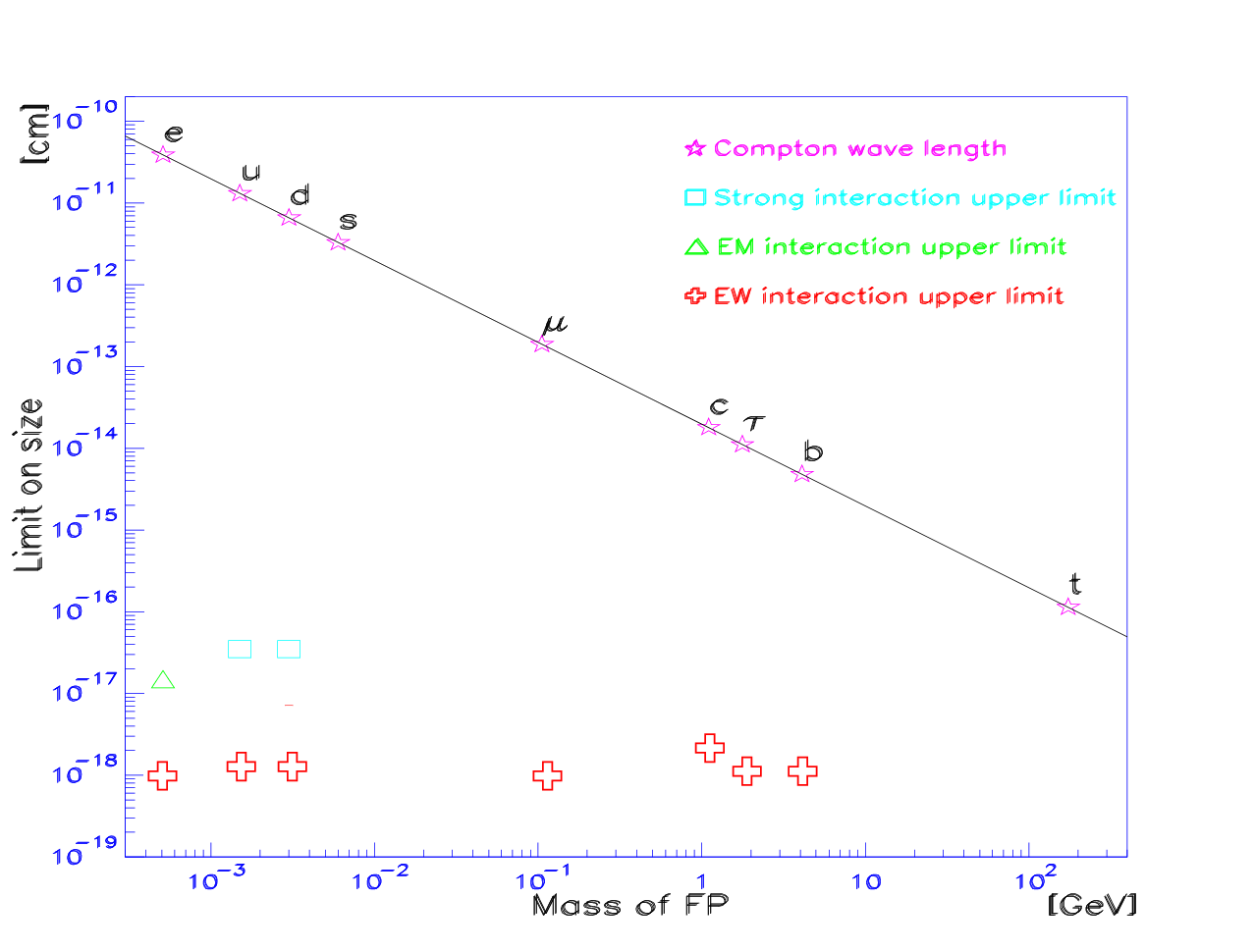
All the limits show that the Compton wavelength is bigger as the characteristic size of the interaction area. This experimental fact is used in section particle-like structure related to gravity to estimate the size of FP and the mass of the Higgs.
3 Cosmology and the early Universe
3.1 Evolution of the universe
Observations suggest that the universe at large scales is homogeneous and isotropic. To quantify the idea of homogeneity one can calculate for example the mass of a sphere of radius at different locations of the universe. In a strictly uniform Universe with density , one will always get the mass to be . In reality, we will obtain different values when the sphere is centered at different locations so that there will be a fractional rms fluctuations around the mean mass . If this quantity decreases with and becomes sufficiently small for large R, then it makes sense to assign the universe as a smooth at large scales with mean density . In our universe, at 22 2 . and decreases roughly as at larger scales.
This suggests that we can model the universe as made up of a smooth background with an average density being, at best, only a function of time superposed with fluctuations , which are large at small scales but decreases as scale increased. So, at sufficiently large scales, the universe may be treated as being homogeneous and isotropic with a uniform density.
A simple form of a large scale motion of an object located at point consistent with the idea of isotropy can be given as . An observer at the origin will see all particles moving with a speed proportional to the distance from him. Another observer located at will see the object at to move with the velocity so that are also moving away with a speed proportional to the distance from the observer 33 3 Here and further on in this chapter we consider a nonrelativistic context of velocity addition.. Integrating this relation, , we can describe the position of any material body in the universe in the form where is a scale factor related to by and is a constant for any given material body in the universe. It is convenient to call and the comoving and proper coordinate of a body and the expansion (scale) factor. Therefore the dynamics of the universe is entirely determined by the function . The simplest choice would be to make a constant, which would imply no motion in the universe and all matter would be distributed uniformly in a static configuration. However, it is clear that such a configuration should be violently unstable when mutual gravitation forces of the bodies are taken into account. Any such instability will eventually lead to random motion of particles in localized region thereby destroying the initial homogeneity. Observationally, however, is indicated that the relation does hold in our universe with .
The dynamics of can be understood from the application of general relativity to a homogeneous and isotropic distribution of matter with interpreted as the energy density. Indeed, in the case of a homogeneous and isotropic spacetime, the interval obeys a particular simple form:
| (27) |
where the parameter modifies the metric of 3-space and the function scales the distances between any two points in the 3-dimensional space. One of the Einstein’s equations then reduces to
| (28) |
while the rest of the equations are satisfied if the equation of motion for matter are satisfied.
Observations suggest that our universe today 44 4 We will refer to quantities evaluated at the present time epoch with a subscribe zero. is governed by Eq.28 with
| (29) |
where ranges from to . The relation is known as Hubble’s law and is called Hubble’s constant. Using one can construct the time scale and the length scale ; characterizes the evolutionary time scale of the universe and is of the order of the largest length scale currently accessible in cosmological observations. A common value to describe the evolution of the universe is the deceleration parameter of Eq.30
| (30) |
More importantly, one can also construct out of a quantity with the dimension of density called critical density
| (31) |
It is useful to measure all other mass and energy densities in the universe in terms of critical density defining the ration , where is the mass or energy density associated with a particular species of particles. The parameters used so far to describe the evolution of the universe are summarized in Tab. 9.
| parameter | value |
|---|---|
| Hubble constant | Mpc-1 |
| Evolutionary time | yr |
| Length scale | Mpc |
| critical density | gr cm-3 |
| critical density | Mpc-3 |
| critical density | eV cm-3 |
| critical density | photons cm-3 |
| parameter h |
The numerical value of can absorbed into the definition of by rescaling it so that we can treat as having one of the three values . The choice among these three values for is decided by Eq.28 depending on whether greater than, equal or less than unity. The fact that is proportional to the total energy of the dynamical system described by Eq.28 shows that will have a maximum value followed by a contracting phase to the universe if , . The Tab. 10 summarize the three possibilities.
| deceleration | curvature | density | |
|---|---|---|---|
| monotone increasing | |||
| monotone increasing | |||
| final cyclic |
If a light was emitted at and received today (when ), the wavelength will change by the factor , where is called the redshift corresponding to the epoch of emission, . Thus, one can associate a redshift to any epoch by . It is very common in cosmology to use as a time coordinate to characterize an epoch in the past.
To determine the nature of the cosmological model we need to know the value of for the universe, taking into account all forms of energy densities existing at present. In particular, to determine the form of from Eq.28 we need to determine how varies with . As a particular species contributes an energy density and pressure one needs to integrate the equation of motion 66 6 The equation reflects thermodynamical relation with . to determine the behavior of with respect to . The simplest equation of state which is adequate in describing the large scale dynamics of the universe is . Then the equation
| (32) |
can be immediately integrated to give . Doing that for each component of the energy density, Eq.28 can be written in the form
| (33) |
where each of the species is determined by density parameter and the equation of state characterizing by constant . The most familiar forms of energy densities are those due to pressure less matter (dust) or radiation. For the dust we have , while for radiation .
Observation situation regarding the composition of our universe can be summarize as follows.
Our universe has or, more precisely, . The value is determined from the angular anisotropy of CMBR., with reasonable assumption . This observations now show that we live in a universe with density close to the critical density.
Measurements of primordial; deuterium produced in the BBN as well as the CMBR observations show that the total amount of baryons in the universe contributes about . Given the independent observations on the Hubble constant which fix , we conclude that ranges between 0.01 and 0.06. Therefore most of the universe is non-baryonic.
Host of observations related to the large scale structure and dynamics (such as rotation curves of galaxies, estimate of cluster masses, gravitational lensing, galaxy surveys) all suggest that the universe is populated by a non-luminous component of matter, the dark matter (DM), made of weakly interacting massive particles which does cluster at galactic scales. This component contributes about .
Combining the last observation with the first one described above we conclude that there should exist at least one more component to the energy density of the universe contributing about 70% of the critical density. Early analysis of several observations indicated that this component is unclustered and has negative pressure. This is confirmed dramatically by more resent supernova observations and analysis of CMBR data obtained by WMAP. The observations suggest that the missing component, the dark energy (DE), has
and contributes .
The simples choice for the dark energy is a fluid with such that . In this case, the equation Eq.32 is identically satisfied with . That is a fluid, which will have the same energy density and pressure at all the time as the universe expands 77 7 This is to be contrasted with the energy density of normal matter which decreases as the universe expands, because of the work done by term with . When the pressure is negative, the decrease in the energy density due to expansion can be compensated by the negative work done thereby maintaining constant energy density.. It is indeed possible to mimic such a fluid by adding a term to Eistein’s equations called the cosmological constant. It is also possible that the energy of the vacuum state of the universe is non zero and exerts a gravitational influence. One should expect that the vacuum have an energy density and pressure which are constant in space and time. The equation Eq.32 then demands that it should have an equation of state . Hence one often calls the dark energy arising from a fluid with equation of state either as cosmological constant or vacuum energy.
The universe also contains radiation (with ) contributing an energy density today most of which is due to photons in the CMBR 88 8 Assuming that most of the energy density is at temperature today, we get . Dividing this by we get the density above..
Taken together we conclude that our universe has (approximately) , , , . All known observations are consistent with such an admittedly weird composition for the universe. Tab. 11 summerizes the numerical values of the experimental measured parameters for the Hubble parameter and density composition of universe.
| parameter | Symbol | value |
|---|---|---|
| Hubble parameter | h | |
| Total matter density | ||
| Baryon density | ||
| Dark matter density | ||
| Dark energy density |
As far as dynamics concerned, we therefore need to consider three form of energy densities: , and . If neither particles nor photons are created or destroyed during the expansion, then their number density will decrease as as increases. In the case of photons, the wavelength will also get stretched as . Thus energy density of material particles scales as , while that of radiation vary as . The latter means that as we go to smaller in the past, radiation energy density grows faster (as ) compared to matter energy density (which grows as ). So even though radiation is dynamically irrelevant today, it would have been the dominant component in the universe at sufficiently small : when . That is at redshift larger than
| (34) |
Further, combining with the result for thermal radiation, it follows that any thermal spectrum of photons in the universe will have its temperature varying as . In the past, when the universe was smaller, it would also have been denser, hotter and, at sufficiently early epochs, was dominated by radiation energy density since .
Given all this, the total energy density in the universe at any epoch can be expressed as
| (35) |
where and various ’s refer to their values at . From Eq.33 we get
| (36) |
This equation can be cast in a more suggestive form. Namely one can introduce a dimensionless time coordinate . Then writing and one obtains
| (37) |
where
| (38) |
Eq.37 has the structure of the first integral for motion of a particle with energy in a potential . For models with we can take so that . Then the dynamics of the system can be classified as follows: (i) At high redshift (small q) 99 9 For the notations chosen . the universe is radiation dominated and velocity is independent of the other cosmological parameters. (ii) At lower redshift () the universe is matter dominated. (iii) At still lower redshift () the velocity changes from being a decreasing function to an increasing one. In the other words, the presence of a cosmological constant leads to an accelerating universe at low redshift.
Based on the above considerations, we can identify three distinct phases in the evolution of the universe depending on which form of the energy density dominates the expansion. At very early epoch, the radiation will dominate over other forms of energy densities and Eq.37 can be easily integrated to give . As the universe expands, a time will come when (, Eq.34) the matter energy density becomes comparable to radiation energy density. Similarly, at very late epochs, the vacuum energy density (cosmological constant) will dominate over non relativistic matter and the universe will become ”vacuum dominated”. This occurs at a redshift of . For , this occurs at . During , the universe is matter dominated with .
Basically it is possible to distinguish eight time intervals summarized in Fig.14. From t=0 to t=10-43 s the Planck Era, at t=10-35 s the GUT Era, at t=10-10 s the Electroweak Era, at t=0.001 s the Particle Are, at t=3 min the Era of nucleon synthesis, at t=300 000 a the Era of Nuclei, at 1 billion years Era of Atoms and until today the Era of galaxy formation.
3.2 Key events in the life of the universe
3.2.1 Overview and present status of inflation
Inflation was introduced to solve several outstanding problems of the standard Big Bang model [68] and has now become an important part of the standard cosmology. It provides a natural mechanism for the generation of scalar density fluctuations that seed large scale structure, thus explaining the origin of the temperature anisotropies in the cosmic microwave background (CMB), and for the generation of tensor perturbations (primordial gravitational waves) [69, 70, 71, 72, 73].
A distinct aspect of inflationary perturbations is that they are generated by quantum fluctuations of the scalar field(s) that drive inflation. After their wavelength becomes larger than the Hubble radius, these fluctuations are amplified and grow, becoming classical and decoupling from causal microphysical processes. Upon re-entering the horizon, during the radiation and matter dominated eras, these classical perturbations seed the inhomogeneities which generate structure upon gravitational collapse [70, 72, 73]. A great diversity of inflationary models predict fairly generic features: a gaussian, nearly scale invariant spectrum of (mostly) adiabatic scalar and tensor primordial fluctuations, which provide an excellent fit to the highly precise wealth of data provided by the Wilkinson Microwave Anisotropy Probe (WMAP)[75, 76, 77] making the inflationary paradigm fairly robust. Precision CMB data reveal peaks and valleys in the temperature fluctuations resulting from acoustic oscillations in the electron-photon fluid at recombination. These are depicted in Fig.11 where up to five peaks can be seen.
Baryon acoustic oscillations driven by primordial fluctuations produce a peak in the galaxy correlations at Mpc (comoving sound horizon) [74]. This peak is the real-space version of the acoustic oscillations in momentum (or ) space and are confirmed by large scale structure (LSS) data [74].

Perhaps the most striking validation of inflation as a mechanism for generating superhorizon fluctuations is the anti correlation peak in the temperature-polarization (TE) angular power spectrum at corresponding to superhorizon scales [75] and depicted in Fig.12. The observed TE power spectrum can only be generated by fluctuations that exited the horizon during inflation and re-entered the horizon later, when the expansion of the universe decelerates.


The confirmation of many of the robust predictions of inflation by current high precision observations places inflationary cosmology on solid grounds.
Amongst the wide variety of inflationary scenarios, single field slow-roll models provide an appealing, simple and fairly generic description of inflation. Its simplest implementation is based on a scalar field (the inflaton) whose homogeneous expectation value drives the dynamics of the scale factor, plus small quantum fluctuations. The inflaton potential is fairly flat during inflation and it dominates the universe energy during inflation. This flatness not only leads to a slowly varying Hubble parameter, hence ensuring a sufficient number of efolds of inflation, but also provides an explanation for the gaussianity of the fluctuations as well as for the (almost) scale invariance of their power spectrum. A flat potential precludes large non-linearities in the dynamics of the fluctuations of the scalar field.
The current WMAP data are validating the single field slow-roll scenario [75, 76, 77]. Furthermore, because the potential is flat the scalar field is almost massless, and modes cross the horizon with an amplitude proportional to the Hubble parameter. This fact combined with a slowly varying Hubble parameter yields an almost scale invariant primordial power spectrum. The slow-roll approximation has been recently cast as a systematic expansion [78], where is the number of efolds before the end of inflation when modes of cosmological relevance today first crossed the Hubble radius.
The observational progress begins to discriminate among different inflationary models, placing stringent constraints on them. The upper bound on the ratio of tensor to scalar fluctuations obtained by WMAP convincingly excludes the massless monomial potential [75, 76, 77] and hence strongly suggests the presence of a mass term in the single field inflaton potential [79, 80]. Hence, as a minimal single field model, one should consider a sufficiently general polynomial, the simplest polynomial potential bounded from below being the fourth order trinomial potential [81].
The observed low value of the CMB quadrupole with respect to the CDM theoretical value has been an intriguing feature on large angular scales since first observed by COBE/DMR [82], and confirmed by the WMAP data [76, 77]. In the best fit CDM model using the WMAP5 data we find that the probability that the quadrupole is low or lower than the observed value is just 0.031. Even if one does not as care about the specific multipole and looks for any multipole as low or lower than the observed quadrupole with respect to the CDM model value, then the probability remains smaller than 5%. Therefore, it is relevant to find a cosmological explanation of the quadrupole suppression beyond the CDM model.
3.2.2 Primordial nucleosynthesis
When the temperature of the universe was higher than the temperature corresponding to the atomic ionization energy, the matter content in the universe was a high temperature plasma. For , in the radiation dominated phase, ; therefore
| (39) |
where counts the relativistic degrees of freedom. As the temperature decreases, more and more particles become non-relativistic; thus is a slowly decreasing function of . Numerically,
| (40) |
When the temperature of the universe is higher than the binding energy of the nuclei (), none of the heavy elements (helium and metals) could have existed in the universe. The binding energies of the first four light elements, , , and are 2.22 MeV, 6.92 MeV, 7.72 MeV and 28.3 MeV respectively. This would suggest that these nuclei could be formed when the temperature of the universe was in the range between 1 and 30 MeV. The actual synthesis takes place only at a much lower temperature, . The mean reason for this delay is the ’high entropy’ of our universe, i.e., the high value of the photon-to-baryon ratio, , given as:
| (41) |
The nucleosynthesis requires protons and neutrons combining together to form bound nuclei of heavier elements like deuterium, helium etc.. The abundance of these elements are going to be determined by the relative abundance of neutrons and protons in the early universe. Therefore one needs first to worry about the maintenance of thermal equilibrium between protons and the neutrons. As long as the inter-conversion between and through the weak interaction processes: , and the decay , is rapid compared to the expansion rate, thermal equilibrium will be maintained. Then the equilibrium ratio will be
| (42) |
where . Therefore, at high () temperature, there will be equal number of neutrons and protons but as the temperature drops below about 1.3 MeV, the neutron fraction will start dropping exponentially provided thermal equilibrium is still maintained. The expansion rate Eq.39 at is given by . The neutron to proton conversion rate, for example, is well approximated by
| (43) |
Therefore, at , this gives , slightly more rapid than the expansion rate. As drops below , this decreases rapidly and the reaction ceases to be fast enough to maintain thermal equilibrium. Using the rate equation, which is the basis of the general procedure for studying non equilibrium abundances in an expanding universe, one arrive to the conclusion that the neutron fraction falls out of equilibrium when temperatures drop below 1 MeV and it freezes to about at temperatures below 0.5 MeV.
As the temperature decreases further, the neutron decay with a half life of becomes important and starts depleting the neutron number density. The only was the neutrons can survive is through the synthesis of light elements. As the temperature falls further to , significant amount of He could have been produced if the reaction rates were high enough. All possible reactions which produce are based on D, and and do not occur rapidly enough because the mass fractions of D, and are still quite small (, and respectively) at . The reaction will lead to an equilibrium abundance ration of deuterium, which passes through unity (for ) at the temperature of about 0.07 MeV which is when the nucleosynthesis can really begin.
Therefore, one needs to determine the neutron fraction at given that it was about 0.15 at 0.5 MeV. During this epoch, the time-temperature relationship is given by . The neutron decay factor is for . This decreases the neutron fraction to at the time of nucleosynthesis. When the temperature becomes , the abundance of and builds up and these elements further react to form . A good fraction of D and is converted into . The resultant abundance of can be easily calculated by assuming that almost all neutrons end up in . Since each nucleus has two neutrons, per unit volume of helium nuclei can be formed if the number density of neutrons is . Thus the mass fraction of will be
| (44) |
where is the neutron abundance at the time of production of deuterium. For , giving . Increasing baryon density to will make . An accurate formula for the dependence of helium abundance on various parameters is given by
| (45) |
where measures the baryon-photon ratio today via the relation
| (46) |
and is the effective number of relativistic degrees of freedom contributing to the energy density and is the neutron half life.
As the reactions converting D and into proceed, the number density of D and is depleted and the reaction rates- which are proportional to - become small. These reactions soon freeze-out leaving a residual fraction of D and (a fraction of about to ). Since it is clear that the fraction of (D, ) left left unreacted will decrease with . In contrast, the synthesis, which is not limited by any reaction rate, is fairly independent of and depends only on the ration at . The best fits, with typical errors, to deuterium abundance calculated from the theory, for the range reads
| (47) |
The production of still heavier elements, even those like , which have higher binding energies than , is suppressed in the early universe. Two factors are responsible for this suppression: (1) For nuclear reactions to proceed, the participating nuclei must overcome their Coulomb repulsion. The probability to tunnel through the Coulomb barrier for heavier nuclei (with large ) is suppressed. (2) Reaction between helium and proton would have led to an element with atomic number 5 while the reaction of two helium nuclei would have led to an element with atomic mass 8. However, there are no stable elements in the periodic table with
The current observations indicate, with reasonable certainty that: (i) . (ii) and (iii) . These observations are consistent with the predictions if , and . Using , this leads to the important conclusion: . When combined with the broad bound on , , say, we can constrain the baryon density of the universe to be . It shows that, if then most of the matter in the universe must be non baryonic.
Since production depends on , the observed abundance of restricts the total energy density present at the epoch of nucleosynthesis. In particular, it constraints the number of light neutrino 1010 10 That is, neutrinos with which would have been relativistic at ).. The observed abundance is best explained by , is barely consistent with and rules out . As we have mentioned in the previous chapter, the laboratory bound on the total number of particles including neutrinos, which couples to is , which is consistent with the cosmological observations.
The major events since Big Bang are summarized in Fig.14

4 Summary of experimental status of Standard and Big Bang Model
The Standard Model is defined by 19 parameters and in the Big Bang models for e.g. in the CDM case by 11 basically cosmological parameters [76, 67, 83]. Both theories are extensively experimental tested and proven to describe our nature. The quantized SM model is applicable in particular at small distances describing the fundamental particles and the interaction between them whereas the Big Bang Model describes distances from the Planck Scale up to size of the universe today. We like to stress that both theories can describe only one nature. The logically consequence about this fact is that between both theories similarities or links must exist.
In Tab. 12 we discuss these links in more detail. The Dirac equation and the Einstein equation are examples of the principle equations in both theories. The are embed in the same four dimensional space and use the same definition of energy E. To calculate radiative effects for example in the reaction Eq.21 it is necessary to introduce a vacuum which allows virtual corrections. The experimental evidence of this corrections is for example visible in the differential cross section of the reaction in Fig.7 where the measured data prefer the level. In a microscopic picture the vacuum produces for example statistical virtual particles and anti-particles like a flashing volume. Similar statistical properties are needed in the Big Bang theory to explain the small temperature fluctuations on the micro wave background of the actual WMAP experiment [84]. It seems for this reason very likely both vacuum used in the Standard ( SM ) and Big Bang Model ( BBM ) are the same. The generation of mass is performed in the SM via the Higgs mechanism. In the BBM produces every stress energy tensor an curved space what means mass. As for all four interactions an tensor exist mass will be produced accordingly these interactions. Similar as the mass generation also for the momentum both theories a very different. The SM momentum follows the quantized regime and the BBM the classical ansatz. The most remarkable difference is that the SM uses the wave function to localize the probability of a coordinate of a particle whereas such an approach in the Big Bang model is absent. A mass accumulation in this model must be described by particle density and the coordinates . It seems very unlikely that the size of a particle in the SM with finite rest mass is zero, because the mass density of the FP would be . A particle in the BBM is a cluster of mass possible including charges. The validity of the BBM is limited by the quantization of the gravitation by the Planck scale and density . A discussion about a classical particle in the BBM is for this reason only sensible if the size of such a particle is and the density . The charges ( color, EM, weak ) of particles and the adjacent interactions are domiciled in both theories, whereas the BBM includes the most important interaction for this theory the gravity. The coupling , and in the SM model are depending about the energy scale as displayed in Fig.3. An experiment at higher test energy has to respect the change in the coupling, above the Grand Unification scale only one interaction is left until the Planck scale. Above this scale it is assumed that gravitation is dominating. The test energy is not only an energy the uncertainty principle defines an according size of test distance in an experiment. In other words a test of the point like behavior of the FPs to a test distance zero would imply infinite high test energies. For example at energies GeV the experiment has to deal with only one interaction. A similar behavior of scale dependence we find in the BBM in Fig.14 in particular at energies from the up to the Planck scale and above.
The energy scale in this case corresponds simultaneously to size of the universe and the time after Big Bang. This similarity between SM and BBM has the interesting consequence that an increase of our accelerator energies for example at LHC test the conditions in a very early universe.
| Standard model | LINK | Big Bang models | |
| principle equations | – | ||
| parameter | 19 | – | 11 |
| 4 dimensional space | x,y,z,t | yes | x,y,z,t |
| energy ( eV ) | E | yes | E |
| vacuum | V | yes | V |
| mass | Higgs | – | for |
| momentum | – | ||
| particle location | – | x,y,z,t | |
| particle size | – | ||
| particle density | – | ||
| particle charge | color, EM , weak | yes | color, EM , weak |
| particle interaction | strong, EM , weak | yes | strong, EM , weak, gravitation |
| interaction scale | yes |
5 Possible micro structure of Fundamental Particles
The investigation of physics beyond the SM and BBM model was performed in the past with tremendous effort.
1783 John Michell introduced the Black Hole a body so massive that even light could not escape [88]. The black hole has a one-way surface, the event horizon, into which objects can fall, but nothing is able to escape. The Black Holes are still the subject of intense investigations like non static black holes, Einstein-Yang-Mills sphalerons and black holes,vacuum black holes, soliton and black holes, five-dimensional Black Hole, Skyrme black hole, tiny black holes, hairy black holes,cosmic colored black holes and non-abelian black holes [89].
1931 Paul Dirac introduced the magnetic monopole is a hypothetical particle that is a magnet with only one pole. He showed that if magnetic monopoles exist, then it would explain the quantization of electric charge in the universe [90]. Recently calculations of non-Abilian monopols, monopols in BHI-Higgs theory, gravitate lumps, self-gravitating monopols and monopole-antimonoplo pair get published [91].
Since the introduction of the Yang-Mills theory 1954 [14] the theoretical effort increased to search for fundamental particle like structures.
1958 T. Skyrme introduced Skyrmions a mathematical model used to form baryons a subatomic particle [92]. Their topological charge has been identified with the baryon number. The are not individual baryons but coherent states of known baryons and higher resonances on a compact manifold associated with the spin and flavor symmetry group. In recent years extensive theoretical studies about the different parameters of Skyrmions are performed. Skyrmions and their stability [93], vibration energies and excitation [94], calculating the density , mass and size [95], barion nuclei production [96], spin and isospin [97], Skyriome-Black holes [98], Gravitating Skyriom [99], Skyriom stars [100] and monopole-Skyrioms [101]. Various theoretical models are studied like Landau-Lifshits ansatz, Yang-Mills ansatz, Einstein-Skyrme model or condensates, lattices and fluids. Also a scattering of Skyrmions was investigated [102].
1961 Yoichiro Nambu and Giovanni Jona-Lasinio introduce the Nambu–Jona–Lasinio model [103]. The model is a theory of nucleons and mesons constructed from interacting Dirac fermions with chiral symmetry, it is a dynamical model of elementary particles based on an analogy with superconductivity. The dynamical creation of a condensate from fermion interactions inspired many theories of electroweak symmetry breaking, such as technicolor [104], the top quark condensate [105], quark condensate [106] and nonlocal quark model [107].
1968 Rosen introduced a configuration of a charged scalar field that are classically stable against small perturbations [108]. These stable configurations of multiple scalar fields were studied by Friedberg, Lee and Sirlin in 1976 [109]. The name ”Q-ball” and the proof of quantum-mechanical stability come from Sidney Coleman [110]. Recently investigations of spinning Q-balls are published [111].
1984 F. Klinkhamer and N. Manton describe first time a Sphaleron [16] a static solution to the electroweak field equations of the Standard Model of particle physics. A sphaleron is a saddle point of the electroweak potential energy of the surface in three dimensional analytic geometry and it is involved in processes that violate baryon and lepton number. In some theories, at the higher temperatures of the early universe, sphalerons convert an imbalance of the number of leptons and antileptons formed by the first leptogenesis in an imbalance in the numbers of baryons and antibaryons [112]. The main theoretical investigations are electroweak Sphalerons with spin and charge [113], Sphalerons and Strings [114], Sphalerons and Black Holes [115], Sphalerons and vortex rings [116], Sphalerons and Higgs [117] and and QCD Sphalerons [118].
1997 articles of the Dilaton a hypothetical particle in string theory appears. The Dilaton is a particle of a scalar field, connected to gravity. Investigation are performed about the mass of the Dilaton [119], dilatonic Inflation [120], Dilaton and Quantum Cosmology [121], Dilaton and Dark Energy [122] and Dilaton in Einstein-Yang-Mills theory [123].
1997-2008 recent researches of Solitons are published. The soliton phenomenon was first described by John Scott Russell (1808 - 1882) [124]. A soliton is a self-reinforcing solitary wave that maintains its shape while it travels at constant speed. Solitons arise as the solutions of a class of weakly nonlinear dispersive partial differential equations describing physical systems. The play an important role in particle physics. In the last years investigations get performed of non-Abelian Solitons, gravitating and spinning Solitons , Solitons, quark-solitons, sine-Gordon Solitons, anomalous Abelian Solitons and quark-solitons [125].
2000 semiclassical instability of De Sitter space and Black hole pair creation in De Sitter space get published [126]. De Sitter space is the maximally symmetric, vacuum solution of Einstein’s field equation with a repulsive cosmological constant . De Sitter space was discovered 1917 by Willem de Sitter [127].
2004 investigations of excitation of physical vacuum are performed [128]. The vacuum state [129] is the quantum state with the lowest possible energy. The vacuum state contains fleeting electromagnetic waves and particles that pop into and out of existence. In perturbation theory the properties of the vacuum are analogous to the properties of the ground state of a harmonic oscillator. In the Standard Model the non-zero vacuum expectation value of the Higgs field is the mechanism by which the other fields in the theory acquire mass. The uncertainty principle in the form implies that in the vacuum one or more particles with energy above the vacuum may be created for a short time .
In 2007 theoretical solutions for Einstein-Yang-Mills strings and superconducting electroweak strings are presented [130].
Following the commissioning of LEP 1989 initiated all four LEP detectors a program to search for physics beyond the SM, in particular via the reaction about not pointlike behavior of FPs. Induced from the investigation in chap. 2.2, chap. 2.3 and chap. 2.4 our interest get focused to study the possible consequences of a not pointlike behavior of FPs.
In the quantized SM it is absolute sufficient to describe our experimental knowledge in physics with 19 parameters. It is not necessary to use any micro structure of FP. But it is necessary to accept, that a FP like an electron is geometrical a point with a finite mass, charge, spin, magnetic moment and an electric dipole moment. In a microscopic picture the density of FP will be infinite, the charge must be a point, imagining a point with diameter zero what is able to generate a magnetic moment and an electric dipole moment is conflicting with a three dimensional logic space structure. If we trop the condition that the FP must be a point and allow an extended microscopic structure it is possible to avoid these objections in understanding. Such an approach points to the un-quantized BBM.In this model an object with rest mass must be described by a density mass accumulation originated from an stress energy tensor in a finite space. The particle would be already an extended object. We like to stress that both very successfully theories describe the same physical object. For this reason it seems usefully to search for an ansatz of a geometrical extended object in the the transition between SM and BBM.
In the following sections we introduce an Empirical Toy Ansatz about a Microstructure of Fundamental Particles ( ETAMFP ) . We follow first the current knowledge of the running coupling constants of the Standard Model together with the time development of the very early Big Bang theory to develop a microstructure of FPs. Both theories are coupled by a common energy scale which defines according the Uncertainty Principle a size. We assume the time-scale-size development of both theories is stored in the size of a fundamental particle. This implements that the part of the fundamental particles which is close to a diameter zero is liked historical to the highest possible scales of the Standard Model and Big Bang theory, the Planck Scale. This logic forms the extent of the Fundamental Particle from a size zero to the size today. The size of the Fundamental Particles is in this sense the direct consequence of the time development of the Standard Model and Big Bang theory from the time up to the time of nucleosynthesis .
To test the validity of this ansatz we step by step confront this model with the experimental measured parameters describing the FPs and ask is the ansatz able to reproduce these parameters. We first test is the ansatz able to organize all the known fermions and bosons in a common scheme. Next we study the consequences of magnetic and electric dipole moment of FPs about the size. Next we are leaving this empirical ETAMFP ansatz and compare it with the microstructure of a neutral particles and the model for a charged particle [150, 161], which are developed from general theory of relativity. Finally we conclude.
5.1 Empirical toy ansatz about a microstructure of a fundamental particle
As already discussed to test in an scattering experiment small distances for example in the discussed reaction two basic conditions have to be full filled. First it is necessary to perform the test at the correct test energy Eq.1, 7) because the test size is direct inverse proportional to the test energy . Second it is necessary to collect a high amount of events about the reaction under investigation. Including radiative corrections of the SM it is possible to push the test size substantial down, as for example demonstrated in the measurement of the electric dipolmoment of the electron [22]. As the FPs are point particles in the SM model an experimental prove of this fact would require an infinite high test energy or infinite high statistics. Both conditions would pass the Grand Unification and Planck scale because it would be necessary to perform the experiment at such energies or calculate radiative corrections up to these scales. The predictions of the SM and BBM model summarized in Fig.3 and Fig.14 demonstrate that the physics conditions have changed at these scales dramatically.
It is not feasible to test in an experiment this extreme energy conditions or perform it with infinite high number of events. The experimental available energies in planning and performed of the known accelerators are displayed in Fig.15 reaching about 15 TeV and simulate a time after Big Bang of about s. The leading parameters which define the physical conditions in the SM model are the test energy and the scale well demonstrated in Fig.3. Essential in the BBM model are the time after Big Bang Eq.40, the temperature Eq.39 and the scale shown in Fig.14 and Fig.15.
To reconstruct for a certain parameter set in the SM and BBM model the same physical conditions it is essential that both model fulfill time reversed invariance. If an experiment is performed at a defined scale according Fig.15, we measure as a function of this scale always the same physical facts, for example at LEP energies and . This result is not a function of the date the experiment was performed, we measure in spring or autumn always at the LEP scale and . The logical consequence of this experimental fact is, the universe remembers how it was created.

The real experiment was performed by nature itself at the creation of the universe, all the scale and time dependence must be stored in the physical laws of SM and BBM model. The fundamental particles get born in these process. We assume for this reason the same happens during the creation of the FPs. Following this philosophy our empirical toy ansatz about a geometrical microstructure of fundamental particles assumes the development about the size of the FPs from size zero to the size today is a result of the early history of the universe stored in the geometrical extension of the FPs, or the geometrical size of the FPs is a result of the time and size development of the history of the very young universe.
5.1.1 The experimental paradox to measure small distances
The experimental paradox to measure small distances is well documented in the reaction. It is not adequate to increase only the test energy of the experiment to measure smaller distances, parallel the physical parameters what are depending about the energy scale change the conditions for the whole experiment. In this sense the experiment is a race between test size and the scale defining the conditions for the whole experiment.
We like to discuss this paradox in more detail in a gedanken experiment. Beginning with the reaction at LEP is the energy approximately 200 GeV. This is above the production threshold to generate W-boson pairs GeV. In the SM model the energy is located after Fig.3 and Eq.7 at a scale of approximately GeV. Including the high statistic of the reaction is this a test size of cm displayed in Fig.9. At this scale the physical conditions are three families of FPs ( see Tab. 1 and Fig.1, three interactions shown in Fig.2 and Fig.3. It is possible to generate and -bosons. According Eq.7 with increasing test energy the set of parameters will be not change until the Grand Unification scale of approximately GeV. At this scale the three interactions unify depending about the Standard Model or SUSY at different energies or in one energy. Beyond this scale until the Planck Scale only one interaction is left. In this era massive super heavy particles are under discussion. This particles would play an important role in the proton decay [31].
Beyond the Planck Scale of GeV or cm test size the quantized gravitation has to be taken into account. 1955 John Wheeler [131] devised beyond this scale the spacetime foam. The foam is supposedly the foundations of the fabric of the universe [132]. At this scale the uncertainty principle allows particles to be created and annihilate without violating conservation laws, the space shrinks and the energy of the virtual particles increases. According Einstein’s theory of general relativity curves energy spacetime, this suggests the energy of the fluctuations would be large enough to cause significant departures from the smooth spacetime seen at larger scales. These fluctuations could serve as a candidate for the seeds of the primordial perturbations in the cosmic inflation because the Large-Scale Structure of the universe is assumed to form as a result of the growth of initially small density perturbations due to gravitational instability [134]. The character of this foam is still under discussion [133] a possibility the foam could be a condensate was discussed by B.L.Hu [135]. If this is true the gedanken experiment will detect between cm and zero cm a condensate.
We used up to this stage of the experiment only the SM model which only implicit defines a test size via the uncertainty principle. Explicitly shown is the test size of our experiment in particular at this very high scales in the BBM model. In this model the horizon distance or size of the universe in the vicinity of the Planck Scale defines unambiguously an upper limit for the test size of our gedanken experiment, if we request the test size should be causally connected. If we use the link of the common scale between SM and BBM as discussed in Tab. 12 it is possible to repeat the gedanken experiment in the BBM model. For the discussion it is sensible to repeat the experiment starting in the vicinity of the Planck Scale down to the scale GeV and use the timing of the BBM discussed in chap.3 in particular Fig.14. If time reversal invariance holds at the Planck size down to a test size zero we like to stress that every experimental physicist unambiguously will measure at this era a superfluid condensate. Between Planck Era and GUT Era the horizon distance or the size of the universe increases, the experiment will be dominated by one interaction only and mass exist already. The gedanken experiment accordingly will measure one interaction and mass or super heavy massive particles. At the GUT scale the size of the universe is sufficient that suddenly three interactions appear accompanied by three types of charges. In the following Electroweak Era the size of the universe will be big enough to host FPs. The gedanken experiment will measure the three families of FPs including the three interactions as discussed in the chap.2.1. We will stop at this scale our gedanken experiment.
If time reversal invariance holds for the SM and BBM model from the vicinity of the Planck Era to the era today the universe is able to remember how it was created. We like to discuss two scenarios beginning with the Planck Era how this fact could be stored in the universe in more detail, in particular focusing on the extent of FPs:
- •
The condensate in the Planck Era exist only in this era until the Planck scale and disappears after the universe cross this scale. In the GUT Era is get replaced by super heavy particles from the size of the universe . After the GUT Era the regime of the three interaction dominates the universe . No condensate or super heavy particles and no phase transitions energies from the different eras exist at the scale today. The parameters defining the different era act precisely at the energy the universe passes the adjacent scale of the particular phase transition.
- •
In the from the gravitation dominated Planck Era the condensate of this era still exist after the universe passed the phase transition from Planck to GUT Era. Primordial inhomogeneities caused by quantum fluctuations in the Planck Era are able to pass to the GUT Era. As the universe expands down to the GUT scale the horizon distance of the condensate increases but stays inside the GUT size. In the GUT Era the primordial inhomogeneities form an onion like aggregates with an inner condensate kernel and outer mass shell. Hypothetical super heave neutral particles are under discussion in this era. These aggregates would be a candidate for the seeds in the inflation for the generation of scalar density fluctuations ( See chap.3.2 ). The sofar discussed conditions including the super heave neutral particles still exist after the universe passes the GUT scale, inside the size of the universe at this scale. After the GUT scale these aggregates could serve as kernels adding outside three types of charges ( colour, electro magnetic and weak ). The three adjacent interaction strong, electro magnetic and weak become distinct. In particular if the strong force get distinct, it seems this is the cause for inflation. After the universe undergoes the inflation the horizon distance is much bigger as every possible generated elementary particle and every relict size of Planck and GUT scale. With increasing time after Big Bang and decreasing temperature a quark gluon plasma will exist. Protons, neutrons, electrons and neutrinos get generated in a hight temperature plasma. Finally the universe follows the in chap.3.2.2 described regime of Eq.39 to Eq.47. Out of a high temperature plasma, FPs and finally atoms get generated and stable.
In this scenario is the geometrical structure of a Fundamental Particle the direct consequence of the development of the primordial inhomogeneities of the Planck Era up to the era today. Still a relict of the condensate of the Planck Era, the mass shell of the GUT Era and the following charges together with remains of the size of the Planck scale and GUT scale should exist today. After our scenario should this structure exist inside every Fundamental Particle.
In the first scenario no information of the development of the universe would exist today. The conditions would be linked direct to the scale energy and appear in the time after Big Bang.
In the second scenario comparing the Planck Scale at GeV or Planck length cm with the experimental limits of the size of FP in Fig. 9 of approximately cm it is obvious that FPs are not created at this scale. The FPs are magnitudes bigger. But the this scenario traces a possibility from the Planck scale until the scale today how the inner structure of a FP could be described. We use for this reason the second scenario for the further discussion.
5.1.2 The geometrical approach
As just discussed our empirical toy ansatz about a microstructure of a fundamental particle is that particle contain every energy state a cross of its radius which the Universe passed through during its evolution shown in Fig.14. For such a case it is possible to read this microstructure direct from the SM model Fig.3 and the BBM model Fig.14. Using these both figures a schematic development of a geometrical extended FP is shown in Fig.16.

In the middle part of Fig.16 we describe the historical procedure initiated from of Big Bang time about mass density, size, charge distribution a point-like observer would measure following the creation of a fundamental particle. The mass of the universe known today is a composite of baryonic matter, dark matter and dark energy. As all these contributions are created from one origin the discussed procedure should be generic for all three contributions. We concentrated in the following discussion only on the baryonic matter because the FPs are located in this part.
In the upper part schematically displayed is the scale dependence of the coupling of , and as function of the scale of the SM model Fig.3. In the lower part we relate the time development of the Big Bang theory of Fig.14 to the SM model with the according energy states Planck Era, GUT Era and the FP Era.
If the spectator initiates the measurement from the Big Bang time t = 0 to the Planck scale he enters an era our knowledge is very poor, all assumptions have to be taken as highly speculative. With this in mind we introduce some hypothesis. In accordance with our previous discussion the spectator will measure a quantized energy mass condensate, originated from a volume explosion with a density of . In this mass- time dominated condensate the charges color, electric and weak are already existing. The constituents of this condensate at a distance below are in direct contact not able to form an interaction similar the field theory in the SM model. The statistical distributed volume explosion does not introduce a total quantized spin different from zero. The consequences of this assumption will be discussed in the next chap.5.1.3
Next the spectator will cross the domain boundary of the Planck scale at GeV at a distance from the center of cm and enters the era to the GUT scale. Usually nature performs smooth transitions from one era to next. We expect for this reason that the gravitational mass dominated regime changes slowly to the GUT scale. It would be likely that a decreasing mass density get generated forming a mass shell enclosing the mass kernel of the Planck Era. This era is dominated by only one interaction. If it is possible to describe this era already by a field theory of high group [31] a geometrical structure of two particles interacting via a gauge particle would be possible. If the total spin of universe would be zero these particles describing the mass shell could carry a spin which adding to a total spin of zero. All well known spins , and zero which are able to adding vectorial to the total spin zero would be possible. As a further consequence the mass shell with a mass density of could in a geometrical microscopic picture rotate around the Planck kernel.
Next the spectator on its time space journey will cross the the domain wall of the GUT Era at GeV at a mass density . At the Grand unification scale in the time development of the universe the three interaction strong, electro magnetic and weak accompanied by the adjacent three types of charges strong, electro magnetic and weak get dominant. This is shown in the upper part of Fig.16. The interactions are at this scale much stronger as the gravitation and the size of the universe is big enough to host three intepented interactions in the three dimensional space. For the spectator who is concentrated on the particle like aggregates with spin axis, which are carried on from the quantum fluctuations of the Planck Era to this scale, three possible geometrical locations appear to place charges on one coordinate axis. One position at the center and two respectively at the surface of the object. In total positions are possible. As shown in a more detailed view in Fig.17 of the fundamental particle it would be possible to place on the x-coordinate three electric charges, the z-coordinate three colors and on the y-coordinate three weak charges.

The assumed spin axis in Fig.17 allows to distinguish between left and right on one coordinate axis with lead to three position if we assume one position exist as discussed at the Planck era on the Planck kernel. The appearance of the three interactions in the vicinity of the GUT scale occurs in the SM model at three or in the SUSY model at one scale energy. Both theories sharing the fact out of one interaction three interaction get born. It is likely that in the first moment after the GUT scale all three possible charges are in direct contact. With increasing time after the GUT scale the full picture of quantum field theory with FPs and gauge bosons would be formed up. In the direct contact regime the displacement between the charges is tiny, repulsive forces could be superimposed by attractive forces. A superposition of similar strong repulsive and attractive forces opens the possibility at a certain distance from the center of the FP stable geometrical positions could exist, where the different forces balance each other. Such positions would be ideal to place charges. For example the positive electric charge on the right side of the x-axis in such a position would allow via these stability conditions only a second charge opposite on the left side of the x-axis. In such a regime with increasing number of charges the discussed positions are possible. This regime would form an energetic minimum. We will discuss this hypothesis in more detail in the chap.5.1.4.
With increasing time after the Big Bang the universe follows in the SM model the conditions of the running coupling constants discussed in the chap.2.1 and undergoes in the BBM model the inflation with all consequences discussed in the discussed in the chap.3. Concerning about the FPs, the universe is big enough to host all FPs, gauge particles and hypothetical particles already exist before the GUT scale. All these particles would be in our ETAMPF model the outcome of primordial quantum fluctuations already in the Planck Era. In particular important would be scalar density fluctuations that seed large scale structures. The size of the universe will decouple from the size of the FPs. The geometrical size of the universe will increase according the comoving scale but the size of the FPs which is stabilized by the four fundamental forces will be the same. According our ETAMPF model also remains of the Planck Era including Planck size and GUT Era including GUT size will get stable and remain inside the FPs. The character of the condensate transferred from the Planck scale until the scale today including also the size of this condensate today and the conditions of mass shell together with the GUT size will be discussed in more detail in the chap.5.3.
After the universe passed the plasma conditions it will follow the discussed scheme of primordial nucleonsynthesis ( See chap.3.2.2 ). The spectator will cross the energy of the experiments. We determine at this energy the journey of our spectator.
The status of the FP at a scale of about GeV is displayed in the middle of Fig.16 and Fig.17. It is an object with a non rotating mass kernel with a density of what is the heritage of the heavily attenuated Planck density . The kernel carries mass and the three charges color , electric and weak . The size of the kernel radius is the relict of the Planck radius by the time development of the universe. The kernel ends at a domain wall separating the kernel from the rotating mass shell ( Spin ) of GUT Ea with a density of and an outer radius of where again a domain wall exist. The mass density is a heritage of the heavily attenuated GUT scale density and the size is the by the time development of the universe expanded radius at the GUT scale. The locations of the three charges at nine positions are the same as discussed at the object existing at the GUT scale. We could place on the x-coordinate three electric charges , on the y-coordinate three weak charges and on the z-coordinate three colors .
5.1.3 Links between continuous symmetries gravitation and spin
To associate the distributions of the charges and mass of the FPs in Fig.17 with the SM and BBM model we used the running coupling constant of the SM shown in Fig.3 and the space-time evolution of the BBM in Fig.14. Embedded in the continuous symmetries of the four dimensional space-time is more information about the two so fare missing connections to the gravitation and spin of the discussed microstructure of of FPs. We like to discuss, four possible links to associate the gravitational interaction to the time of the four dimensional space-time and discuss later the consequences for the FPs about the local isotropy of the space against rotation ( Spin ).
First at scales below the Grand unification the three interactions strong, electro magnetic and weak appear well separated from each other, because the geometrical size of the universe is sufficient to make them distinguishably from each other. These three interaction are embedded in the space for example described by the Cartesian coordinates x, y and z. But in total exist four coordinates and four interactions. The last possible coordinate is the time. In accordance with our discussion above it would be sensible to connect the time to the gravitational interaction. This would of particular importance in the regime above the GUT scale where the gravitational interaction is dominating but it should also hold at the scale today.
Second we like to stress that an experiment which investigates the center of a SM model point like FP will, meet unambiguously the conditions at the Grand unification scale where the gravitation is not negligible any more and next the the Planck Scale where the gravitation get dominant. At the Planck Scale the Planck conditions of mass, length, time and density of Eq.48, Eq.49, Eq.50 and Eq.51 of the gravitation are absolute crucial.
| (48) |
| (49) |
| (50) |
| (51) |
At these conditions a complete geometrical extended three dimensional FP does not exist because the scale is to high or the test distance to small. But if our assumption is true that the FP has accumulated the history of the SM and BBM in his geometrical structure this implements that the inner part of the FP is dominated by the gravitation and the structure is prevailing one dimensional. As the three dimensional test distance is extreme small below cm again the time would be a good candidate for this dimension.
Third the mass-energy equivalence proposed and interpreted 1905 by Einstein, as a general principle which follows from the relativistic symmetries of space and time, points also to the time as connection the gravitation.
Fourth the uncertainty principle connects again the time to the energy.The energy mass equivalent point again to a connection between time and the gravitation.
We use this four indications to connect in the further discussion of this paper the time to the gravitational interaction.
The local isotropy of the space-time leads in the SM via the Noether- Theorem to the angular momentum conservation and finally to the spin of the FPs existing at the scale today. In the SM is the spin a quantum number to describe one feature of the particle. For the point particle of the SM has the spin no microscopic meaning, because a rotating point with diameter zero is meaningless. If we trop the condition of a point particle and allow an geometrical extension of the FPs like in Fig.17 a rotation of the object is possible and the spin, magnetic moment and electric dipole moment is natural included in the object. From experiments we know that for example the spin axis of an electron is anti-parallel to the axis of the magnetic moment of the electron. For our extended object in Fig.17 implies this that the charge is rotating together with the mass center in the same rotation plane. The geometrical extension of the mass in the center, the position of the charges at generate a classical angular momentum, magnetic moment and electric dipole moment. As we discussed in the geometrical approach, remains the question at which time in the development on the universe the spin appears? The spin is associated with the creation of the mass of the FP because in a microscopic picture only a rotating mass like a gyroscope will lead to a stable spin axis. The mass of the FP is in our ETAMFP model a relic of the time between and the Planck time as Planck kernel and between Plank time and GUT time as mass shell. It seems unlikely that the volume explosion before the Planck time generates a spin because this process is statistical equal distributed over the whole volume of explosion. This would implement that the universe has a total spin zero. But after the Planck scale the universe could be already geometrical extended enough to form a particles with a fined size which direct interact with each other like in the field theory of a high group [31]. If in this case a quantized spin get created two particle with spin interact via a field particle with each other. The spin of the particles involved would be well defined. If we assume like in the SM model the particles carry spin the field particles must carry spin or zero, because only or add to zero. In a self interacting mode with two field particles also higher spins like are possible because . It seems after this discussion reasonable to assume the spin appears in the universe in the time window between Planck and GUT scale.
5.1.4 Forces and stability
As discussed in the geometrical approach the dependence of the coupling constants , and as function from the scale in the SM shown in Fig.3 and the time-size dependence of the same scale in the BBM displayed in Fig.14 contains information about which forces exist at which scale and what is the dependence of these forces about the scale of particle size under investigation.
At the LEP scale at approximately 200 GeV a straight conception about forces and FPs exist. The SM contains the three forces strong, electro magnetic and weak shown in Fig.3 which interact with three families of FPs as shown in Fig.1. Up to the Grand unification scale the forces are sorted after there strength . At this scale at about GeV the three forces get unified in one force. The associated test distance in our discussed gedanken experiment is at this scale so small that the concept of the SM of two geometrical separated FPs interacting via an also geometrical separated gauge boson is questionable. In this case it seems reasonable to assume the interaction is similar to a direct contact term interaction for example used in the Lagrangian Eq.24. Between the Grand unification scale and Planck scale only one force exist above the Planck scale the gravitation is dominating. From the experiment the known FPs are in particular in the case of the electron with a mean life time yr extreme stable. This experimental fact require that the distance dependence of the forces acting in the FPs must lead to highly stable conditions.
The target of the following discussion is to develop a general scenario guided from the experimental facts and the scale-time-radius dependence of the SM and BBM model to imagine a possible radius dependence of the known four forces what could lead to such highly stable conditions.
If we start at a radius in the center of the FP it is necessary to discuss first the radius dependence of the gravitation at distances close to the Planck scale and the Grand Unification scale . If we follow the classical force of the gravitation as function of the distance between to masses in a Schwarzschild [144] vacuum as displayed in Fig.18 ( blue broken line ) the force will be infinite at . Such a behavior will not lead to a stable mass core needed from our experimental knowledge for a FP for example like an electron. The mass core will only be stable if the attractive Schwarzschild force in the environment of will change to a repulsive force like a De Sitter [148] behavior ( Red solid line in Fig.18 ).

In such a case in our direct contact term scenario a repulsive force will lead to a repulsive pressure which get balanced by an attractive pressure generated by the Schwarzschild force. Point SPII in Fig.18 describes such a situation. If the stable radius shown as black circle in Fig.19 get smaller a repulsive force will push the mass core back in the stable position ( left middle red circle broken line in Fig.19).

In the contrary if the stable radius increases the radius get pushed back from a attractive force to the left lower broken line in Fig.19. In conclusion only a De Sitter like vacuum would lead to a stable mass core of the FPs.
Second it is necessary to discuss the unification of the electromagnetic force EM, the color force C and the weak force at the Grand unification radius and the involvement of the gravitation between Planck and Grand unification scale.
Between the radius the SM and BBM predicts one force including one coupling constant and for the three discussed forces appear including the three charges color, electromagnetic and weak. The consequence of this prediction is that the charges should be geometrical located at the vicinity of the radius . For simplicity we assume in the further discussion the charge themselves have a point-like geometrical character.
The attractive-repulsive character of the gravitational force in the environment of was investigated in ref.[148] and ref.[153]. Following the concept to find a possible stable scenario for FPs we assume that all three forces change the attractive or repulsive character like the assumed De Sitter behavior of the gravitation at the radius . Numerous combinations to unify the four discussed forces between are possible. We pick one possible scenario put like to point out that also other scenarios will lead to the same result.
The electromagnetic interaction EM is at distances of repulsive as shown in Fig.18 ( Green solid line ) and we assume between the force will decrease to zero or is very small at . If we unify the EM force with the gravitation as shown in the black solid line upper part in Fig.18 a stable point appears like of the gravitation the repulsive inner core forces balance the attractive forces .
An electromagnetic charge located at would be stabilized geometrical very similar as the gravitational mass core at shown in Fig.19. If the stable radius shown as black circle in Fig.19 get smaller a repulsive force will push the EM charge back in the stable position ( Middle left red circle broken line in Fig.19). In the contrary if the stable radius increases the radius get pushed back from a attractive force ( Lower broken red circle in Fig.19 ). In conclusion a De Sitter like behavior of the EM force would lead to a stable geometrical position of an EM charge at point .
If we choose Cartesian coordinates for the FPs , put the center of the FPs at and locate on the +x-axis at one charge opposite at -x-axis a second stable point will exist because this charge will detect for the distance more as an repulsive force to the first charge because the force will be repulsive for . As the charge appears explicitly at the radius it is likely that the charge already exist at . At approximately the prediction of the SM and BBM is that the gravitation dominates all other forces. Even a very small attractive coupling between mass and the three charges would locate one more stable position for these charges at the geometrical position with maxim mass concentration. According Fig.18 would this be direct in the center of the FPs.
The crossing point in Fig.18 leads to a geometrical not stable regime as shown in Fig.19 right side. The force on the right side middle part will collapse to position and the force will expand the position to at the right side lower part.
The color force C and weak force is attractive at if we assume again a change of character close to to a repulsive force and put it at to zero or very small the unification with the gravitation shown as black line in the lower part of Fig.18 will generate a stable point . The scenario for the week force would be very similar and will be not further discussed. It would be possible to place at point color charges. After the previous discussion of the stability in Fig.19 would also the color charge be stabilized close to . If we put the color charge on the + z-axis at an opposite stable condition would exist on the z-axis because the color force would be for for some distance repulsive to stabilize the second color charge opposite to the first charge. The scenario for the week force would be similar on the last free y-axis.
In conclusion to the discussion of the behavior of the four forces it turns out, that the above scenario generates six stable geometrical positions to place charges at approximately plus one position for each charge in the center of the FPs including a stable mass core. The connection between the three axis of the Cartesian coordinates and the three interactions would be explained be simple geometrical reasons.
5.1.5 The flashing vacuum
The ETAMFP model Fig.17 includes a charge circling a kernel. An accelerated charge will emit electromagnetic radiation. Such an object is losing energy, is not stable with a finite life time. If we consider for example an electron with a life time of yr it is obvious a radiation free path as postulated in the Bohr model [139] must exist. A well known example for a stable geometrical extended object is the Hydrogen atom. In the SM model the probability distribution of an electron in state peaks in the center of the proton but not in a delta function at , similar the half stabel state peaks at a a distance outside the center of the proton. The electron circles the center of the hydrogen atom on a radiation free path, statistical appears and disappears in a certain distance from centers of the hydrogen atom and at the same time generate with these flashes a radiation free path around the center of the hydrogen. To interprete this statistical appearing and disappearing a second state would be necessary to give the electron the possibility to disappear. An approbiate candidate for this state would be the vacuum. The vacuum state [129] is the quantum state with the lowest possible energy. This state is characterized by distinct properties. In perturbation theory for example in the reaction the QED differential cross-section Eq.21 is calculated including radiative effects up to . It contains fleeting electromagnetic waves and particles that pop into and out of existence. The uncertainty principle in the form implies that in the vacuum one or more particles with energy may be created for a time . In the environment of a black hole the vacuum get unstable and loses energy via Hawking radiation [145]. Vacuum fluctuations cause a particle-antiparticle pair to appear close to the event horizon of a black hole. One of the pair falls into the black hole whilst the other escapes. In this quantum tunneling effect a particle-antiparticle pair get screened and one will tunnel outside the event horizon. If the total energy is conserved and this particle escapes from the black hole it will cause and energy or mass loss. The Hawking radiation appears near a black hole with all properties of a black hole in particular a Schwarzschild horizon [144] and a singular gravitational potential. In this case the particle pair get screened. A further scenario would be that not a particle anti-particle pair get created but only one particle oscillates statistical between real state and vacuum state for and backward. In all discussed scenarios the vacuum has the possibility to flash statistical on every geometrical location from time to time. It will also be possible close to a fundamental particle. A FP is after our knowledge not a black hole but discussions on the way a FP could be described by a De Sitter-Schwarzschild geometry a black hole whose singularity is replaced with de Sitter core of some fundamental scale [154, 152, 151]. ( See chap. 6) If the gravitational potential is not singular any more the possibility appears after the stability discussion in Fig.18 that one more vacuum property is possible. The vacuum is fluctuating close to a FP similar to the Hawking radiation put with the difference that one pair partner is not escaping from the FP it just appearing statistical at a certain location whereas his counter-partner stays in the vacuum, similar to a mirror particle in a Dirac sea [147] or it oscillates between real and vacuum state. As in all models unter discussion ( See Tab. 12 ) a vacuum exist, we introduce for this reason as working hypothesis the flashing vacuum [146].
Translated in our ETAMFP model Fig.17 would the previous discussion implement for the classical charge rotating on radius an aggregation of statistical flashing charges located with a certain distribution function in the vicinity of the radius . The quantum of flashes per time together with the distribution function would define the radius , if we assume the charge is geometrical substantial smaller as the FP. The integral summed over all flashes would define the total charge of the FP. If the flashes are collective overlaid be a rotational speed would this be the deeper reason for the magnetic moment and the electric dipole moment. The discussion so far we focused on the electric charge, but in particular in perturbation theory radiative effects including strong, electro magnetic and weak interactions. These implements also the attached charges color, electric and weak in the fluctuations. The vacuum properties are also very important for the Higgs mechanism to create mass for the FPs. For this reason it is very likely that the vacuum is also able to flash in a quantum matter mode. In our ETAMFP model the statistical quantum flashes per time together with the a distribution function would define the density distribution as function of the radius . The total integral would allow to calculate the total mass of the FP and similar as the charges would an overlaid rotational speed of the flashes generate an angular momentum and the integral the total spin. Again the geometrical extension of such a mass quantum must be smaller as the size of a FP. We assume as an ad hoc hypothesis the frequency of these quantum of flashes is high enough that it can be calculated in a classical ansatz. This approach we will follow in the next sections of this paper.
5.1.6 Conclusion of the empirical toy ansatz about a microstructure of a fundamental particle
We first discussed the experimental paradox to measure very small distances. In the case of the point like Standard Model FPs it would be necessary to measure distances down to zero. This unambiguously request infinite high test energies, the CM energy of the experiment will cross the GUT scale and Planck scale. The logic consequence is, the whole physics conditions according to the energy scale of the SM- or BBM-model change to the physics laws existing at this scales. The experiment must be performed below the Planck time of and the Planck length of cm. To reconstruct for a certain scale in the SM and BBM model the same physical conditions it is essential that both model fulfill time reversed invariance. This is confirmed from experiment up to the LEP energies. For our discussion we assume this is correct up to Planck Era. The logical consequence of this fact is, the universe remembers how it was created. In our empirical toy ansatz ETAMFP about a microstructure of a fundamental particle we propose that the FPs contain every energy state a cross of its radius which the Universe passed through during its evolution. In this scenario is the geometrical structure of a Fundamental Particle the direct consequence of the development of the primordial inhomogeneities of the Planck Era up to the era today. Still a relict of the condensate of the Planck Era, the mass shell of the GUT Era and the following charges together with remains of the size of the Planck scale and GUT scale exist today inside every Fundamental Particle. The ETAMFP model changes the point like FPs of the SM to geometrical extended objects. It follows the evolution of the universe in the BBM model in particular the primordial nucleosynthesis, but the FPs are not points any more.
Second we developed an approach of a geometrical extended fundamental particle. We use the obvious proposal that the SM and BBM describe the same nature and use the common link of the scale between both models. This links the scale dependence of the couplings of the SM model , and together with the time after Big Bang. In this case it is possible to read the microstructure of the FPs, as a remain of the time development of the early universe direct from the SM and BBM model in three major steps. At the time window a condensate of mass and the three charges color, electromagnetic and weak get created including the geometrical size of the phase transition Planck to GUT Era, between mass creation dominates the geometrical size of the phase transition GUT to era today get stored and finally at the window the primordial inhomogeneities carried over from the Planck Era get equipped with the three charges color, electromagnetic and weak according the three accordingly interactions strong, electro magnetic and weak. The whole structure follows the inflation and ends at the FP Era as fundamental particles.
Third we discussed links between continuous symmetries gravitation and spin. After the discussion of four possible links to associate the gravitational interaction to the time of the four dimensional space-time we conclude that the three interactions strong, electro magnetic and weak are dominant in the three dimensional space and the fourth interaction the gravitation is linked the time. Following the timing of the the SM- or BBM-model we assume the spin appears in the universe in the time window between Planck and GUT scale.
Fourth we search for a link between forces acting inside a FP and its stability. As for example the electron is a highly stable particle the radius dependence of the forces inside the electron must lead to a very highly stable condition. It turns out that only stable conditions are possible if the known forces strong, electro magnetic, weak and gravitation change from repulsive to attractive or vice versa close or inside the FP where the strength of the gravitational force is similar or even dominating. The discussion about the radius behavior of the four forces shows that the above scenario generates six stable geometrical positions to place charges at approximately plus one position for each charge in the center of the FPs including a stable mass core. The geometrical locations of the different charges would be explained be simple geometrical reasons and a energy minimum of the FP mass.
Finally fifth we investigate the question, why the rotating highly accelerated charge of the ETAMFP model does not radiate electro magnetic energy? We conclude from the electron with a life time of yr a radiation free path similar postulated in the Bohr model must exist. We use the stable Hydrogen atom to search for a microscopic picture how an electron in a p-state is able to circle the center of the Atom without radiation. We introduce the flashing vacuum as candidate to give the electron the possibility to appear and disappear statistical to form the well known probability distribution . We extend the in the SM and BBM model defined vacuum properties by the possibility the vacuum is fluctuating close to a FP similar to the Hawking radiation put with the difference that one pair partner is not escaping from the FP it just appearing statistical at a certain location, whereas his counter-partner stays in the vacuum, similar to a mirror particle in a Dirac sea or it oscillates between real and vacuum state. For a working hypothesis we assume the frequency of quantum flashes is big enough that we can use it for a classical ansatz of a radiation free path of the charges circling around the center of the FP.
The geometrical structure in our ETAMFP model is generic every extended stable or semi stable structure originated from the primordial inhomogeneities or quantum fluctuations in the Planck Era are fundamental. In the introduction of chap.5 we summarized the main various structures what are under discussion today. All the discussed particle like structures should be indicated as fundamental particles. To simplify the discussion in the followings chapters we like to follow the common habit to restrict the name of fundamental particles to fermions, bosons and higgs.
5.2 Scheme of geometrical extended fundamental particles and anti-particles
To confront the ETAMFP model of an geometrical extended FP described in Fig.17 we test first is the model able to sort all known fundamental particle ( Fermions ), fundamental anti-particle ( Anti-fermions ) and interaction particles ( Bosons ) in one common scheme.
5.2.1 The charges of fundamental particles
After the experiment of R. A. Millikan (1911) [32] we learned from experiment most of fundamental particle carries charges. The charges of the FPs of the four interactions assigned in Fig.2 localize geometrical the location of the source of the interaction and the strength of the strong, electromagnetic, weak and gravitational interaction.
A) The charge of the strong, electromagnetic and weak interaction.
To test the scheme it is first necessary to summerize the charges of the standard theory at a low scale at about as displayed for example in Fig.3. The strong interaction is described by the three charges red ( R ), green ( G ) and blue ( B ). The most fundamental charge of the electromagnetic interaction is . The charge of the weak interaction is the weak isospin and . The hypercharge quantum numbers is a function of the electric charge and the weak isospin according Eq.52.
| (52) |
B) The pseudo charge of the gravitational interaction.
The model in Fig.17 describes so far in three dimensions how to place on the x-axis the electromagnetic charge , on the y-axis the weak charge and on the z-axis the color charge . As we know that the SM and BBM model uses four dimensions it is essential to study which type of charge belongs to the fourth dimension the time. After we discussed in the chapter about links between continuous symmetries gravitation and spin we reached the conclusion to link in this paper the time to the gravitational interaction. Two indications point to the mass as pseudo charge of the gravitational interaction.
First we consider the definition of a charge as source of a force field in field theory. The field in the environment of a charge contains energy. If we investigate the Einstein equation in Tab. 12 and ignore for the discussion the cosmological term energy will implement energy stress tensors . It means also the curvature will be not zero. As consequence in the environment of the charge after the Einstein equation mass must exist. If we assume a charge is the source of a force field and the Einstein equations are valid for our case a charge can not exist without mass. The fact is unique for all known charges color, electric and weak. As consequence fundamental particles ( fermions and bosons ) which carry on type of this charge must also carry mass.
A special case is the mass them self in the Einstein equations. If we extent the definition of a charge as source of a gravitational field on the mass, the mass get a double significance. The mass would behave just as mass in ( gr ) in our usually definition but would be at the same time a charge like the color, electric and weak charge. This self interacting phenomenon will equip every spatial energy accumulation of a field with mass, in particular the gamma and Higgs. The gamma is a hybrid because it is a spatial energy accumulation of electromagnetic character, it carries via induced mass and is electromagnetic. It is sensitive via the induced mass to gravitational interaction and the gauge particle for the electromagnetic interaction.
These considerations unify the known four interactions strong, electro magnetic, weak and gravitation with four charges color, electric, weak and mass to one scheme and at the same time connect the four interactions and charges to the four coordinates as discussed in the chapter geometrical approach.
Second is the mathematical structure of the forces between two charges and in the Coulomb law Eq.53,
| (53) |
the force between two magnetic poles and Eq.54
| (54) |
and the the gravitational force between two masses and Eq.55
| (55) |
absolute analog. But the analogy between the charges , , and the mass is not general valid. For example is the amount of the electric charge not depending about the velocity if the FPs in contrary to the rest mass of the particle which follows the Lorentz-Transformation, which pushes the mass to infinite if the velocity of the particle approaches the velocity of light.
For a working hypothesis we use in the following discussion of this paper the mass as pseudo-charge of the gravitational force. The extention of the FP can be originated from the size of the mass kernel and/or the size of the color, electric and weak charge. Without limiting the general discussion we assume that the color, electric and weak charge is point-like and the whole extention of the FP is originated from the density distribution of the mass as function of time , radius and the geometrical position the charges , and of the FPs get placed.
C) Effect of charges for a geometrical extended object.
An electric charge located at the border of an extended object with spin will generate a magnetic moment and under certain conditions an electric dipole moment. Inspecting the basic scheme of a FP in Fig.17 it is possible to assume the principle for the electric charge is also correct for the color, weak and mass charge. This assumption would have the consequence that the four charges generate four moments and for dipole moments. Originated from the color charge a color moment, from the electric charge a magnetic moment, from the weak charge a weak moment and from the mass a mass moment. The same charges are able to generate the equivalent color-, electric-,weak- and mass-dipole moment. The FPs carry usually not only one charge for example in the quark case color, electric, weak and mass charge. This would lead to the the possibility of mixed moments and dipole moments.
So fare experimental evidence exists for the magnetic moment of the electron and muon [137] and a hint about the electric dipole-moment of the electron and muon [137]. In addition experimental limits and discussions about quark color magnetic moments and weak magnetic moments are on the way [141]. The introduced scheme in Fig.17 respects the experimental knowledge we have today. The color charges on the spin axis ( z-axis ) would generate a small or zero color moment, the electric charges on the x-axis would generate a magnetic moment and the weak charges on the y-axis would generate a weak moment. According Fig.17 we assume for the mass a geometrical distribution of a mass density together with the spin-rotation will this generate an angular momentum the spin. It will not generate a mass-dipole moment unless the mass distribution is geometrical somehow clustering. In the Einstein equations a mass-dipole moment is forbidden, which implements the assumption the mass density distributions is not clustering.
5.2.2 Extension of the geometrical approach to four dimensions
To extend the three-dimensional scheme of Fig.17 to four dimensions, we introduce the scheme for an electron in Fig.20. The three Cartesian coordinates are assigned at the left side of the figure by black solid lines. Left of the line are written down the three coordinates x, y and z and on the right the attached charges , and . The fourth coordinate is shown on the right side. Left the time and right the pseudo charge mass. The geometrical center of the FP is a green dot. The geometrical position of the charges , and is symbolized by the length of the black line. Above the black line for a coordinate is shown the amount of the charge at the position left, center and right in blue numbers. The integral of the charge measured far away from the FP is shown below the black line in red color. The common used symbol for the FP is displayed in the center of the figure above a big red dot. The time coordinate on the right side of the scheme has only a center ( gree dot ) and a black line to right, symbolizing the fact that negative absolute time does not exist. Above the black line a mass is assigned in blue color if the particle is stable. Below a mass is assigned if the particle has a rest mass. Mass assigned means matter and means antimatter. The length of the black time line symbolizes that the FP has a mass. We do not distinguish between rest mass and energy.
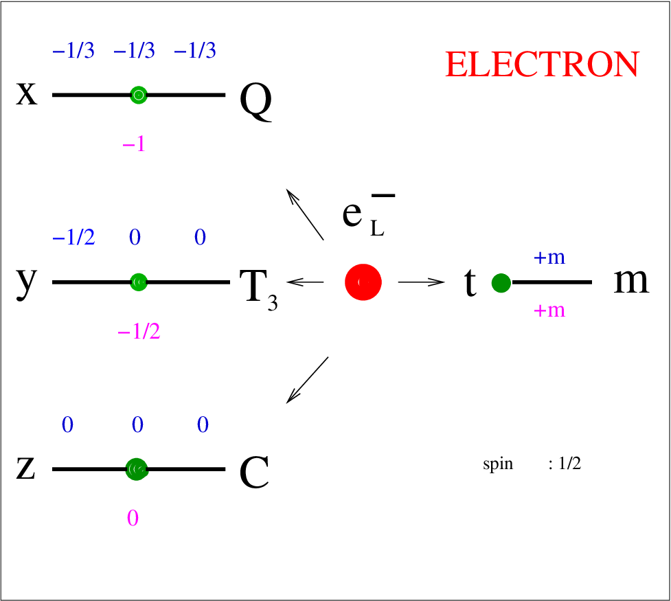
Before we apply the scheme on all FPs we demonstrate how to use the scheme to describe for example an electron in detail as shown in Fig.20. At the scale four independent interactions exist and four orthogonal coordinates are available. Following the discussion of section, empirical toy ansatz about a microstructure of a fundamental particle, the mass kernel of the FP will be time like and the strong, electromagnetic and weak interaction space like. The spatial extended mass kernel together with the spin of the FP assigns for every axis three distinguished positions to place a point like charge, as shown in Fig.17. Two at the border of the mass kernel and one in the kernel. The spin axis of the FP we coincide as distinguished axis with the z direction. As discussed we keep the z-axis free for the color charge, place the weak charge on the y-axis and place the electric charge on the x-axis. The electron carries no color charge which sets the charge on the z-axis to zero. The weak hypercharge ranges from to and is according Eq.52 a function of the charge and the weak isospin which ranges from to in units of . These number is more fundamental and for this reason used as quantum number for the discussed scheme. We have the possibility to place the weak charges what could be , and on the y-axis. In case of the electron . Three possible positions left center and right are open. If the electron would carry a weak moment it would be necessary to put the charge left or right of the y-axis. As this is not excluded so far we use the position y-axis left. The total charge measured from far outside the electron would be also . The electric charge must be placed on the x-axis or y-axis because only in this position it is possible to generate together with the spin a magnetic moment and electric dipole moment. We choose the x-axis. On the x-axis all the three open positions will be occupied with . The total charge measured from a spectator far outside the mass kernel would be the integral of all three charges .
The real geometrical position of the charges will be usually not precisely on the x-axis or y-axis because the forces between the charges will place the charges in a position of an energetic minimum discussed in chap.5.1.4. For example in the case of the electron would only a second charge on the free position of the y-axis, lead to a total balanced symmetric system which would place the different charges precisely on the different axis. Our interest is focused in the following chapters on a schematic diagram. We ignore for this reason this detail.
The electron is a very stable particle for this reason the mass is assigned with on the time axis above in blue and below in red because this mass is also the rest mass of the electron. The electron is a fermion with spin as shown in Fig.20 right low corner.
5.2.3 Scheme of the lightest left handed fundamental particles.
In Fig.21 are displayed the scheme of all the four left handed lightest FPs.
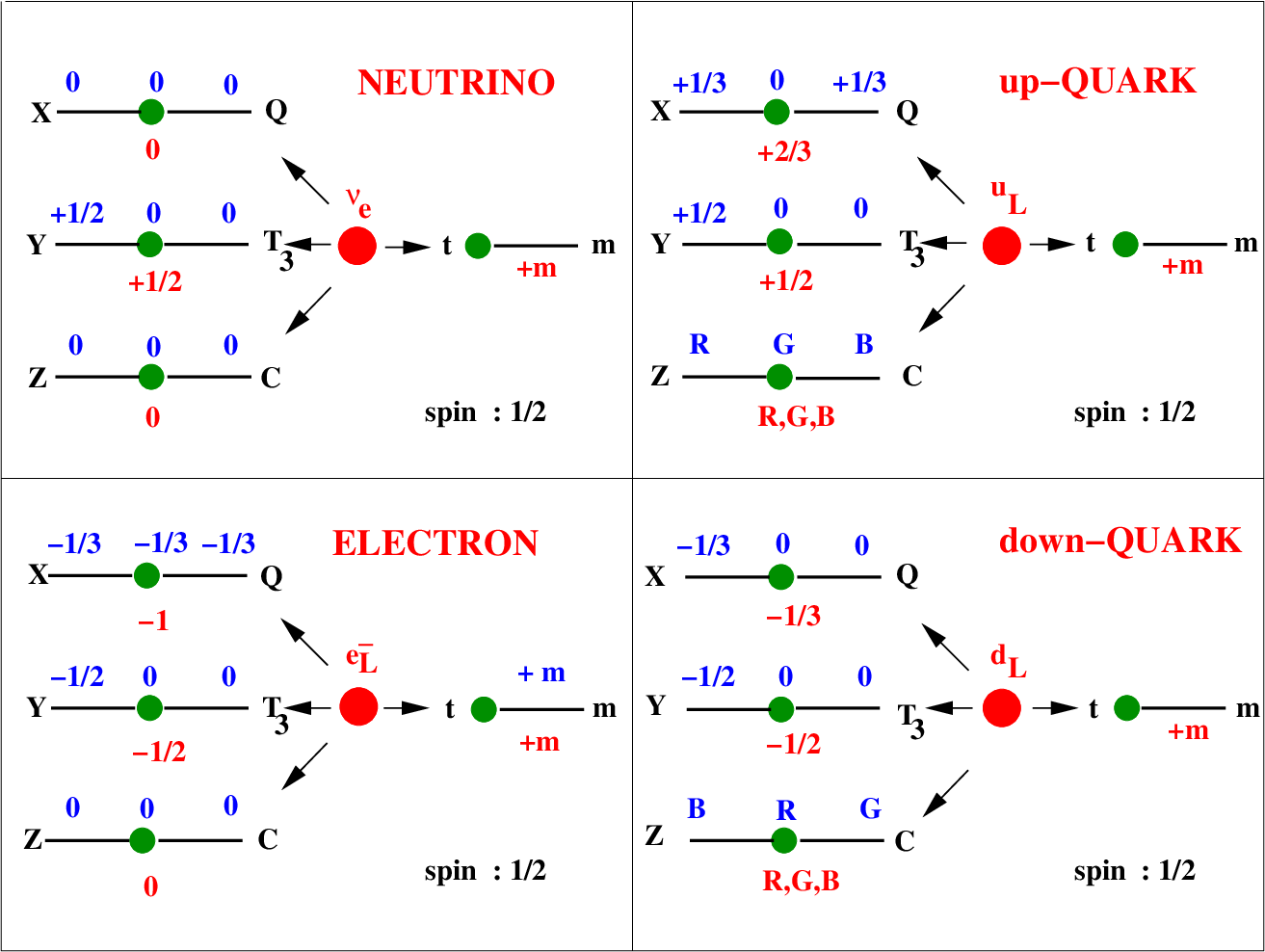
The experimental results for the electron neutrino are , the mass is [140] and . The spin is and the particle is left-handed. We choose for this reason all the electric charges zero in all possible positions above the x-axis and accordingly also the integral charge zero below the x-axis. A limit for the magnetic moment of [140] for the electron neutrino exist, what opens the possibility the carries electric charges. In this case the could be composed in a charge and an anti-charge placed above at two of the three free positions of the x - axis. The scheme would be still in agreement with the experiment because the integrated charge below the x-axis would be zero. For the weak charge three possible positions above the y-axis: left, center and right are open. If the would carry a weak moment it would be necessary to put the charge left or right above the y-axis. As this is not excluded so far we use the position y-axis left above. If the would carry no weak moment the charge must be placed in the center position above the y-axis. The total weak charge of the measured from far outside is also shown below the y-axis. The carries no color what sets the color charge above and below the z-axis. The experiments about life time and rest mass of the are not definite for the time being [140] we choose a non stable particle with rest mass below the t-axis.
The left handed electron we discussed just in very much detail in chapter 5.2.2 for this reason we repeat only the main points of these discussion. The particle carries three electric charges we placed on the three free position above the x-axis, the integrated charge is below the x-axis , placed left above the y-axis and the integrated charge is also placed below the y-axis and the color is zero consequently are all color above and below the z-axis zero. The particle has spin , with a mass of MeV and is very stable [137], for this reason is the mass assigned above and below the t-axis. The scheme request in agreement with the experiment [137] that the electron generates a magnetic moment, electric dipole moments and weak moments are possible.
The left-handed up-Quark is composed out of two anti charges which could be placed on two of the three free positions above the x-axis. The integrated charge is shown below the x-axis. All the possible positions of this two charges would to lead a magnetic moment of the . Similar like the for the , for the weak charge of the three possible positions above the y-axis left, center and right are open. If the would carry a weak moment it would be necessary to put the charge left or right above the y-axis. As this is not excluded so far we use the position y-axis left above [141]. If the would carry no weak moment the charge must be placed in the center position above the y-axis. The total weak charge of the measured from far outside is also shown below the y-axis. The color could be places above the z-axis in total 18 combinations ( , , , , , , , , , , , , , , , , and ). The color is assigned symbolic , , above the z-axis. The integrated total possible 18 charge combinations are shown symbolic below the z-axis. The color charges could generate color moments. The particle has spin , with a rest mass between MeV [138] and is stable only in a nucleus. We assigned it non stable with rest mass below the t-axis.
The left-handed down-Quark is composed out of one charges which could be placed at one of the three free positions above the x-axis. The choice of the position will generate on the mass kernel no magnetic moment and at the border a magnetic moment with opposite sign to the up-Quark . If the position of the two charges of the up-Quark is like in Fig.21 the magnetic moment of the up-Quark must be . Similar like for the , for the weak charge of the is . Three possible positions above the y-axis ( left, center and right ) are open. If the would carry a weak moment it would be necessary to put the charge left or right above the y-axis. Depending about further experiments [141] it would be possible to discover a weak moment or exclude it. In case of the exclusion the position of the weak charge must change accordingly to the center. The total weak charge of the measured from far outside is also shown below the y-axis. Like for the quark the color could be places above the z-axis in total 18 combinations ( , , , , , , , , , , , , , , , , and ). The color is assigned symbolic , , above the z-axis. The integrated total possible 18 charge combinations are shown symbolic below the z-axis. The color charges could generate color moments. The particle has spin , with a rest mass between MeV [138] and is stable only in a nucleus. We assigned it non stable with rest mass below the t-axis.
5.2.4 Scheme of the lightest right handed fundamental particles
In Fig.22 are displayed the scheme of all the right handed lightest FPs. The change from left handed FPs to right handed FPs is performed by the change of the weak charge from to . The rest of the quantum numbers stays the same. For this reason we discuss the scheme of the right handed FPs only brief.
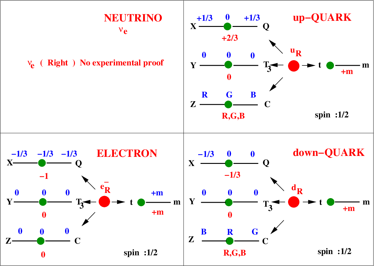
All experiments proofed that no right handed neutrino exist. For this reason is the scheme for the empty.
The right handed electron carries three electric charges we placed on the three free position above the x-axis, the integrated charge is shown below the x-axis. The weak charge and accordingly the integrated charge and the color is zero. For this reason are all weak and color charges above and below the y-axis and z-axis zero. The particle has spin , with a mass of MeV and is very stable [137] for this reason we assign the mass above and below the t-axis. The scheme request in agreement with the experiment [137] that the electron generates a magnetic moment, electric dipole are possible.
The right-handed up-Quark is composed out of two anti charges which could be placed on two of the three free positions above the x-axis. The integrated charge is shown below the x-axis. All the possible positions of this two charges would to lead a magnetic moment of the . The weak charge of the is . Accordingly we set all weak charges above and the integrated weak charge below the y-axis to zero. The color could be places above the z-axis in total 18 combinations ( , , , , , , , , , , , , , , , , and ). The color is assigned symbolic , , above the z-axis. The integrated total possible 18 charge combinations are shown symbolic below the z-axis. The color charges could generate color moments. The particle has spin , with a rest mass between MeV [138] and is stable only in a nucleus. We assigned it non stable with rest mass below the t-axis.
The right-handed down-Quark is composed out of one charges which could be placed at one of the three free positions above the x-axis. The choice of the position will generate on the mass kernel no magnetic moment and at the border a magnetic moment with opposite sign to the up-Quark . If the position of the two charges of the up-Quark is like in Fig.22 the magnetic moment of the up-Quark must be . The weak charge of the is . Accordingly we set all weak charges above and the integrated weak charge below the y-axis to zero. Like for the quark the color could be places above the z-axis in total 18 combinations ( , , , , , , , , , , , , , , , , and ). The color is assigned symbolic , , above the z-axis. The integrated total possible 18 charge combinations are shown symbolic below the z-axis. The color charges could generate color moments. The particle has spin , with a rest mass between MeV [138] and is stable only in a nucleus. We assigned it non stable with rest mass below the t-axis.
5.2.5 Scheme of the lightest right handed anti fundamental particles
In Fig.23 are displayed the scheme of all the right handed lightest anti-FPs.

The experimental results for the right handed anti electron neutrino are , the mass is small and . We place the electric charge above the x-axis to and the integral charge below also to . It is possible like for the left handed neutrino that the particle carries electric charges. In this case the could be composed in a charge and an anti-charge placed on two of the three free positions of the x - axis. The scheme would be still in agreement with the experiment because the integrated charge would be zero. The weak charge we place above the left side of the y-axis. As we have no experimental evidence of a weak moment is this a random decision. In this position the could generate a weak moment, the same would happen in the right position. The center position would generate a zero weak moment. The integrated weak charge below the y-axis is . The color charge above the z-axis is zero also the integrated color charge below the z-axis. The stability and mass of the particle is not experimentally not settled. We assume an unstable particle with a finite anti-rest mass and set the anti-mass below the t -axis. Experimental are the neutrino-antineutrino intrinsic properties not settled. It is not known is each neutrino mass eigenstate identical to its antiparticle or distinct from it, for we would have Majorana particles and for we would call it Dirac particles [87].
The right-handed positron is composed of three anti charges assigned above the x-axis and the integrated charge below x-axis. Similar to the left-handed electron it carries a weak charge but with positive sign . Three possible positions ( left, center and right ) are open. If the positron would carry a weak moment it would be necessary to put the charge left or right above the y-axis. As this is not excluded so far we use the position of he y-axis left above. The total weak charge measured from far outside the positron would be also shown below the y-axis. The positron carries no color what sets the color charge above and below the z-axis. The particle has spin , with a anti-mass of MeV and is very stable , for this reason is the mass assigned above and the anti-mass below the t-axis. The scheme request that the positron generates a magnetic moment like the electron an electric dipole moment is possible.
The right-handed anti-up-Quark is composed out of two charges which could be placed on two of the three free positions above the x-axis. The integrated charge is shown below the x-axis. All the possible positions of this two charges would to lead a magnetic moment of the . The weak charge of the . Three possible positions above the y-axis ( left, center and right ) are open. If the would carry a weak moment it would be necessary to put the charge left or right above the y-axis. As this is not excluded so far we use the position y-axis left above [141]. If the would carry no weak moment the charge must be placed in the center position above the y-axis. The total weak charge of the measured from far outside is also shown below the y-axis. The anti-color could be places above the z-axis in total 18 combinations ( , , , , , , , , , , , , , , , , and ). The anti-color is assigned symbolic , , above the z-axis. The integrated total possible 18 charge combinations are shown symbolic below the z-axis. For simplicity we use in Fig.23 for color and anti-color the same symbol. The anti-color charges could generate anti-color moments. The particle has spin , with an anti- rest mass between MeV [138]. We assigned it non stable with anti-rest mass below the t-axis.
The right-handed anti-down-Quark is composed out of one anti-charge which could be placed at one of the three free positions above the x-axis. The choice of the position will generate on the mass kernel no magnetic moment and at the border a magnetic moment with opposite sign to the anti-up Quark . If the position of the two charges of the anti-up-Quark is like in Fig.23 the magnetic moment of the anti-up Quark must be . Similar like for the , the weak charge of the is . Three possible positions above the y-axis ( left, center and right ) are open. If the would carry a weak moment it would be necessary to put the charge left or right above the y-axis. Depending about further experiments [141] it would be possible to discover a weak moment or exclude it. In case of the exclusion the position of the weak charge must change accordingly to the center. The total weak charge of the measured from far outside is also shown below the y-axis. Like for the quark the anti-color could be places above the z-axis in total 18 combinations ( , , , , , , , , , , , , , , , , and ). The anti-color is assigned symbolic , , above the z-axis. The integrated total possible 18 charge combinations are shown symbolic below the z-axis. For simplicity we use in Fig.23 for color and anti-color the same symbol. The anti-color charges could generate anti-color moments. The particle has spin , with an anti- rest mass between MeV [138]. We assigned it non stable with anti-rest mass below the t-axis.
5.2.6 Scheme of the lightest left handed anti fundamental particles
In Fig.24 are displayed the scheme of all the left handed lightest anti-FPs. The change from right handed anti-FPs to left-handed anti-FPs is performed by the change of the weak charge from to . The rest of the quantum numbers stays the same. For this reason we discuss the scheme of the right handed FPs only brief.

No experimental proof of a left handed anti-neutrino exist. For this reason is the scheme for the empty.
The left handed positron carries three electric anti-charges we placed on the three free position above the x-axis, the integrated charge is shown below the x-axis. The weak charge and accordingly the integrated charge and the color is zero. For this reason are all weak and color charges above and below the y-axis and z-axis zero. The particle has spin , with a mass of MeV and is very stable [137] for this reason we assigned the mass above the t-axis and with a finite anti-rest mass below the t-axis. The scheme request that the electron generates a magnetic moment an electric dipole would be possible.
The left-handed anti-up-Quark is composed out of two charges which could be placed on two of the three free positions above the x-axis. The integrated charge is shown below the x-axis. All the possible positions of this two charges would to lead a magnetic moment of the . The weak charge of the is . Accordingly we set all weak charges above and the integrated weak charge below the y-axis to zero. The anti-color could be places above the z-axis in total 18 combinations ( , , , , , , , , , , , , , , , , and ). The anti-color is assigned symbolic , , above the z-axis. The integrated total possible 18 charge combinations are shown symbolic below the z-axis. For simplicity we use in Fig.24 for color and anti-color the same symbol. The anti-color charges could generate anti-color moments. The particle has spin , with an anti- rest mass between MeV [138]. We assigned it non stable with anti-rest mass below the t-axis.
The left-handed anti-down-Quark is composed out of one anti-charges which could be placed at one of the three free positions above the x-axis. The choice of the position will generate on the mass kernel no magnetic moment and at the border a magnetic moment with opposite sign to the anti-up-Quark . If the position of the two charges of the anti-up-Quark is like in Fig.24 the magnetic moment of the anti-up-Quark must be . The weak charge of the is . Accordingly we set all weak charges above and the integrated weak charge below the y-axis to zero. Like for the quark the anti-color could be places above the z-axis in total 18 combinations ( , , , , , , , , , , , , , , , , and ). The anti-color is assigned symbolic , , above the z-axis. The integrated total possible 18 charge combinations are shown symbolic below the z-axis. For simplicity we use in Fig.24 for color and anti-color the same symbol. The anti-color charges could generate anti-color moments. The particle has spin , with an anti- rest mass between MeV [138]. We assigned it non stable with anti-rest mass below the t-axis.
5.2.7 Scheme of the gauge bosons
In the simplest structure of the SM two fundamental spin particles interacting with each other through spin point particles for the strong, electro magnetic and weak interaction as shown in Fig.2. If our scheme for geometrical extended fundamental particles introduced for example in Fig.17 is general valid for FPs it is important to test the scheme is also able to describe the the gluons, and .
Scheme of the eight gluons of the strong interaction
In the SM are eight gluons necessary for the strong interaction between the six quarks. All the gluons are combinations of colors and anti colors located at one single point. The gluons carry no electromagnetic or weak charge . Also the rest mass is zero but the carry induced mass of . In a scheme where the gluon is a geometrical extended object has this the consequence that the x-axis and y-axis is not populated. The object look from the point of view of the three charges of the SM like a string. Only the induced mass in the kernel will lead to an geometrical extension. To respect these experimental findings we populate only the z-axis in agreement with Fig.17 and do not show the x-axis and y-axis in the scheme. The t-axis we keep as before. We follow in Fig.25 this pattern and locate the nine possible color anti color combinations ( ) like for the fermions at three positions above the z-axis. The choice of the position left, center or right would depend about a color moment of the gluons. As no experimental evidence about such a moment exist we took a random choice. The eight integrated gluon combinations seen from far outside, the gluon ( ) are placed below the z-axis. The gluons carry only induced mass of we placed it below the t-axis. The spin of the gluons assigns on specific direction of the object, we choose in accordance with Fig.17 the z-axis. To locate the carrier of the color force color and anti-color in one location of the three geometrical axis is not the only possibility in the scheme under discussion. It would be possible to separate the color and anti-color at two geometrical separated positions. For the combination maximal six free positions would be necessary. These position would exist at the three axis x, y and z surrounding the porter of the mass kernel as shown for example in Fig.17. Such a configuration would generate a spherical closed structure but would need three coordinates. We follow in Fig.25 the assumption that every free space coordinate is acting like a free parameter for the three interactions strong, electromagnetic and weak and use only one axis the z-axis.

Scheme of the gauge bosons and
The most interesting particle is the , it carries no charges , no rest mass only induced mass or energy and . The spin assigns a distinct axis and polarization features as longitudinal or circular polarization. From experiment we know it is a wave or a particle depending about the experimental question we ask. It is his own anti- particle. An geometrical extension could be originated from a induced mass kernel surrounded by an charge and anti-charge or self interacting electromagnetic field. In the scheme shown in Fig.26 we set all charges above and below the three geometrical axis to zero. The induced mass or energy we place below the t-axis. Our scheme would define the as a poor time like object with an induced mass kernel.

The carrier of the weak interaction in the SM model are the weak bosons and . The is the partner of the with charges , with but with a rest mass of GeV [136]. It is his own anti-particle. A geometrical extension could be very similar as for the but the mass kernel would be generated by a high rest mass as displayed in Fig.26 below the t-axis in and . As for the are the charges , we set in Fig.26 all the charges above and below the three geometrical axis to zero.
The weak boson carries three electric charges , two weak charges no color charge and a rest mass of GeV [136]. In Fig.26 we place the three electric charges above the x-axis on the three free positions. The scheme request in accordance with the SM, that the carries a magnetic moment [142]. The integrated charge is shown below the x-axis. The two weak charges we put above the y-axis left and right. The integrated weak charge is placed below the y-axis. The weak bosons are the FPs with an integrated weak charge together with the fermions with an integrated weak charge and support this fact the assumption to cluster the weak charge in units of . This leads to the sequence of the weak charge already discussed in Fig.20 of . The geometrical position of the charge ( left,right ) will generate a weak moment what will be bigger as the moment generated by the position ( center,right ) or ( center,left ) like . As no experimental evidence of a weak moment of the exist we took a random choice about the position. The color charge above and below the z-axis we set to zero because the carries no color charge. The particle has with a rest mass we assigned below the t-axis.
The weak boson carries three electric anti-charges , two weak charges , no color charge and a rest mass of GeV [136]. In Fig.26 we place the three electric anti-charges above the x-axis on the three free positions. The scheme request in accordance with the SM, that the carries a magnetic moment with opposite sign to the moment [142]. The integrated anti-charge is shown below the x-axis. The two weak charges we put above the y-axis left and right. The integrated weak charge is placed below the y-axis. Similar like for the will the geometrical position of the charge ( left,right ) generate a weak moment what is bigger as the moment generated by the position ( center,right ) or ( center,left ) like . As no experimental evidence of a weak moment of the exist we took a random choice about the position. The color charge above and below the z-axis we set to zero because the carries no color charge. The particle has with a very similar rest mass like the it is GeV [136]. We assigned the anti-rest mass of the as below the t-axis.
5.2.8 Excited states of fermions
The discussed scheme for geometrical extended fundamental particles includes so far all lightest left and right handed FPs, lightest left and right handed anti-FPs of the first particle family and the gauge bosons. The majority of the FPs belong to the second and third family. To test the reliability of the scheme under discussion it is essential to proof is the scheme able to describe also the second and third family.
Coincidence between three space coordinates and three families.
It would be possible to include also these particles in the described scheme, but all these following scheme structures would be very similar like in Fig.21, Fig.22, Fig.23 and Fig.24. It is remarkable that the charges, position of charges and the left/right handed structure of the heavier FPs is inside the families the same. The leading parameter to characterize from the experiment the difference between the three families is the rest mass of the fermions. The rest mass from family one, two and three is exponential increasing with the family number and [137]. Concerning our ETAMFP model in Fig.17 is the mass of the geometrical extended FPs located in the center of the particle. It is for this reason sensible to search for a possibility how the mass sphere could increase its mass or energy. As the spin of all three particle families is the same a vibration of the mass sphere of the fermions would be a possibility to increase the rest mass or energy. The mass sphere has in accordance with the three Cartesian coordinates three basic degrees of freedom to vibrate. This fact coincide with the three fermion families. For example the and would be the excited states of the . A harmonic oscillator with the vibration energy ( neglecting the zero energy ) would allow to use the three space coordinates , and of our scheme to install at the x-axis , on the y-axis and on the z-axis vibration states. The ground state would be and , the first excited state and and the third excited state . The mass sphere of the FPs would fulfill a rotational movement superimposed be a vibration in three axis as shown in Fig.27. The oscillation is limited by the essential condition not to change the spin of the FPs.

In the center of Fig.27 the three vibration states are symbolized by three coordinate systems. The mass of the three families is displayed on top of z-axis of these coordinates. The spine is symbolized by a twisting arrow below the z-axis. The spin axis is chosen to be parallel the z-axis. The ground state on the x-axis is shown left, the first excited state on the y-axis in the middle and the second exited state on the z-axis on the right in Fig.27. The ground state on the x-axis would be a rotating spherical mass sphere with a distinct rotating axis parallel the spin symbolized as red circle in the x-y plane. The first excited state on the y-axis would be a rotating ellipsoid mass sphere around the z-axis and vibrating at the same time with his mean axis in x and y direction, symbolized by an red and green ellipsis in the x-y plane. The first excited state on the z-axis would be a rotating ellipsoid mass sphere around the z-axis and vibrating at the same time with his mean axis in x,y and z direction, symbolized by a red, green and black ellipsis in the x-y plane and x-z plane.
Empirical attempt to sort all three particle families in one scheme.
The discussed conditions open the possibility to sort all the masses of fermions in an empirical attempt of a rotator superimposed with a highly degenerated oscillator. Depending about the number of parameters and constant factors what will be used it is possible to calculate the masses of all fermions. Using 2 parameters and 7 constants for 12 fermion masses it is possible to reach a moderate agreement between calculation and experimental date [143]. We introduce an example with 2 parameters and 10 constants for 12 fermion masses which allows to calculate precise all masses of the fermion and anti-fermions including a prediction about the mass limits for the and neutrino in Eq.56.
| (56) | |||||
Eq.56 contains the two parameters family number and the electric charge of the fermions. For simplicity the weak charge and color charge is not used, but is implicit hidden in the 10 constants. The first parameter is the family number according Fig.27 with as fibration state for the x,y and z-axis. The first family is and which leads to . The second family is and which leads to . The third family is which leads to . More exited states are mathematical possible. Experimental evidence and limits are discussed in chap.2.2 and chap.2.3. The second parameter is the charge for the leptons/anti-leptons and quarks/anti-quarks. Included in Eq.56 are the 10 constant factors MeV, MeV, MeV and MeV to define the masses of the first family. The constant factors for the leptons/anti-leptons are and ,for the quark/anti-quark family the factors and and for the for the quark/anti-quark family the factors and .
Comparison of calculation and experimental data.
The comparison of calculation and experimental data is shown in Fig.28. The plot displays on the x-axis the family number and on the y-axis the rest mass of the fermions in MeV. The experimental data are shown in black rectangles. The calculation for the rest mass of the quark is displayed as black dotted line, for the quark displayed as black dot dashed line, for the leptons displayed as black dashed line and for the neutrinos displayed as black solid line.

The experimental data are taken from ref. [2]. For the quarks with the charge , , and , we used as data the geometrical middle value of the experimental mass limits from ref. [2]. The same middle values for the experimental rest mass we used for the quarks with the charge , and . For the charge leptons , and we used the well measured rest masses from ref.[2]. For the neutrinos exist mass limits only. For this reason we use the mass limit for the as start value and calculate the mass limits for the and ( black solid line). We assume for the calculation the same exponent as for the charged leptons. The experimental limits ( black rectangles ) are much higher as the calculation. Further experiments are necessary to proof is this a fact of the accuracy of the experiment or an effect of the calculation. The perfect agreement between experimental measured rest mass and calculation of Eq.56 for the quarks and leptons is obvious, because total 12 parameters allow to calculate 12 rest masses.
The mass increase for the first family from follows approximately the strength of the weak, electro magnetic and strong coupling constants of the three interactions. It is visible in Fig.28 that the gradient of the mass increase per family is very similar for the charged leptons and the quarks with charge . The quarks with charge in particular the mass of the quark does not follow this trend. The upper experimental mass limit for the quark with 4 MeV just touches the lower mass limit of the quark with also 4 MeV. With improved experimental date in the next years this disagreement will may be disappear.
5.2.9 Conclusion about the scheme of geometrical extended fundamental particles and anti-particles
In conclusion it was possible to demonstrate, the hypotheses, the time and size development of the history of the very young universe forms the geometrical extension of the FPs, allows to sort all FPs in a common scheme. The mass increase for the first family follows approximately the strength of the weak, electro magnetic and strong coupling constants of the three interactions. The scheme predict a general similar tendency of the gradient of the mass increase per family for the leptons and quarks. The scheme shows that the link between geometrical space and time is of essential importance. Four interactions coincide with the four coordinates of our universe. The three families are in this philosophy the possibility of the mass kernel to oscillate ( link time ) in these three space coordinates. The scheme also shows the most simple charged highly symmetrical geometrical object is the electron. It serves as ground state for all leptons with a extremely high stability.
5.3 Classical approach to estimate the size of an electron determined from its experimental measured parameters
In the discussed scheme in Fig.17, Fig.20 and Fig.21 is the electron the most fundamental particle. It has a spherical geometrical structure, is the ground state of the leptons and is very stable with a life time of yr. It is for this reason a very important object to study the consequences of the rest mass, charge, spin, magnetic and possible electric dipole in accordance with our particle scheme of a geometrical extended object. Inspecting our basic scheme of an geometrical extended FP in Fig.17 the mass center and the charges and will fulfill a rotation orbiting the coordinate center . Immediately three questions concerning about a classical approach are coming up. Is the size of the electron bigger as the Planck size of cm ? Latest at the Planck scale gravity must be quantized and a classical picture would get meaningless. Does a scenario about the forces in the electron exist to form such a stable object? Why are the accelerated charges and are not emitting energy in form of radiation for example light?
The experimental limits about the size of fermion shown in Fig.10 are cm and for the electric dipole moment e cm. These limits are fare above the Planck Scale. The difference is with respectively magnitudes so far away from the Planck scale that we believe a classical approach has still some meaning.
In the chapter forces and stability ( chap.5.1.4 ) we discussed a possible scenario in Fig.18 and Fig.19 how such a stable object schematically could exist. In case of the electron point in Fig.18 would be the not rotating inner mass kernel, the rotating mass center would extent to point on where the charges and would be placed. This scenario would assume at the radius the mass density goes to zero and the radius where the charges are placed are about the same . The same stability scenario also explains that two electric charges are place opposite to each other on the x-axis shown in Fig.21 and one charge at . As consequence the magnetic moment and possible electric dipole moment of the electron get only generated from a total charge and not . For simplicity of the further discussion we will neglect the weak charge .
The extreme high experimental proved stability of the electron ask for a radiation free path of the charges around the center of the electron. This experimental fact request the charges do not undergo any acceleration because charge rotating on a circle is accelerated. In the chapter about a flashing vacuum ( chap. 5.1.5 ) we discussed a microscopic scenario about such a radiation free path. In this picture the vacuum has the important property to move a charge geometrical over a certain curvaceous path without acceleration. In this manner the curvaceous path for a charge get radiation free. An important consequence of such a type of path is that the geometrical length of the path will be contracted by the Lorentz transformation if the velocity of the charges approach the speed of light.
For the following calculations we need a numerical basis about the parameter mass, charge, spin, magnetic and possible electric dipole moment of the electron together with the Planck Constant, speed of light and Bohr Magneton. These parameters are summarized in Tab. 14 and taken from ref.[137].
| parameter | Symbol | value |
|---|---|---|
| Total Mass | MeV | |
| Charge | A s | |
| Weak Charge | ||
| Spin | MeV s | |
| Magnetic Moment | ||
| Electric Dipole Moment | e cm | |
| Planck Constant | MeV s | |
| Speed of Light | m/s | |
| Bohr Magneton | MeV/T |
In Tab. 14 the electron charges are the source of a electric, weak and gravitational force and should be able to polarize and curve the vacuum in the finiteness of the mass core. Following Einstein equation in Tab. 12 the mass of the electron would be originated from these curvatures. The spin of an geometrical extended electron is classically described by a gyroscope with a defined spin axis and a moment of inertia. The spin axis is perpendicular to a surface of rotation. The same counts for the classical magnetic moment of a charge. The charge rotates in our scheme like a point around the mass core of the object. As we know from experiment that the axis of the spin is anti-parallel to the axis of the magnetic moment it is likely that the charge rotates in the same surface of rotation as the mass core. If the charge in Fig.17 is considered as point it must cause an electric dipole moment if an spectator measures the dipole moment in the x-y plane and the electron is polarized parallel to the z-axis. The degree of polarization and the conditions of the experimental apparatus will affect the measured value of the dipole moment. The experiment is extreme difficile and is not settled so far.
In the following sections in this chapter we study with an increasing refinement of the classical electron model the impact of the different parameters of the electron on the size of the electron.
5.3.1 Mass and charge radius of an electron as gyroscope
To study the order of magnitude in a first simple approach we describe the microscopic structure of the electron as a rotating sphere like a gyroscope filled with mass as shown in Fig.17. The charges, spin and spin axis are in accordance also with Fig.17. In our scheme the electron as ground state of the leptons carries no fibration energy. The total energy of a gyroscope is under this conditions the sum of the energy of the electron and the rotational energy of the gyroscope as displayed in Eq.57.
| (57) |
The angular momentum is shown in Eq.58
| (58) |
and the magnetic moment of the electron in Eq.59.
| (59) |
is the moment of inertia of the mass core, and the angular velocity of the mass core and the charge and the radius the point like charge is located from the center.
The intention of this first approach is to study only the order of magnitude of the size of the electron. For this reason we calculate possible limits on the angular velocity from the experimental values. A lower limit for can be deduced from Eq.58 which allows a small but not zero for . An upper limit for can be calculated if we set in Eq.57 the rest mass . Inserting Eq.57 in Eq.58 and set it is possible to calculate with values from Tab. 14 the angular velocity in Eq.60
| (60) |
As discussed it is known from the experiment that the plane of rotation from the charge and the mass of the electron is the same no experimental information exist about the angular velocity and of the mass and charge. It is also not known in which distance from the center the mass density goes to zero and on which radius the point-like charge is located. If we follow our discussion about forces and stability in the introduction of this chapter it is likely to assume between and a certain functional interaction like exist.
For a working hypothesis we follow this philosophy to use first the simplest possible assumptions set and . Both hypotheses are supported by the discussion in chapter the pseudo charge of the gravitational interaction ( chap. 5.2.1 ), because the mass of the electron will be with high likelihood generated by the electric charge of the electron. This charge is mostly located after our ETAMFP model at the radius and the charge is rotating around the center what supports the assumption that the angular velocity of the charge and mass is the same. Using Eq.59, the angular velocity and for simplicity set the charge it is possible to calculate with the radius in Eq.61 and with Eq.60 in Eq.62.
| (61) |
| (62) |
The in this simple approach estimated limits for the radius are very huge. In particular the radius is totally in conflict with our experimental data discussed for example in Fig.10. We will for this reason ignore this limit for the further discussion. For the guidance of the next approach more interesting is the limit for .
The radius is fare away from the Planck or Grand unification scale , what supports our assumption to use for this calculations a classical ansatz. The velocity of the outer mass radius and the charge ( ) is bigger as the velocity of light .
To include this fact for the next approach it would be possible to use the special relativity or the general relativity. We discussed already the charge of the electron orbits on a radiation free path. This is the same condition as the charge would move with constant velocity along a straight-line. We use for this reason in the following section the special relativity in form of the Lorentz transformations to avoid velocities .
5.3.2 Charge radius of electron as Lorentz contracted gyroscope
To study the next order of magnitude in a second approach we describe the microscopic structure of the electron as before as rotating sphere like a gyroscope filled with mass as shown in Fig.17. The charges, spin and spin axis are in accordance also with Fig.17. We keep the condition of the radius . But we include in this approach the result of the last calculation and take into account the velocity of the outer mass radius and the charge is bigger as the velocity of light and we include the mass .
We just discussed the radiation free path length of the mass radius and charge must be corrected be the special relativity. It is necessary for this correction to distinguish between the radius an observer placed on the rotating system will measure and the radius an observer far away in rest will measure. This implements the observer in rest from fare outside the electron will measure a Lorentz contracted if the velocity of the charge approaches . The charge is not sensitive to the special relativity and the angular velocity is visible only for an observer in rest. The moving charge does not behave like a clock on the plane of rotation. For this reason exist only the angular velocity . The measured magnetic moment is originated from a charge moving along the path what is really contracted in this rotating system is the radius shown in Eq.63.
| (63) |
Lorentz contraction affects magnetic and electric dipole moment of electron
Using the data from Tab. 14 for the magnetic and the electric dipolmoment of the electron it is remarkable the is a finite well measured number and is very small in the frame of the error still zero. Our just discussed simple approach points in a direction the speed of the charge is close to the speed of light. Concerning the Lorentz contraction of the radius in Eq.63 to the question rises which radius or together with the charge is generating the magnetic and electric dipolmoment of the electron measured from an observer in rest in the laboratory. In other words to which radius or is the experiment sensitive to measure or . We study for this reason the limits for and given from the experimental values and our ETAMFP model to use or .
To set a limit on for the case generates the magnetic moment of the electron measured from an outside observer in rest, we assume after the discussion above the most likely case . The radius get contracted from Eq.63 to . The magnetic moment reads under this circumstances like in Eq.64.
| (64) |
The velocity of the charge is displayed in Eq.65
| (65) |
Replacing in Eq.64 with Eq.65 allows to calculate the discussed limit in Eq.66 if we insert the numerical values from , from Tab. 14 and from Eq.60.
| (66) |
This limit is close to the experimental measured value shown in Eq.67.
| (67) |
To set a limit on for the case generates the magnetic moment of the electron measured from an outside observer in rest, we assume after the discussion above again the most likely case . The radius in the rotating system will be finite and contracted by equation Eq.63 to . The angular velocity will by finite. The limit is zero as shown in Eq.68.
| (68) |
This limit is absolute in disagreement with the experimental measured value shown in Eq.69.
| (69) |
To set a limit on for the case generates the electric dipole moment of the electron measured from an outside observer in rest, we assume again the most likely case . The radius get contracted from Eq.63 to . The electric dipole moment reads under this circumstances like in Eq.70 if we replace by using Eq.63.
| (70) |
Replacing in Eq.70 with Eq.65 leads to the limit for in Eq.71 if we use again from Tab. 14 and from Eq.60.
| (71) |
This limit is about 17 magnitudes away from the experimental measured value shown in Eq.72.
| (72) |
To set a limit on for the case generates the electric dipole moment of the electron measured from an outside observer in rest, we assume again the most likely case . The radius in the rotating system will be finite and contracted by equation Eq.63 to . The angular velocity will by finite. The limit is zero as shown in Eq.73
| (73) |
This limit is approximately in agreement with the experimental measured limit shown in Eq.74.
| (74) |
Inspecting the just discussed limits, the answer from the comparison between the experimental values and the calculated limits for the magnetic and electric dipole moment of the electron concerning which radius or has to be used from the Lorentz contraction is rather clear. The measurement of the magnetic moment of the electron is sensitive to the radius . This is the radius an observer located in the center of the electron would measure from the center to the charge if he rotates with . The measurement of the electric dipole moment is sensitive to the Lorentz contracted radius an observer will measure if he is located fare outside the electron in rest. In this sense the Lorentz contraction in our discussed model Fig.17 would explain why the magnetic moment is a finite well measured number and is very small in the frame of the error still zero.
Limits of the parameters of the electron after Lorentz contraction.
Our approach about an geometrical extended electron is at this stage so far developed to estimate the parameters , rest mass , rotational energy , and under the condition the speed of the rotating charge is close to the speed of light . Further following this stage the magnetic moment of the electron is described by the Eq.64 and the angular velocity from Eq.65 where and is depending about .
| (75) |
| (76) |
We assumed as in the first approach the angular velocity of the mass center and the charge is the same . This allows to write down together with Eq.58 the rotational energy in the form of Eq.77
| (77) |
| (78) |
| (79) |
If we set and take for the charge , the speed of light and the magnetic moment the numerical values from Tab. 14 is is possible to calculate . We calculated for the discussed option is generated from a total charge as discussed for our ETAMFP model in Fig.17 and for the possibility this charge is . The numerical values are calculated with Eq.75 and shown together with the assumption in Tab. 15 first three lines. If the angular velocity is known for the case the charge responsible for is or it is possible to calculate with Eq.78 the rest mass for both options and displayed in Tab. 15 in the fourth and fifth line. For the same both options it is possible to calculate with Eq.77 the rotational energy and taking into account and and the total energy with from Tab. 14. The numerical values are shown in Tab. 15 in the sixth and seventh line. Also for both options it is possible to calculate with Eq.79 the radius and taking into account and and the from Tab. 14 including . The numerical values are shown in Tab. 15 in the eighth and ninth line. In the last line of Tab. 15 the numerical value for the Lorentz contracted radius is shown. This value must be of course close to zero.
| parameter | Symbol | value |
|---|---|---|
| velocity charge | ||
| angular velocity | 1/s | |
| angular velocity | 1/s | |
| rest mass | MeV | |
| rest mass | MeV | |
| rotational energy | MeV | |
| rotational energy | MeV | |
| charge radius | m | |
| charge radius | m | |
| charge radius rest system | m |
The status of the just discussed estimation of this approach is the speed of the rotating charge is close to the speed of light . Including the Lorentz contraction of the charge circling the center of the electron it explains why the magnetic moment is rather big and the electric dipole moment very small. Certainly after the discussion about the scale dependence of the SM and BBM the radius will be not zero. It is also not possible in this approach to distinguish between the and for the calculated parameters , , and .
5.3.3 Mass and charge radius of electron as Lorentz contracted gyroscope
So far our discussed model did not include a specific assumption about the mass core of the electron. In the discussion about the geometrical approach of the FPs summarized in Fig.17 we assumed the mass of the of the FPs contains two parts. An inner non rotating mass kernel, the seeds of a quantized energy mass condensate of the Planck Era and a rotating mass density distribution the seeds of the mass between Planck and GUT Era. In the chapter about exited states of fermions ( chap.5.2.8 ) we discussed in Fig.28 the possibility to describe the electron as the vibration ground state of the leptons. An energetic favorable object of such a mass core would be a classical rotating sphere like a gyroscope with a rotating axis as spin axis.
Mass core as Lorentz contracted rigid sphere
Following the philosophy to use a simple as possible approach the most easily accessible assumption is to use a rigid sphere, with constant mass density, circling the spin axis with the angular velocity and a border at radius . The mass moment of inertia is in Eq.80 a function of the mass and the radius .
| (80) |
The according rotational energy is displayed in Eq.81
| (81) |
We assumed in Eq.80 the radius where the mass density ends coincides like in Fig.17 with the radius where the charge is located . If we assume again like in the previous chapter about the charge radius, the speed of the surface of the mass sphere at the position perpendicular to the spin axis will exceed the speed of light. The conditions will be very similar as in the case of the charge. In accordance to our discussion in chap.5.1.5 we assume the mass and the radius in Eq.80 have to be corrected with the Lorentz transformations. In our simple model of a rigid sphere will only be the mass ring with a half moon shaped cross section in the vicinity of sensitive to . The mass content of this ring decreases fast to zero if the inner radius of this ring approaches . This mass decrease is damping the increasing sensitivity to , if is approaching at . In contrast is the mass less surface ring of the sphere in the vicinity of fully exposed to the sensitivity to and will be substantial contracted because will be very close to . In the limit of the surface ring will be in the vicinity of contracted to a point in the center of the sphere.
To apply the Lorentz transformations on Eq.80 we first estimate the magnitude of the sensitivity of and to .
We begin with the sensitivity of . The mass distribution of a rotating sphere is shown in Fig.29. On the left side in Fig.29 is drawn the mass sphere in two dimensions ( z-axis and x-axis ) rotating parallel with the spin to the z-axis. On the right side middle upper part is displayed the mass distribution of the sphere in arbitrary units as function of the of for a constant mass density. The mass distribution ( solid black line ) decreases from 100 [au] at to zero at . The graph below on the right side of Fig.29 shows the linear increase if as function of according Eq.65. The graph total right side in Fig.29 displays the Lorentz factor as function of as black solid line. If we fold the , and dependence from it is possible to calculate the correction for the mass . The correction at , increases to a maximum at approximately and approaches at or . This is displayed in the mass plot middle upper part ( red broken line ) of Fig.29. Comparing the black line with the red broken line in this plot it is visible that the Lorentz correction is active only for shown in the black hatched half moon shaped area of Fig.29 left side. The total mass increase originated by the Lorentz transformation is approximately if at . We used so far in this simple model a constant mass density distribution from to . Following the discussion in chap. 5.1.2 and Fig.17 we expect a mass distribution which deceases from to sharply to in the vicinity of . This will suppress the above discussed edge effect of the rotating sphere to be negligible at . We ignore for this reason the Lorentz correction of in the following calculations.

Second we estimate the dependence of . The border of the rotating sphere is a mass less shell rotating at with maximal . The surface velocity decreases if the distance from the spin axis get smaller and finally will be at the spin axis as shown in the lower plot on the middle side ( black solid line ) in Fig.29. The distance from the spin axis in the rotating system will undergo a Lorentz contraction of Eq.82 to the distance measured from an experiment outside the electron.
| (82) |
The application of Eq.82 on in arbitrary units is displayed in the plot total right side of Fig.29 ( red broken line ). The contraction put for at to zero and the radius at get not affected. A quarter of this contracted infinite thin shell is shown in the red broken line of Fig.29 left side. By inspection of Fig.29 it is obvious, the dependence of must by included to calculate the moment of inertia in Eq.80.
Model factor respecting not rotating inner mass kernel
After the discussion about the basic scheme in Fig.17 we expect not the whole mass of the electron rotates. This would imply the inner Planck Kernel does not contribute to the rotational energy. To respect this possible mass kernel we introduce a model factor . We expect this factor is because the decreasing influence of the inner non rotating mass kernel dominates the maximum possible increase of the mass at border of the mass sphere we investigated in the preceding paragraph. We modify for this reason the rest mass to model rest mass .
The experimental accessible radius from the electron discussed in chap.2.2 is sensitive in reaction to the mass radius of the electron and the radius the charges are loaded. The radius limit deduced of the electric dipolmoment of the electron is sensitive only to the radius the charges are loaded. We assume the charge of the electron is placed at the radius . The limits for this radius we discussed in Eq.73 and Eq.74. Following this discussion and Eq.82 we set at the minimal possible radius . If we collect our assumption about the different angular velocities, radius and model factor we end at , and . Including these assumptions we replace in Eq.80 the radius by the Eq.83.
| (83) |
Inserting the model factor and Eq.83 in Eq.80 we get the Lorentz corrected mass moment of inertia including all our assumptions in in Eq.84.
| (84) |
At this stage of the development of our ETAMFP model we investigate the impact of the so far introduced assumptions, about the mass and charge radius of a electron considered as Lorentz contracted gyroscope, on the model. We develop for this reason in a first step equations for the velocity , the angular velocity , the energy of and , the radius the Lorentz contracted radius as function of the model factor . In a second step we study the from the numerical measured parameters in Tab. 14 of the electron given numerical limits for the model factor in five plots , , , and .
Equations including model factor for rotating mass core
If we insert Eq.65 in Eq.84 and use Eq.81 it is possible to calculate as function from and in Eq.85.
| (85) |
Next we replace in Eq.64 with ( With as anomal magnetic moment ), use from Eq.65 and find Eq.86 the angular velocity as function of .
| (86) |
The experimental measured parameters , , , and are known and shown in Tab. 14.
Inserting Eq.86 in Eq.85 and using Eq.81 with the definition of we find the angular velocity as function of in Eq.87.
| (87) |
According our chapter of the schemes of fermions we use in Eq.87 the model depending charge where could be or .
To find a similar expression for we insert from Eq.78 in Eq.85 and replacing with Eq.87. This allows to calculate the velocity in Eq.88.
| (88) |
This equation depends only from the anomal magnetic moment , the reduced charge and the model factor .
A certain values of the model parameter defines via Eq.88 and Eq.87 a velocity and the angular velocity . Inserting for the calculation of the energy and we use Eq.78 and Eq.81. For the calculation of the radius we insert and in Eq.79.
For the last missing parameter we use Eq.65 resolved after and insert the angular velocity from Eq.87 and the velocity from Eq.88 to calculate Eq.89
| (89) |
The status of our calculations permits now to calculate the velocity , the angular velocity , the energy of and , the radius the Lorentz contracted radius as function of the model factor .
Numerical limits for model factor set by experiment
As announced in a second step we study the from the numerical measured parameters in Tab. 14 of the electron dictated numerical limits for the model factor in five plots , , , and .
Important for the whole following discussions is the test which charge or is in agreement with our so far discussed model. In Tab. 15 it was not possible to distinguish between the two possibilities.
If we insert and in Eq.88 we calculate an negative which will result in an imaginary . If we use the physical allowed limits for and we find the according limit for the model factor is ranging from . The imaginary for is in disagreement with the Lorentz transformation. The model factor ranging from is in disagreement with our expectation of .
If we insert in and in Eq.88 we calculate a slightly bigger as one of . Inserting in Eq.88 the physical allowed limits of and we calculate a model factor ranging from . It is interesting to notice that the anomal magnetic moment A and are the leading parameters in Eq.88 to decide about the numerical value of . According our ETAMFP model we expect a real and a model factor . This is in agreement with our geometrical approach of Fig.17 and the whole scheme of fermions where we assume the charge for the electron is placed in units at three possible locations. For this reasons we will in the following discussion only consider the case.
To calculate the plot we use Eq.88 and calculate the the model factor in the limit of .
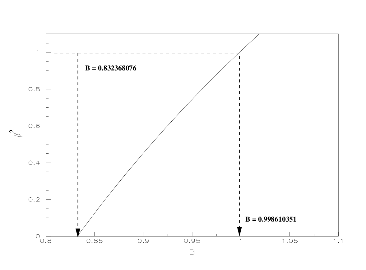
The solid black line in Fig.30 displays the discussed function. We find for the upper limit for and for a not rotating sphere accordingly a lower limit for shown in broken solid lines with arrow in Fig.30. The limits of are used in the following plots , , and to study the behavior of , and in the frame of our ETAMFP model.
To calculate the plot we use Eq.87 and vary from to to display in Fig.31 the whole possible range of . The solid convoluted black line in Fig.31 displays the discussed function.
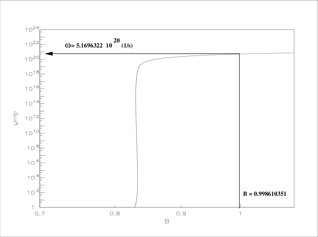
If we insert in Eq.87 which is in accordance with we calculate a maximum value of angular velocity . This value is in agreement with the value in Tab. 15 for and shown in Fig.31 as solid straight black line with arrow. If we insert in Eq.87 which is in accordance with we calculate of course a minimum value of angular velocity of important only for the completeness of the plot. A similar result we find if we insert in Eq.87 we find the maximum possible . This value is only of mathematical interest because it would exceed .
To calculate the plot and we vary the model parameter from to . Next we calculate with Eq.87 the according angular velocity and subsequent inserting in Eq.78 to get and Eq.81 to find . The black broken line in Fig.32 displays and the black solid line .

The maximum possible share for between and ist MeV or and MeV or . These values are in agreement with the numbers for and in Tab. 15 and marked by a blue dot dashed line with arrow on the right side in Fig.32. The lower limit for results in MeV and and is marked as blue dot dashed line with arrow at the left side in Fig.32 together with the numerical value for as dotted red line.
To calculate the plot we vary the model parameter from to , calculate with Eq.88 velocity with Eq.87 the angular velocity and insert these values in Eq.79 to find shown as black solid line in Fig.33.

An observer located in the middle point of the electron rotating with would measure a minimum possible allowed by the experimental date of for the condition and . This value is in agreement with the value for in Tab. 15 and marked by the crossing of the red dotted line with the blue dashed dotted line on the right side in Fig.33. The maximum of this radius will increase with decreasing slowly to at shown from the blue dashed dotted line left side in Fig.33. This singularity is certain not supported by the data because the electron has a finite spin, is only a mathematical option.
To calculate the plot for the Lorentz contracted radius of the electron measured from an observer outside the electron we vary the model parameter from to in Eq.89 and plot the black solid line in Fig.34.
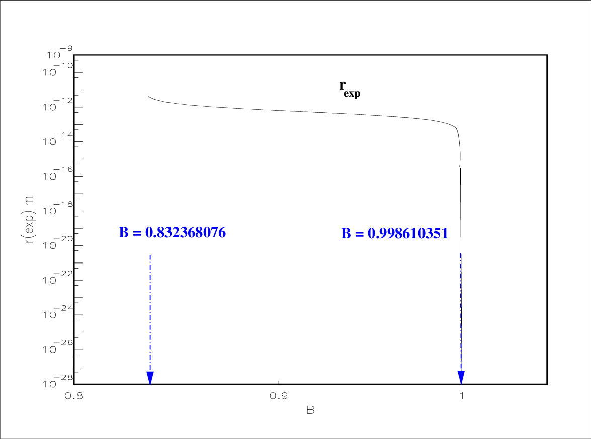
The square root structure of Eq.89 leads to a steep gradient singularity if what includes that also . This is shown by a blue dot dashed line with arrow in the right side of Fig.34. For reaches a maximum marked by a blue dashed dotted line with arrow left side in Fig.34. The possible from the experiment and model allowed values ranging from is .
5.3.4 Implication of the electric dipole moment of the electron on its geometrical extension
In all calculations so far we did not use the electric dipole moment of the electron because the experimental value is very small. The excellent , very important and ambitious experiments [22] measured so far for a value ( See for example shown in Tab. 14 ) comparable with zero, what has to be considered as a limit.
In all our considerations of the classical approach the charges of the electron ( For example in Fig.17 ) are separated by a distance . A classical dipole is constructed from two electric charges of different sign separated by a distance . Our ETAMFP model contains two electric charges from the same sign separated by a distance . In this sense is our model not a classical dipole but certainly very similar. Our considerations about the sensitivity of the experiment to measure the electric dipole moment in Eq.72 to Eq.74 come to the conclusion that the experiments measure the distance between the charges in the LAB-system. If we inspect the value for in Tab. 15 and the function of in Fig.34 it is obvious, if the speed of the charges approach the Lorentz contraction will push the radius against zero. This is in agreement with the minute measurement of . But the limit is still seven magnitudes away from the Planck scale, which is still a save distance to the quantization of the mass. We identify for these reasons with the measured electric dipole moment . In this sense is a direct measurement of the distance between the two charges circulating around the mass kernel of the electron measured from an observer outside the electron in the LAB-system.
Respecting the experimental challenge that a discovery potential of about for the measurement of the electric dipole moment of the electron is not reached so far and take into account the just discussed conditions, we introduce the dipole moment in our ETAMFP model and use the for the dipole moment deduced radius . In a first stage we take the from the observer in the LAB-system measured radius to calculate , the angular velocity , rest mass , rotational energy , the radius of the of the electron without any specific assumption about the mass kernel of the electron. It means we ignore the above discussed model factor . In a second stage we include this model factor .
For the first stage we calculate the radius from the electric dipole moment. As displayed in Fig.17 and Fig.20 the three charges are generating in our scheme the electric dipole moment. It would be possible to group the two outer charges or the inner charge two times with the outer charges what leads to the same result of the dipole moment shown in Eq.90.
| (90) |
The numerical value is taken from Tab. 14. The according experimental measured radius is given in Eq.91.
| (91) |
| (92) |
| (93) |
The equation for the speed of the charge of the electron we express in the very compact form of in Eq.94.
| (94) |
As the quadratic form of the value of is between . To calculate the angular velocity of the charges we resolving Eq.65 after and insert the K factor from Eq.93 in this equation what is shown in Eq.95.
| (95) |
| (96) |
| (97) |
Inserting Eq.94 in Eq.83 allows to calculate the charge radius of the electron in the rotating system in Eq.98.
| (98) |
We dispense to recalculate the different parameters of Tab. 15, with Eq.90 to Eq.98 because the change of the parameters is negligible if we assume .
As announced before in a second stage we include the model factor in our calculations. We first calculate the factor themselves as function of the magnetic moment , velocity of light , charge and radius summarized in the factor of Eq.93. Using Eq.94 and Eq.88 it is possible to calculate the model factor in Eq.99
| (99) |
The factor is written in the simple form as function of , the anomal magnetic moment and the reduced charge . Inserting the factor in they equations from Eq.85 to Eq.89 it is possible to study the influence of the electric dipole moment of the electron on our Lorentz contracted mass core.
It is for the further discussion of our ETAMFP model important to study the numerical impact of the measured value of the electric dipole moment on our ETAMFP model. We inserting for this reason the electric dipole moment from Tab. 14 in Eq.90 to Eq.98 to calculate the numerical values of the parameters , the angular velocity , rest mass , rotational energy and the radius of the . The numerical value are shown in Tab. 16.
| parameter | Symbol | value |
|---|---|---|
| velocity charge | ||
| angular velocity | 1/s | |
| rest mass | MeV | |
| rotational energy | MeV | |
| charge radius | m | |
| charge radius rest system | m | |
| model factor |
The first line in Tab. 16 displays the numerical value of the speed of the outer charges in form of calculated with Eq.94. This speed get pushed from the very small value of the electric dipole moment extreme close to . But the numerical value is not one. Inspecting Eq.94 it is obvious must be smaller as one depending about the numerical value of the factor of Eq.93 which is as always positive. The factor is a function of the magnetic dipole moment , speed of light , charge and the contracted radius derived from the electric dipole moment of the electron. The numerical extreme small measured value of the electric dipole moment pushes to a very high number shown Tab. 17 in the first line. As consequence calculated from Eq.94 is very close to one as displayed in Tab. 17 second line.
| parameter | value |
|---|---|
| K | |
| 0.99999999999999999999999999999999983608206299476884 | |
| B | 0.99861035118674254715174743056685316037852026506779 |
The second line in Tab. 16 displays the angular velocity the whole electron considered as a gyroscope circuits around an axis which coincides with the spin axis of the electron. The numerical values are the same as discussed in Tab. 15 for the case , what is after the just discussed high value a logical consequence.
The third line in Tab. 16 shows the rest mass of the electron calculated with Eq.96. Also this numerical value agrees with the numbers in Tab. 15 for the case .
The fourth line in Tab. 16 displays the rotational energy of the electron calculated with Eq.97. The numerical value agrees with the numbers in Tab. 15 for the case .
The fifth line in Tab. 16 displays the uncontracted radius of the mass boundary of the electron which coincides with the radius where the charges in Fig.17 are located calculated with Eq.98. This radius an observer would measure if he is placed in the center of the electron rotating with . The numerical value agrees with the Tab. 15 for the case .
The sixth line in Tab. 16 displays the contracted radius of the mass boundary of the electron. This coincides with the radius where the charges in Fig.17 are located. This radius an observer would measure if he is placed in in the LAB-system outside the electron in rest. The numerical values are taken from Eq.91 or recalculated for test of the high precision numeric as function of and as shown in Tab. 16.
Finally we calculated with Eq.99 the numerical value of the model factor which is shown in Tab. 16 last line. Numerical is this factor in Tab. 16 in agreement with the factor used in Fig.30 Fig.34 for the upper limit of for up to very high precision as shown in Tab. 17 in the last line. The measurement of the electric dipole moment of the electron locates the solution for , , the energies , , the radius and as function of displayed in in Fig.30 to Fig.34 as function of at the upper limit close to as shown in Tab. 17.
5.3.5 Estimation of the size of the mass kernel of the electron
After we introduced a model factor in the calculation of the rotating mass of the electron the calculation shows that the factor taken from Tab. 16 is , this is less as one. We conclude from this fact that the electron contains a non rotating mass kernel what would be a heritage of the Planck scale as discussed in Fig.16. If the density of the electron mass kernel and the density of the mass shell of the electron would be known and we use the simple relation of Eq.100
| (100) |
it is possible to write down a relation for the radius of the mass kernel of the electron for our ETAMFP like Eq.101.
| (101) |
If we recall the discussion in chap.5.1 it is only possible in the ETAMFP model to predict a general tendency about and . But if we follow the in Fig.16 discussed heritage ansatz it is possible to estimate the order of magnitude of .
To estimate the numerical magnitude of the radius we assume the ratio of the density at the GUT scale to the total mass density of the electron is the same as the ratio of the density of the Planck scale to the mass kernel of the electron . The density of the mass kernel reads than like Eq.102.
| (102) |
The density of depents about like Eq.103.
| (103) |
For the size of the GUT scale exist only approximate numbers. The current values in the literature are varying in a big range as shown in Eq.104 [149].
| (104) |
Implementing five different GUT scales in the range of Eq.104 in Eq.103 allows to calculate the according GUT densities . For and we used the values from Tab. 14. Inserting , GeV4 and GeV4 in Eq.102 opens the possibility to calculate the density of the kernel of the electron using Eq.102. Assuming the shell density of the electron is approximately the middle density of the electron and taking the numerical values for and from Tab. 16 we calculate for five different GUT scales the kernel radius of the electron with Eq.101.
| [GeV] | |||||
|---|---|---|---|---|---|
The numerical values are shown in Tab. 18. In the first line five different GUT scales are shown. The scales cover the actual scales used in the literature and allows in this sense to study the possible range of the size of the electron kernel. The second line displays the according density . The last line displays the radius of the electron kernel of the five different GUT scales. It is interesting to notice that with increasing also increases but originated from the also increasing ratio is the electron kernel density via Eq.102 decreasing which causes via Eq.101 an increase of the kernel radius with increasing GUT scale.
The study of the size of the electron mass kernel demonstrates in the frame work of our ETAMFP model the biggest radius is still fare inside the electron and the smallest value is not interfering with the Planck scale.
5.3.6 Comparison of the size of electron with the experimental data
To compare the size of electron with experimental data we follow two complete different alternative paths.
The experimental measured parameters in Tab. 14 implemented in the ETAMFP model result in a extended FP. In particular for the electron it was possible as summarized in Tab. 16, Tab. 17 and Tab. 18 to estimate eight parameters describing the electron as extended object. The most interesting parameter is the radius of electron where the mass shell end and the outer charges are located of m. This number is the outcome of numerous low energy experiment parameters from Tab. 14 inserted in the ETAMFP model.
As discussed in the beginning of this paper in chap.2.2, an entire other ansatz is to measure the size of an electron via a or reaction at GeV energies. The angular distribution of the cross section was fitted in both reactions with the well known SM theory cross section and included a non standard term of direct contact interaction shown in the Lagrangian functions of Eq.24 and Eq.26. The fit searches for a deviation from the SM model. The results of these fits are shown in Fig.9. In both reactions was measured a scale which get translated in a geometrical extension via the uncertainty principle. In case of the pure QED reaction we find a minimum in the fit with a significance of about at a distance of cm. In the electro weak reaction only a limit was set for all possible exit channels of cm. In the SM model the FPs are point particles. To describe the direct contact interaction in a microscopic method with point particles is meaningless, even taking into account that fact that the square of the wave function in the Lagrangian functions of Eq.24 and Eq.26 include a distance. If we assume a geometrical extended object like discussed in Fig.17 it is possible to find a scenario for a finite scattering distance. In the pure QED reaction both electrons approaching each other at a speed close to the velocity of light and annihilate at scale of GeV which is in accordance with a distance from the point of gravity of the reaction of cm.
The radius in Fig.17 for both electrons will be under these circumstances Lorentz contracted in flight direction by a factor
| (105) |
taking the total mass of the electron from Tab. 14. The radius is the radius where the mass of the electron starts it would be the first possibility to initiate annihilate in a direct contact term. This radius of the electron is also the heritage of the GUT scale where the three interactions strong, electro magnetic and weak get independent and a domain wall could exist. For these reasons is the radius a distinguished geometrical size for the annihilation reaction . As we discussed in Fig.29 the electron spin induces a Lorentz contraction on the geometrical position of the other charges and on the extension of the mass shell of the electron. If we inspect Fig.29 and Fig.35 ( See chap. 5.3.7 ) the contraction of the electron shell disappears at about it is for this reason not necessary to consider different polarization degrees of the electron-positron beam. The Lorentz contracted radius from the radius in in Fig.17 can be estimated as a function of and like . The numerical values of both approximations, the radius of electron via QED and the radius of electron via ETAMFP model almost agree and are summarized in Tab. 19. The agreement of both numbers is a strong support for the ETAMFP model because this numbers are caused from two absolute different paths to measure and calculate the radius of the electron.
| radius of electron via QED | radius of electron via ETAMFP model |
| cm | cm |
As discussed the analysis of the reaction set only a limit on the size of the interaction scale in contrast to the effect in the pure QED reaction . The question rises, why so far was in the reaction only a limit detected ?
The majority of the QED the reaction proceeds via the exchange of a virtual electron in the t and u channel. The non standard direct contact term only induce a very weak difference from the dominating QED reaction. I a direct contact scheme in particular important is the annihilation of the and because this reaction is sensitive to the radius in our ETAMFP model. In the process the weak interaction is via s-channel involved. The majority of the interaction is very well described by the SM model and the non standard direct contact interaction is also only a very small contribution to the overall reaction. In a microscopic picture of the non standard part it would be possible the and first annihilate, create a small energy sphere and finally condense to the in the Lagrangian function Eq.26 shown final states of fermions. An other possibility would be that and does not annihilate and get transferred direct in the different possible excited states if the fermions following our discussion in Fig.28. The sensisivity to the radius is connected to the annihilation process. The total cross section of the reaction is much bigger as in the annihilation reaction . In particular the total cross section of the elastic Bhabha scattering is about a factor 60 bigger as the QED cross section at the energies under investigation. It seems likely that in the reaction the much bigger SM model process is masking heavily the annihilation reaction. Under this circumstances only a very high statistic would allow to detect a deviation originated from the direct contact term in the standard reaction.
5.3.7 Conclusion of the classical approach to estimate the size of an electron determined from its experimental measured parameters
The classical approach to estimate the size of an electron determined from its experimental measured parameters is an important benchmark test for the ETAMFP model. The model developed in chap.5.1 uses as input parts from the SM theory and the timing of the Big Bang model. In particular the running coupling constants of the SM theory shown in Fig.3 and the very early timing of the Big Bang model displayed in Fig.14 is leading to the geometrical approach in in Fig.16. The numerical input in the ETAMFP model for the parameters of the electron are measured in the framework of the SM theory. The test indicates that the geometrical structure of the electron in agreement with the discussed schemes of the electron from chap.5.2.3 to chap.5.2.6. Important is the comparison of the size of the electron calculated via the ETAMFP model and the direct measurement discussed in chap.2.2. This we performed in appropriate action following the philosophy to use as simple as possible solutions for the problems in question and refine them step by step.
We assume in the first step, the electron what carries a spin behaves like a classical gyroscope. The charge attached to electron at distance from the center will have under this circumstances a speed which exceeds the speed of light.
In the next step we assume the velocity of light must be respected. As path of the charges circling the electron center we use the in chap.5.1.5 discussed ansatz about the flashing vacuum. We assume for this reason the path of the charges circling the electron center is free of radiation loss. The path of the charge follows the circumference according the distance from the electron center. The speet of the charge is close to the speed of light. The length of the circumference will be for this reason contracted according the Lorentz equations. Comparing the measurement of the magnetic moment of the electron and the electric dipole moment with this contraction shows, that the experiment of the magnetic moment is sensitive to the un-contracted radius where the charges are located, whereas in the case of the electric dipole moment the experiment is sensitive to the contracted radius . This leads to the explanation why the magnetic moment is a precise measured numerical value and the measurement of the electric dipole moment is so challenging small. The Lorentz contraction pushes the measurable dipole moment in the LAB-system to zero, if the charge velocity approaches the speed of light. Assuming for the speet of the charge it is possible to estimate the important parameters of the the electron,the angular velocity of charge, the rest mass, the rotational energy and the un-contracted radius where the charge is located.
Including in the next step in the ETAMFP model an ansatz about the shape of the mass core of the electron, as a rigid sphere and taking into account the possibility of a non rotating inner mass kernel implements an important limit in the model. It is only possible to find a solution for the parameters of the electron if only of the charge generate the magnetic moment. The solution for get excluded. It also turns out that a non rotating inner mass kernel could exist.
In the last step of the ETAMFP model development so far, we include the limit of the electric dipole moment in the ansatz. This confirms a possible inner mass kernel and the parameters, angular velocity, rest mass, rotational energy and the un-contracted charge radius of the electron, already calculated for the case . In particular it highlights the fact that the numerical value of get pushed from the measurement of the electric dipole moment of the electron extreme close to .

We highlight this problem in Fig.35. The plot shows the contraction of the infinite thin outer spherical shell rotating with from Tab. 17 orbiting the spin axis. The black solid line is the contracted radius right-angled to the spin axis of the electron ( y-axis in Fig.35 or x-axis in Fig.17 ) as function of the un-contracted radius parallel to the spin axis ( x-axis in Fig.35 or z-axis in Fig.17 ) of the electron. The charges are located in the extreme minimum at the coordinate ( or in Fig.17 ) and m ( or in Fig.17 ) in the lower left corner of the plot. The contraction is focused only on the extreme outer spherical shell of the mass core of the electron. If we calculate the same behavior for a shell deeper inside the core, where the velocity is smaller accordingly the smaller radius, the contraction is nearly disappeared as shown in the red solid line in Fig.35.
To visualize the outer shape of the electron from the point of view of an observer in the CM-system rotating with the angular velocity compared to an observer in the LAB-system in rest, we show the electron in an artistic view from Fig.35 in Fig.36.

Left side in Fig.36 shows the chape of the electron mass core ( black circle ) including the location of the three electric charges on the x-axis ( red dots ) in the CM-system. The maximum radius of the sphere is assigned as . The weak charge is located on the y-axis ( blue dot ) The spin axis is chosen parallel the z-axis. The possible non rotating mass kernel is symbolized as a green solid strip on the z-axis. We expect that this kernel is spherical shaped but show for artistic reasons a green column. Right side in Fig.36 is displayed exact the same electron measured from an observer in rest in the LAB-system. Shown is only the contracted outer shell including the electric and weak charges located at the radius .
Comparing our first assumption of an geometrical extended electron in Fig.17 with the shape of the electron after we imposed all the discussed conditions on it, we notice a remarkable agreement. The agreement is in particular visible by comparing Fig.17 with Fig.35 and Fig.36.
An important benchmark test about our whole model discussion is the comparison of the size of electron with experimental data generated from complete different experiments.
First we insert the parameters of the electron measured at low energies from Tab. 14 in the ETAMFP model and calculate the parameters of an extended electron in Tab. 16 to Tab. 18 in particular the radius and .
Second we compare these radii with the radius measured in the direct contact term reaction discussed in chap.2.2 These measurements are complete independent from the low energy data from the electron in Tab. 14. As shown in Tab. 19 is the radius measured from the high energy reaction numerical very close the radius calculated via the ETAMFP model. The agreement of both numbers are not a proof of the ETAMFP model, but it encouraged us to study this model more carefully from different points of views. We follow this philosophy in the next chap.6 and chap.7.
6 Particle-like structure related to gravity
In our paper [150] we summarized the results of our studies on the non point-like behavior of fundamental particles. In this paper it was possible to set a limit on the size of the electron of cm. In the paper under discussion we analyzed a effect of the best fit of all cross sections shown in Fig.4 and Fig.5 to the direct contact term of the Lagrangian Eq.24 scale factor . The best fit value sets a radius of the electron to cm at a test scale of TeV. Under these circumstances it is very interesting to study the consequences of this fact on our in Fig.17 discussed basic scheme of the model of fundamental particles. We repeat for this reason in the following chapter the main arguments about the particle-like structure related to gravity of paper [150] and analyze the impact of the new data on our ETAMFP model using the self gravitating particle-like structure with de Sitter vacuum core.
The ansatz in this paper was to model an extended particle-like object by a de Sitter-Schwarzschild geometry, which describes a smooth transition from a de Sitter vacuum in the origin to the Minkowski vacuum at infinity [152]. The issue is inspired by the in the actual paper discussed effort to bound a gravitational object like in Fig.18 which have masses comparable with the masses of FPs. The size of a FP cannot be defined by the Schwarzschild gravitational radius ( is the gravitational mass as measured by a distant observer). A size is constrained from below by the Planck length cm, and for any elementary particle its Schwarzschild radius is many orders of magnitude smaller than . The Schwarzschild gravitational radius comes from the Schwarzschild solution which implies point-like mass and is singular at . The Schwarzschild metric can be modified by replacing a singularity with de Sitter regular core [152, 148, 151, 155]. This modified solution, de Sitter-Schwarzschild geometry, depends on the limiting vacuum density at , satisfying there the equation of state . The idea goes back to the mid-60s papers by Sakharov who suggested that can arise at superhigh densities [156], by Gliner who interpreted it as the vacuum equation of state and suggested that it can be achieved as a result of a gravitational collapse [157], and by Zeldovich who connected with gravitational interaction of virtual particles [158].
In the context of spontaneous symmetry breaking is related to the potential of a scalar field in its symmetric (false vacuum) phase. In this context, as well as in the context of Einstein-Yang-Mills-Higgs (EYMH) self-gravitating non-Abelian structures including black holes, is related to symmetry restoration in the origin [160]. In a neutral branch of EYMH black hole solutions, a non-Abelian structure can be approximated as a sphere of a uniform vacuum density whose radius is the Compton wavelength of the massive non-Abelian field (see [159] and references therein). The basic fact of de Sitter-Schwarzschild geometry is that a mass of an object is generically related to an interior de Sitter vacuum and smooth breaking of space-time symmetry from the de Sitter group in the origin to the Poincaré group at infinity [163].
In de Sitter-Schwarzschild geometry (the particular exact analytic solution was found in the Ref.[152]), there exists a certain critical value of the mass which selects two types of objects: a neutral non-singular black hole for , and for a neutral self-gravitating particle-like structure with de Sitter vacuum core related to its gravitational mass [151]. This fact is generic for de Sitter-Schwarzschild geometry. In the case when stress energy tensor satisfies the dominant energy condition (density non-negative for any observer, speed of sounds does not exceed speed of light), the geometry has two characteristic surfaces. The surface of zero scalar curvature defines the gravitational size of a particle-like structure. The solution [152] belongs to this class, and for an object described by it most of the mass is within . The surface of zero gravity, , there exists also in the case when only weak energy condition is satisfied (density no-negative for any observer) and defines a size of an inner vacuum core. Beyond gravitational attraction becomes gravitational repulsion. Both these surfaces are at the characteristic scale .
6.1 Self gravitating particle-like structure with de Sitter vacuum core
De Sitter-Schwarzschild geometry has appeared as describing a black hole whose singularity is replaced with de Sitter core of some fundamental scale [154, 152, 151]. Several solutions have been obtained by direct matching de Sitter metric inside to Schwarzschild metric outside of a junction surface [148]. Typical for matched solutions is that they have a jump at the junction surface since the O’Brien-Synge junction condition is violated there [154]. Poisson and Israel analyzed de Sitter-Schwarzschild transition and came to the conclusion that a layer of ”non-inflationary” material should be introduced at the interface [154]. In the Ref. [152] this material was specified as a spherically symmetric anisotropic vacuum (inflationary in the radial direction, ), with the continuous density and pressure, responsible for a class of regular metrics asymptotically de Sitter at the center. The exact analytical solution for a neutral spherically symmetric black hole with a regular de Sitter interior was found in [152].
The main steps to find this solution are to insert the spherically symmetric metric
| (106) |
into the Einstein equations which then take the form
| (107) |
| (108) |
| (109) |
The requirement of regularity and weak energy condition leads to the existence of a family of spherically symmetric solutions which includes the class of solutions which connect smoothly the de Sitter metric inside to the Schwarzschild metric outside. In this class asymptotical behavior of a stress-energy tensor is as and as , with as de Sitter vacuum density at . The algebraic structure of the stress-energy tensor is [152].
| (110) |
The stress-energy tensor of this structure describes a spherically symmetric (anisotropic) vacuum, invariant under the boosts in the radial direction (Lorentz rotations in plane) [152]. It can be associated with a time-dependent spatially inhomogeneous cosmological term [155].
It smoothly connects the de Sitter vacuum at the origin with the Minkowski vacuum at infinity, and satisfies the equation of state [152, 154]
| (111) |
where is the radial pressure and is the tangential pressure. In this class of solutions the metric Eq.106 takes the form
| (112) |
where is the metric on the unit two-sphere, and
| (113) |
In the model of Ref. [152] the density profile has been chosen as
| (114) |
which describes, in the semiclassical limit, vacuum polarization in the gravitational field [151]. Inserting Eq.114 into Eq.113 shows that takes the form
| (115) |
where
| (116) |
is the de Sitter radius, is the Schwarzschild radius, and is the gravitational mass of an object. In the limit of Eq.115 shows that , and the metric of Eq.112 takes the de Sitter form with
| (117) |
In the de Sitter geometry the horizon bounds the causally connected region. An observer at cannot get information from the region beyond the surface .
For the metric takes the Schwarzschild form
| (118) |
in agreement with boundary conditions.
The metric is shown in Fig.37. The fundamental difference from the Schwarzschild case is that de Sitter-Schwarzschild black hole has two horizons, the black hole horizon and the internal Cauchy horizon .

The object is a black hole for , which loses its mass via Hawking radiation until a critical mass is reached where the Hawking temperature drops to zero [151]. At this point the horizons come together. The critical value puts the lower limit on a black hole mass. Below de Sitter-Schwarzschild geometry Eq.112 describes a neutral self-gravitating particle-like structure made up of a vacuum-like material Eq.110 with at the origin [151]. This fact does not depend on particular form of a density profile [151, 160] which must only satisfy requirement of regularity at the origin and guarantee the finiteness of the mass as measured by a distant observer
| (119) |
The interest of this paper is focused on the particle-like structure. The case of is discussed in [151, 160, 163, 165].
De Sitter-Schwarzschild geometry with the density profile Eq.114 has two characteristic surfaces at the characteristic scale [151]. The first is the surface of zero scalar curvature. The scalar curvature changes sign at the surface
| (120) |
which contains the most of the mass . Characteristic gravitational size of a self-gravitating particle-like structure can be defined by the radius . The second is related to the strong energy condition of the singularity theorems. It reads , where is any time-like vector. The strong energy condition is violated, i.e., gravitational acceleration changes sign, at the surface of zero gravity
| (121) |
The globally regular configuration with de Sitter core instead of a singularity arises as a result of the balance between attractive gravity outside and repulsion inside of the surface . This surface defines the characteristic size of an inner vacuum core. For a particle-like structure with , both these sizes are much bigger than the Schwarzschild radius . The ratio of a size of a vacuum core to the Schwarzschild radius is given by
| (122) |
The horizons and characteristic surfaces of de Sitter-Schwarzschild geometry are shown in the Fig.38 where they are normalized to .

As we see from above, de Sitter-Schwarzschild geometry gives rise to a self-gravitating particle-like structure, kind of a gravitational vacuum soliton [163], which is stable for a wide range of density profiles including the profile Eq.114 [170]. The size of such a vacuum soliton is defined by its mass and the vacuum density in the vicinity of .
6.2 Modeling of FPs with extended structure by an object with a vacuum interior
Let us consider a toy model of FP with extended inner mass kernel like discussed in Fig.17. The extended structure of the kernel should be represented by a size of the De Sitter-Schwarzschild stable configuration described in the last paragraph. It is natural to assume ( See Tab. 12 ) that in the simplest realization of the De Sitter-Schwarzschild particle-like object the energy density of a vacuum-like material inside it can be attributed to the energy density of some scalar field. We use Higgs ansatz to specify the potential of a scalar field governing the vacuum interior
| (123) |
The energy density inside the object is given by while the term is added just to normalize the vacuum energy density outside the object to the total density the of the Universe, which is fixed by observations.
The density profile of the vacuum core Fig.37. can be approximated by
| (124) |
where is the distance from the center of the object, for and assigns the energy density of the scalar field in the vicinity of the center of the vacuum core.
Taking into account the integral in Eq.113 we get.
| (125) |
Where and . We finally arrive to the following expression of the energy density in the vicinity of the center.
| (126) |
where is the vacuum density related to nonzero today value of the cosmological constant .
In the context of spontaneous symmetry breaking the vacuum density can be related to the vacuum expectation value of the Higgs field which supplies a particle with a mass . For a Higgs particle where is its self-coupling.
It is neutral and spinless, and we can approximate it by a de Sitter-Schwarzschild self-gravitating vacuum soliton, identifying the central vacuum density with the self-interaction of the Higgs scalar in the standard theory:
| (127) |
The gravitational radius of a particle, is after Eq.120
| (128) |
confining most of its mass is restricted from above by its Compton wave length, , since constrains the region of localization for any quantum object. This condition gives us, with taking into account Eq.128, the constraint for a coupling constant :
| (129) |
Than the mass, related to the particle Eq.123
| (130) |
is constrained from above due to Eq.129. If a particle gets its mass from the electroweak vacuum GeV, Eq.129 leads to an upper boundary of a Higgs particle [7].
| (131) |
Actually in the case of a self-gravitating vacuum soliton with de Sitter center, a mass is generically related to a smooth breaking of space-time symmetry from the de Sitter group in the origin to the Poincaré group at infinity in asymptotically flat space-time [163]. This result is easily extended to the case of asymptotically de Sitter space-time with another (much smaller) value of at infinity [165].
The Minkowski geometry allows the existence of an inertial mass as the Casimir invariant of a test body. The high symmetry of this geometry allows the existence of both inertial frames and quantity as the measure of inertia, but the geometry tells nothing about origin of this quantity.
In the Schwarzschild geometry the parameter is responsible for the geometry and is identified as a gravitational mass of a source by the asymptotic behavior of the metric at infinity (the Kepler law ). By the equivalence principle, gravitational mass is equal to inertial mass which is thus represented by a purely geometrical quantity, the Schwarzschild radius . But this geometrical fact still does not say anything about the origin of a mass.
In the de Sitter-Schwarzschild geometry, the parameter is identified as a mass by Schwarzschild asymptotic at infinity. The geometrical fact of this geometry is that a mass is related to de Sitter vacuum in the origin where the symmetry is the full Lorentz group for stress-energy tensor (De Sitter group for a space-time ). This high symmetry is then reduced to the Lorentz boosts in the radial direction only which allows us to introduce a distinct point as the center of an object whose mass is defined by Eq.119 and related to both de Sitter vacuum trapped inside and smooth breaking of space-time symmetry.
This picture perfectly agrees with the basic idea of the Higgs mechanism. In both cases, the de Sitter vacuum is involved and vacuum symmetry is broken. But in the context of mass originated from breaking of space-time symmetry, a scalar field is not needed anymore.
6.3 Comparison of the self gravitating particle-like structure with our ETAMFP model of FPs
The FPs in our ETAMFP model in Fig.17 are composed as a function of increasing particle radius out of gravitational energy of the not rotating inner mass kernel, the rest mass of the shell, the rotating energy of this shell, possible vibration energy of this shell and the field energies of the strong, electromagnetic and weak field. If we recall the discussion about forces and stability of FPs in Fig.18 the inner mass kernel stabilizes the whole aggregate of FP with a repulsive force ( pressure ). The radial pressure of Eq.111 fulfills just this condition. The gravitational force at the radius at point SP II in Fig.18 is zero what coincides with the condition of zero gravity of Eq.121 for the self gravitating particle-like structure. We assume for this reason the mass kernel of our ETAMFP model coincides with the self gravitating particle-like structure with de Sitter vacuum core. This ansatz is generic for all FPs in our ETAMFP model.
As comprehensive discussed in the experimental part of this paper and summarized in Fig.9 we analyzed in the reaction a radius depended five effect including the direct contact term of Lagrangian Eq.24. As we discussed in the section comparison of the size of electron with the experimental data ( See Tab. 19 ) we assumed that the measured radius is the distance from the point of gravity where the heavily Lorentz contracted electrons meet and annihilation starts. To calculate the size of the electron in rest it is necessary to expand this radius with the Lorentz factor of Eq.105 as in Eq.132
| (132) |
The quantum constraint on is
| (133) |
| measured size r ( cm ) from | |
|---|---|
| Lorentz Factor | |
| Lorentz expanded size of FP ( cm ) | |
| Compton wave length ( cm ) | |
| Coupling constant ( FP gravity ) | |
| Scalar mass ( GeV ) ( FP gravity ) | |
| Size of self gravitating mass kernel ( cm ) | |
| Range of ETAMFP model electron mass kernel ( cm ) | |
| Range of adjacent GUT scale ( GeV ) |
As displayed in Tab. 20 fourth and third line is the Compton wavelength approximately the size of the measured electron of Eq.132
| (134) |
if we use for the calculation the total mass of the electron and the measured radius of the electron with the factor shown in the first and second line of Tab. 20. Inserting Eq.128 and Eq.127 into the condition Eq.134 one can estimate an approximate value of on self-interaction constant to ( See Tab. 20 fifth line )
| (135) |
As discussed in the beginning of this chapter the repulsive vacuum pressure of the inner mass kernel stabilize the whole aggregate of the FPs. The leading parameter of this vacuum pressure is of Eq.121. The self gravitating particle-like structure approximates only the inner not rotating mass kernel of the FPs. The discussed experiment is sensitive to the radius in Fig.17 of the electron and the its total mass. As stabilize the whole electron we use in Eq.135 the total mass of the electron to approximate the coupling constant . It is also necessary to keep in mind that in the SM model the Higgs gives via the coupling constant mass to the whole electron. Inserting the coupling constant from Tab. 20 and GeV in Eq.130 allows to approximate the scalar mass ( Higgs mass ) shown in Tab. 20 sixth line.
In the framework of our assumption the masses of FPs are related to its gravitationally induced core with de Sitter vacuum at . This allows us to estimate the size of the mass kernel of FPs as defined by de Sitter-Schwarzschild geometry, a size of its vacuum core , if we know and . If a particle gets its mass from the electroweak scale , then its inner core is determined by this scale. Putting Eq.127 into the Eq.121 we get for a size of a vacuum core of a lepton with the mass
| (136) |
Then the approximation on Eq.135 and the mass of the mass kernel of the electron estimated from Eq.100 approximates with Eq.136 the size of the mass kernel of the electron as shown in Tab. 20 seventh line. We like to stress that in the approximation for the coupling constant the whole system of the electron must be taken into account in contrary to the estimation of the mass kernel where only the mass of the kernel has to be considered as realistic choice.
The magnitude of the numerical value of the size of the self gravitating mass kernel agrees with the range of the kernel radius of the ETAMFP model. We include in Tab. 20 in the last two lines the corresponding numerical values of the range of the kernel radius of the electron together with adjacent range of the GUT scale used for this estimation. The values are taken from Tab. 18.
6.4 Conclusion to the particle-like structure related to gravity
To study the possible micro structure of FPs we start first from the origin of physics and use the pure classical ETAMFP ansatz. In the just presented improved approach we approximated the inner kernel of the FP from the point of view of a self gravitating particle-like structure with a de Sitter vacuum core and compare this ansatz with our findings out of the experiment and the pure classical approach about a possible micro structure of FPs.
For the case of pure QED interaction the characteristic size for electrons is approximated by the reaction to cm with a significance of . In the framework modeling of FPs by de Sitter-Schwarzschild geometry with vacuum interior governed by a Higgs scalar field the condition estimates a self-coupling of corresponding potential to . If the scale of the generation of the FP masses is the electroweak scale and if we respect that only a small part of the total mass of the electron belong to the mass kernel the size of the kernel is approximately cm. The magnitude of these numbers are in agreement with the estimation of the kernel radius in Tab. 20 of our ETAMFP model in Fig.17.
It is important to notice that the mechanism just under discussion can not only generate the the inner mass kernel of a FP. It would be also possible to generate a particle like structure what carries no charge, no spin only mass. In the SM-model is this a scalar ( Higgs particle ). According would be the mass of the corresponding scalar GeV. Following the discussion in chap.2.2 is this approximation not a limit any more, it is the outcome of the significance effect of the global fit of the reaction.
Self-gravitating particle-like structure with de Sitter core is generic. It is obtained from the class of solutions to the Einstein equations with the asymptotic behavior of the de Sitter vacuum at and Minkowski vacuum at the infinity. The timing and the process to generate mass for the FPs could follow the spontaneous symmetry braking ansatz of the SM model but would also allow a direct process to get mass to the FPs via any process what is able to install energy in vacuum and lifting a virtual particle on the mass shell.
Considering our discussion about the geometrical approach in Fig.16 belongs the inner mass kernel of the FPs in the time development of the universe to the time interval between . The kernel of the FP is in the ETAMFP model the residue from the Planck Era. In the chapter of the scheme of FPs from Fig.21 to Fig.26 we tested successfully to sort all known FPs after the ETAMFP model. Following these experimental guided findings contains the kernel a mixture of mass and charges. A candidate of the content would be an energy condensate of the four charges strong, EM, weak and pseudo charge mass. In the de Sitter-Schwarzschild geometry would this condensate contain only the pseudo charge mass.
7 Electrical charged particle-like structure in Nonlinear Electrodynamics coupled to General Relativity
In chap.6 we discussed a scenario of the inner kernel of the FPs. To further improve the ETAMFP model it is very desirably to search for a charged particle like structure with geometrical separated charges which exist according the Big Bang model after the GUT-time as displayed in Fig.16.
The regular electrically charged vacuum soliton with de Sitter center in Nonlinear Electrodynamics ( NED ) coupled to General Relativity is a good candidate for a particle-like structure with geometrical separated charges [161], because the geometrical distribution of the electric field and the mass density distribution are similar to the ETAMFP model.
The Nonlinear Electrodynamics coupled to General Relativity and satisfying the Weak Energy Condition guarantees the existence of electrically charged regular structures and provides a cutoff on self-energy which diverges for a point charge. One should only discard the requirement of Maxwell weak field limit at the center, on which non-existence theorem are based, because a field must not be weak to be regular, then electro vacuum soliton has the regular center, in which geometry, field and stress-energy tensor are regular without Maxwell limit as which is replaced with the de Sitter limit representing regular cut-off by the energy density of (self-interacting) electromagnetic vacuum [161].
The aim of this section is to present numerical calculations of the electric field and mass distributions in the NED model for the case of an electron. We compare this distributions with the in chap.5 extensive discussed ETAMFP model. Here we consider the NED vacuum soliton which does not include a spin. For this reason we only compare the NED soliton with the non-rotating ETAMFP model. For the discussed calculations it is sensible to repeat here the part of the paper of I. G. Dymnikova in ref. [161], which lead to the equations of the electric field and mass distribution.
7.1 Energy Conditions
The Weak Energy Conditions ( WEC ), for any time like vector , which is satisfied if and only if [162]
| (137) |
guarantees that the energy density as measured by any local observer is non-negative.
The Dominant Energy Condition ( DEC ) , for each which holds if and only if [162]
| (138) |
includes WEC and requires each principal pressure never exceed the energy density which guarantees that speed of sound cannot exceed the speed of light.
The Strong Energy Condition ( SEC ) requires [162]
| (139) |
and defines the sign of the gravitational acceleration.
7.2 Symmetry of a source term
Spherically symmetric electromagnetic field with an arbitrary gauge invariant Lagrangian , has stress energy tensor with the algebraic structure
| (140) |
It is invariant under rotation in the plane, which enables to identify it as a vacuum defined by the symmetry of its stress-energy tensor [170, Irina9]. An observer moving through a medium with stress-energy tensor of structure Eq.140, cannot measure his velocity with respect to it which is typical for motion in a vacuum [Gliner1, 164].
For the class of regular spherical symmetric geometries with the symmetry of a source term given by Eq.140, the Weak Energy Condition leads inevitable to de Sitter asymptotic at approaching a regular center [163].
The basic fact of any geometry with de Sitter center generated by a source term of type Eq.140, is that the mass of an object is related to both interior de Sitter vacuum and smooth breaking of space-time symmetry from the de Sitter group in the origin to the Poincarǵroup at infinity [163].
For the spherical symmetric stress-energy tensor with the algebraic structure Eq.140 the equation of state relating density with the radial pressure and tangential pressure reads [170, 163]
| (141) |
where prime denotes differentiation with respect to .
7.3 Basic equations
In nonlinear electrodynamics minimally coupled to gravity, the action is given by ( in geometrical units )
| (142) |
Here is the scalar curvature, and is the electromagnetic field. The gauge-invariant electromagnetic Lagrangian is an arbitrary function of which should have the Maxwell limit, , in the weak field regime.
The action Eq.140 gives the dynamical field equations
| (143) |
where . In the spherically symmetric case the only essential components of are a radial electric field and a radial magnetic field .
The Einstein equation take the form [166]
| (144) |
Definition of here differs from standard definition ( see, e.g., [164] ) by , so that , etc.
The density and pressure for electrically charged structures are given by
| (145) |
and scalar curvature is
| (146) |
Symmetry of a source term Eq.140 leads to the metric
| (147) |
where is the line element on a unit sphere. The metric function and mass function are given by
| (148) |
Dynamical equation Eq.143 yield
| (149) |
where q is constant of integration identified as an electric charge by asymptotic behavior in the weak field limit (the Coulomb Law).
As follows from Eq.148,
| (150) |
Theorems of non-existence require the Maxwell behavior at the regular center, as . The proof is that regularity of stress-energy tensor requires as while by virtue of Eq.150, it follows that and which is strongly non-Maxwell behavior [166].
This sentence reads that a regular electrically charged structure does not compatible with the Maxwell weak field limit as , in the center.
However, if the density does not vanish as , then must not vanish there, although vanishes in all cases of the regular center. Moreover, for solutions satisfying the Weak Energy Condition, density takes maximum there, since the WEC requires, by Eq.137 and Eq.141, . Then is maximal at the center, and one cannot expect validity of the weak field limit in the region of maximal energy density of the field.
Let us fix the basic properties of electrical charged NED configurations obligatory for any Lagrangian :
i) First is the fundamental observation of Bronnikov’s paper [166]-that must vanish as to guarantee regularity, and the electric field strength is zero in the center of any regular electrical charged NED structure.
ii) Second is another observation from [166]-since vanishes at both zero and infinity where it should follow the Maxwell weak field limit, must have at least one minimum in between where an electrical field strength has a maximum. This leads to branching of as a function of . This inevitable feature of electrical charged solutions can create problems in an effective geometry whose geodesics are world lines of NED photons [167]. They can be avoided for electro vacuum solitons satisfying dominant energy condition [161].
iii) Third is the existence of surface of zero gravity at which Strong Energy Condition is violated. For all electric NED configurations this reads , and SEC is violated at the surface [161].
7.4 NED structures ratifying WEC
The Weak Energy Condition requires density be non-zero and maximal in the origin, since with and , a density cannot decrease beyond zero being obliged to be non-negative. Combined with the first property this raises the question - whose energy density is maximal in the center of structures where electric field tension vanishes?
The basic feature of all solutions of class Eq.140 is de Sitter behavior at approaching the regular center [163]. Indeed, regularity of requires as ( which is easily to check by taking and calculating ). With the equation of state, by Eq.141 , tends to as which gives de Sitter asymptotic
| (151) |
with cosmological constant . For electrical NED structure Lagrangian as , by Eq.145, so that Lagrangian is positive and takes its maximal value at the center which testifies that the limiting density as of electromagnetic origin.
Here we are able to answer the question whose density is maximal as where electric field vanishes . The component of electromagnetic stress-energy tensor does not vanish ( neither diverges ) as and provides an effective cutoff on self-interaction by relating it, through Einstein equation, with cosmological constant corresponding to energy density of a vacuum, in this case the electromagnetic vacuum Eq.140.
The WEC requirement leads to . It gives . It gives also a constrain on a Lagrangian as its obligatory low boundary.
The DEC requirement , is satisfied in the region where . With by WEC, this constraint is satisfied in the whole region surrounding the center including a certain region outside the surface of violation of the strong energy condition at which .
Electrically charged solutions are typically found in the alternative form of NED obtained by the Legendre transformation: one introduces the tensor with its invariant and consider Hamiltonian-like function as a function of ; the theory is then reformulated in terms of and specified by [168]. frame is related with frame by [168]
| (152) |
Here . The electric invariant is
| (153) |
The metric in P frame is calculated from Eq.148 with
| (154) |
FP duality coincides with conventional electric-magnetic duality only in the Maxwell limit where [166]. Interpretation of the results obtained in P framework depends essentially on transformation to F framework where Lagrangian dynamics is specified. The two frames are equivalent only when the function is monotonic [166].
The function which vanishes at both center and infinity has at least one minimum in which
| (155) |
tends to infinities of opposite sign and suffers branching. Addition branching is related to extrema of the function [166].
While the first kind of branching is inevitable, the second is avoided by WEC, since results in . When is monotonic function, the function has only two branches related to one minimum of F [166]. This looses problems with restoring F-frame Lagrangian dynamics fro P-frame results. With one cusp interpretation is transparent and inevitable cusp become the source of information about most interesting behavior of electrically charged NED structures which displays in propagation of photon in an effective geometry. Typical behavior of Lagrangian as a function of is depicted in Fig.39.

At the cusp surface the invariant has a minimum as a function of and a function of ( since is monotonic). The Lagrangian -derivative there and takes its minimum value. The Lagrangian which is monotonic function of ( ), first decreasing smoothly along the first branch from its maximal value to as decreases from at to , then the Lagrangian increases along the second brach from its minimal value to its Maxwell limit as increases from to as . At the cusp the electric field achieves its maximum.
Actually there are two Lagrangians here, one, , for the region from the origin to the cusp, and the other, (asymptotically Maxwellian), for the region from the cusp to infinity. The problem can be reformulated in terms of , in the way correct for mathematical physics, with the same results as outlined above [169].
The tangential pressure is maximal at the cusp surface, where . In one-cusp configuration tangential pressure has one extremum, this is actually dictated by WEC which defines also the number of horizons. The function has only one minimum and geometry described by the metric Eq.147 can have not more than two horizons [163].
With the electric susceptibility is everywhere positive. When at the center ( since there), this leads to , electric susceptibility is divergent, so that electrical charged NED configurations demonstrate ideal conduction behavior at approaching the regular center where the electric field tension vanishes.
Summarizing we conclude that regular electrical charged NED structures satisfying Weak Energy Condition, have de Sitter center, not more than two horizons and precisely one cup of where the electric field strength achieves its only maximum.
7.5 New exact electric NED solution
The just discussed NED structure leads us to choose the function in the form
| (156) |
where is the characteristic parameter of the NED theory. Then we get
| (157) |
and
| (158) |
With defined by Eq.153 this gives
| (159) |
The parameter is fixed by integrating Eq.148 with the density Eq.154 which connects with the total mass . This gives
| (160) |
as classical electromagnetic radius modified by numerical coefficient of chosen particular NED model Eq.156.
The only minimum of is at and the cusp surface is given by
| (161) |
The density and pressure are ( up to mentioned above )
| (162) |
Function is monotonically decreasing, function achieves maximum at the cusp surface.
The electric field is given by
| (163) |
It achieves its maximum at the cusp surface
| (164) |
and Maxwell limit as .
Lagrangian and its derivative are
| (165) |
The scalar curvature for this Lagrangian is given by
| (166) |
It is positive everywhere, and the Dominant Energy Condition is satisfied ( although we did not impose it ) which is a good feature , since e.g., propagation of NED photons in an effective geometry resembles propagation inside a dielectric medium [167], and DEC makes it free of effects produced by speed of sound exceeding speed of light.
| (167) |
For it reduces to
| (168) |
and has Reissner-Nordström limit as .
At small values of , we get de Sitter asymptotic Eq.151 with the cosmological constant
| (169) |
which gives proper expression for a cutoff on self-energy density by finite value of electromagnetic density related to the cosmological constant which appears at the regular center.
The mass, of electromagnetic origin, is related to this cutoff by , where is the classical electromagnetic radius.
Characteristic parameters which decides if a solution describes a regular electrical charged black hole either self-gravitating particle-like structure with de Sitter vacuum inside, is given by
| (170) |
where is the characteristic Schwarzschild radius.
For solution describes a black hole. For , two horizons are
| (171) |
Internal horizon in this limits is close to de Sitter horizon , and an event horizon to the Schwarzschild horizon .
For there is a double horizon
| (172) |
The global structure of space-time with horizons is precisely the same as for de Sitter-Schwarzschild geometry [151]. It differs from Reissner-Nordström case only in that the time-like surface is regular.
In terms of black hole exists for , and for we have electrically charged electro vacuum soliton.
7.6 Numerical comparison of the electrical charged self- gravitating particle-like NED structure with the ETAMFP model
The NED structure describes a spherical spinless particle with a mass core surrounded by a shell of an electric field. The geometrical shape of the density distribution of Eq.162 and the field distribution of Eq.163 is a function of the radius and full symmetric in the angle and ( in spherical coordinates ). Such a structure would be a candidate for a charged scalar in the SUSY model e.g.[171].
If we follow the ETAMFP model in the geometrical approach of Fig.16 and the stability discussion in Fig.18 we would expect a clustering of and in the angle and . The two electric charges located in point ( SP I ) at and would implement a cluster in the radius and angle dependence of and .
A link between NED structure and ETAMFP model on a level of magnitude exist in the radius dependence of the density and electric field distribution of the possible particle structures. The most spherical FP in the ETAMFP model is the electron. It is for this reason interesting to study this radius dependence in more detail.
The NED structure contains no spin, we compare for this reason the NED soliton with the non-rotating ETAMFP model. We consider the ETAMFP model from an observer located in the center of the FP rotating with an angular velocity which is in accordance with the spin of the FP. In the case for the electron is (1/s) as displayed in Tab. 16. If we further ignore the cluster problem it is possible to calculate numerical for an electron the geometrical distribution of the electric field and the mass in the ETAMFP model and the NED structure.
The electron has a very small mass for this reason is the parameter much bigger as the limit for a black hole. We have to consider an electrical charged self-gravitating particle-like NED structure.
The dynamical equation Eq.143 yields to the charge in Eq.149. The charge is the constant of integration by asymptotic behavior in the weak field limit. In this sense is the character of the charge a constant of integration of the field for an outside observer. Important is that this field is not a -function, it is geometrical extended and the charge is a self interaction phenomenon. In the classical experiment from Millikan 1911 [32] the charges are measured fare away from the particle. The character of the charge was a geometrical point-like aggregation of Coulomb. The particle-like NED structure gives a more detailed picture of the character of the charge because the character depents from the distance of the observer measuring the charge. For a distance observer behaves the charge like a point in the classical Millikan experiment, for an observer close to the charge the charge behaves like an geometrical extended object generated from an electrical charged self-gravitating mechanism.
In the case of the electron is the charge in both models for an observer fare outside . As discussed in chap.5.1.2 of the ETAMFP model describes the NED structure the geometrical region outside the residual of the Planck Kernel of the FP ( See Fig.17). This sheathing between the residual radius of the Planck Kernel and the position of the charges ( , and ) is dominated from a mass density which tends to zero at the position of the point-like charges of the ETAMFP model. Following the position of an close observer of the ETAMFP model it would be possible to use only the charge for the comparison of both models for an electron. This would lower the classical electromagnetic radius according Eq.160 and the mass density distribution according Eq.162 by a factor . The electric field distribution would be lowered according Eq.163 by a factor . In our study is it only possible to study the magnitude of the of the field and mass density distribution. For the reason we did not take into account this refinement and chose for the calculation of the field and mass density distribution of the NED structure .
The comparison of both models requested to use the ETAMFP model as a non rotating object because the NED structure does not include a spin. For this reason we used in the calculation of the classical electromagnetic radius of Eq.160 only the non rotating mass from Tab. 16 to calculate cm.
In the Fig.40 upper part we show the electric field of the NED structure as function of the radius according Eq.163 ( black solid line ) and the classical electric Coulomb field for comparison ( black broken line ). In the lower part of Fig.40 we display the mass density distribution of the NED structure according Eq.162 ( solid black line ).

The -dependence of the electromagnetic field of Eq.163 in Fig.40 is for in perfect agreement with the Coulomb field. It highlights that the character of the charge depents about the distance of the observer measuring the charge. In the Coulomb field limit the charge behaves like a point in the NED limit like a self interacting geometrical extended object.
In the ETAMFP model we estimated in Fig.16 a mass shell with a density which is the residual of the range between the Planck Era and GUT Era. Following this ansatz at the GUT Era the three geometrical separated interaction strong, electromagnetic and weak appear. The source of this fields are the according charges color, electric- and weak-charge. The exact electric NED solution demonstrates the important relation between mass and charge in the Era between Planck and GUT, and after the GUT Era. Following this ansatz generates mass at the GUT scale an electromagnetic field outside the center of the FP. This field is a self interacting phenomenon, which is characterized be a charge according Eq.149.
The field in Fig.40 has its maximum at about cm close to outside . Important is the fact, that the mass density distribution according Eq.162 has his maximum at and drops at the maximum of the field by about a factor strong decreasing with increasing radius .

In the Fig.41 upper left part ( black solid line ) the electric field distribution of the NED structure is displayed. The lower left part shows the density distribution ( black solid line ) of the NED structure. The NED distribution of the electric field and mass is the same as in Fig.40 but in a log-scale.
In the Fig.41 upper right part ( black solid line ) the electric field distribution of the ETAMFP model is shown. We used the dependence of a classical Coulomb field of a point-like charge located at . The lower right part ( black solid line ) the density distribution of the ETAMFP model is displayed. We used the in chap.5.3.3 introduced rigid sphere, with a constant mass density between and cm. For simplicity we ignored the kernel and set the mass density of the electron according its total mass to (gr / cm3).
Inspecting Fig.40 and Fig.41 on level of global structure shows an agreement of the dependence of the field and mass distribution of the NED structure and the ETAMFP model. In both, the NED structure in Fig.40 and the ETAMFP model in Fig.41, is the location of the mass distribution in the center of the object and the charge located at the outside, even if the NED structure is much less extended in the radius as ETAMFP model.
The charge in the ETAMFP model is a point like cluster of Coulomb at . This is replaced by a self interacting electromagnetic field which is zero at , maximal close to and four magnitudes down at . The maximum of the field is located fare inside the radius . This is very important for our experimental knowledge of the charge which behaves like a point for a distance observer. The nature of the charge is for a close observer according Eq.149 an integral over the field. The point like cluster of Coulomb in the ETAMFP model has changed to more natural geometrical extended object in the NED structure.
The density distribution in the ETAMFP model is constant between and and we set this distribution in a step function to zero at . The NED structure replaces this simple assumption by a much more natural strong decreasing density distribution as function of . The density is at about 10 magnitudes smaller at the maximum at ( See arrow in Fig.41 lower part left side ). This outcome supports our estimation discussed in chap.5.3.3 and Fig.29 to neglect the Lorentz correction of for the electron.
7.7 Conclusion to electrical charged particle-like structure in Nonlinear Electrodynamics coupled to General Relativity
In chap.6.1 the Einstein equations Eq.107, Eq.108 and Eq.109 contain the gravitational stress-energy tensor ; in chap.7 the Einstein equations Eq.144 contain the stress-energy tensor of a spherical symmetric electromagnetic field. As discussed in the ETAMFP model describes the stress-energy tensor a residual of the gravitational dominated regime whereas describes a residual of the strong, electro magnetic and weak interaction dominated regime. The most important outcome of the NED structure is, that it demonstrates in an exact solution, that a spherical mass aggregation generates a regular spherical electromagnetic field. The mass of electromagnetic origin, obtained by integration of electromagnetic field density over the whole space, involves generically, de Sitter vacuum in the origin. The integration of dynamic field equations gives the charge of the object (as the constant of integration). In the ETAMFP model is this transition obviously linked to the residual of the GUT Era shown in Fig.16. At the GUT-scale splits the mass in the three interactions strong, electro-magnetic and weak. The NED structure is linked in the ETAMFP model to this scale.
Both the ETAMFP model and the NED structure agree in the global geometrical structure of the dependence of the mass and field distribution. The NED structure is more natural in the mass and field distribution. The charge of an object, is depending about the distance of the observer from the center of the object, a point or an geometrical extended self interacting phenomenon.
8 CONCLUSION
All experimental investigations of the strong and electroweak interaction searching for exited fermions or contact interaction lead to lower and upper limits. The values of these limits are summarized in Fig.9. All the limits show that the Compton wavelength is bigger as the characteristic size of the interaction area. This highlights the experimental fact, that the size of fundamental particles is smaller or in the range of cm. The investigations of the pure electromagnetic interaction using the complete set of differential cross sections available from VENUS, TOPAZ and LEP lead to a effect for the hypothesis of an excited electron or an effective contact interaction. This is the first experimental signal of a non point like effect of fundamental particles. The increase of the significance compared to previous analysis is simple the increase of statistic, because we used in our standard test the most extensive data set what was available at time of the analysis. The statistic of data to not allows to distinguish between both possibilities. It is interesting to notice that the interaction size of cm of the reaction is bigger as the lowest limit of the electro weak reaction with cm. This triggers the question, why is the signal not visible also in the electro weak case? For example in the Bhabha scattering is the s-channel involved and the Bhabha cross section is much bigger as the cross section. The annihilation reaction which is sensitive to the signal is suppressed by the big Bhabha channel and for this reason hard to detect it in an experiment.
The interpretation of the just discussed experimental result in the Standard Theory is in strong conflict with the point like FPs of the SM theory. To overcome this conflict we discuss a scenario to extend the Standard Theory and compare it with the Big Bang model. Both theories are extensively experimental tested and proven to describe our nature. The quantized SM model is applicable in particular at small distances describing the fundamental particles and the interaction between them, whereas the Big Bang Model describes distances from the Planck scale up to size of the universe today. We like to stress that both theories can describe only one nature. The logically consequence about this fact is that between both theories similarities or links must exist. We located in principle five links between SM- and BBM-model, both models use the same space, energy, vacuum, charges and interactions.
The experimental paradox to measure very small distances initiated the ETAMFP model. To verify in an experiment a FP is a point, according to the SM model it would be necessary to measure distances down to zero. This unambiguously request infinite high test energies, the CM energy of the experiment must cross the GUT-scale and Planck-scale. The logic consequence is that the whole physic conditions, according to the energy scale of the SM- or BBM-model, change to the physics laws existing at this scales. If we assume all physic processes are time revers invariant up to the Planck scale, nature must be able to store the history of this scale effect. An experiment up or beyond the Planck scale is not feasible but nature itself performed this experiment described in the Big Bang model. Applied to the creation of the FPs in the BBM model in the FP Era, request this time revers invariant, that remains of the history of the Big Bang are stored in the FPs. If we use the common ground of the time development of the SM- and BBM-model from time to the time of the FP Era, it is possible to predict the overall geometrical structure of the FPs from a radius to a radius of the FP Era in three major steps. At the time window the remains of a condensate of mass and the three charges color, electromagnetic and weak get created, between the remains of the mass is created and finally at the window the FPs get equipped with the three charges color, color, electromagnetic and weak according the three adjacent interactions strong, electro magnetic and weak. In this sense is the geometrical extension of the FPs a direct consequence of the time development of the SM- or BBM-model from to .
After establishing the ETAMFP model we tested the reliability of the model to describe the experimental known parameters of the FPs.
First we tested, is it possible to sort all known FPs in a scheme of geometrical extended fundamental particles and anti-particles. It was possible to demonstrate the ETAMFP model allows to sort all FPs in a common scheme. The scheme predict the general tendency for the different moments for strong, electromagnetic and weak interaction. The scheme shows that the link between geometrical space and time is of essential importance. The three families are in this philosophy the possibility of the mass ( link time ) to oscillate in these three space coordinates. The scheme also shows that the most simple charged highly symmetrical geometrical object is the electron, what serves as ground state for all leptons.
Second we estimated the size of an electron determined from its experimental measured parameters. The classical approach to estimate the size of an electron determined from its experimental measured parameters is an important benchmark test of the ETAMFP model, because both the BBM- and SM-model contribute to this estimation. The approach follows the philosophy to use as simple as possible solutions for the problems in question and refine them step by step.
We assume first, the electron what carries a spin, behaves like a classical gyroscope. The charge attached to electron at a distance from the center will have under this circumstances a speed what exceeded the velocity of light.
Next we assume the velocity of light , as absolute limit for a group velocity, must be respected and the path of the charges circling the electron center is free of radiation loss. As the speet of the charge is close to the speed of light the length of the path equivalent the size of circumference will be contacted by the Lorentz equations. Comparing the measurement of the magnetic moment of the electron and the electric dipole moment with this contraction shows, that the experiment of the magnetic moment is sensitive to the un-contracted radius where the charges are located, whereas in the case of the electric dipole moment the experiment is sensitive to the contracted radius . This leads to the explanation why the magnetic moment is a precise measured numerical value and the measurement of the electric dipole moment is so challenging. The Lorentz contraction pushes the measurable dipole moment in the LAB-system to zero, if the charge velocity approaches the speed of light. Assuming for the speet of the charge it is possible to estimate the important parameters of the the electron,the angular velocity of charge, the rest mass, the rotational energy and the un-contracted radius where the charge is located shown in Tab. 15.
Including in the next step in the model an ansatz about the shape of the mass core of the electron, as a rigid sphere and taking into account the possibility of a non rotating inner mass kernel implements an important limit in the model. It is only possible to find a solution for the parameters of the electron if only of the charge generate the magnetic moment. The solution for get excluded. It also turns out that a non rotating inner mass kernel could exist.
In the last step of the model development so far, we include the limit of the electric dipole moment in the ansatz. This confirms a possible inner mass kernel and the parameters, angular velocity, rest mass, rotational energy and the un-contracted charge radius of the electron, already calculated for the case . In particular it highlights the fact, that the numerical value of get pushed from the measurement of the electric dipole moment of the electron extreme close to .
An further benchmark test about our whole model discussion is the comparison of the size of the electron with experimental data generated from complete different experiments. We insert the parameters of the electron measured at low energies in the ETAMFP model and calculate the parameters of an extended electron in in particular the radius and . We compare these radii with the radius measured in the direct contact term reaction . These measurements are complete independent from the low energy data from the electron. As shown in Tab. 19 is the radius measured from the high energy reaction numerical very close the radius calculated via the ETAMFP model. The agreement of both radius supports the philosophy to use for a first approximation in the ETAMFP model a combination of SM model, BBM model and standard classical considerations to develop a microscopic model for a geometrical extended fundamental particle.
Third we compared the ETAMFP model with particle-like structure related to gravity. In this comparison we approximated the inner kernel of the FP from the point of view of a self gravitating particle-like structure with a de Sitter vacuum core and compare this ansatz with our findings out of the experiment and ETAMFP model.
In the framework modeling of FPs by de Sitter-Schwarzschild geometry with vacuum interior governed by a Higgs scalar field the condition estimates a self-coupling of corresponding potential to . If the scale of the generation of the FP masses is the electroweak scale the size of the kernel is approximately cm. This number is in agreement with magnitude of the ETAMFP model estimation of the kernel radius between cm.
It is important to notice the mechanism just under discussion is not only able generate the the inner mass kernel of a FP. It would be also possible to generate a particle like structure what carries no charge, no spin only mass. In the SM-model is this a scalar ( Higgs particle ). According would be the mass of the corresponding scalar GeV.
Self-gravitating particle-like structure with de Sitter core is generic. It is obtained from the Einstein equations with the boundary conditions of the de Sitter vacuum at and Minkowski vacuum at the infinity. The timing and the process to generate mass for the FPs could follow the spontaneous symmetry braking ansatz of the SM model, but would also allow a direct process to get mass to the FPs via any process what is able to install energy in vacuum and lifting a virtual particle on the mass shell.
Considering our discussion about the geometrical approach in Fig.16 is the inner mass kernel of the FPs a residual of the time development of the universe in the time interval between . We tested successfully to sort all known FPs after the ETAMFP model and it was possible to estimate the size of this inner mass kernel. Following these experimental guided findings contains the kernel a mixture of mass and charges. A candidate of the content would be an energy condensate of the four charges strong, EM, weak and pseudo charge mass described by the de Sitter-Schwarzschild geometry.
Fourth we compared the ETAMFP model with a electrical charged particle-like structure in Nonlinear Electrodynamics coupled to General Relativity. In the section self gravitating particle-like structure with de Sitter vacuum core the Einstein equation, contains the gravitational stress-energy tensor , in the electrical charged NED structure the Einstein equation contains the stress-energy tensor of a spherical symmetric electromagnetic field. As discussed in the ETAMFP model describes the stress-energy tensor a gravitational dominated regime whereas describes a from the strong, electro magnetic and weak interaction dominated regime. The most important outcome of the NED structure is, it demonstrates in an exact solution, that a spherical mass aggregation couples to a spherical electromagnetic field. The mass is in the center of the object and the field outside. This radius dependence of mass and electric field of the NED structure is on the level of magnitude in agreement with ETAMFP model. In the ETAMFP model is this outcome of the NED structure obviously linked to the residual of the GUT Era.
The nature of the charge is in the NED structure a constant of the integral over the electric field. For an observer close to the object is this a self interacting phenomenon, which behaves like a point like charged aggregate of Coulomb for an observer far away from the NED structure.
The comparison of the ETAMFP model, with the de Sitter-Schwarzschild geometry and the NED structure opens a perspective to improve this classical ansatz of the ETAMFP model. The inner non rotating mass kernel of the FPs would be linked to a de Sitter-Schwarzschild geometry. It would be necessary to enlarge the de Sitter-Schwarzschild geometry that the strong, electro magnetic and weak charge could be included. The mass torus of the FPs could be modeled with the help of a NED structure to include the strong, weak charge and in particular the spin.
9 ACKNOWLEDGMENT
We like to acknowledge the essential effort of A. Sakharov and I.G. Dymnikova to perform this project. We also like to thank Z. Berezhiani and INFN for the hospitality and discussions to write this article.
References
- [1]
The LEP Collaboration ALEPH, DELPHI, L3 and
OPAL, the LEP Electroweak working group, the
SLD Electroweak and Heavy Flavour Groups
A Combination of Preliminary Electroweak
Measurements and Constrains on the Standard Model,
CERN-EP-2004-069,page 9, hep-ex/0412015;
The L3 Collaboration, M. Acciarri et al., Phys. Lett. B431, (1998) 199;
The L3 Collaboration, M. Acciarri et al., Z. Phys. C62 ( 1994) 551 - [2]
J. R. Ellis et.al.,
Phys. Lett. B213 (1988) 526;
The LEP Collaboration ALEPH, DELPHI, L3 and OPAL, Electroweak Parameters of the Resonance and the Standard Model, Phys. Lett. B276 (1992) 247;
The LEP Collaboration ALEPH, DELPHI, L3 and OPAL, the LEP Electroweak working group, the SLD Electroweak and Heavy Flavour Groups A Combination of Preliminary Electroweak Measurements and Constrains on the Standard Model, CERN-EP-2004-069,page 160, hep-ex/0412015;
Particle Data Group, Phys. Lett. B592 (2004) 37 - [3]
The CDF Collaboration, F.Abe et al.,
Phys. Rev. Lett. 73 ( 1994 ) 225;
The D Collaboration, S. Abachi et al., Phys. Rev. Lett. 72 ( 1994 ) 2138;
The CDF Collaboration, F.Abe et al., Phys. Rev. Lett. 74 ( 1995 ) 2626;
The D Collaboration, S. Abachi et al., Phys. Rev. Lett. 74 ( 1995 ) 2632 - [4]
UA1 Collaboration, G. Arnison et al.
Phys. Lett. B122 ( 1983 ) 103 ;
UA1 Collaboration, G. Arnison et al. Phys. Lett. B129 ( 1983 ) 273 ;
UA1 Collaboration, G. Arnison al. Phys. Lett. B134 ( 1984 ) 469 ;
UA1 Collaboration, G. Arnison et al. Phys. Lett. B126 ( 1983 ) 398 ;
UA1 Collaboration, G. Arnison et al. Phys. Lett. B147 ( 1984 ) 241 - [5] The LEP Collaboration ALEPH, DELPHI, L3 and OPAL, the LEP Electroweak working group, the SLD Electroweak and Heavy Flavour Groups A Combination of Preliminary Electroweak Measurements and Constrains on the Standard Model, CERN-EP-2004-069,page 8,page 144, hep-ex/0412015
- [6] The L3 Collaboration, P .Achard et al., Phys. Lett. B565 ( 2003 ) 61
- [7] I. G. Dymnikova et al., Grav. Cosmol. 7 ( 2001 ) 122
- [8] The LEP Collaboration ALEPH, DELPHI, L3 and OPAL, the LEP Electroweak working group, the SLD Electroweak and Heavy Flavour Groups A Combination of Preliminary Electroweak Measurements and Constrains on the Standard Model, CERN-EP-2004-069,page 160, hep-ex/0412015
- [9] R.N. Cahn Rev.Mod.Phys. 68 ( 1996 ) 951
- [10] S. Dimopoulos et al., Phys.Today 44N10 ( 1991 ) 25
- [11]
The LEP Collaboration ALEPH, DELPHI, L3 and
OPAL, the LEP Electroweak working group, the
SLD Electroweak and Heavy Flavour Groups
A Combination of Preliminary Electroweak
Measurements and Constrains on the Standard Model,
CERN-EP-2004-069,page 27, hep-ex/0412015;
H1 Collab., C. Adloff et al., Phys. Lett. B568 (2003) 35;
ZEUS Collaboration, S. Chekanov et al. Phys. Lett. B591 , (2004) 23;
The CDF Collaboration, D. Acosta et al. , Phys. Rev. Lett. 94 (2005) 101802;
The CDF Collaboration, F. Abe et al.; Phys. Rev. Lett. 79 (1997) 2198;
The UA2 Collaboration, J. Allitti et al., Nucl. Phys. B400 (1993) 3 - [12] I. A. D’Souza and C. S. Kalman 1992 PREONS ( World Scientific Publishing Co. Pte. Ltd. ) ISBN 981-02-1019-1
- [13]
A.B. Lahanas et al.,
Int.J.Mod.Phys. D12 ( 2003 ) 1529;
R. N. Mohapatra 2003 Unification and Supersummetry (Springer) ISBN 0-387-95534-8 - [14] C. N. Yang, R. Mills, Phys. Rev. 96 (1954) 191
- [15] Y. Fujii, arXiv:gr-qc/0212030; M. Hayashi, T. Watanabe, I. Aizawa and K. Aketo, arXiv:hep-ph/0303029; F. Alvarenge, A. Batista and J. Fabris, arXiv:gr-qc/0404034; Paul S. Wesson, Space-Time-Matter, Modern Kaluza-Klein Theory, (1999), World Scientific, Singapore ISBN 981-02-3588-7, p. 31
- [16] F. R. Klinkhamer and N. S. Manton Phys. Rev. D bf 30 ( 1984 ) 2212, doi:10.1103/PhysRevD.30.2212
- [17] S.M.H. Wong, arXiv:hep-ph/0202250v2; Usama Al Khawaja and H. Stoof, Nature 411 ( 2001) 918
- [18]
T. Mohaupt, 2002 Introduction to
String Theory
Lect.Notes Phys. 631
( 2003 ) 173; S. Mukhi, The Theory of Strings: A Detailed Introduction , 11 ( 2003 ) 3, http://theory.tifr.res.in/mukhi/Physics/string2.html;
M. J. Duff, James T. Liu, R. Minasian, Eleven Dimensional Origin of String/String, [hep-th/9506126] - [19] D. Lüst, Spektrum der Wisenschaft 5 ( 2009 ) 34
- [20]
The CDF and D Collaboration
S. M. Wang Search for Higgs, Leptoquarks
and Exotics at Tevatron, 2004, hep-ex/0405075;
H1 Collab., A. Aktas et al., Submitted to Phys. Lett. B , hep-ex/0506044;
ZEUS Collab. S. Chekanov et al., Phys. Rev. D68 (2003) 052004 - [21]
D.W. Hertzog and W.M. Morse,
Ann.Rev.Nucl.Part.Sci. 54 ( 2004 ) 141;
M. Passera, J.Phys. G31 ( 2005 ) R75;
M. Davier and W.J. Marciano, Ann.Rev.Nucl.Part.Sci. 54 ( 2004 ) 115;
T. Kinoshita and M. Nio, hep-ph/0507249 ( 2005 ) ;
S. J. Brodsky and S.D. Drell, Phys.Rev. D22 ( 1980 ) 2236 - [22]
B.C. Regan, E.D. Commins, C.J. Schmidt
and D. DeMille,
Phys. Rev. Lett. 88 ( 2002 ) 071805;
E.D. Commins, St.B. Ross, D. DeMille, and B.C. Regan, Phys.Rev. A50 ( 1994 ) 2960 - [23]
M. Apollonio et al.,
hep-ph/0210192 ( 2004 );
Y. Takeuchi, Nucl. Phys. B - Pro. Suppl. 149 ( 2005 ) 125 - [24] C. D. Anderson, Phys. Rev. 43 ( 1933 ) 491494
- [25] M. C. Fujiwara, hep-ex/0507082 ( 2005 )
- [26] The AMS Collaboration, J .Alcaraz et al., Phys. Lett. B461 ( 1999) 387
- [27] M. Yu. Khlopov, S. G. Rubin and A. S. Sakharov, Phys.Rev. D62 ( 2000 ) 083505
- [28] Particle Data Group, Phys. Lett. B592 (2004) 33
- [29]
Uehling, E. A., 1935, Phys. Rev. 48 55 ;
Serber, R., 1935, Phys. Rev. 48 49 - [30]
M. Frigerio, P. Hosteins,
St. Lavignac (Saclay) and A. Romanino,
arXiv:0804.0801 - [31] F. Halzen A. D. Martin , 1984 Quarks and Leptons ( John Wiley and Sons, Inc. ) ISBN 0-471-88741-2
- [32] Millikan R. A. 1911, Phys. Rev. 32 , ( 1911 ) 349
- [33] U. Amaldi, Wim de Boer, Paul H. Frampton, H. Furstenau and J. T. Liu Phys.Lett. B281 ( 1992 ) 374
- [34] F. Anselmo, L. Cifarelli, A. Peterman and A. Zichichi, Nuovo Cim. A104 ( 1991 ) 1817
- [35]
W. de Boer and J. H. Kühn,
Phys. Bl. 47 Nr. 11 995 ( 1991 ) ;
U. Amaldi, Wim de Boer and H. Furstenau, CERN-PPE-91-190 - [36] M. Kobayashi and T. Maskawa, Prog. Theo. Phys. 49, ( 1973 ) 652
- [37]
The CDF Collaboration, F.Abe et al.,
Phys. Rev. D55 , (1997) R5263;
M. P. Giordani for the CDF and D0 Collab. Eur.Phys.J. C33 ( 2004 ) 785 - [38]
M. Gruenewald et.al. LEP EWWG group,
http://lepewwg.web.cern.ch/LEPEWWG/plots/summer2000/ - [39]
A. D. Martin, J. Outhwaite and M. G. Ryskin,
Phys. Lett. B492 (2000) 69;
hep-ph/0008078 - [40]
G. ’t Hooft, Nucl. Phys. B61 (1973) 455;
W. A. Bardeen, A. Buras, D. Duke and T. Muta,
Phys. Rev. D18 (1978) 3998 - [41]
S. Bethke, J. Phys. G26 (2000) R27;
hep-ex/0004021 - [42] The UA2 Collaboration, J. Allitti et al., Nucl. Phys. B400, (1993) 3
- [43] The VENUS Collaboration K. Abe et al., Z.Phys. C45 ( 1989 ) 175
- [44] The TOPAZ Collaboration K. Shimozawa et al., Phys.Lett. B284 ( 1992 ) 144
- [45] The ALEPH Collaboration D. Decamp et al. , Phys.Rept. 216 ( 1992 ) 253
- [46]
The DELPHI Collaboration P. Abreu et al.,
Phys.Lett. B327 ( 1994 ) 386;
The DELPHI Collaboration P. Abreu et al. Phys.Lett. B433 ( 1998 ) 429;
The DELPHI Collaboration P. Abreu et al.. Phys.Lett. B491 ( 2000 ) 67 - [47] U. Burch,Diploma Thesis ( 2001 ) No.99-16 Eidgenössische Technische Hochschule, ETH Zürich ( 2001 )
- [48] The L3 Collaboration P. Achard et al. , Phys.Lett. B531 ( 2002 ) 28
- [49]
The OPAL Collaboration M.Z. Akrawy et al.,
Phys.Lett. B275 ( 1991 ) 531;
The OPAL Collaboration G. Abbiendi et al., Eur.Phys.J. C26 ( 2003 ) 331 - [50]
A. M. Litke. thesis , Harvard
University, ( 1970 );
S. D. Drell, Ann. Phys. 4 ( 1958 ) 75;
F. E. Low, Phys. Rev. Lett. 14 ( 1965 ) 238 - [51]
O. J. P. Eboli et. al.
Phys.Lett. B271 ( 1991 ) 274;
P. Mery, M. Perrottet and F.M. Renard Z.Phys. C38 ( 1988 ) 579;
Stanley J. Brodsky and S.D. Drell Phys.Rev. D22 ( 1980 ) 2236 - [52] A. M. Litke. thesis , Harvard University, ( 1970 )
- [53]
M. Maolinbay, thesis , No. 11028
Eidgenössische Technische Hochschule,
ETH Zürich ( 2001 );
F. A. Berends and R. Kleiss, Nucl. Phys. B186 ( 1981 ) 22 - [54] M. Maolinbay, thesis , No. 11028 Eidgenössische Technische Hochschule, ETH Zürich ( 2001 )
- [55]
E. Isiksal, thesis , No. 9479
Eidgenössische Technische Hochschule,
ETH Zürich ( 1991 );
W. T. Eadie, D. Drijard, F. E. James, M. Roos and B. Sadoulet , 1988 Statistical Methods ( North - Holland Physics Publishing - Amsterdam - New York - Oxford ) ISBN 0 7204 0239 5 - [56] J.Wu, thesis , No. BSLW /1998 /O572.21 /4, University of Sci. Tech. of China ( 1997 )
- [57] The H1 Collaboration, C. Adloff et al., Nucl. Phys. B483 (1997) 44
- [58] The ZEUS Collaboration, M. Derrick et al., Z. Phys. C65 ( 1995 )
- [59] The ALEPH Collaboration, R. Barate et al., Search for evidence of compositness at LEP I , CERN-EP/98-022, 5 Feb. 1998
- [60] The L3 Collaboration, M. Acciarri et al., Phys. Lett. B292, (1992) 472
- [61] The OPAL Collaboration, M.Z. Akrawy et al., Phys. Lett. 246 ( 1990 ) 285
- [62] E.Eichten et al., Phys.Rev.Lett. 50 (1983) 811
- [63] The LEP Collaboration ALEPH, DELPHI, L3 and OPAL, the LEP Electroweak working group, the SLD Electroweak and Heavy Flavour Groups A Combination of Preliminary Electroweak Measurements and Constrains on the Standard Model, CERN-EP-2004-069,page 31, hep-ex/0412015
- [64] K. Hagiwara, S. Komamiya and D. Zeppenfeld Z. Phys. C29 (1985) 115
- [65] The L3 Collaboration P. Achard et al. , Phys.Lett. B568 ( 2003 ) 23
- [66] D. Bourilkov, Phys.Rev. D64 (2001) R071701
- [67]
O. Lahav and Andrew R Liddle,
Submitted to Rev. of Part. Phys. 2006,
astro-ph/0601168 - [68] Kazanas D, ApJ 241, (1980) L59; Guth A, Phys. Rev. D23 (1981) 347; Sato K, MNRAS, 195 (1981) 467
- [69]
Kolb EW and Turner MS, The Early
Universe, Addison Wesley.
Redwood City, C.A. 1990 - [70]
Dodelson S, Modern Cosmology, Academic Press, (2003);
Longair, MS, Galaxy formation, Springer-Verlag, Berlin, (1998);
Coles P and Lucchin F, Cosmology. J Wiley, Chichester, (1995) - [71] M. Giovannini, Int. J. Mod. Phys. A22 (2007) 2697, astro-ph/0703730
- [72]
See for example: Hu W., Dodelson S.,
Ann. Rev. Astron. Ap., 40 (2002) 171;
Lidsey J, Liddle A, Kolb E, Copeland E, Barreiro T, Abney M, Rev. of Mod. Phys. 69 (1997) 373;
Hu W., astro-ph/0402060;
Mukhanov VF, Feldman HA, Brandenberger RH, Phys. Rep., 215 (1992) 203;
A. Riotto, hep-ph/0210162;
Liddle AR , Lyth DH, Cosmological Inflation and Large Scale Structure, Cambridge University Press, (1999) - [73]
M. S. Turner, Phys. Rev. D48 (1993) 3502;
A. R. Liddle, P. Parsons , J. D. Barrow, Phys. Rev. D50 (1994) 7222;
S. Dodelson, W. H. Kinney, E. W. Kolb, Phys. Rev. D56 (1997) 3207;
S. M. Leach, A. R. Liddle, J. Martin, D. J. Schwarz, Phys. Rev. D66 (2002) 023515;
N. Bartolo, S. Matarrese, A. Riotto, Phys. Rev. D64 (2001) 083514;
N. Bartolo, E. Komatsu, S. Matarrese, A. Riotto, Phys. Rept. 402 (2004) 103;
S. M. Leach, A. R. Liddle, Phys. Rev. D68 (2003) 123508;
V. Barger, H. S. Lee, D. Marfatia, Phys. Lett. B565 33 (2003) 33;
K. Kadota, S. Dodelson, W. Hu, E. D. Stewart, Phys. Rev. D72 (2005) 023510 - [74]
Cole et al. MNRAS, 362 (2005) 505;
Eisenstein et al. ApJ, 633 (2005) 560;
W. J. Percival et al. Astrophys. J. 657 (2007) 51 and MNRAS, 381 (2007) 1053 - [75]
C. L. Bennett et.al. (WMAP collaboration),
Ap. J. Suppl. 148, (2003) 1 ;
A. Kogut et.al. (WMAP collaboration), Ap. J. Suppl. 148, (2003) 161;
D. N. Spergel et. al., (WMAP collaboration), Ap. J. Suppl. 148 (2003) 175;
H. V. Peiris et.al. (WMAP collaboration), Ap. J. Suppl.148, (2003) 213 - [76]
D. N. Spergel et. al. (WMAP collaboration), ApJS, 170 (2007) 377;
L. Page, et.al. (WMAP collaboration),ApJS, 170 (2007) 335;
G. Hinshaw, et. al. (WMAP collaboration), ApJS, 170 (2007) 288;
N. Jarosik, et. al. (WMAP collaboration), ApJS, 170, (2007) 263 - [77]
E. Komatsu et al. (WMAP collaboration), arXiv:0803.0547;
G. Hinshaw et al.(WMAP collaboration), arXiv:0803.0732;
M. R. Nolta et al.(WMAP collaboration), arXiv:0803.0593 - [78] D. Boyanovsky, H. J. de Vega, N. G. Sánchez, Phys. Rev. D73 (2006) 023008
- [79] D. Cirigliano, H. J. de Vega, N. G. Sánchez, Phys. Rev. D71 (2005) 103518
- [80] H. J. de Vega, N. G. Sánchez, Phys. Rev. D74 (2006) 063519
- [81]
C. Destri, H. J. de Vega, N. G. Sánchez,
astro-ph/0703417,
Phys. Rev. D77 (2008) 043509 - [82] G. F. Smoot et. al. (COBE collaboration), Astro. Phys. Jour. 396, (1992) 1
- [83] D. N . Spergel et al., Astrophys.J.Suppl. 148 (2003) 175
- [84] The WMAP Collaboration G. Hinshaw et al. astro-ph/0603451
- [85] D. Autiero et al. JCAP 0711:011 ( 2007 ), arXiv:0705.0116
- [86] M. Yu. Khlopov, S.G.Rubin and A.S.Sakharov Phys.Rev. D62 (2000) 083505
- [87] B. Kayser, hep-ph/0504052 v1
- [88]
J. Michell,
Phil. Trans. R. Soc.
(London) 74 ( 1784 ) 35,
http://www.jstor.org/pss/106576 - [89]
O. Brodbeck, M. Heusler,
N. Straumann and M. Volkov,
Phys.Rev.Lett. 79 (1997) 4310,
arXiv:gr-qc/9707057;
M. S. Volkov and N. Straumann, Phys.Rev.Lett. 79 (1997) 1428,
arXiv:hep-th/9704026 ;
M. S.Volkov, arXiv:hep-th/9609201 ;
Dmitri V. Gal’tsov and Jose’ P. S. Lemos, Class.Quant.Grav. 18 (2001) 1715,
arXiv:gr-qc/0008076
http://arxiv.org/abs/gr-qc/0008076 ;
G. Clement and D. Gal’tsov, Phys.Rev. D62 (2000) 124013,
arXiv:hep-th/0007228 http://arxiv.org/abs/hep-th/0007228 ;
N. Okuyama and Kei-ichi Maeda, Phys.Rev. D67 (2003) 104012,
arXiv:gr-qc/0212022 http://arxiv.org/abs/gr-qc/0212022 ;
Takashi Tamaki and Kei-ichi Maeda, Phys.Rev. D64 (2001) 084019,
arXiv:gr-qc/0106008
http://arxiv.org/abs/gr-qc/0106008 ;
Piotr Bizo, Acta Cosmologica 22 (1996) 81,
arXiv:gr-qc/9606060
http://arxiv.org/abs/gr-qc/9606060 ;
Piotr Bizo, Acta Phys.Polon. B25 (1994) 877,
arXiv:gr-qc/9402016
http://arxiv.org/abs/gr-qc/9402016 ;
T. Torii, Kei-ichi Maeda and T. Tachizawa, Phys.Rev. D52 (1995) 4272,
arXiv:gr-qc/9506018
http://arxiv.org/abs/gr-qc/9506018 ;
T. Tachizawa, K. Maeda and T. Torii, Phys.Rev. D51 (1995) 4054,
arXiv:gr-qc/9410016
http://arxiv.org/abs/gr-qc/9410016 ;
T. Torii, Kei-ichi Maeda and T. Tachizawa, Phys.Rev. D51 (1995) 1510,
arXiv:gr-qc/9406013
http://arxiv.org/abs/gr-qc/9406013 ;
K. Maeda, T. Tachizawa, T. Torii and T. Maki, Phys.Rev.Lett. 72 (1994) 450,
arXiv:gr-qc/9310015
http://arxiv.org/abs/gr-qc/9310015 - [90] P. Dirac, Proc. Roy. Soc. (London) A133 (1931) 60
- [91]
Ali H. Chamseddine and M. S. Volkov,
Phys.Rev.Lett. 79 (1997) 3343,
arXiv:hep-th/9707176 ;
V.V. Dyadichev and D.V. Gal’tsov, Phys.Rev. D65 (2002) 124026,
arXiv:hep-th/0202177,
http://arxiv.org/abs/hep-th/0202177 ;
D. V. Gal’tsov, arXiv:hep-th/0112038, http://arxiv.org/abs/hep-th/0112038 ;
Dao-Jun Liu, Ying-Li Zhang and Xin-Zhou Li, Eur.Phys.J. C60 ( 2009 ) 495;
Ch. Hoelbling, C. Rebbi and V. A. Rubakov, Phys.Rev. D63 034506 - [92]
H. Lipkin, A nuclear pseudo-potential ,
Proc. of the Rehovot conference on nuclear
structure, ( 1957 );
T. H. R. Skyrme, Skyrme A non linear theory of of strong interactons ,
Proc.Roy.Soc. A247 ( 1958 ) 260;
T. H. R. Skyrme, A unified model of K and Pi-Mesons ,
Proc.Roy.Soc. A252 ( 1959 ) 236;
T. H. R. Skyrme, A nonlinear field theory ,
Proc.Roy. Soc A260 ( 1961 ) 127;
T. H. R. Skyrme, Particle states in a quantized meson field ,
Proc.Roy.Soc. A262 ( 1961 ) 237;
Feldknoten als Teilchen , Spektrum der Wissenschaft April ( 2009 ) - [93]
A. Tokuno, Y. Mitamura,
M. Oshikawa and I.F. Herbut,
arXiv:0812.2736,
http://arxiv.org/abs/0812.2736;
S. Akiyama and M. Kawabata Phys.Rev. D76 ( 2007 ) 096002,
arXiv:0709.2759,
http://arxiv.org/abs/0709.2759;
P. Bizo, T. Chmaj and A. Rostworowski, Phys.Rev. D75 ( 2007 ) 121702,
arXiv:math-ph/0701037,
http://arxiv.org/abs/math-ph/0701037 - [94]
M. C. Davies and L. Marleau,
Phys.Rev. D79 (2009) 074003,
arXiv:0904.3337,
http://arxiv.org/abs/0904.3337 ;
W. T. Lin and B. Piette, Phys.Rev. D77 ( 2008 )125028,
arXiv:0804.4786, http://arxiv.org/abs/0804.4786;
B. M. A. G. Piette and R.S.Ward, Physica D201 (2005) 45,
arXiv:hep-th/0402210,
http://arxiv.org/abs/hep-th/0402210;
T. Portengen, J. R. Chapman, V. N. Nicopoulos and N. F. Johnson, Phys. Rev. B56 (1997) R10052,
arXiv:cond-mat/9707045,
http://arxiv.org/abs/cond-mat/9707045;
B. M. A. G. Piette, B. J. Schroers and W. J. Zakrzewski, Nucl.Phys. B439 (1995) 205,
arXiv:hep-ph/9410256,
http://arxiv.org/abs/hep-ph/9410256 - [95]
Byung-Yoon Park, Hee-Jung Lee and V. Vento,
arXiv:0811.3731,
http://arxiv.org/abs/0811.3731;
J. Schliemann, Phys. Rev. B78 (2008) 195426 ,
arXiv:0809.0217,
http://arxiv.org/abs/0809.0217;
M. Atiyah and P. Sutcliffe, Phys.Lett. B605 (2005) 106,
arXiv:hep-th/0411052,
http://arxiv.org/abs/hep-th/0411052;
Y. Brihaye, C. Hill and C. Zachos, Phys.Rev. D70 (2004) 111502,
arXiv:hep-th/0409222,
http://arxiv.org/abs/hep-th/0409222;
J. G. Groshaus, V. Umansky, H. Shtrikman Y. Levinson and I. Bar-Joseph, Phys. Rev. Lett. 93 (2004) 096802,
arXiv:cond-mat/0406756,
http://arxiv.org/abs/cond-mat/0406756;
Hee-Jung Lee, Byung-Yoon Park, M. Rho and V. Vento, Nucl.Phys. A726 (2003) 69,
arXiv:hep-ph/0304066,
http://arxiv.org/abs/hep-ph/0304066;
Hee-Jung Lee, Byung-Yoon Park, Dong-Pil Min, M. Rho and V. Vento, Nucl.Phys. A723 (2003) 427,
arXiv:hep-ph/0302019,
http://arxiv.org/abs/hep-ph/0302019 - [96]
N. S. Manton and St. W. Wood,
arXiv:0809.3501,
http://arxiv.org/abs/0809.3501;
O. V. Manko, N. S. Manton and St. W. Wood, Phys.Rev. C76 ( 2007 ) 055203,
arXiv:0707.0868,
http://arxiv.org/abs/0707.0868;
S. Bolognesi and M. Shifman, Phys.Rev. D75 ( 2007 ) 065020,
arXiv:hep-th/0701065,
http://arxiv.org/abs/hep-th/0701065;
H. Sato, N. Sawado and N. Shiiki, Phys.Rev. D75 ( 2007 ) 014011,
arXiv:hep-th/0609196,
http://arxiv.org/abs/hep-th/0609196;
M. Loewe, S. Mendizabal and J. C. Rojas, Phys.Lett. B638 (2006) 464,
arXiv:hep-ph/0605305,
http://arxiv.org/abs/hep-ph/0605305;
R. Battye, N. Manton and P. Sutcliffe, Proc.Roy.Soc.Lond. A463 (2007) 261,
arXiv:hep-th/0605284,
http://arxiv.org/abs/hep-th/0605284;
Jian Dai and V.P. Nair, Phys.Rev. D74 (2006) 085014,
arXiv:hep-ph/0605090,
http://arxiv.org/abs/hep-ph/0605090;
R. Battye and P. Sutcliffe, Nucl.Phys. B705 (2005) 384,
arXiv:hep-ph/0410157,
http://arxiv.org/abs/hep-ph/0410157;
St. Krusch J.Phys. A36 ( 2003 ) 8141,
arXiv:hep-th/0304264,
http://arxiv.org/abs/hep-th/0304264;
M. Praszalowicz, A. Blotz and K. Goeke, Phys.Lett. B354 (1995) 415,
arXiv:hep-ph/9505328,
http://arxiv.org/abs/hep-ph/9505328;
R. A. Leese, N. S. Manton and B. J. Schroers, Nucl.Phys. B442 (1995) 228,
arXiv:hep-ph/9502405,
http://arxiv.org/abs/hep-ph/9502405;
Dong-Pil Min, Yongseok Oh, Byung-Yoon Park and Mannque Rho, Int.J.Mod.Phys. E4 (1995) 47,
arXiv:hep-ph/9412302,
http://arxiv.org/abs/hep-ph/9412302 - [97]
Th. Ioannidou, B. Kleihaus and J. Kunz,
Phys.Lett. B643 ( 2006 ) 213,
arXiv:gr-qc/0608110,
http://arxiv.org/abs/gr-qc/0608110;
I. F. Herbut and M. Oshikawa, Phys.Rev.Lett. 97 (2006) 080403,
arXiv:cond-mat/0604557,
http://arxiv.org/abs/cond-mat/0604557;
E. Radu and D. H. Tchrakian, Phys.Lett. B632 (2006) 109,
arXiv:hep-th/0509014,
http://arxiv.org/abs/hep-th/0509014;
R. A. Battye, St. Krusch and P. M. Sutcliffe, Phys.Lett. B626 (2005) 120,
arXiv:hep-th/0507279,
http://arxiv.org/abs/hep-th/0507279;
G. Kaelbermann, J. M. Eisenberg and A. Schaefer, Phys.Lett. B339 (1994) 211,
arXiv:hep-ph/9409299,
http://arxiv.org/abs/hep-ph/9409299 - [98]
Y. Brihaye and T. Delsate,
Mod.Phys.Lett. A21 ( 2006 ) 2043,
arXiv:hep-th/0512339,
http://arxiv.org/abs/hep-th/0512339;
N. Shiiki, N. Sawado, T. Torii and Kei-ichi Maeda, Gen.Rel.Grav. 36 (2004) 1361,
arXiv:gr-qc/0401020,
http://arxiv.org/abs/gr-qc/0401020;
I. G. Moss, N. Shiiki and E Winstanley, Class.Quant.Grav. 17 (2000) 4161 - [99]
N. Shiiki, N. Sawado and S. Oryu,
Phys.Rev. D70 (2004) 114023,
arXiv:hep-ph/0409054,
http://arxiv.org/abs/hep-ph/0409054;
T. Ioannidou, B. Kleihaus and W. Zakrzewski, Phys.Lett. B600 (2004) 116,
arXiv:gr-qc/0407035,
http://arxiv.org/abs/gr-qc/0407035 - [100]
P, Jaikumar and R. Ouyed,
Astrophys.J. 639 (2006) 354,
arXiv:astro-ph/0504075,
http://arxiv.org/abs/astro-ph/0504075 ;
S.B. Popov and M.E. Prokhorov, Astron.Astrophys. 434 (2005) 649,
arXiv:astro-ph/0412327,
http://arxiv.org/abs/astro-ph/0412327 - [101]
B. Kleihaus, D. H. Tchrakian and
F. Zimmerschied,
J.Math.Phys. 41 (2000) 816,
arXiv:hep-th/9907035,
http://arxiv.org/abs/hep-th/9907035;
C. Houghton, N. Manton and P. Sutcliffe, Nucl.Phys. B510 (1998) 507,
arXiv:hep-th/9705151,
http://arxiv.org/abs/hep-th/9705151 - [102]
K. Nawa, A. Hosaka and H. Suganuma,
arXiv:0901.3080,
http://arxiv.org/abs/0901.3080;
J. C. Collins and W.J. Zakrzewski, J.Phys. A42 ( 2009 ) 165102,
arXiv:0809.0459,
http://arxiv.org/abs/0809.0459;
T. Ioannidou and P. Kevrekidis, Phys.Lett. A372 ( 2008 ) 6735,
arXiv:0807.0538,
http://arxiv.org/abs/0807.0538;
T. D. Cohen, J. A. Ponciano and N. N. Scoccola, Phys.Rev. D78 ( 2008 ) 034040,
arXiv:0804.4711,
http://arxiv.org/abs/0804.4711;
R. Auzzi, S. Bolognesi and M. Shifman, Phys.Rev. D77 ( 2008 ) 125029,
arXiv:0804.0229,
http://arxiv.org/abs/0804.0229;
J. A. Ponciano and N. N. Scoccola, Phys.Lett. B659 ( 2008 ) 551,
arXiv:0706.0865,
http://arxiv.org/abs/0706.0865;
B. M. A. G. Piette and G. I. Probert, Phys.Rev. D75 ( 2007 ) 125023,
arXiv:0704.0527,
http://arxiv.org/abs/0704.0527 ;
M. Loewe, S. Mendizabal and J.C. Rojas, Mod.Phys.Lett. A22 ( 2007 ) 3003,
arXiv:hep-ph/0608125,
http://arxiv.org/abs/hep-ph/0608125 ;
J. Yamashita and M. Hirayama, Phys.Lett. B642 (2006) 160,
arXiv:hep-th/0605059,
http://arxiv.org/abs/hep-th/0605059 ;
T. Ioannidou, B. Kleihaus and J. Kunz, Phys.Lett. B635 (2006) 161,
arXiv:gr-qc/0601103,
http://arxiv.org/abs/gr-qc/0601103 ;
Soon-Tae Hong, arXiv:hep-th/0502036,
http://arxiv.org/abs/hep-th/0502036 ;
M. Ohtani and K. Ohta, Phys.Rev. D70 (2004) 096014,
arXiv:hep-ph/0406173,
http://arxiv.org/abs/hep-ph/0406173 ;
C. M. Savage and J. Ruostekoski, Phys.Rev.Lett. 91 (2003) 010403,
arXiv:cond-mat/0306112,
http://arxiv.org/abs/cond-mat/0306112 ;
St. Krusch, J.Phys. A36 8141 ( 2003 ) 8141,
arXiv:hep-th/0304264,
http://arxiv.org/abs/hep-th/0304264 ;
R. A. Battye, N. R. Cooper and P. M. Sutcliffe, Phys.Rev.Lett. 88 (2002) 080401,
arXiv:cond-mat/0109448,
http://arxiv.org/abs/cond-mat/0109448 ;
J. A. Ponciano, L. N. Epele, H. Fanchiotti and C. A. Garcia Canal, Phys.Rev. C64 045205 (2001) 045205,
arXiv:hep-ph/0106150,
http://arxiv.org/abs/hep-ph/0106150 ;
J. A. Neto, C. Neves, E. R. de Oliveira and W. Oliveira, J.Phys. A34 ( 2001 ) 5117,
arXiv:hep-th/0105146,
http://arxiv.org/abs/hep-th/0105146 ;
J. Ruostekoski and J. R. Anglin, Phys.Rev.Lett. 86 ( 2001 ) 3934,
arXiv:cond-mat/0103310,
http://arxiv.org/abs/cond-mat/0103310 ;
M. de Innocentis and R.S. Ward,
arXiv:hep-th/0103046,
http://arxiv.org/abs/hep-th/0103046 ;
V. Pasquier, Phys.Lett. B513 (2001) 241,
arXiv:cond-mat/0012207,
http://arxiv.org/abs/cond-mat/0012207 ;
N. S. Manton and B. M. A. G. Piette,
arXiv:hep-th/0008110,
http://arxiv.org/abs/hep-th/0008110 ;
Th. Ioannidou, Nonlinearity 13 (2000) 1217,
arXiv:hep-th/0004174,
http://arxiv.org/abs/hep-th/0004174 ;
Karl-Peter Marzlin, W. Zhang and B. Sanders, Phys. Rev. A62 (2000) 13602,
arXiv:cond-mat/0003273,
http://arxiv.org/abs/cond-mat/0003273 ;
V. B. Kopeliovich, B. E. Stern and W. J. Zakrzewski, Phys.Lett. B492 (2000) 39,
arXiv:hep-th/0002014,
http://arxiv.org/abs/hep-th/0002014 ;
G. Holzwarth, Nucl.Phys. A672 (2000) 167,
arXiv:hep-ph/9905473,
http://arxiv.org/abs/hep-ph/9905473 ;
Soon-Tae Hong, Yong-Wan Kim and Young-Jai Park, Phys.Rev. D59 (1999) 114026,
arXiv:hep-th/9811066,
http://arxiv.org/abs/hep-th/9811066 ;
Y. Brihaye, B. Kleihaus and D. H. Tchrakian, J. Math.Phys. 40 (1999) 1136,
arXiv:hep-th/9805059,
http://arxiv.org/abs/hep-th/9805059 ;
P. Bizo and T. Chmaj, Phys.Rev. D58 (1998) 041501,
arXiv:gr-qc/9801012,
http://arxiv.org/abs/gr-qc/9801012 ;
Vladimir B. Kopeliovich, Nucl.Phys. A639 (1998) 75c,
arXiv:hep-ph/9712453,
http://arxiv.org/abs/hep-ph/9712453 ;
A. Acus, E. Norvaisas and D. O. Riska, Phys.Rev. C57 ( 1998 ) 2597 ;
F. Leblond and L. Marleau, Phys.Rev. D58 (1998) 05400, arXiv:hep-ph/9707397,
http://arxiv.org/abs/hep-ph/9707397 ;
V. B. Kopeliovich, J.Exp.Theor.Phys. 85 (1997) 1060; Zh.Eksp.Teor.Fiz. 112 (1997) 1941,
arXiv:hep-th/9707067,
http://arxiv.org/abs/hep-th/9707067;
Yuli V. Nazarov and A. V. Khaetskii, Phys. Rev. Lett. 80 (1998) 576,
arXiv:cond-mat/9703159,
http://arxiv.org/abs/cond-mat/9703159 ;
R. Battye and P. Sutcliffe, Phys.Rev.Lett. 79 (1997) 363,
arXiv:hep-th/9702089,
http://arxiv.org/abs/hep-th/9702089 ;
G. Kälbermann, Nucl.Phys. A612 (1997) 359,
arXiv:hep-ph/9609254,
http://arxiv.org/abs/hep-ph/9609254 ;
N. Dorey and M. Mattis, Phys.Rev. D52 (1995) 2891,
arXiv:hep-ph/9412373,
http://arxiv.org/abs/hep-ph/9412373 ;
B. Dion, L. Marleau and G. Simon, Phys.Rev. D53 (1996) 1542,
arXiv:hep-ph/9408403,
http://arxiv.org/abs/hep-ph/9408403 ;
U. Zückert, R. Alkofer, H. Reinhardt and H. Weigel, Mod.Phys.Lett. A10 ( 1995 ) 67,
arXiv:hep-ph/9407305,
http://arxiv.org/abs/hep-ph/9407305 ;
T. Gisiger and M. B. Paranjape, Phys.Rev. D50 (1994) 1010,
arXiv:hep-th/9401040,
http://arxiv.org/abs/hep-th/9401040 ;
J. Ananias Neto, C. Neves, E.R. de Oliveira and W. Oliveira, J.Phys. A34 ( 2001 ) 5117,
arXiv:hep-th/0105146,
http://arxiv.org/abs/hep-th/0105146 ;
B. Dion, L. Marleau and G. Simon, Phys.Rev. D53 (1996) 1542, arXiv:hep-ph/9408403,
http://arxiv.org/abs/hep-ph/9408403 - [103]
Yoichiro Nambu and G. Jona-Lasinio,
Phys.Rev. 122 ( 1961 ) 345,
arXiv:hep-ph/0508263 - [104]
M.K.Volkov and A.E. Radzhabor,
arXiv:0812.3406v2 [ hep-ph ] 23 Dec . 2008 - [105]
V. A. Miransky, M. Tanabashi and K. Yamawaki
Phys. Lett., B221 ( 1989 ) 177:
W.A. Bardeen, C. T. Hill and M. Lindner, Phys.Rev. D41 ( 1990 ) 1647 - [106] B. A. Arbuzow, M.K.Volkov and I.V.Zaitser, Int.J.Mod.Phys. A21 ( 2006 ) 5721
- [107] A. E. Radshabov and M.K. Volkov, Eur.Phys.J. A19 ( 2004 ) 139
- [108] G. Rosen and J. Math. Phys. 9 (1968) 996
- [109] R. Friedberg, T.D. Lee and A. Sirlin, Phys. Rev. D13 (1976) 2739
- [110]
S. Coleman,
Nucl. Phys. B262 (1985) 263;
erratum: B269 744 (1986) - [111] M. S. Volkov and E. Woehnert, Phs.Rev. D66 ( 2002 ) 085003
- [112]
K. Kainulainen,
Nucl.Phys.Proc.Suppl. 43 (1995) 292,
arXiv:hep-ph/9503335;
K. S. Babu, R.N. Mohapatra and S. Nasri, Phys.Rev.Lett. 97 ( 2006 ) 131301,
arXiv:hep-ph/0606144;
E. Nardi, Y. Nir, J. Racker and E. Roulet, JHEP 0601 (2006) 068,
arXiv:hep-ph/0512052;
A. Kovner, A. Krasnitz and R. Potting, Phys.Rev. D61 (2000) 025009,
arXiv:hep-ph/9907381;
D. Comelli, D. Grasso, M. Pietroni and A. Riotto, Phys.Lett. B458 (1999) 304,
arXiv:hep-ph/9903227;
G. D. Moore, arXiv:hep-ph/9902464;
G. D. Moore, Nucl.Phys. B568 (2000) 367,
arXiv:hep-ph/9810313;
Bing-Lin Young, arXiv:hep-ph/9503298;
G. D. Moore Phys.Rev. D62 (2000) 085011,
arXiv:hep-ph/0001216;
S. Mohan, Phys.Lett. B389 (1996) 551,
arXiv:hep-ph/9605329 - [113]
B. Kleihaus, J. Kunz and M. Leissner,
arXiv:0810.1142;
E. Radu and M. S. Volkov, arXiv:0810.0908;
M. Laine and M. Shaposhnikov, Phys.Rev. D61 (2000) 117302,
arXiv:hep-ph/9911473;
A. Kovner, A. Krasnitz and R. Potting, Phys.Rev. D61 (2000) 025009,
arXiv:hep-ph/9907381;
P. M. Saffin and E. J. Copeland, Phys.Rev. D57 (1998) 5064,
arXiv:hep-ph/9710343;
M. N. Chernodub, F. V. Gubarev and E. M. Ilgenfritz, Phys.Lett. B424 (1998) 106 - [114]
G. Lavrelashvili, arXiv:hep-th/9410183;
M. Hindmarsh, arXiv:hep-ph/9408241 - [115]
M. S.Volkov, D. D.Gal’tsov,
Phys.Lett. B341 279;
B. Kleihaus, J. Kunz and Abha Sood, Phys.Lett. B354 (1995) 240;
B. Kleihaus, J. Kunz and A. Sood, Phys.Lett. B372 (1996) 204;
M.S.Volkov, O.Brodbeck, G.Lavrelashvili and N.Straumann,
Phys.Lett. B349 (1995) 438 - [116]
E. Radu and M. S. Volkov,
Phys.Rept. 468 ( 2008 ) 101;
B. Kleihaus, J. Kunz and M. Leissner Phys.Lett. B663 ( 2008 ) 438,
arXiv:0802.3275 - [117]
R. St. Millward and E. W. Hirschmann,
Phys.Rev. D68 (2003) 024017;
F. Bezrukov, C. Rebbi, V. Rubakov and P. Tinyakov,
arXiv:hep-ph/0110109;
Y. Brihaye and M. Desoil, Mod.Phys.Lett. A15 (2000) 889;
B. Kleihaus, D. H. Tchrakian and F. Zimmerschied Phys.Lett. B461 (1999) 224;
K. L. Frost and L. G. Yaffe, Phys.Rev. D60 (1999) 105021;
J. Grant and M. Hindmarsh, Phys.Rev. D59 (1999) 116014;
D. Diakonov, M. Polyakov, P. Sieber, J. Schaldach and K. Goeke, Phys.Rev. D53 (1996) 3366;
J. Choi, Phys.Lett. B345 (1995) 253 - [118]
I. Zahed, Nucl.Phys. A715 (2003) 887;
E. Shuryak and I. Zahed Phys.Rev. D67 (2003) 014006 - [119] Y. Fujii, arXiv:gr-qc/0212030
- [120] M. Hayashi, T. Watanabe, I. Aizawa and K. Aketo, arXiv:hep-ph/0303029
- [121] F. Alvarenge, A. Batista and J. Fabris, arXiv:gr-qc/0404034
- [122]
H. Lu, Z. Huang, W. Fang and K. Zhang,
arXiv:hep-th/0409309 - [123]
M. S. Volkov and D. Maison,
Nucl.Phys. B559 (1999) 591,
arXiv:hep-th/9904174;
O. Sarbach, N. Straumann and M. S. Volkov,
arXiv:gr-qc/9709081 - [124]
J. Scott Russell,
Report on waves ,
Fourteenth meeting of the British Association for the Advancement of Science, ( 1844 ) - [125]
M. S .Volkov, arXiv:hep-th/0401030;
M. S. Volkov and E. Woehnert, Phys.Rev. D67 ( 2003 ) 105066;
I. Dymnikova, Phys.Lett. B639 ( 2006 ) 368,
hep-th/0607174;
Ali H. Chamseddine and M. S. Volkov, Phys.Rev. D57 (1998) 6242,
arXiv:hep-th/9711181 ;
M. S. Volkov and D. V. Gal’tsov, Phys.Rept. 319 (1999) 1,
arXiv:hep-th/9810070 ;
M. S. Volkov, D. V. Gal’tsov, Phys.Rept. 319 (1999) 1,
arXiv:hep-th/9810070 ;
O. Brodbeck, M. Heusler, N. Straumann and M. Volkov, Phys.Rev.Lett. 79 (1997) 4310,
arXiv:gr-qc/9707057 ;
D. V. Gal’tsov and E. A. Davydov, Phys.Rev. D75 ( 2007 ) 084016,
arXiv:hep-th/0612273,
http://arxiv.org/abs/hep-th/0612273 ;
D. V. Gal’tsov and V. V. Dyadichev, arXiv:gr-qc/0101101,
http://arxiv.org/abs/gr-qc/0101101 ;
P. Breitenlohner, D. Maison and G. Lavrelashvili, Class.Quant.Grav. 21 (2004) 1667,
arXiv:gr-qc/0307029,
http://arxiv.org/abs/gr-qc/0307029 ;
J. Diaz-Alonso, D. Rubiera-Garcia and Rubiera-Garcia,
arXiv:0712.1702,
http://arxiv.org/abs/0712.1702 ;
K. Goeke, J. Grabis, J. Ossmann, P. Schweitzer A. Silva and D. Urbano, Phys.Rev. C75 ( 2007 ) 055207,
arXiv:hep-ph/0702031,
http://arxiv.org/abs/hep-ph/0702031 ;
H. Blas, JHEP 0703 ( 2007 ) 055,
arXiv:hep-th/0702197,
http://arxiv.org/abs/hep-th/0702197 ;
M. Schmid and M. Shaposhnikov, Nucl.Phys. B775 ( 2007 ) 365,
arXiv:hep-th/0702101,
http://arxiv.org/abs/hep-th/0702101 ;
K. Goeke, J. Grabis, J. Ossmann, M. V. Polyakov, P. Schweitzer, A. Silva and D. Urbano, Phys.Rev. D75 ( 2007 ) 094021,
arXiv:hep-ph/0702030,
http://arxiv.org/abs/hep-ph/0702030 ;
D. Jurciukonis and E. Norvaisas, J.Math.Phys. 48 ( 2007 ) 052101,
arXiv:hep-th/0702007,
http://arxiv.org/abs/hep-th/0702007 - [126]
M. S. Volkov,
arXiv:hep-th/0204021 ;
M. S. Volkov and A. Wipf, Nucl.Phys. B582 (2000) 313,
arXiv:hep-th/0003081 - [127]
W. De Sitter,
Proc. Kon. Ned. Acad. Wet.
19 ( 1917 ) 1217;
W. De Sitter, Proc. Kon. Ned. Acad. Wet. 20 229 ( 1917 ) 229 - [128]
M. K. Volkov, E. S. Kokoulina and E. A. Kuraev,
Phys.Part.Nucl.Lett. 1 (2004) 235 ,
arXiv:hep-ph/0402163 - [129]
D. Walter and H. Gies,
Probing the quantum vacuum: perturbative effective action approach ,
Berlin: Springer ( 2000 ) ISBN 3540674284 - [130]
D. V. Gal’tsov, E. A. Davydov and M. S. Volkov
Phys.Lett. B648 ( 2007 ) 249,
arXiv:hep-th/0610183;
M. S. Volkov, Phys.Lett. B644 ( 2007 ) 203,
arXiv:hep-th/0609112 - [131] J.A.Wheeler, Annals Physic 2 (1957 ) 604
- [132]
L. Crane and L.Smolin,
Gen.Ralativity and Gravitation
17 No.12 ( 1985 );
L. A. Anchordoqui, Journal of Physics:Conf.Series. 60 ( 2007 ) 191,
DOI:10.1088/1742-6596/60/1/039 - [133]
New Scientist 19 June ( 1999 ),
http://ldolphin.org/qfoam.html - [134]
L. Kofman, Physica Scripta. T36
( 1991 ) 108;
T. Souradeep, PRAMANA Journal of Physics 67 No.4 ( (2006) 699,
DOI: 10.1007/s12043-006-0063-4;
T. Padmanabhan , arXiv:gr-qc/0503107v1;
D. S. Chellone, J. Phys. A: Math. Gen. 14 ( 1981 ) 2339;
M. Crawford and D. N. Schramm, Nature 298 ( 1982 ) 538 - [135]
B. L. Hu,
Int.J.of Theoretical Phys. 44
( 2005 ) No.10.,
DOI: 10.1007/s10773-005-8895-0 - [136] Particle Data Group, Phys. Lett. B592 (2004) 31
- [137] Particle Data Group, Phys. Lett. B592 (2004) 33
- [138] Particle Data Group, Phys. Lett. B592 (2004) 37
- [139] N. Bohr, Philosophical Magazine 26 (1913) 1
- [140] Particle Data Group, Phys. Lett. B592 (2004) 35
- [141]
Particle Data Group,
Phys. Lett. B592 (2004) 33;
J. Sapirstein, Phys.Rev.D20 (1979) 3246;
R. W. Robinett, Phys.Rev.D28 (1983) 1185;
J.Berabu et. al.,
hep-ph/9702222 v2;
M. C. Gonzalez-Garcia, hep-ph/9609393 v1;
J. Bernabu at. all., hep-ph/9411289 v2 - [142]
Mark A. Samuel et.al.,
Phys. Rev. Lett. 67 (1991) 9;
Mark A. Samuel et.al., Phys. Lett. B 280 (1992) 124;
A. V. Strelchenko, Phys. Lett. B 542 (2002) 223. - [143] A. Hasan, J. Ulbricht and J.Wu Helv.Phys.Acta 70 (1997) 27
- [144]
K. Schwarzschild,
Über das Gravitationsfeld eines Massenpunktes nach der Einsteinschen Theorie ,
Sitzungsberichte der Deutschen Akademie der Wissenschaften zu Berlin, Klasse fur Mathematik, Physik, und Technik (1916) 189 - [145]
Stephen Hawking , A Brief History of Time
Bantam Books, ( 1988 ) - [146]
R. W. Gothe private communication,
University of South Carolina, Columbia, SC 29208 (2006) - [147]
P.A.M. Dirac, Nature, 168:906-7 ( 1951 ) ;
P.A.M. Dirac, Nat. Rundschau, 6:441-6 ( 1953 );
P.A.M. Dirac, The Scientific Monthly, 78:142-6, ( 1954 ) - [148]
E. Poisson and E. Israel,
Class. Quant. Grav. 5, (1988) L201;
M. R. Bernstein, Bull. Amer. Phys. Soc. 16 (1984) 1016;
E. Fahri and A. Guth, A. Phys. Lett. B183 (1987) 149;
W. Shen and S. Zhu, Phys. Lett. A126, (1988) 229;
V. P. Frolov, M. A. Markov and V. F. Mukhanov, Phys. Rev. D41, (1990) 3831 - [149]
Steven A. Abel, Joerg Jaeckel and Valentin V. Khoze
hep-ph/0703086 ( 2007 );
Alex G. Dias, Edison T. Franco and Vicente Pleitez
hep-ph/0708.1009 ( 2007 ) - [150]
Irina Dymnikova, Alexander Sakharov , Jürgen Ulbricht
and Jia-wei Zhao,
hep-ph/0111302 ( 2003 ) - [151] I. G. Dymnikova, Int. J. Mod. Phys. D5 (1996) 529
- [152] I. Dymnikova, Gen. Rel. Grav. 24, (1992) 235
- [153] I. Dymnikova, Int.J.Mod.Phys. D12 (2003) 1015
- [154] E. Poisson and E. Israel, Class. Quant. Grav. 5 (1988) L201
- [155]
I. G. Dymnikova, Phys. Lett.
B472, (2000) 33;
gr-ge/9912116 - [156] A. D. Sakharov, Sov. Phys. JETP 22, (1966) 241
- [157] E. B. Gliner, Sov. Phys. JETP 22, (1966) 378
- [158] Ya. B. Zeldovich, Sov. Phys. Lett. 6, (1967) 883
- [159] K. Maeda, T. Tashizawa, T. Torii, M. Maki, Phys. Rev. Lett. 72 (1994) 450
- [160]
I. G. Dymnikova, in :
” Internal Structure of Black Holes and Spacetime Singularities ”,
eds. M. Bucko and A. Ori ( Bristol: Institut of Physics and the Isreal Physical Society )
( 1997 ) p 422 - [161] I. G. Dymnikova, Class. Quant. Grav. 21 ( 2004 ) 4417
- [162]
S. W. Hawking and G. F. R. Ellis,
The large scale structure of space-time,
Cambridge Univ. Press ( 1973 ) - [163]
I. G. Dymnikova,
Class. Quant. Grav. 19 ( 2002 ) 725,
gr-qc/0112052 - [164]
L. D. Landau, E. M. Lifshitz,
Classical Theory of Fields,
Oxford, Pergamon ( 1975 ) - [165]
I. G. Dymnikova,
Int. J. Mod. Phys. 12
( 2003 ) 1015;
gr-qc/0304110; gr-qc/0310031;
hep-th/0310047 ;
gr-qc/0112052 - [166] K. A. Bronnikov, Phys. Rev. D63 ( 2001 ) 04405
- [167]
M. Novello, S. E. Perez Bergliaffa and J. M.
Salim, gr-qc/0003052;
H. M. Mosquera Cuesta and J. M. Salim, Astophys. J. 608 ( 2004 ) 925;
Mon. Not. R. Soc. (2004) to appear - [168] H. Salzar, A. Garcia and J. Plebaski, J. Math. Phys. 28 ( 1987 ) 2171
- [169]
Irina Dymnikova
”Electromagnetic soliton”, in: Woprosy Matematicheskoj Fiziki i Prikladnoj Matematiki”, Eds. E.A. Tropp, E.V. Galaktionov, St.Petersburg (2007) p.47. - [170] I. G. Dymnikova, E. Galaktionov Phys. Lett. B645, ( 2007 ) 358
- [171]
DO Collaboration, V. M. Abazov et.al,
Phys. Rev. D80 ( 2009 ) 051107,
arXiv:0906.5326v2[hep-ex];
R. M. Godbole and D. P. Roy , Phys. Rev. D15 ( 1991 ) 3640. .