A dynamical interpretation of the profile curve of cmc Twizzlers surfaces

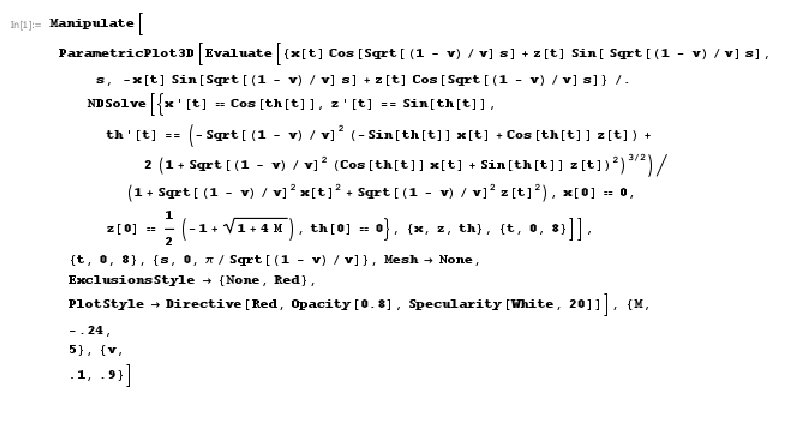
Let us start this section with some figures, most of them taken from animations created with Mathematica. The code that produced Figure 1.8 and the videos suggested in Figures 1.3, 1.6, 1.7, and 1.15 will be included at the end of the paper. The reason why this code works is developed throughout the paper.

In 1841 [2], Delaunay showed that if one roll a conic section on a line in a plane and then rotates about that line the trace of a focus, one obtains a cmc surface of revolution. When the conic is a parabola we obtaine a Catenoid, when the conic is an ellipse, the surface is embedded and it is called an undoloid and when the conic is a hyperbola the surface is not embedded and it is called a nodoid. The undoloids and nodoids are called Delaunay surfaces. Figure 1.1 illustrates the relation between the ellipse and the trace of its focus. Notice that only one focus is used to get the curve that needs to get rotated in order to generate an undoloid. Figure 1.2 illustrates the relation between the hyperbola and the trace of the foci. Notice that both foci are used to get the curve that needs to get rotated in order to generate a nodoid.

In 1970, Using the integrability of the Gauss Equation and Mainardi-Codazzi equation, Lawson showed that for any immersion $f_{0}:U\to{\bf R}^{3}$ with constant mean curvature $H$, defined in a simple connected surface $U$, there exists a $2\pi$-periodic 1-parametric family of immersions $\{f_{\theta}:U\to{\bf R}^{3}:\theta\in[0,2\pi]\}$ with constant mean curvature $H$ and with the same induced metric. The family $f_{\theta}$ is called the associated family to $f_{0}$.

In 1982 [1] Do Carmo and Dajczer studied surfaces with constant mean curvature that are invariant under the group $g_{t}:{\bf R}^{3}\to{\bf R}^{3}$ of rigid motions

They called these surfaces helicoidal with a pitch $h$. When $h=0$, the group $g_{t}$ becomes a group of rotations and the helicoidal surfaces become surfaces of revolution. Therefore, when $h=0$ the helicoidal surfaces are either cylinders, spheres or Delaunay surfaces. The main result in their paper established that every Helicoidal surface is associated with a Delaunay surface.

A Twizzler is an immersion of the form

with constant mean curvature. We will assume that the curve $(x(s),z(s))$ is parametrized by arc length and we will call it the profile curve of the Twizzler. Notice that Twizzlers correspond to those helicoidal surfaces with nonzero pitch.

In this paper we will give an interpretation of the profile curve of Twizzlers similar to the interpretation for the profile curves of the Delaunays. In order to do this, given a regular curve $\alpha$ in the plane, we define the TreadmillSled of $\alpha$ as the trace of the origin when this curve (and the plane that contains it) rolls on a treadmill located at the origin which is aligned along the $x$-axis. Notice that the origin, as a point in the plane that contains the curve $\alpha$, plays and important roll in this definition, for example, the TreadmillSled of a circle with center at the origin is just a point, while the TreadmillSled of a circle of radius $R$ whose center is at a distance $r$ of the origin, is a circle of radius $r$ with center $(0,R)$. Figure 1.3 shows the TreadmillSled of an ellipse with center at the origin. The black dot represents the center of the ellipse while the blue curve represents the trace of this center. As the next theorem shows, it turns out that for any curve $(x(s),z(s))$ parametrized by arc-length there is an easy expression for its TreadmillSled.

Notice that $(\xi_{1}(s),\xi_{2}(s))$ are the coordinates of the vector $(x(s),z(s))$ with respect to the orthonormal basis $\{(x^{\prime}(s),z^{\prime}(s)),(-z^{\prime}(s),x^{\prime}(s))\}$.

There is a relation between the profile curve of Delaunay surfaces and conics. For Twizzlers, there is a relation between their profile curves and the level sets of the function $h_{w}(x,y)=x^{2}+y^{2}+\frac{y}{\sqrt{1+w^{2}x^{2}}}$. It is not difficult to check that the range of the function $h_{w}$ is the interval $[-\frac{1}{4},\infty)$, that $h_{w}^{-1}(-\frac{1}{4})=\{(0,-\frac{1}{2})\}$ and that, every $M>-\frac{1}{4}$ is a regular value of $h_{w}$ and $h_{w}^{-1}(M)$ is a closed simple curve. We will refer to these level sets as heart-shaped curves. Figure 1.4 shows some of these level sets

The following Theorem establish the relation between the heart-shaped curves and the profile curve of the Twizzlers

The previous theorem is a consequence of the following proposition:

Figure 1.5 shows the profile curve of a Twizzler and the heart-shaped curve associated with it. Figure 1.6, is a picture showing how, for this Twizzler, the TreadmillSled of the profile curve is indeed negative the heart-shaped curve.

The following theorem gives us another application of the treadmillSled

Figure 1.17 shows how the TreadmillSled of the profile curve produces a vertical semi line.

If we exclude the cylinder and the value $M=-\frac{1}{4}$, Theorem 1.3 establishes a 1:1 correspondence between pairs $(M,w)$ with $M>-\frac{1}{4}$ and $w>0$ and Twizzlers with mean curvature 1. In order to deal with a bounded parameter, we will define $v=1/(1+w^{2})$, therefore, the parameter $v$ moves from $0$ to $1$ when $w$ moves from $\infty$ to $0$. Figure 1.7 shows pictures from an animation that produces a piece of the Twizzler associated with values of $M$ and $v$. We will refer to this Twizzler as $\mathfrak{T}(M,v)$ when the dependence of $M$ and $v$ is needed.

Explicit parametrizations for the heart-shaped curves make the understanding and drawing of Twizzlers easier. The following Lemma provides a possible parametrization for these heart-shaped curves.

We can define a fundamental piece of a profile curve as a connected piece of profile curve with the property that the TreadmillSled motion of this piece goes exactly once over the heart-shaped curve. It is not difficult to see that the whole profile curve is the union of fundamental pieces. Figure 1.8 shows the fundamental piece of the profile of a properly immersed Twizzler, along with the whole profile curve made up of four pieces in this case, and the graph of the Twizzler. For an undoloid we could define a fundamental piece as the trace of the focus of the ellipse when this ellipse rolls once. It is clear that the integers $\mathbb{Z}$ acts on the group of symmetries of the Delaunay surfaces in the form of translations. Theorem 1.8 shows that the group $\mathbb{Z}$ also acts on the set of isometries of Twizzlers.

In order to produced Figure 1.8, it was necessary to find a formula for the length of the fundamental piece of the profile curve. The following lemma provides such a formula.

The following theorem along with Theorem 1.12 and Theorem 1.13 give a precise picture of the Moduli space for the Twizzlers.

For a Twizzler that does not contain the axis of symmetry, the “properly immersed vs. dense” property established in the theorem above was proven by Hitt and Roussoss [4]. By numerically solving the equation $\int_{0}^{2\pi}\psi du=2\pi\,a/b$ in the previous theorem, we can graph profile curves of Twizzlers with any desire property. In Figures 1.9 we solve the numerical equation fixing $M=0$ and taking several integer values for $a$ and $b$. Since $M=0$, these profile curves represent twizzlers that contain the axis of symmetry. In Figure 1.10 we took several values for $M\neq 0$ and $a$ and $b$ integers to produce properly immersed twizzlers that do not contain the axis of symmetry. In Figure 1.11 we took $a$ and $b$ so that $a/b$ is not rational so that the twizzler is not properly immersed. In Figure 1.13 we took $a=5$, $b=4$ and 4 values of $M$ in order to produce properly immersed examples, we also show the points $(M,w)$ associated with these Twizzlers. Figure 1.12 shows the graph of the function $r_{1}(M)$ or $r_{2}(M)$ defined in Theorem 1.8.

By Dajczer and Do Carmo’s Theorem, we know that every Twizzler is isometric to a Delaunay surfaces, in order to decide which one, we will prove the following properties for Delaunay surfaces,

We have that the function $rs$ defines a bijection between the intervals $(-\frac{1}{4},0)$ to $(0,1)$ and also it defines a bijection between the intervals $(0,\infty)$ to $(0,1)$. On the other hand, each undoloid is isometric (associated with angle $\theta=\frac{\pi}{2}$) to a nodoid, see for example Appendix A in the paper [5] written by Kopouleas. As a consequence of Theorem 1.9 we have the following corollary:

As pointed out before, each nodoid is isometric to a undoloid, therefore we can replace the word Delaunay by either the word undoloid or nodoid in the Do Carmo-Dajczer theorem, that is, we can say that each Twizzler is isometric (or associated) to either a nodoid or an undoloid. Another family of surfaces that holds the same property is the set of Twizzlers that contains the axis of symmetry, that is, the set of Twizzlers corresponding to $M=0$ in the moduli space. We will call these surfaces special twizzlers and we will denote them by $\mathbb{S}\mathfrak{T}(v)$, that is, $\mathbb{S}\mathfrak{T}(v)=\mathfrak{T}(0,v)$.

The following Theorem gives us the quotient of the maximum value and the minimum value of the Gauss curvature for special Twizzlers.

Figure 1.15 shows two sets of isometric nodoid-undoloid-special Twizzler surfaces. We can generalize the theorem above as follows,

Since the curve $\alpha_{c}(M)=(M,\frac{\sqrt{1+4M}-1-2M+c(\sqrt{1+4M}+1+2M)}{\sqrt{1+4M}+1-2M+c(\sqrt{1+4M}-1+2M)})$ satisfies that $\alpha_{c}(-\frac{\sqrt{c}}{(1+\sqrt{c})^{2}})=(-\frac{\sqrt{c}}{(1+\sqrt{c})^{2}},0)$, $\alpha_{c}(0)=(0,c)$ and $\alpha_{c}(\frac{\sqrt{c}}{(1-\sqrt{c})^{2}})=(\frac{\sqrt{c}}{(1-\sqrt{c})^{2}},0)$  then, we have as a corollary of the previous two theorems and Remark 1.1 that

The continuity at the points of form $-\frac{1}{4}+\mathfrak{i}v$ follows from Theorem 1.8, because each Twizzler $\mathfrak{T}(M,v)$ is contained the region bounded by the two concentric cylinders of radii $r_{1}(M)=|\frac{\sqrt{1+4M}-1}{2}|$ and $r_{2}(M)=\frac{\sqrt{1+4M}+1}{2}$. Figure (1.17) shows the trace of the curve $\alpha_{u}$ for several values of $u$. As a consequence of the previous theorem we have that the family of associated surfaces $f_{\theta}$ for Twizzlers repeats every $\frac{\pi}{2}$. More precisely, it is $\pi$-periodic and it is 2:1 when defined in the interval $[0,\pi]$.

The author would like to express his gratitude to Professors Robert Kusner, Ivan Sterling, Bruce Solomon, Wayne Rossman, Martin Kilian and Ioannis Roussos for solving several of his doubts about Delaunays and Twizzlers and for providing him references.

In this section we will provide the proofs of the results established in the introduction. We will start with Theorem 1.2.

Proof Theorem 1.2: For every $s_{0}$ in the domain of the curve $\alpha$, we can find an isometry from ${\bf R}^{2}$ to ${\bf R}^{2}$ of the form $T{\bf x}=R(\gamma(s_{0})){\bf x}+c(s_{0})$ that rotates the curve $\alpha$ so that $\alpha(s_{0})$ moves to the origin and the vector $\alpha^{\prime}(s_{0})$ moves to the unit vector that points to the positive direction of the $x$ axis. Here

The angle $\gamma(s_{0})$ and the constant $c(s_{0})$ can be found by the solving the following equations (the solution of these equations is the key part of the proof of this theorem)

where $\beta(s)=R(\gamma(s_{0}))\alpha(s)+c(s_{0})$. If follows that the TreadmillSled of the curve $\alpha$ is the curve $c(s)$. A direct verification shows that

This completes the proof of the theorem.  

Proof of Proposition 1.4: Since the curve $(x(s),z(s))$ is parametrized by arc-length, we can consider a function $\theta(s)$ such that

Let us define the functions $\xi_{1}(s)$ and $\xi_{2}(s)$ as

A direct verification shows that

Moreover, it is not difficult to check that,

A direct verification shows that the first fundamental form of $\phi$ is given by

and therefore,

A Gauss map of the immersion $\phi$ is given by $\nu=\frac{1}{\sqrt{EG-F^{2}}}\,\phi_{s}\times\phi_{t}$. A direct verification shows that,

Again, a direct verification shows that the second fundamental form of $\phi$ is given by

Therefore, if we assume that the mean curvature $\frac{eG-2fF+gF}{2(EG-F^{2})}$ is 1 we obtain the following ODE

Using the expression above for $\theta^{\prime}$ in the equations $\xi_{1}^{\prime}=\theta^{\prime}\xi_{2}+1,\quad\xi_{2}^{\prime}=-\theta^{\prime}\xi_{1}$, we obtain that $\xi_{1}$ and $\xi_{2}$ satisfy the following ODE,

where,

A direct verification shows that if we define

then, $h_{w}$ is a first integral of the ODE for $\xi_{1}$ and $\xi_{2}$, i.e. for any solution $\xi_{1}(s)$ and $\xi_{2}(s)$ of this system, we have that

This completes the proof of the Proposition.  

Proof of Theorem 1.5: If we define the functions $\theta,\,\xi_{1}$ and $\xi_{2}$ as in the previous theorem, we have that the equation: Gauss curvature equal zero, that is, the equation $eg-f^{2}=0$ reduces to $\theta^{\prime}=-\frac{1}{\xi_{2}}$. Replacing this equation in the equations $\xi_{1}^{\prime}=\theta^{\prime}\xi_{2}+1,\quad\xi_{2}^{\prime}=-\theta^{\prime}\xi_{1}$, we obtain that $\xi_{1}$ and $\xi_{2}$ satisfy the following ODE,

It follows that $\xi_{1}(s)=\frac{a}{2}$ for some real number $a$. If $a=0$ then $\xi_{2}$ is also constant different from zero, and the surface $\phi$ is a cylinder. In the case that $a$ is not zero then $\xi_{2}=\pm\sqrt{as+b}$ and $\theta(s)=\mp\frac{2\sqrt{as+b}}{a}$. This completes the proof of the theorem.  

As mentioned before, Theorem 1.3 follows directly from Proposition 1.4. Lemma 1.6 is a direct computation.

Proof of Lemma 1.7 and Theorem 1.8: Let us start by pointing out that for any $M>-\frac{1}{4}$, the minimum and maximum distance from the origin to the set $h_{w}^{-1}(M)$ are $r_{1}(M)=|\frac{\sqrt{1+4M}-1}{2}|$ and $r_{2}(M)=\frac{\sqrt{1+4M}+1}{2}$ respectively. We can see this by using the method of Lagrange multipliers to find the maximum value and minimum value of the function $R(x_{1},x_{2})=x_{1}^{2}+x_{2}^{2}$ subject to the restriction $h_{w}=M$. We can prove that if $(x_{1},x_{2})$ is one of these critical points, then $x_{1}=0$ otherwise the equations

has not solution. Once we know that $x_{1}$ must be zero, we obtain from the equation $h_{w}=M$ that $x_{2}$ is either $-\frac{\sqrt{1+4M}+1}{2}$ or $\frac{\sqrt{1+4M}-1}{2}$. Let us continue with the rest of the proof. Let us assume that $(x(s),y(s))$ are such that the surface (1.1) has constant mean curvature 1. Since the curve $(\rho_{1},\rho_{2})$ defined in Lemma 1.6 is regular, we have that

is a periodic positive function. Likewise, since the functions $f_{1}(x_{1},x_{2})$ and $f_{2}(x_{1},x_{2})$ only vanish simultaneously at $(x_{1},x_{2})=(0,-\frac{1}{2})$, we get,

is a positive periodic function. Notice that $\xi_{1}(s)=0$ and $\xi_{2}(s)=-\frac{1}{2}$ is the only constant solution of the system (2.3). For any other solution, since $h_{w}$ is a first integral of the system, there exists $M>-\frac{1}{4}$ and a function $\sigma(s)$ such that

is a solution of the system (2.3). From the equations above we have

On the other hand we have that,

It follows that $\sigma$ is either strictly increasing or strictly decreasing, WLOG we can assume that $\sigma$ is strictly increasing. Therefore we get that,

If $\kappa(u)$ is the inverse of the function $\sigma(s)$, we have that

If we change from the variable $s$ to the variable $u$, that is, if we consider the functions,

It follows from Equation (2.6) and Equation (2.2), that

Since $\psi(u)$ is a periodic function with period $2\pi$, it follows by the existence and uniqueness theorem of ODEs that if $\tilde{\theta}(2\pi)=\theta_{0}$, then

Since $|(x(s),z(s))|=|(\xi_{1}(s),\xi_{2}(s))|$, we have that the piece of profile curve

References

- [1] Dajczer, M., Do Carmo, M. Helicoidal surfaces with constant mean curvature, Tohoku Math. Journal 34, (1982), 425-435.
- [2] Delaunay, C. Sur la surface de revolution dont la courbure mayenne est constante, J. Math. Pures Appl., Ser. 1 6, (1841), 309-320.
- [3] Lawson, B. Complete minimal surfaces in , Ann. Math. 92 (2), (1970) 335-374.
- [4] Hitt R., Roussos, I. Computer graphics of helicoidal surfaes with constant mean curvature, An. Acad. bras Ci., 63, (3), (1991), 211-228.
- [5] Kapouleas, N Constant mean curvature surfaces in Euclidean Three-Space, Annals of Math. (Ser 2) Vol 131 No 2, (1990), 239-330.
- [6] Konopelchenko, Taimanov Constant mean curvature surfaces via an integrable dynamical system, J. Phys. A: Math. Gen. 29, (1996), 1261-1265.