Quantum dot spin qubits in Silicon: Multivalley physics
Abstract
Research on Si quantum dot spin qubits is motivated by the long spin coherence times measured in Si, yet the orbital spectrum of Si dots is increased as a result of the valley degree of freedom. The valley degeneracy may be lifted by the interface potential, which gives rise to a valley-orbit coupling, but the latter depends on the detailed structure of the interface and is generally unknown a priori. These facts motivate us to provide an extensive study of spin qubits in Si double quantum dots, accounting fully for the valley degree of freedom and assuming no prior knowledge of the valley-orbit coupling. For single-spin qubits we analyze the spectrum of a multivalley double quantum dot, discuss the initialization of one qubit, identify the conditions for the lowest energy two-electron states to be a singlet and a triplet well separated from other states, and determine analytical expressions for the exchange splitting. For singlet-triplet qubits we analyze the single-dot spectrum and initialization process, the double-dot spectrum, singlet-triplet mixing in an inhomogeneous magnetic field and the peculiarities of spin blockade in multivalley qubits. We review briefly the hyperfine interaction in Si and discuss its role in spin blockade in natural Si, including intravalley and intervalley effects. We study the evolution of the double-dot spectrum as a function of magnetic field. We address briefly the situation in which the valley-orbit coupling is different in each dot due to interface roughness. We propose a new experiment for measuring the valley splitting in a single quantum dot. We discuss the possibility of devising other types of qubits in Si QDs, and the size of the intervaley coupling due to the Coulomb interaction.
I Introduction
A practical QC architecture requires scalability and long coherence times. Spin-based solid state quantum bits (qubits) are known to have long coherence times,[3, 1, 2] while also offering the promise of scalability, and are natural building blocks for quantum computation. The conventional criterion establishing an acceptable coherence time for fault-tolerant quantum computing is for it to allow operations. With the operation time set by the gating time ns the coherence time required is s.
Phosphorus donor nuclei in Silicon have been known since the 1950s to have some of the best spin coherence properties in solids,[3, 6, 5, 4] and were therefore proposed as viable candidates for qubits.[7] However, fabrication of ordered and gated donor arrays and coherent control over donor electrons has turned out to be extremely difficult (note nevertheless outstanding recent developments. [9, 8, 10])
Electron spin qubits in quantum dots (QDs), [11] particularly in GaAs, have been actively studied in the past decade, and coherence times in excess of s have been achieved.[12, 1, 2] Various schemes exist for implementing spin qubits in QDs. For the original single-spin qubits, one electron spin is initialized in each dot in a QD array,[11] with spin up and down representing the two states of a qubit. One-qubit rotations are accomplished using magnetic resonance techniques and two-qubit rotations by means of a pulsed exchange interaction. One can also use selected two-spin states to encode a logical qubit: in singlet-triplet qubits it is the singlet and unpolarized triplet states that are used for encoding. Here exchange coupling gives the splitting of the two-spin states making up the qubit.[14, 1, 13] One-qubit rotations are currently carried out using an inhomogeneous magnetic field across the two dots and pulsed exchange splitting. Two-qubit operations use the different dipole moments of the singlet and triplet states. [13] Larger encoding schemes such as using three-spin states have also been proposed,[15] aiming at an all-electrically-controlled architecture.
Recent years have seen significant experimental progress involving single-spin properties such as coherent control, coherence, and measurement.[16, 17, 18, 19, 4, 20, 21, 2, 22, 23] In GaAs double quantum dots (DQDs) spin blockade [16] and charge sensors (quantum point contacts and radio-frequency quantum point contacts)[24] enable observation of single/two-spin dynamics.[1, 19, 2, 25, 4] Spin coherence in GaAs QDs is mostly limited by hyperfine interaction with the nuclear spins,[26, 27, 28, 29, 30, 31, 32, 33, 34] though proposals exist for manipulating nuclear spin states to extend electron spin coherence times,[35, 36, 37, 38] and recent experiments[12, 1] have shown that dynamical decoupling schemes [29, 39, 40, 41, 42, 34] could help unwind the nuclear spin dynamics. Progress has also been made on controlling spins in GaAs QDs by optical means, such as the preservation of spin coherence,[43] control of the nuclear spin polarization, [44, 45, 46] and ultrafast spin rotations.[47] Yet experiment is far from achieving reliable control over the nuclear field in GaAs.
Silicon has outstanding spin coherence properties [3] due to small spin-orbit coupling,[48] small hyperfine interaction with nuclear spins[49] (which can be reduced by isotopic purification [50]) and absence of piezoelectric coupling.[51] The spin coherence time (after Hahn spin echo) for donor electron spins in bulk Si:P has been reported to range from 60 ms [5] to 300 ms. 11 1 S. Lyon, private communication This is the longest coherence time measured in electron spin qubits, and greatly exceeds the values reported in GaAs QDs, which, after Hahn echo, range from s [1, 2] to s.[12] Isotopic purification of Si, where 29Si nuclei are preferentially removed in favor of 28Si and 30Si nuclei from natural Si, allows enhancement of Si electron spin coherence times.[52, 5] The maturity and continuous innovation in Si microfabrication could be of great help in scaling up a Si-based QC architecture. Work is under way on Si QC architectures based on donor electron or nuclear spins in a Si:P system,[7, 53] single electron spins in gate-defined quantum dots in Si/SiGe[54, 55] or Si/SiO2,[56, 57, 58] and holes in SiGe nanowires.[20] Experimental progress has been made in both donor-based devices[59, 60, 61, 62, 63, 64, 65, 9, 8, 10], and gate-defined QDs. [66, 67, 21, 56, 57, 8, 10, 68]
The valley degree of freedom presents a potential obstacle to spin QC in Si. In bulk Si there are six degenerate conduction band minima near the X points in the first Brillouin zone. Impurity scattering breaks the symmetry of the lattice and allows coupling between the valleys, and in samples in which two or more donor centers are present interference becomes possible and is sensitively dependent on the exact atomic locations of the two donors. [69, 70, 71] Confinement in the -direction and/or uniaxial tensile strain at the interface cause the valleys perpendicular to the interface to have a smaller energy by several tens of meV than the valleys in the plane of the interface. A sharp interface further couples the two -valleys by producing a valley-orbit coupling (a complex number). [72] is generally not known a priori, is sample-dependent, [73] and is different for different interfaces, such as Si/SiGe and Si/SiO2. Various measurements of have been reported, [76, 74, 75, 67] and efforts have been devoted to calculating . [77, 81, 73, 78, 54, 79, 80] Yet the fact that is not known and no standard experiment exists to measure it in a QD at low field is a strong motivating factor for our work.
| (a) |
 |
| (b) |
 |
In a recent article [82] we discussed singlet-triplet qubits in Si QDs, emphasizing the role of the valley degree of freedom. The focus of Ref. 82 was on determining the feasibility of an experiment analogous to Ref. 1 in a Si/SiO2 (or Si/SiGe [21]) DQD. It was found that the valley degree of freedom affects qubit initialization, operation and spin blockade. For a singlet-triplet qubit can be implemented in the same way as in GaAs. For initialization will be problematic, since, unlike in GaAs, the energy scale is no longer set by the confinement energy but by the valley splitting (we note a similar discussion of spin blockade in carbon nanotube quantum dots.[83, 84])
In this work we present a detailed analysis of both single-spin and singlet-triplet qubits in multivalley Si QDs within the effective mass approximation. The discussion of valley physics is general and applies to all types of Si QDs, yet when concrete figures are needed we focus on Si/SiO2. Many aspects of the following considerations apply also to carbon-based QDs, where the valley degree of freedom is present as well. [85, 83, 84] We consider first single-spin qubits, i.e. the Loss-DiVincenzo (LDV) architecture.[11] We determine the spectrum and the conditions required for implementing single-spin qubits and coupling adjacent qubits by means of the exchange interaction. We subsequently study singlet-triplet qubits.[1, 13, 82] Part of the discussion is intended as a follow up to Ref. 82, providing further theoretical details of singlet-triplet qubits including all the relevant analytical formulas and matrix elements. The remainder contains an extensive discussion of the role of the hyperfine interaction in spin qubits in natural Si, including intervalley effects, an exhaustive discussion of single-qubit gates and scalability, as well as new experimental initiatives. We conclude that in both schemes, for any , single-qubit operations are feasible. If in single-spin qubits exchange-based entanglement will not work since exchange between pairs of states with different valley composition is vastly different. For this reason, the proposed Coulomb interaction-based two-qubit operations in the singlet-triplet scheme will not work either.
The outline of this article is as follows. In Sec. II we introduce the DQD Hamiltonian. In Sec. III we study the effect of the valley degree of freedom on single-spin qubits and in Sec. IV we investigate singlet-triplet qubits and the role of the valley degree of freedom in initialization, coherent manipulations, and readout. We give a brief review of hyperfine interactions in Si, then discuss intravalley and intervalley effects relevant to singlet-triplet qubits. Interface roughness is discussed in Sec. V, other types of qubits in Sec. VI, and in Sec. VII an experiment is discussed that can estimate the valley splitting. We also discuss briefly the effect on spin qubits of interface roughness, which may lead to a different valley-orbit coupling in the two dots. We end with a summary and conclusions.
II Model of a double quantum dot
We focus on a DQD in a two-dimensional electron gas (2DEG) in the inversion layer of a MOSFET grown along the -direction (which is also the crystalline (001) direction). The dots are located at , where , and while (since the and valleys are isotropic in the plane, we can choose the and axes by convenience). We do not consider spin-orbit interactions. The DQD Hamiltonian , where represents the valley-orbit coupling discussed below and , where is the kinetic energy operator and the confinement potential
| (1) |
with and the Fock-Darwin radii for in- and out-of-plane confinement respectively. The external electric field is used to bias the DQD and is a crucial tuning knob for singlet-triplet qubits. The Coulomb potential between electrons at and is , where the effective dielectric constant accounts for the extra screening due to the image charge in SiO2 (for Si/SiGe such averaging is not needed). We use a quadratic potential to model the growth-direction confinement, which is generally triangular. The in-plane confinement potential for each dot is harmonic near the center, , with Gaussian ground states.
The confinement along the growth direction splits the six-fold degenerate Si conduction band into a doubly-degenerate branch of lower energy and a fourfold-degenerate branch of higher energy. The two lower energy valleys are along the direction perpendicular to the interface at , where , and the lattice constant . The ground-state wave functions satisfy , with
| (2) |
where or . The envelope functions are
| (3) |
where is the in-plane Fock-Darwin radius, , the growth-direction confinement length, is the in-plane (transverse) Si effective mass, and the bare electron mass. The lattice-periodic function , with the reciprocal lattice vectors.
Overlaps of the form are given by , where . Overlaps of the form are suppressed by an exponential of the form , where ( is an integer). With nm typically,[76] when and when . Matrix elements of potentials smooth in space and interactions between states from different valleys are suppressed by such prefactors: matrix elements of the form and . The one exception is the valley-exchange Coulomb integral below. Two-particle matrix elements in which each electron belongs to a different valley, for example , are of the same order of magnitude as those in which all functions belong to the same valley, such as . Matrix elements of interactions on the atomic length scale are not exponentially suppressed. One prominent example is the hyperfine (hf) interaction between a conduction electron and a 29Si nuclear spin (in a natural Silicon substrate about 4.7% of the nuclei are 29Si).
Based on multiple experiments conducted over the past 50 years and on the recent calculations (see Sec. IV.2.4 for details), it is assumed that the hf interaction in Si is dominantly of the contact character, i.e. the Hamiltonian is given by
| (4) |
where the sum runs over the positions of the 29Si nuclei, (with and being the electron and nuclear gyromagnetic factor, respectively), is the unit cell volume and are the nuclear spins. The valley-diagonal matrix element is
| (5) |
where the hf interaction energy is with , see Ref. 49 and references therein ( eV in Si). This Hamiltonian provides a valley-orbit coupling mechanism, i.e. we have . The consequences of this coupling are explored below.
The interface potential couples the and valleys if it is sufficiently sharp on the atomic scale. This is contained in , which represents the valley-orbit coupling studied in detail recently.[77, 73] The magnitude and phase of are of great interest in Si research. It has been shown that can range from zero to 0.25 meV (maybe even larger),[77, 81] and both its magnitude and phase can be controlled by an electric field. In the present work is a single-particle phenomenological coupling between the valleys , with . Throughout this work .
We diagonalize the single-particle Hamiltonians including and obtain the valley eigenstates with eigenvalues in each of the quantum dots. We construct orthogonal (Wannier) single-dot wave-functions [86] and , where , so that . We define
| (6) |
Orthogonalizing and we obtain and . These are the single-electron states we will use henceforth (e.g. to construct two-electron states.) The orbital excitation energy is assumed large ( 1meV, or .)
III Single-spin qubits
For single-spin qubits we first consider initialization. In single-valley systems the lowest energy level in zero magnetic field is spin-degenerate but orbital-non-degenerate. Initialization of a definite single-spin state requires a magnetic field to split the spin degeneracy via the Zeeman interaction, so that selective tunnelling from a reservoir can have high fidelity.[17] Experimentally in GaAs this process requires magnetic fields of several Tesla due to the inherent smallness of the Bohr magneton, the small -factor in GaAs (), and the constraint of 100 mK electron temperature in the reservoir. In Si , so that at dilution refrigerator temperatures much smaller magnetic fields will be required than in GaAs, rendering spin initialization a relatively simple task.
In Si however there are two possibly closely-spaced one-electron levels and , separated by . Initializing into a definite orbital state is dependent on the size of . Since the interaction of spins in states and with a magnetic field is described by identical Zeeman Hamiltonians, single-qubit rotations can be performed no matter which state is initialized.
III.1 Two-qubit gates
In the LDV architecture two-qubit gates are implemented using the exchange interaction between neighboring dots. Two-electron wave functions are superpositions of spin singlet and triplet states. Singlet wave function , where is a two-particle spatially symmetric function and is the two-spin singlet state given by . The superscript here denotes the -th electron. Triplet wave functions , where is a two-particle spatially antisymmetric function, and represents the spin-triplet states, and is an abbreviation for , , and . The wave functions represent the polarized spin triplets and are given by and respectively, while represents the unpolarized spin triplet and has the form . We will frequently refer to just and as the singlet and triplet states respectively, because the orbital part is where valleys play an important role.
Translating the LDV architecture to multi-valley systems requires taking into account the valley degree of freedom in the construction of many-particle wave functions. In general, for a given number of orbital states one can form singlet and triplet two-electron states. In a single-valley system the number of orbital states is , resulting in the trivial case of one singlet. In a single Si QD we have . For two electrons we have 2(2+1)/2 = 3 singlet states and 3[2(2-1)]/2] = 3 triplet states. In a Si double dot, when considering the lowest orbital state in each valley, , so that there are 4(4+1)/2 = 10 singlet states and 3[4(4-1)]/2 = 18 triplet states. Therefore there are altogether 28 states for the double dot, of which 10 are spatially symmetric (spin singlets) and 18 are spatially antisymmetric (spin triplets). The total number of 28 states corresponds to the combination , where arises as the product of a factor of 2 for the spin degree of freedom, a factor of 2 for the valley degree of freedom and a factor of 2 for the two dots. The combination is thus the number of combinations to construct a two-electron wave function out of 8 possible states, and represents the dimensionality of the representation of the permutation group on the combined two-dot two-spin two-valley SU(2)SU(2)SU(2) Hilbert space.
The singlet and triplet states in a Si DQD can be divided into three branches: states with the same valley composition, comprising wave functions of the form () and (), and states with mixed valley composition, comprising wave functions of the form (). There are thus in total six uncoupled branches, which can be labeled , , and , , (see Table 1.) The spatial parts of the singlet and triplet states are
| (7) |
For the states, the spatial parts of the singlets are
| (8) |
while the spatial parts of the triplet states are
| (9) |
Because we are using the Wannier states , there are no overlaps such as . The spatially symmetric functions split into three single-valley states from the lower-energy branch, three single-valley states from the higher-energy branch, and four states from the branch. The spatially antisymmetric functions split into one single-valley state from the lower-energy branch, another single-valley state from the higher-energy branch and four states from the branch.
As we discussed before, the smooth quantum dot confinement potential and the electron-electron Coulomb interaction do not introduce further transitions between valleys (the matrix elements are mostly exponentially suppressed, and the only Coulomb matrix element that is not exponentially suppressed is nonetheless very small, as we show in the Appendix). Thus the , and branches do not mix, allowing us to analyze them separately.
The two-electron Hamiltonians in the branches, in the bases , have the form
| (10) |
All terms are given in the Appendix. In the branch,
| (11) |
where applies to and to , and is in the basis while for replace . Since the overlap between states from different valleys is negligible, matrix elements of the form and are equal up to a sign (we will discuss below the case when this condition is not satisfied.) The eigenvalues of and are exactly the same. In other words, there is no exchange splitting between the singlet and triplet states if the two electrons are in different valley eigenstates.
III.2 Scalability
The structure of the two-electron Hamiltonian has important consequences for the operation of spin qubits in silicon. The and branches have the same structure as the single-valley Hamiltonian except they are shifted up and down by respectively. These branches can be regarded as replicas of the usual single-valley Hund-Mulliken Hamiltonian.[87, 86] The singlet and triplet states have the same form as in the single-valley case. The principal difference from the one-valley situation emerges when we consider the branches, where we have four sets of degenerate singlet and triplet states. This degeneracy is the direct manifestation of the fact that exchange integrals for electrons from different valleys vanish (either exponentially small or very small due to Bloch function symmetry, see Appendix).
The essence of exchange gates in the Loss-DiVincenzo architecture is the control of the phase difference (introduced by a finite exchange splitting) between singlet and triplet states. In the or branches the two electrons are in the same valley eigenstate, so that we exactly recover the single-valley physics of GaAs, and exchange gates can be implemented. However, in the and branches singlet and triplet states are degenerate, rendering exchange gates impossible. Now assume that the two electrons were initialized into two initially independent quantum dots with an arbitrary combination of valley eigenstates. When the inter-dot barrier is lowered, if is sufficiently small, the two-electron states would generally populate all four branches (, , , and ). Since exchange gates cannot be implemented in the and branches, they cannot be implemented for these two electrons in general. The only way to perform exchange gates is to have the two-electron states populating only the and branches. With the electrons in a reservoir in a structure-less Fermi distribution, the only single-electron state that can be loaded exclusively is the valley eigenstate (if ), so that when inter-dot tunnelling is turned on, the two electrons are in the branch. This is the only viable option where exchange gates can still be performed. The exchange splitting between the lowest-lying singlet and triplet states in the branch is given by the Hund-Mulliken expression,[86, 88] which can be obtained by straightforward diagonalization of Eq. (10),
| (12) |
In the and branches there are four energy levels: a singlet, a triplet which is higher by , and two singlets which are much higher in energy due to the on-site Coulomb interaction. In the branch one has the same four levels (bar the valley splitting), except that for each energy there is a singlet and a triplet. In this branch exchange is zero, and the next highest state is separated by . Therefore exchange in the three branches is either or zero. This fact becomes important when . Firstly, for , the lowest state is a (sixfold) degenerate singlet/triplet. For nonzero but , one may in general initialize a superposition of states and exchange is not well defined. Consider two qubits and . If the states are and , and the exchange coupling between them is zero. For arbitrary , exchange depends on the specific values of and and cannot be controlled, precluding QC operations.
Our analysis shows that in the LDV architecture for multivalley systems single-qubit operations are straightforward, while exchange-based two-qubit operations are not feasible unless . The optimal strategy is to strive to obtain a large valley splitting and work towards replicating the single-valley situation.
IV Singlet-triplet qubits
We have studied the implications of multiple valleys on the implementation of singlet-triplet qubits in Ref. 82. In this Section, aside from reviewing initialization (Sec. IV.1), we provide the important technical details and explore new features such as the evolution of the spectrum as a function of magnetic field, intravalley and intervalley effects due to the hyperfine interaction, the role of these terms in the dynamics of singlet-triplet qubits, the difference between applied and hyperfine magnetic fields, spin blockade and two-qubit operations.
We use the notation (,) to indicate the occupancy of the left and right dots respectively. The single-particle energies on the left and right dots are different, and . The dimensionless detuning is defined as , and the dimensionless critical detuning .
 |
IV.1 Initialization
Our study of the singlet-triplet qubit follows the successful experimental implementation in GaAs DQDs, which has 4 basic ingredients: initialization in a single dot in the (0,2) regime, single-qubit manipulation in the (1,1) regime, two-qubit manipulation via electrostatic interaction, and spin measurement via spin blockade. [1, 25]
First a (0,2) state is initialized (.) Using the notation of Sec. III, the four lowest-energy two-particle spatial wave functions are,
| (13) |
In the basis the Hamiltonian is
| (14) |
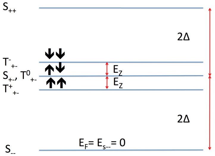
For and no external magnetic field , all six lowest-energy levels are degenerate and it is not possible to load any particular two-electron state. An external magnetic field splits the triplet energy levels by the Zeeman energy (Fig. 2.) Initialization of a (0,2) state requires an outside reservoir with a Fermi energy (thermally broadened by ) tuned to be on resonance with . If (at T=100mK we require 0.1meV) then can be loaded exclusively.
The qubit of Refs. 1, 4 is in a single-valley system, so . Only a singlet can be made out of the lowest lying wave function. The triplet involves higher orbitals and is separated by , minus a small exchange term. In GaAs this energy scale is 1 meV, which is much greater than the experimental thermal energy of 0.01 meV (100mK). In Si the energy scale is set by . If is sufficiently large the physics is that of a single-valley problem.
IV.2 One-qubit manipulation
Single-qubit operations on the singlet-triplet qubit are performed in the (1,1) regime.[1] The two-particle states are the same as those enumerated in the case of single-spin qubits, except here we do not include the high-energy (2,0) states of the form (see Table 1.) In the bases the matrix elements of the Hamiltonian in the branches are given by
| (16) |
The matrix elements in the branch, in the bases and , are
| (17) |
where the signs apply to the singlet/triplet Hamiltonians respectively.
The singlet and triplet branches always yield the same energies. Moreover, for the lowest energy state is sixfold degenerate: the lowest energy , and singlets, plus the lowest energy triplet. When the two electrons are in the same valley, the singlet and triplet energies differ by .
For clarity we focus on a concrete example, taking a Si DQD with a=8.2nm, b=3nm, d=2.45 and =0.1meV. The energy levels of the system with these parameters are plotted in Fig. 3 (analogous to Ref. 82) as a function of the dimensionless detuning . At low detuning there are four (0,2) high-energy levels, indicated by the two solid lines (representing singlets of the form , ) and one dashed line (representing two degenerate singlet and triplet of the form ). The separation of these levels is 2. The lower-energy (1,1) levels are a degenerate singlet/triplet of the form (top solid line), a degenerate singlet/triplet of the form (bottom solid line), and two degenerate valley mixing singlets and triplets of the form and . For the parameters considered in this example 0.02meV, giving a splitting at the avoided crossing of 0.06meV.
IV.2.1 Double dot spectra in different parameter regimes
Up to now we have considered the simplest form of the two-dot spectrum, which occurs in the case when is the largest energy scale, exceeding the tunnel coupling and the Zeeman splitting due to the uniform magnetic field by a noticeable amount. Yet it is evident that the qualitative features of the spectrum are sensitively dependent on the relative size of , , and . As these parameters vary with respect to one another, the relative position of most energy levels can differ greatly. As a result, there can be substantial variation in the loading and mixing dynamics of the two-electron states (Figs. 3–7.)
In Fig. 3 we plot the two-electron spectrum of a Si DQD when including all the Zeeman-split levels. It is interesting to follow the evolution of the two-dot two-electron spectrum as the ratio of the magnetic field to the valley splitting goes from small to large. This can be done by observing the way the spectrum changes from Figs. 3 through 6. These figures taken together illustrate the fact that, as the magnetic field increases with respect to the valley coupling there is a transition between the valley physics (which is in effect a pseudospin) and the Zeeman physics (which is due to the real spin). For large valley/Zeeman splitting the spectrum looks effectively the same, except in one extreme case the splitting between the three sets of levels is determined by whereas in the other extreme case it is determined by .
On the other hand Fig. 7 contains the two-dot spectrum for the opposite case when . In Figs. 3 and 7 we have assumed the same value of the Zeeman splitting. Finally, in general case one should be prepared for an intermediate scenario as in Fig. 5 in which the sets of levels are not clearly separated and may cross. In such a situation distinguishing the energy levels experimentally may prove challenging.


IV.2.2 Inhomogeneous magnetic fields in Si
Quantum coherent single-qubit experiments on singlet-triplet qubits make use of an inhomogeneous magnetic field. As shown in Ref. 1, an experiment on the singlet-triplet qubit often requires two magnetic fields: a uniform one to separate out the polarized triplet states, and an inhomogeneous one to mix the singlet and the unpolarized triplet states. In the existing experiments on GaAs[1] the latter is provided by the lattice nuclear spins.[89] In Si, hyperfine interaction is much weaker, and number of lattice nuclear spins much smaller.[49] Natural Si has only of the 29Si isotope having nonzero nuclear spin (28Si has no nuclear spin) and it can be further isotopically purified to nearly completely eliminate the nuclear spins. For the case when the inhomogeneous effective field arises from hyperfine interaction with the nuclei in the dots, the magnetic fields on the left and right dots ( and below) differ by a small amount of the order of where is the hyperfine constant of the material and is the number of nuclei interacting appreciably with the electrons. In gated GaAs QDs this amount is on the order of mT. In a natural Si QD it has been estimated to be in the range 0.06-6 neV, corresponding to a time scale of 0.1-10s and magnetic fields of 0.5-50 T, depending on the percentage of 29Si in the material, from 0.01 to 100.[49] In systems based on purified Si, an external inhomogeneous magnetic field must be generated, such as by a nanomagnet,[90] allowing better control. For example, one can tailor the inhomogeneous field to have only a -component with a gradient along the -direction.
Each initialized (0,2) state has a probability of return to the original state after staying for a certain time in the (1,1) regime. In a random hyperfine field this probability of return is determined by the nuclear spin polarization difference between the two dots. Since the experiment is repeated many times in the time domain, the observed results involve averages over the inhomogeneous nuclear field. On the other hand, in an applied inhomogeneous magnetic field, the field is the same during each experimental run. Therefore, by controlling the magnitude and orientation of the applied inhomogeneous field one can control the composition of the (1,1) state after mixing, and therefore the return probability. In this case, if the initial state is known, we have a controlled return probability. The key fact is that, in the far-detuned (1,1) regime where , each unpolarized state (singlet or triplet) mixes with one other unpolarized state, while polarized triplets do not mix with any other state (see Sec. IV.2.3). Knowledge of the controlled return probability requires exact knowledge and control of the applied inhomogeneous magnetic field inside each dot.
IV.2.3 Singlet-triplet mixing in an applied inhomogeneous magnetic field
The inhomogeneous magnetic field is the sum of nuclear and applied fields, . Experimentally one cannot generate an applied field with a profile sufficiently sharp in the -direction to mix states from different valleys, so for the Zeeman Hamiltonian does not mix and states. In the case of the nuclear field, the contact hyperfine interaction is a sum of -functions, and can mix states from different valleys. Here we consider . Considerations specific to are discussed in the following section.
The Zeeman Hamiltonian in Si, where approximately, for two electrons in a DQD is
| (18) |
where the spin operators act on the spin of particle 1 and 2 respectively. We study the Zeeman Hamiltonian in the subspace of two-electron (1,1) states formed out of the wave functions , which is relevant to operations on singlet triplet qubits. Its expectation values contain expressions of the form (assuming weak tunnel coupling)
| (19) |
We write these (real or effective) magnetic fields in the form , where the total magnetic field is and the field difference is . Here, since , the magnetic field is smooth in space and has no matrix elements between states and . In this case, since , the matrix elements of the Hamiltonian between the states are easy to find using Eq. (19)
| (20) |
Within the mixed-valley branch, neither an applied field nor the nuclear field can mix states with states in the mean field regime. We only consider the matrix elements of the Zeeman Hamiltonian within each branch of the two-dot spectrum, i.e. , and .
Singlet-triplet mixing occurs in the (1,1) configuration, when .[25, 1] Without putting in valley eigenstate indices, we are interested in the effect of the Zeeman term in the space of states spanned by a (1,1) singlet and a (1,1) triplet . An applied uniform magnetic field separates the polarized triplet states energetically, so that the two-electron system remains in the branch spanned only by and , where
| (21) |
We note that
| (22) |
and the off-diagonal matrix element is
| (23) |
The - and -components of mix the singlet with the polarized triplets
| (24) |
The polarized triplets are split off by the uniform Zeeman field and transitions to them are suppressed. The triplets are mixed among themselves by the total magnetic field
| (25) |
The uniform Zeeman field also suppresses this mixing. In an applied uniform magnetic field mix only with , and mix only with . Each unpolarized (1,1) state only mixes with one other unpolarized (1,1) state, which is important in spin blockade.
IV.2.4 The hyperfine interaction in Si
The hyperfine interaction between electron and nuclear spins in Si is relatively well known. For donor-bound electrons, the full hyperfine matrix, including both the contact and anisotropic hyperfine couplings to the donor nuclei and the 29Si nuclear spins in the environment, has been carefully measured and calculated.[3, 91, 92, 93] The thorough understanding of that problem allows quite precise knowledge of the coupled electron-nuclear-spin dynamics in Si:P, as represented by the impressive agreement between theory and experiment in ESR experiments on Si:P.[50] The hyperfine interaction with conduction electrons in Si is generally known to be weak relative to confined donor electrons. The earliest experimental measurement of hyperfine coupling strength for conduction electrons in Si dated back to the 1950s and 60s. [94, 95, 96] The contact hyperfine interaction, measured by average electron probability at nuclear sites, ranges from 178,[95] to 300[96], as compared with for GaAs.[97]
The study of hyperfine interaction in Si is currently drawing renewed interest because of the possibility of realizing spin qubits in Si. For example, in Ref.49, an all-electron calculation was performed to obtain the complete hyperfine coupling matrix (both contact and anisotropic parts). We note that the pseudopotential method is not appropriate for calculating contact hyperfine interaction because it fails at the nuclear sites, making the use of an all-electron calculation necessary. The calculated is about 160, consistent with experimental observations. Furthermore, the calculated anisotropic hyperfine coupling strength is about 3% of the contact part. The finite contact hyperfine coupling strength is a reflection that there is a finite component of atomic S-orbitals in the Bloch function at the bottoms of the Si conduction band, even though the Bloch functions are predominantly P-like. The small calculated anisotropic hyperfine coupling strength is a reflection of the highly symmetric nature of the Si lattice, in contrast with one-dimensional and two-dimensional structures such as carbon nanotubes and graphene sheets. In short, hyperfine interaction in Si is an extensively studied subject, with its magnitudes in various situations already measured and calculated.
An interesting contrast can be made between the hyperfine interactions in silicon and low-dimensional carbon structures, such as graphene. We recall that the conduction band minima in Si are located at along the (100), (010), and (001) axes. The six valleys are in the vicinity of the X points, which are high-symmetry points, but not at the X points themselves. Group theory tells us that the Bloch functions near the X points are P-like. Similarly, the Bloch functions near the conduction band minima are predominantly P-like, but with S-like and D-like admixtures.[98] Nevertheless, group theory itself does not yield the weight of these admixtures, and numerical calculations are required.
In contrast, the valleys in graphene are located at the high symmetry points and in reciprocal space, where group theory tells us the Bloch function are P-like.[99] When this is the case the contact hyperfine interaction vanishes. The dominant hyperfine contribution arises from the anisotropic part of the interaction. This fact has interesting consequences for spin blockade, which were explored in Refs. 83, 84. Despite the many similarities between Si and C, since the valleys in Si are not located at high-symmetry points, symmetry places no additional constraints on the form of the wave functions. In short, unlike in graphene, the contact hyperfine interaction in Si is finite,[49] and it actually dominates over the anisotropic interaction.
For the present purpose, namely understanding the effect of the hyperfine interaction on spin and valley dynamics of singlet-triplet qubits in Si quantum dots, it is sufficient to think of the hyperfine coupling as the interaction between an electron spin and an inhomogeneous Zeeman field. Both the contact and the anisotropic terms can be cast in this form. This field will in general differ between adjacent quantum dots, giving rise to singlet-triplet mixing when two states are close together in energy. The hyperfine interaction can in principle mix singlets and triplets with the same valley composition as well as singlets and triplets with different valley composition. These cases will be examined in what follows. We reiterate that any unwanted mixing present in natural Si can be eliminated by isotopic purification.
IV.2.5 Hyperfine-induced valley mixing
We write the contact hyperfine Hamiltonian in Si as
| (26) |
where the hyperfine magnetic field can be written as
| (27) |
The contact interaction can mix states of different valley compositions. The dipolar hyperfine (anisotropic) interaction for conduction electrons in Si is two orders of magnitude smaller,[49] so we neglect it for the following discussion. We again assume that a homogeneous magnetic field that is much larger than the nuclear field is applied so that we can neglect mixing with polarized triplet states. In other words, we only consider mixing of and here.
The intravalley matrix elements of the hyperfine interaction have the same form as those given above for the applied field. We also have the intervalley term
| (28) |
Since we are neglecting terms of the form and terms of linear and higher order in and , and we will write e.g. :
| (29) |
In this work we take and as given. These quantities can be determined by explicit evaluation of the matrix elements of as given in Eq. (27) using the wave functions introduced in Sec. II, yielding
| (30) |
Beyond this level the coefficients in the expansions of the Bloch functions need to be determined. Very recently has been worked out in Ref. 49, which demonstrated that the contact hyperfine interaction is finite in a Si QD. [49]. Explicit evaluation of requires more work. However, inspecting Eq. (30) we expect most of the contribution to to come from the term with . On the other hand in the term will be much smaller, due to the modulation introduced by the fast oscillating factor . The sum over will bring this term very close to zero, so that we expect . We stress that, since we take these quantities as given (as indeed we do with ) we make no assumptions about the form of the Bloch functions in Si appearing in these matrix elements (except for the assumption that the contact hf interaction is the dominant one).
We have the following interbranch matrix elements
| (31) |
In the matrix elements above the singlet and triplet labels could be reversed and the value will remain the same. Doing this for the first matrix element we obtain , and likewise for the subsequent ones. The hyperfine interaction does not mix the and branches directly. Within the branch we have the intervalley matrix elements
| (32) |
The states and are defined in the following Section. Unless specified otherwise, all remaining matrix elements are zero.
IV.3 Spin and valley blockade in multi-valley Si QDs
Spin blockade allows charge sensors (quantum point contact or single-electron transistor) to differentiate the two-electron singlet and triplet states.[16, 4, 1] In this subsection we explain the details of state mixing in the branches, and the reason an inhomogeneous magnetic field leads to spin blockade of only certain states. We also consider spin blockade in a hyperfine field, which has matrix elements between different valleys, and study their effect on singlet-triplet qubit operation.
Spin blockade occurs when the electrons occupy the (1,1) state with spin/valley structure incompatible with the structure of available (0,2) states. In such a case upon changing the detuning from the (1,1) regime to the nominally (0,2) regime tunneling of electrons into the right dot is suppressed, and the charge state of the DQD remains as (1,1). In the single-valley case this happens when we have a (1,1) triplet, which is lower in energy compared to the (0,2) triplet state after changing the interdot detuning to the detection regime, where the (0,2) singlet is the ground state. Therefore an initial (1,1) singlet state evolves to (0,2), while the (1,1) triplet state stays in the (1,1) configuration. This difference in the charge distribution can be detected by a charge sensor. In the multi-valley case the situation is more complicated.
We first consider an applied inhomogeneous magnetic field, and study the branches, which is described by the Hamiltonian . For the eigenstates are , and . As the detuning is swept adiabatically from to , the singlets evolve into , while the triplets remain unchanged: the (1,1) singlet evolves into the (0,2) singlet, while the (1,1) triplet remains in the (1,1) configuration, as in GaAs.
In the branch, spin blockade is rather subtle and interesting. Consider the singlet branch [ of Eq. (17).] The eigenstates in the (0,2) and the far-detuned (1,1) regimes are respectively and
| (33) |
In the regime of , only and are tunnel-coupled. Therefore, as the detuning is swept from to , the ground state evolves from into , while remains unchanged. For the triplet branch [ of Eq. (17)], the eigenstates in the far-detuned regimes of and are and
| (34) |
As the detuning is swept from to , the anti-symmetric state evolves into while remains unchanged. This is the opposite of what happens in the singlet branch.
Operation of the singlet-triplet qubit entails initialization of a unique (0, 2) state. When is initialized and the detuning is swept from to , this state evolves into . Under the action of an applied inhomogeneous magnetic field this state can only mix with the triplet . On the other hand, when is initialized and the detuning is swept from to , this state evolves into , which, in an inhomogeneous magnetic field, can only mix with the triplet . It is the same component of the inhomogeneous magnetic field that mixes with and with . We may refer to this process as valley blockade, similar to that seen in carbon nanotube QDs.[83, 84] As we sweep the detuning and allow states to mix, the destination (1,1) states ( and ) do not tunnel couple back to the (0,2) configuration, so that they are blocked. This should then allow a charge sensor measurement of the system states.
Consider now an inhomogeneous nuclear field. To lowest order, the and branches do not mix, yet they can both mix with the branch. Some states cross, therefore they can be close enough in energy to be mixed. However the time scale for this process is on the order of 0.1-10 s,[49] whereas experiment uses rapid adiabatic passage, in which the system generally remains in the (1,1) regime for up to a few tens of ns, thus mixing of states between different branches will be avoided at the points where the and levels cross (see Fig 3.) At , for mixing between different branches to be avoided, we need , which is satisfied by any an order of magnitude larger than a few neV.
Within the branch, consider initialization of a state. The singlet evolves into and the triplet evolves into . These two states do not mix in an applied inhomogeneous field, yet they can mix under the influence of the Overhauser field. If for example is initialized and evolves into , in the Overhauser field this state mixes with (matrix element ) or (matrix element .) If both processes are of the same order, the former remains in (1,1) but the latter goes back to (0,2) – it is neither spin blocked nor valley blocked, and readout of the charge state of the right dot would not give any indication of whether mixing had occurred in the (1,1) configuration (yet if one starts out with one can never end up with .) We have seen that is expected to be much smaller than , therefore the mixing of and will take place on time scales much longer than 1s. Nevertheless, to determine the probabilities of return for natural Si one requires the intervalley matrix elements of the hyperfine interaction. More work is needed to determine these more quantitatively. However, the 29Si can be isotopically purified, reducing the hyperfine-induced valley mixing as much as is needed. Under these circumstances we expect valley mixing to have little or no effect on spin blockade.
We note that spin blockade is related to the so-called supertriplet and supersinglet states in the context of graphene quantum dots.[83] In the context of Si quantum dots studied in this work, there are 16 states in the (1,1) configuration. Inspection of Fig. 3 shows that, when the detuning is swept from to , 10 of these states do not change to the (0,2) configuration: the nine triplets , , and as well as the singlet . These are the 10 supertriplet states identified in Ref. 83. The 6 supersinglet states, which do switch to the (0,2) configuration, are the singlets , , and , plus the three triplets . Similar conclusions regarding spin blockade in carbon nanotube quantum dots were reached in Refs. 83, 84.
IV.4 Single-qubit gates
For singlet-triplet qubits in Si can be operated in the same way as in GaAs. The physics becomes more interesting when the valley splitting is of the order of (though this case makes quantum information processing less practical), so that any one of six initial states may be loaded. As the detuning is varied the system may go through any of the three anticrossings in Fig. 3. If any of the singlet or unpolarized triplet states is initialized, the outcome of sweeping the detuning will be the same as in GaAs. The polarized triplets are split off by a uniform Zeeman field that exceeds the inhomogeneous Zeeman field by a large amount by construction. The time scale for these states to be mixed with any other states by the inhomogeneous Zeeman field is thus extremely long, and much longer than the time of the experiment. As a result these states will always have a probability of return of 1. Overall, it is as if four independent qubit channels existed in a DQD, and for small one could load any of them (with the possible exception of the higher-energy polarized triplet states). An experiment analogous to Ref. 1 is feasible, except in Si it will be carried out on a series of independent qubit channels.
Quantum computation requires both and gates to achieve arbitrary one-qubit rotations. The inhomogeneous magnetic field provides the gate, which has been discussed, while gates are feasible by means of exchange. The case is analogous to GaAs and gates can be implemented as in Ref. 1. Let us focus on gates when . Once the polarized triplet states have been separated, four states remain (effectively) degenerate: , and . If are loaded, in the far detuned regime they will be separated from by . If one initializes into the branch one will have a superposition of and . In the far detuned regime these states evolve into and . Nearest in energy to these states we have and , which are also degenerate, and split from and by . In other words, there is only one exchange . In general, one can initialize into a superposition of the four states above. Yet each state mixes with only one other state, and the energy splitting between each pair of states is . Thus, no matter what superposition of states is loaded, exchange-based gates can be obtained.
It was demonstrated in Sec. III that exchange-based gates in single-spin qubits are not feasible unless , whereas here they are feasible for any . In the LDV architecture the qubits are initialized independently of each other. One may prepare both qubits in the same state ( and or and ), then allow the exchange gate to rotate the corresponding singlets and triplets ( and ) into each other. If the two qubits are prepared in different branches we have either the singlets and triplets and , or and . We have seen above that these states are degenerate: exchange splitting between is always zero. On the other hand, in singlet-triplet qubits, in the (1,1) configuration one always accesses the states , , and . These are superpositions of and , and and . The cross terms between the and states ensure that exchange between and between is always .
IV.5 Two-qubit operations and scalability
One proposal for two-qubit operations has been described in Ref. 13, closely related to the exchange-based scheme of Ref. 14. It makes use of the fact that the singlet ground state is a superposition of the (1,1) and (0,2) configurations, while the triplet ground state within the operational/measurement regime is in the (1,1) configuration. The difference in charge distribution allows state-sensitive coupling. Coulomb interaction between electrons on adjacent DQDs results in an effective dipolar interaction that entangles qubits. In a one-valley system, for two qubits A and B we may construct the two-qubit states , , , and . If electrons 1 and 2 are in qubit while 3 and 4 are in qubit , the matrix elements of the Coulomb interaction that lead to entanglement are
| (35) |
with the Coulomb interaction between electrons and . We use the generic notation for these terms, where .
In Si the DQD spectrum consists of three branches. If and ambiguity exists in initialization, then states from all branches may be loaded. In Si, if both qubits belong to the same branch, one encounters the terms
| (36) |
Since the Coulomb interaction has no matrix elements between and states . It does not make a difference which branch is loaded as long as both qubits are loaded in the same branch. At the same time, if the qubits are loaded in different branches, the interaction between them will be governed by matrix elements of the form
| (37) |
which will all be suppressed by exponential prefactors as we have discussed, and will be effectively zero. The matrix elements of the Coulomb interaction between DQDs will be the same for qubits belonging to the same branch, but will be zero for qubits belonging to different branches. When is comparable to one can no longer be certain of initializing fiducially into a particular state. The matrix element of the Coulomb interaction depends on the explicit superposition loaded. If one loads qubit as and qubit as into the second, the matrix elements depend on the explicit values of the coefficient , , , . Coulomb interaction-based entanglement in singlet-triplet qubits suffers from the same problem as single-spin qubits: it will work if , but will fail for .
While single-qubit operations are formally still possible even with the multiplicity introduced by the valleys, it does inhibit two-qubit operations and therefore quantum computation. The fundamental reason is that the Coulomb interaction between states belonging to different branches of the spectrum is vastly different. Therefore, for single-spin and singlet-triplet quantum computers to work, it is imperative that be much greater than . We mention for completeness that the valley degree of freedom may not be a problem if two-qubit operations are implemented by other means, not relying on exchange, such as a Jaynes-Cumings type interaction familiar from atomic physics, yet more work is needed to establish a quantitative analysis of such schemes in Si.
V Interface roughness
In general is complex [77, 100] and is characterized by an amplitude and a phase. Interface roughness will introduce into the problem an additional random potential. Such a random potential would yield a correction to and could make the amplitude and phase of different in the two dots. This difference in valley composition would enable intervalley tunneling during interdot transitions, which could in principle affect two-dot dynamics, in particular the operations of a singlet-triplet qubit. Problems could also arise if the exchange coupling is different in the three different branches , and . Such a difference could be induced by interface roughness. We will address these issues elsewhere.[101] Meanwhile, we would like to comment that interface roughness is a physical quantity that is difficult to determine a priori without destroying the device. Still, it is something that one has to keep in mind when considering spin physics in Si quantum dots.
VI Other types of qubits
Given the additional valley degree of freedom present in silicon, it is natural to ask whether silicon quantum dots offer multiple possibilities for implementing and initializing qubits. We discuss two other possibilities different from the situation considered thus far, and show that, based on our current understanding and on the current ability to manipulate Si QDs in the laboratory, these alternatives cannot produce a practical qubit.
Firstly, it is evident from our discussion that the only way one can be certain of initializing a particular state in the configuration without prior knowledge of valley splitting is to apply a strong homogeneous magnetic field so as to push the triplet below all the other states by an amount greatly exceeding . The detuning can then be altered and one electron will tunnel to form the state . In order to mix this state with another state it will be necessary to reduce the magnetic field greatly so that this state is close enough in energy to another state and the inhomogeneous magnetic field can mix them. In addition, the three triplet states can only be mixed by a uniform transverse magnetic field, but not by an inhomogeneous field. In the end we have a 4-level system that has complicated and sometimes hard to control couplings, making it impractical for quantum information processing applications.
One could also consider using the valley degree of freedom to construct a qubit, in other words to employ the two valley-split states as a two level system and attempt to perform operations on it. In this case the same initialization problems described above are present. In addition, there is practically no control over the valley splitting and correspondingly no control over single qubits: there is no way to rotate one qubit coherently and controllably once it is initialized. The interesting paradox in this situation is that one could, in principle, implement two-qubit operations by using the exchange interaction provided by the valley-exchange Coulomb integral. This valley-exchange Coulomb integral has been discussed above and could be used to rotate states with different valley character into each other. Nevertheless, given the little amount of control over the valley splitting, and that neither theory nor experiment have been able to determine the exact size of the valley-exchange Coulomb integral , this would be a highly impractical method at present.
VII Identifying valley-split states
To implement a qubit in a reliable manner we need to determine whether the condition is satisfied. We recall that has been calculated recently [77] and it is believed that its magnitude can be as high as 0.25 meV, and can be further increased by applying an electric field. In Ref. 82 we described a quantum coherent experiment to measure the valley splitting. An alternative approach to measure is to use a two-electron single quantum dot and probe its ground state while sweeping the magnetic field. The basic idea here again relies on the detection of the magnetic field at which the ground state undergoes a singlet-triplet transition. This single-dot experiment requires charge sensing. One should adjust the gate potential in such a way that the dot contains two electrons, so that we can refer once more to the spectrum of the doubly-occupied single dot as in Fig. 2. One can then perform tunnelling spectroscopy to determine the spectrum of the QD, and identify the ground state. At zero applied field the ground state should be a singlet. As the applied field is increased, the ground state remains to be the singlet and barely changes in energy with the field, until it switches to , beyond which the ground state energy energy would decrease linearly with the increasing field. This singlet-triplet transition in the ground state occurs when . Recording the -field dependence of the ground state energy and identifying for the singlet-triplet transition gives a reliable estimate of in this QD. This description also shows that the experiment can be reformulated alternatively as a transport (resonant tunnelling) experiment. Recent experimental work on Si QDs [8, 10] suggests that this experiment is feasible at present. We are indebted to discussions with Malcolm Carroll for this idea.
VIII Summary and Conclusions
We have analyzed the way the valley degree of freedom affects spin qubits in Si quantum dots. The multiplicity of the ground state alters the energy level spectrum that is accessed in the implementation of single-spin and singlet-triplet qubits. Moreover, unlike in single-valley systems, the energy scale is no longer set by the confinement energy, but by the valley splitting, which is expected to be approximately one order of magnitude lower.
Initialization is a crucial step for any qubit. Fo Si QDs, when , the system is effectively a one-valley system, and both single-spin and singlet-triplet qubits are analogous to those in GaAs.
When the valley splitting is on the order of or smaller, both single-spin and two-spin qubit architectures become essentially impossible. In particular, for a single-spin qubit, different single-electron valley eigenstates cannot be energetically distinguished, so that reliable orbital initialization cannot be realized even if spin states can be properly prepared. While single-spin rotations can still be performed, the existence of non-identical orbital states will make the exchange coupling between neighboring quantum dots unpredictable and dramatically increase the difficulty of two-qubit gates. Therefore spin quantum computation becomes practically impossible in this limit.
In singlet-triplet qubits, if and provided a uniform Zeeman field separates the polarized triplet states, any one of four two-electron states may be loaded on a single dot: two singlet states in which the electrons are in the same valley eigenstate, as well as one singlet and one unpolarized triplet state in which the electrons are in different valley eigenstates. The DQD spectrum is characterized by three distinct anticrossings, which represent three different branches of the spectrum, each with a different valley composition. Depending on the relative values of , the Zeeman energy , and tunnel coupling , these branches may interpenetrate, resulting in a complex experimental energy level spectrum. An applied magnetic field does not mix valley eigenstates with different valley composition. In a nuclear magnetic field the dominant term is due to the contact hyperfine interaction. An intervalley term exists that in principle lifts the spin blockade in the middle (valley-mixing) branch of the spectrum. We expect this term to be much smaller than the intravalley matrix element of the hyperfine interaction, which is the relevant matrix element for gates. Therefore, although singlets and triplets from different branches of the spectrum may mix in an Overhauser field, this mixing occurs on time scales much longer than those relevant to quantum coherent experiments and gates are feasible. Furthermore, since exchange is the same in all three branches of the DQD spectrum, gates can also be implemented even if . For comparable to the system could be viewed as a set of four independent qubit channels. At the same time, the strategy for scaling up singlet-triplet qubits proposed in Ref. 13 is not practicable when , since the Coulomb interaction is again unpredictable between neighboring qubits. Yet spin blockade in Si in an applied inhomogeneous magnetic field occurs in the same way as in GaAs.
For both single-spin and singlet-triplet qubits, one-qubit operations are feasible in the presence of a valley degree of freedom. Two-qubit operations based on the Coulomb interaction are only possible if both qubits have the same valley composition, and depend on the ability to initialize all qubits unambiguously into the same state. Architectures in which entanglement relies on on the Coulomb interaction are not scalable unless . For these schemes the only feasible option is to ensure and implement spin qubits in the same way as in a single-valley system such as GaAs.
We have shown also that other types of qubits involving the valley degree of freedom are not feasible based on our current knowledge and ability to control Si QDs in the laboratory.
Valley-split states and the magnitude of the valley splitting may be identified by sweeping a magnetic field. This can be done using charge sensing or transport of two electrons on a single quantum dot, or by performing a quantum coherent experiment on a singlet-triplet qubit in a double quantum dot.[82] These measurements can be checked against one another.
The valley degree of freedom of Si poses different qualitative problems for Si QD spin qubits compared with the corresponding Si:P bulk spin qubits, where valley degeneracy leads to the exchange oscillation phenomenon, making the fabrication and control of two-qubit exchange gates problematic. [69, 102] In that case, it is the lifting of the valley degeneracy (rather than the valley degeneracy itself) by the singular Coulomb potential of the donors that is at fault. It appears that the valley degree of freedom is a serious enemy of solid state spin quantum computation independent of whether one considers surface or bulk spin qubits. In fact, other solid state systems where valley degeneracy exists, such as graphene or carbon nanotubes, may also have difficulties with respect to spin qubit architecture because of the competition between spin and valley degrees of freedom.
For a few qubits the existence of valleys closely spaced in energy is not necessarily a problem, since experiment can use trial and error and explicitly characterize each sample, ensuring that the valley splitting is sufficiently large. Nevertheless the quantum computer architectures discussed in this work are not scalable unless one determines a reliable way to control the valley splitting systematically. The ideal solution would be to develop a quantitatively precise control over valley splitting so that it can routinely be engineered to be large. Unfortunately, designing samples with large valley splitting thus remains an elusive task.
Acknowledgements.
We thank M. S. Carroll for suggesting the experiment for measuring the valley splitting. We acknowledge enlightening discussions with N. M. Zimmerman, J. M. Taylor, Ted Thorbeck, Jason Kestner, M.P. Lilly, Erik Nielsen, Lisa Tracy, Malcolm Carroll, H. W. Jiang, Matt House, Mark Eriksson, Mark Friesen, S.N. Coppersmith, C. B. Simmons, A.T. Hunter, R. Joynt, Q. Niu and Zhenyu Zhang. This work is supported by LPS-NSA-CMTC. ŁC also acknowledges support from the Homing programme of the Foundation for Polish Science supported by the EEA Financial Mechanism. XH acknowledges support by NSA/LPS through ARO.Appendix A Matrix elements
The interdot tunneling matrix element has a single-particle part and a Coulomb-interaction (enhancement) part , and we write it as . Starting with the wave functions for a single electron in a Si DQD, the matrix elements of the Hamiltonian within the Hund-Mulliken approximation involve the following integrals (the superscript labels the -th electron)
| (38) |
We shall refer to these as the bare matrix elements. On an asymmetric double dot we have to allow for the energies on the left and right dots, and , to be different, as explained in the text. When one switches from to the orthogonal basis spanned by , the matrix elements of the Hamiltonian involve the following integrals
| (39) |
Appendix B Coulomb integrals
Most generally, we wish to evaluate the integral
| (40) |
Define
| (41) |
The Fourier transform of is . We write the term as a Fourier expansion
| (42) |
Next we Fourier transform all the other terms (Gaussians) entering . First we take the -dependent terms
| (43) |
We also Fourier transform the and -dependent terms
| (44) |
The integral becomes
| (45) |
The integral depends only on the difference . If is in the -plane we obtain
| (46) |
In 2D, i.e. as , we have . In Hund-Mulliken problems we typically require evaluation of four bare Coulomb integrals (direct and exchange, on-site repulsion, plus an additional term), namely
| (47) |
Appendix C Matrix elements in a magnetic field
In a magnetic field the wave function of each dot acquires an additional phase, and we write them as ,
| (48) |
The magnetic length is , the Larmor frequency , the effective frequency and the parameter , while , and all change to , , and . The Coulomb integral changes to , in which all the parameters are replaced by their corresponding expressions in a magnetic field, so and so forth. The Coulomb matrix elements change as follows
| (49) |
The bare tunneling parameter changes to , with found from by replacing with and so forth.
Appendix D Valley-exchange Coulomb integral
The valley-exchange Coulomb integral for a dot located at
| (50) |
The aim is to reduce this integral to the form of expression as calculated above. Firstly,
| (51) |
We expand the lattice-periodic wave functions as
where and . Abbreviating , and
| (52) |
The integrand is almost in the form we want it, except we need to complete the square in the Gaussians. To shorten the algebra a little we note that the only sizable terms in the sum over reciprocal lattice wave vectors will have . All the rest of the terms are exponentially suppressed. Consequently we only need
| (53) |
Therefore the valley exchange Coulomb integral can be expressed as
| (54) |
Using the result for the integral found above and
| (55) |
We redefine in the above integral without affecting the limits of integration
| (56) |
where , and , so that
| (57) |
The exponent in the overall prefactor reduces to , and the prefactor has no dependence on . The coefficients for Si were calculated in Ref. 98 using a pseudopotential method. For the final step in the evaluation of the integral we examine which reciprocal lattice vectors make a sizable contribution. We need . The first possibility is , with , which yields, using the coefficients found in Ref. 98
| (58) |
The second possibility is , in which case . These terms cancel exactly because of lattice symmetry. For example, consider the case (that is, the Umklapp terms), for which
| (59) |
Using the fact that , the sum of the largest coefficients entering is zero.
The valley-exchange Coulomb integral is approximately
| (60) |
For a = 8.2 nm, b = 3nm and , we get and meV. The integral in brackets is evaluated using Mathematica and yields , so the final result is eV.
References
- [1] J. R. Petta, A. C. Johnson, J. M. Taylor, E. A. Laird, A. Yacoby, M. D. Lukin, C. M. Marcus, M. P. Hanson, and A. C. Gossard, Science 309, 2180 (2005).
- [2] F. H. L. Koppens, K. C. Nowack, and L. M. K. Vandersypen, Phys. Rev. Lett. 100, 236802 (2008).
- [3] G. Feher, Phys. Rev. 114, 1219 (1959).
- [4] R. Hanson, L. P. Kouwenhoven, J. R. Petta, S. Tarucha, and L. M. K. Vandersypen, Rev. Mod. Phys. 79, 1217 (2007).
- [5] A. M. Tyryshkin, J. J. L. Morton, S. C. Benjamin, A. Ardavan, G. A. D. Briggs, J. W. Ager, and S. A. Lyon, J. Phys. Condens. Matter 18, S783 (2006).
- [6] A. M. Tyryshkin, S. A. Lyon, A. V. Astashkin, and A. M. Raitsimring, Phys. Rev. B 68, 193207 (2003).
- [7] B. E. Kane, Nature (London) 393, 133 (1998).
- [8] W. H. Lim, H. Huebl, L. H. W. van Beveren, S. Rubanov, P. G. Spizzirri, S. J. Angus, R. G. Clark, and A. S. Dzurak, Appl. Phys. Lett. 94, 173502 (2009a).
- [9] M. Mottonen, K. Y. Tan, K. W. Chan, F. A. Zwanenburg, W. H. Lim, C. C. Escott, J.-M. Pirkkalainen, A. Morello, C. Yang, J. A. van Donkelaar, et al., Phys. Rev. B 81, 161304 (2010).
- [10] W. H. Lim, F. A. Zwanenburg, H. Huebl, M. Mottonen, K. W. Chan, A. Morello, and A. S. Dzurak, Appl. Phys. Lett. 95, 242102 (2009b).
- [11] D. Loss and D. P. DiVincenzo, Phys. Rev. A 57, 120 (1998).
- [12] H. Bluhm, S. Foletti, I. Neder, M. Rudner, D. Mahalu, V. Umansky, and A. Yacoby, arXiv:1005.2995 (unpublished).
- [13] J. M. Taylor, H.-A. Engel, W. Dür, P. Zoller, A. Yacoby, C. M. Marcus, and M. D. Lukin, Nat. Phys. 1, 177 (2005).
- [14] J. Levy, Phys. Rev. Lett. 89, 147902 (2002).
- [15] D. P. DiVincenzo, D. Bacon, J. Kempe, G. Burkard, and K. B. Whaley, Nature 408, 339 (2000).
- [16] K. Ono, D. G. Austing, Y. Tokura, and S. Tarucha, Science 297, 1313 (2002).
- [17] J. M. Elzerman, R. Hanson, L. H. Willems van Bereven, B. Witkamp, L. M. K. Vandersypen, and L. P. Kouwenhoven, Nature 430, 431 (2004).
- [18] A. C. Johnson, J. R. Petta, J. M. Taylor, A. Yacoby, M. D. Lukin, M. P. Hanson, A. C. Gossard, and C. M. Marcus, Nature 435, 925 (2005).
- [19] F. H. L. Koppens, J. A. Folk, J. M. Elzerman, R. Hanson, L. H. Willems van Beveren, I. T. Vink, H. P. Tranitz, W. Wegscheider, L. P. Kouwenhoven, and L. M. K. Vandersypen, Science 309, 1346 (2005).
- [20] Y. Hu, H. O. H. Churchill, D. J. Reilly, J. Xiang, C. M. Lieber, and C. M. Marcus, Nat. Nano. 2, 622 (2007).
- [21] N. Shaji, C. B. Simmons, M. Thalakulam, L. J. Klein, H. Qin, H. Luo, D. E. Savage, M. G. Lagally, A. J. Rimberg, R. Joynt, et al., Nat. Phys. 4, 540 (2008).
- [22] D. J. Reilly, J. M. Taylor, E. A. Laird, J. R. Petta, C. M. Marcus, M. P. Hanson, and A. C. Gossard, Phys. Rev. Lett. 101, 236803 (2008).
- [23] C. Barthel, D. J. Reilly, C. M. Marcus, M. P. Hanson, and A. C. Gossard, Phys. Rev. Lett. 103, 160503 (2009).
- [24] M. Field, C. G. Smith, M. Pepper, D. A. Ritchie, J. E. F. Frost, G. A. C. Jones, and D. G. Hasko, PRL 70, 1311 (1993).
- [25] J. M. Taylor, J. R. Petta, A. C. Johnson, A. Yacoby, C. M. Marcus, and M. D. Lukin, Phys. Rev. B 76, 035315 (2007).
- [26] I. A. Merkulov, A. I. Efros, and M. Rosen, Phys. Rev. B 65, 205309 (2002).
- [27] A. Khaetskii, D. Loss, and L. Glazman, Phys. Rev. B 67, 195329 (2003).
- [28] W. A. Coish and D. Loss, Phys. Rev. B 72, 125337 (2005).
- [29] W. Yao, R.-B. Liu, and L. J. Sham, Phys. Rev. B 74, 195301 (2006).
- [30] W. M. Witzel and S. Das Sarma, Phys. Rev. B 74, 035322 (2006).
- [31] S. K. Saikin, W. Yao, and L. J. Sham, Phys. Rev. B 75, 125314 (2007).
- [32] W. A. Coish, J. Fischer, and D. Loss, Phys. Rev. B 77, 125329 (2008).
- [33] Ł. Cywiński, W. M. Witzel, and S. Das Sarma, Phys. Rev. Lett. 102, 057601 (2009a).
- [34] Ł. Cywiński, W. M. Witzel, and S. Das Sarma, Phys. Rev. B 79, 245314 (2009b).
- [35] D. Klauser, W. A. Coish, and D. Loss, Phys. Rev. B 73, 205302 (2006).
- [36] J. Danon and Y. V. Nazarov, Phys. Rev. Lett. 100, 056603 (2008).
- [37] G. Ramon and X. Hu, Phys. Rev. B 75, 161301 (2007).
- [38] M. Stopa, J. J. Krich, and A. Yacoby, Phys. Rev. B 81, 041304(R) (2010).
- [39] W. Yao, R.-B. Liu, and L. J. Sham, Phys. Rev. Lett. 98, 077602 (2007).
- [40] W. M. Witzel and S. Das Sarma, Phys. Rev. Lett. 98, 077601 (2007).
- [41] G. S. Uhrig, Phys. Rev. Lett. 98, 100504 (2007).
- [42] B. Lee, W. M. Witzel, and S. Das Sarma, Phys. Rev. Lett. 100, 160505 (2008).
- [43] A. Greilich, D. R. Yakovlev, A. Shabaev, A. L. Efros, I. A. Yugova, R. Oulton, V. Stavarache, D. Reuter, A. Wieck, and M. Bayer, Science 313, 341 (2006).
- [44] A. Greilich, A. Shabaev, D. R. Yakovlev, A. L. Efros, I. A. Yugova, D. Reuter, A. D. Wieck, and M. Bayer, Science 317, 1896 (2007).
- [45] I. T. Vink, K. C. Nowack, F. H. L. Koppens, J. Danon, Y. V. Nazarov, and L. M. K. Vandersypen, Nat. Phys. 5, 764 (2009).
- [46] C. Latta, A. Högele, Y. Zhao, A. N. Vamivakas, P. Maletinsky, M. Kroner, J. Dreiser, I. Carusotto, A. Badolato, D. Schuh, et al., Nat. Phys. 5, 758 (2009).
- [47] A. Greilich, S. E. Economo, S. Spatzek, D. R. Yakovlev, D. Reuter, A. D.Wieck, T. L. Reinecke, and M. Bayer, Nat. Phys. 5, 262 (2009).
- [48] C. Tahan and R. Joynt, Phys. Rev. B 71, 075315 (2005).
- [49] L. Assali, H. Petrilli, R. B. Capaz, B. Koiller, X. Hu, and S. D. Sarma, arXiv:1007.1000 (2010).
- [50] W. M. Witzel, X. Hu, and S. Das Sarma, Phys. Rev. B 76, 035212 (2007).
- [51] M. Prada, R. H. Blick, and R. Joynt, Phys. Rev. B 77, 115438 (2008).
- [52] E. Abe, K. M. Itoh, J. Isoya, and S. Yamasaki, Phys. Rev. B 70, 033204 (2004).
- [53] R. Vrijen, E. Yablonovitch, K. Wang, H. W. Jiang, A. Balandin, V. Roychowdhury, T. Mor, and D. DiVincenzo, Phys. Rev. A 62, 012306 (2000).
- [54] T. B. Boykin, G. Klimeck, M. Friesen, S. N. Coppersmith, P. von Allmen, F. Oyafuso, and S. Lee, Phys. Rev. B 70, 165325 (2004a).
- [55] R. R. Hayes, A. A. Kiselev, M. G. Borselli, S. S. Bui, E. T. C. III, P. W. Deelman, B. M. Maune, I. Milosavljevic, J.-S. Moon, R. S. Ross, et al., arXiv:0908.0173 (2009).
- [56] H. W. Liu, T. Fujisawa, Y. Ono, H. Inokawa, A. Fujiwara, K. Takashina, and Y. Hirayama, Phys. Rev. B 77, 073310 (2008).
- [57] E. P. Nordberg, G. A. T. Eyck, H. L. Stalford, R. P. Muller, R. W. Young, K. Eng, L. A. Tracy, K. D. Childs, J. R. Wendt, R. K. Grubbs, et al., Phys. Rev. B 80, 115331 (2009a).
- [58] T. Ferrus, M. Tanner, G. Podd, P. Chapman, and D. A. Williams, arXiv:0907.2635 (2009).
- [59] S. E. S. Andresen, R. Brenner, C. J. Wellard, C. Yang, T. Hopf, C. C. Escott, R. G. Clark, A. S. Dzurak, D. N. Jamieson, , et al., Nano Lett. 7, 2000 (2007).
- [60] M. Mitic, K. D. Petersson, M. C. Cassidy, R. P. Starrett, E. Gauja, A. J. Ferguson, C. Yang, D. N. Jamieson, R. G. Clark, and A. S. Dzurak, Nanotechnology 19, 265201 (2008).
- [61] I. Kuljanishvili, C. Kayis, J. F. Harrison, C. Piermarocchi, T. A. Kaplanand, S. H. Tessmer, L. N. Pfeiffer, and K. W. West, Nat. Phys. 4, 227 (2008).
- [62] G. P. Lansbergen, R. Rahman, C. J. Wellard, I. Woo, J. Caro, N. Collaert, S. Biesemans, G. Klimeck, L. C. L. Hollenberg, and S. Rogge, Nat. Phys. 4, 656 (2008).
- [63] A. Fuhrer, M. Füchsle, T. C. G. Reusch, B. Weber, and M. Y. Simmons, Nano Lett. 9, 707 (2009).
- [64] A. R. Stegner, C. Boehme, H. Huebl, M. Stutzmann, K. Lips, and M. S. Brandt, Nature Phys. 2, 835 (2006).
- [65] S. J. Angus, A. J. Ferguson, A. S. Dzurak, and R. G. Clark, Nano Lett. 7, 2051 (2007).
- [66] L. P. Rokhinson, L. J. Guo, S. Y. Chou, and D. C. Tsui, Phys. Rev. Lett. 87, 166802 (2001).
- [67] S. Goswami, K. A. Slinker, M. Friesen, L. M. McGuire, J. L. Truitt, C. Tahan, L. J. Klein, J. O. Chu, P. M. Mooney, D. W. van der Weide, et al., Nat. Phys. 3, 41 (2007).
- [68] E. P. Nordberg, H. L. Stalford, R. Young, G. A. Ten Eyck, K. Eng, L. A. Tracy, K. D. Childs, J. R. Wendt, R. K. Grubbs, J. Stevens, et al., Appl. Phys. Lett. 95, 202102 (2009b).
- [69] B. Koiller, X. Hu, and S. Das Sarma, Phys. Rev. Lett. 88, 027903 (2001).
- [70] C. J. Wellard and L. C. L. Hollenberg, Phys. Rev. B 72, 085202 (2005).
- [71] B. Koiller, X. Hu, and S. Das Sarma, Phys. Rev. B 73, 045319 (2006).
- [72] T. Ando, Phys. Rev. B 19, 3089 (1979).
- [73] M. Friesen and S. N. Coppersmith, Phys. Rev. B 81, 115324 (2010).
- [74] K. Lai, T. M. Lu, W. Pan, D. C. Tsui, S. Lyon, J. Liu, Y. H. Xie, M. Mühlberger, and F. Schäffler, Phys. Rev. B 73, 161301 (2006).
- [75] K. Takashina, Y. Ono, A. Fujiwara, Y. Takahashi, and Y. Hirayama, Phys. Rev. Lett. 96, 236801 (2006).
- [76] T. Ando, A. B. Fowler, and F. Stern, Rev. Mod. Phys. 54, 437 (1982).
- [77] A. Saraiva, M. Calderon, X. Hu, S. Das Sarma, and B. Koiller, Phys. Rev. B 80, 081305 (2009).
- [78] T. B. Boykin, G. Klimeck, M. A. Eriksson, M. Friesen, S. N. Coppersmith, P. von Allmen, F. Oyafuso, and S. Lee, Appl. Phys. Lett. 84, 115 (2004b).
- [79] M. O. Nestoklon, L. E. Golub, and E. L. Ivchenko, Phys. Rev. B 73, 235334 (2006).
- [80] S. Srinivasan, G. Klimeck, and L. P. Rokhinson, Appl. Phys. Lett. 93, 112102 (2008).
- [81] A. Saraiva, M. Calderon, X. Hu, S. D. Sarma, and B. Koiller, arXiv:1006.3338 (unpublished).
- [82] D. Culcer, Ł. Cywiński, Q. Li, X. Hu, and S. Das Sarma, Phys. Rev. B 80, 205302 (2009).
- [83] A. Pályi and G. Burkard, Phys. Rev. B 80, 201404 (2009).
- [84] A. Pályi and G. Burkard, arXiv:1005.2738 (unpublished).
- [85] H. O. H. Churchill, F. Kuemmeth, J. W. Harlow, A. J. Bestwick, E. I. Rashba, K. Flensberg, C. H. Stwertka, T. Taychatanapat, S. K. Watson, and C. M. Marcus, Phys. Rev. Lett. 102, 166802 (2009).
- [86] G. Burkard, D. Loss, and D. P. DiVincenzo, Phys. Rev. B 59, 2070 (1999).
- [87] J. Slater, Quantum Theory of Molecules and Solids (McGraw-Hill, New York, 1963).
- [88] Q. Li, L. Cywiński, D. Culcer, X. Hu, and S. Das Sarma, Phys. Rev. B 81, 085313 (2010).
- [89] S. Foletti, H. Bluhm, D. Mahalu, V. Umansky, and A. Yacoby, Nature Phys. p. DOI: 10.1038/NPHYS1424 (2009).
- [90] M. Pioro-Ladrière, T. Obata, Y. Tokura, Y. Shin, T. Kubo, K. Yoshida, T. Taniyama, and S. Tarucha, Nat. Phys 4, 776 (2008).
- [91] E. B. Hale and R. L. Mieher, Phys. Rev. 184, 739 (1969).
- [92] E. B. Hale and R. L. Mieher, Phys. Rev. B 3, 1955 (1971).
- [93] J. L. Ivey and R. L. Mieher, Phys. Rev. B 11, 849 (1975).
- [94] R. G. Shulman and B. Wyluda, Phys. Rev. 103, 1127 (1956).
- [95] D. K. Wilson, Phys. Rev. 134, A265 (1964), see Refs. [31] and [32] therein.
- [96] V. Dyakonov and G. Denninger, Phys. Rev. B 46, 5008(R) (1992).
- [97] D. Paget, G. Lampel, B. Sapoval, and V. I. Safarov, Phys. Rev. B 15, 5780 (1977).
- [98] B. Koiller, R. B. Capaz, X. Hu, and S. Das Sarma, Phys. Rev. B 70, 115207 (2004).
- [99] M. S. Dresselhaus, G. Dresselhaus, and A. Jorio, Group theory: Application to the Physics of Condensed Matter (Springer, Berlin, 2008).
- [100] Y. Hada and M. Eto, Jpn. J. Appl. Phys. 43, 7329 (2004).
- [101] D. Culcer, X. Hu, and S. Das Sarma, arXiv:1006.5448 (unpublished).
- [102] B. Koiller, X. Hu, and S. Das Sarma, Phys. Rev. B 66, 115201 (2002).