Next-to-next-to-leading-logarithm resummation for $s$-channel single top quark production

The recent observation of single top quark production at the Tevatron [1, 2, 3] and the new era that the Large Hadron Collider (LHC) is ready to embark on have made accurate theoretical calculations of single top quark cross sections imperative. The study of single top quark processes provides unique opportunities for understanding the electroweak properties of the top quark, including a direct measurement of the $V_{tb}$ CKM matrix element, and for further insights into electroweak theory and future discoveries of new physics (for top physics reviews see Ref. [4]).

The production of single top quarks can proceed via three distinct partonic processes that involve the exchange of a space-like $W$ boson ($t$ channel), the exchange of a time-like $W$ boson ($s$ channel), and $W$ emission in association with a top quark ($tW$ channel). In this paper we concentrate on the $s$ channel. In the $s$ channel we have lowest-order processes of the form $q{\bar{q}}^{\prime}\rightarrow{\bar{b}}t$ (Fig. 1), which include the dominant process $u{\bar{d}}\rightarrow{\bar{b}}t$ as well as processes involving the charm quark and Cabibbo-supressed contributions. The QCD corrections for $s$-channel production at next-to-leading order (NLO) are known at the differential level [5] and are found to increase the cross section and stabilize the dependence on the factorization scale [5, 6].

Further improvement of the theoretical calculations was achieved in Ref. [7] where the soft-gluon logarithms were resummed for single-top quark production processes at next-to-leading-logarithm (NLL) accuracy. NLL resummation requires the calculation of one-loop diagrams in the eikonal approximation. The higher-order soft-gluon contributions further increase the cross section at Tevatron and LHC energies [7, 8, 9]. Recent developments in the calculation of two-loop soft anomalous dimensions with massive and massless quarks [10, 11] now allow the calculation of two-loop eikonal corrections and thus of next-to-next-to-leading-logarithm (NNLL) resummation for single top quark production.

In the next section we employ the resummation formalism of [7] and extend it to NNLL accuracy. To achieve NNLL accuracy we calculate the soft anomalous dimension for $s$-channel single-top production through two-loops. We then expand the NNLL resummed cross section through next-to-next-to-leading order (NNLO) in the strong coupling, $\alpha_{s}$. NNLL resummation allows the determination of all soft-gluon terms at NNLO, thus improving the results of [7] where only the first two powers of logarithms were fully computed. The approximate NNLO expression thus derived here is then used in the following sections to compute numerical results for the single top and single antitop cross sections at the Tevatron and the LHC.

In this section we present the analytical form of the resummed cross section for single top quark production in the $s$ channel. Details of the general resummation formalism for hard-scattering cross sections [12, 13] and the specific implementation for single top quark processes [7, 8, 9] have been presented elsewhere, so here we explicitly show only the expressions directly relevant to NNLL single top quark $s$-channel production, without a detailed review.

For the process $q+{\bar{q}}^{\prime}\rightarrow{\bar{b}}+t$, the partonic kinematical invariants are $s=(p_{q}+p_{{\bar{q}}^{\prime}})^{2}$, $t=(p_{q}-p_{\bar{b}})^{2}$, $u=(p_{{\bar{q}}^{\prime}}-p_{\bar{b}})^{2}$, $s_{4}=s+t+u-m_{t}^{2}$, with $m_{t}$ the top quark mass while the $b$-quark is taken to be massless [7]. As we approach kinematical threshold the invariant $s_{4}$ approaches zero. The soft-gluon logarithms that appear in the perturbative partonic cross section are of the form $\ln^{k}(s_{4}/m_{t}^{2})/s_{4}$. Resummation of the soft-gluon contributions is performed in moment space, where we define moments of the cross section by ${\hat{\sigma}}(N)=\int(ds_{4}/s)\;e^{-Ns_{4}/s}{\hat{\sigma}}(s_{4})$, with $N$ the moment variable. In the cross section the logarithms of $s_{4}$ transform into logarithms of $N$, which exponentiate. The resummed cross section in moment space is derived by factorizing the cross section into hard, soft, and jet functions and solving their renormalization group equations [12]. For $s$-channel single top production the resummed partonic cross section is then given by

	$\displaystyle{\hat{\sigma}}^{res}(N)$	$\displaystyle=$	$\displaystyle\exp\left[\sum_{i=1,2}E(N_{i})\right]\;\exp\left[{E^{\prime}}(N^{\prime})\right]\;\exp\left[\sum_{i=1,2}2\int_{\mu_{F}}^{\sqrt{s}}\frac{d\mu}{\mu}\;\gamma_{q/q}\left({\tilde{N}}_{i},\alpha_{s}(\mu)\right)\right]\;$		(2.1)
			$\displaystyle\hskip-28.45274pt\times\,{\rm Tr}\left\{H^{q{\bar{q}}^{\prime}\rightarrow{\bar{b}}t}\left(\alpha_{s}(\sqrt{s})\right)\;\exp\left[\int_{\sqrt{s}}^{{\sqrt{s}}/{\tilde{N}^{\prime}}}\frac{d\mu}{\mu}\;\Gamma_{S}^{\dagger\,q{\bar{q}}^{\prime}\rightarrow{\bar{b}}t}\left(\alpha_{s}(\mu)\right)\right]\right.$
			$\displaystyle\quad\left.\times\,S^{q{\bar{q}}^{\prime}\rightarrow{\bar{b}}t}\left(\alpha_{s}(\sqrt{s}/{\tilde{N}^{\prime}})\right)\;\exp\left[\int_{\sqrt{s}}^{{\sqrt{s}}/{\tilde{N}^{\prime}}}\frac{d\mu}{\mu}\;\Gamma_{S}^{q{\bar{q}}^{\prime}\rightarrow{\bar{b}}t}\left(\alpha_{s}(\mu)\right)\right]\right\}\,.$

The first exponent [14, 15] in the above expression resums soft and collinear corrections from the incoming quark and antiquark

$$E(N_{i})=\int^{1}_{0}dz\frac{z^{N_{i}-1}-1}{1-z}\;\left\{\int_{1}^{(1-z)^{2}}\frac{d\lambda}{\lambda}A\left(\alpha_{s}(\lambda s)\right)+D\left[\alpha_{s}((1-z)^{2}s)\right]\right\}\,.$$

(2.2)

Here $N_{1}=N[(m_{t}^{2}-u)/m_{t}^{2}]$ and $N_{2}=N[(m_{t}^{2}-t)/m_{t}^{2}]$. The quantity $A$ has a perturbative expansion, $A=\sum_{n}(\alpha_{s}/\pi)^{n}A^{(n)}$. Here $A^{(1)}=C_{F}$ with $C_{F}=(N_{c}^{2}-1)/(2N_{c})$ where $N_{c}=3$ is the number of colors, while $A^{(2)}=C_{F}K/2$ with $K=C_{A}\;(67/18-\pi^{2}/6)-5n_{f}/9$ [16], where $C_{A}=N_{c}$, and $n_{f}=5$ is the number of light quark flavors.

Also $D=\sum_{n}(\alpha_{s}/\pi)^{n}D^{(n)}$, with $D^{(1)}=0$ in Feynman gauge ($D^{(1)}=-C_{F}$ in axial gauge) and [17]

$$D^{(2)}=C_{F}C_{A}\left(-\frac{101}{54}+\frac{11}{6}\zeta_{2}+\frac{7}{4}\zeta_{3}\right)+C_{F}n_{f}\left(\frac{7}{27}-\frac{\zeta_{2}}{3}\right)$$

(2.3)

in Feynman gauge where $\zeta_{2}=\pi^{2}/6$ and $\zeta_{3}=1.2020569\cdots$.

The second exponent [14, 15] resums soft and collinear corrections from the outgoing $b$-quark and can be written in the form [18]

$${E^{\prime}}(N^{\prime})=\int^{1}_{0}dz\frac{z^{N^{\prime}-1}-1}{1-z}\;\left\{\int^{1-z}_{(1-z)^{2}}\frac{d\lambda}{\lambda}A\left(\alpha_{s}\left(\lambda s\right)\right)+B\left[\alpha_{s}((1-z)s)\right]+D\left[\alpha_{s}((1-z)^{2}s)\right]\right\}\,,$$

(2.4)

where $N^{\prime}=N(s/m_{t}^{2})$ and $A$ and $D$ are defined above. Here $B=\sum_{n}(\alpha_{s}/\pi)^{n}B^{(n)}$ with $B^{(1)}=-3C_{F}/4$ and

$$B^{(2)}=C_{F}^{2}\left(-\frac{3}{32}+\frac{3}{4}\zeta_{2}-\frac{3}{2}\zeta_{3}\right)+C_{F}C_{A}\left(\frac{77}{864}-\frac{11}{4}\zeta_{2}-\zeta_{3}\right)+n_{f}C_{F}\left(\frac{23}{432}+\frac{\zeta_{2}}{2}\right).$$

(2.5)

In the third exponent $\gamma_{q/q}$ is the moment-space anomalous dimension of the ${\overline{\rm MS}}$ parton density $\phi_{q/q}$ and it controls the factorization scale, $\mu_{F}$, dependence of the cross section. We have $\gamma_{q/q}=-A\ln{\tilde{N}}_{i}+\gamma_{q}$ where $A$ was defined above, ${\tilde{N}}_{i}=N_{i}e^{\gamma_{E}}$ with $\gamma_{E}$ the Euler constant, and the parton anomalous dimension $\gamma_{q}=\sum_{n}(\alpha_{s}/\pi)^{n}\gamma_{q}^{(n)}$ where $\gamma_{q}^{(1)}=3C_{F}/4$.

$H^{q{\bar{q}}^{\prime}\rightarrow{\bar{b}}t}$ is the hard-scattering function while $S^{q{\bar{q}}^{\prime}\rightarrow{\bar{b}}t}$ is the soft function describing noncollinear soft gluon emission [12]. The evolution of the soft function is controlled by the soft anomalous dimension $\Gamma_{S}^{q{\bar{q}}^{\prime}\rightarrow{\bar{b}}t}$. Here ${\tilde{N}^{\prime}}={\tilde{N}}(s/m_{t}^{2})$ with ${\tilde{N}}=Ne^{\gamma_{E}}$. Note that $H$, $S$, and $\Gamma_{S}$ are matrices in a basis consisting of color exchange (i.e. for the process with color indices $a+b\rightarrow c+d$ a color basis is $e_{1}=\delta_{ab}\delta_{cd}$ and $e_{2}=T^{e}_{ba}T^{e}_{dc}$) and the color trace is taken of their product, which at lowest order is the Born cross section. We expand the soft anomalous dimension as $\Gamma_{S}=\sum_{n}(\alpha_{s}/\pi)^{n}\Gamma_{S}^{(n)}$. Because of the simple color structure of the hard scattering for single top $s$-channel production, the hard and soft matrices take a very simple form and only the first diagonal element of the one-loop soft anomalous dimension matrix, $\Gamma_{S\,11}^{(1)}$, is needed in the NNLO expansion at NLL accuracy.

The required element $\Gamma_{S\,11}^{(1)}$ of the one-loop soft anomalous dimension for $s$-channel single-top production, necessary for NLL accuracy, was calculated in Ref. [7]. The calculation involves one-loop eikonal diagrams, which include the one-loop vertex corrections in Fig. 2 plus the one-loop self-energy correction for the top quark line in Fig. 4 (top left diagram). We employ dimensional regularization and determine the soft anomalous dimension from the coefficients of the ultraviolet poles. The result presented in [7] used the axial gauge for the gluon propagator. Here we use the Feynman gauge and thus the result takes the slightly different form

$$\Gamma_{S\,11}^{(1)}=C_{F}\left[\ln\left(\frac{s-m_{t}^{2}}{m_{t}\sqrt{s}}\right)-\frac{1}{2}\right]\,.$$

(2.6)

The change is of course compensated by different expressions for the $D$ coefficient (see above) so that the final result for the resummed cross section is identical in the two gauges.

The off-diagonal one-loop elements are needed in the NNLO expansion at NNLL accuracy. We find

$$\Gamma_{S\,21}^{(1)}=\ln\left(\frac{u(m_{t}^{2}-u)}{t(m_{t}^{2}-t)}\right)\;,\quad\quad\Gamma_{S\,12}^{(1)}=\frac{C_{F}}{2N_{c}}\,\Gamma_{S\,21}^{(1)}\,.$$

(2.7)

At NNLL accuracy we also need to calculate the two-loop soft anomalous dimension. In the NNLO expansion at NNLL accuracy we need the element $\Gamma_{S\;11}^{(2)}$ which we calculate by evaluating two-loop eikonal diagrams involving the four quarks in the hard scattering. Since only one of the eikonal lines (the top quark line) has mass, we can use the results of Ref. [10, 11], which involve pairs of massive quarks, and take the massless limit for one or two quarks [11]. There are many eikonal diagrams to be calculated at two loops: the two-loop vertex correction diagrams shown in Fig. 3 plus the two-loop self-energy corrections for the top quark line in Fig. 4. Again, we employ dimensional regularization and calculate the soft anomalous dimension from the coefficients of the ultraviolet poles of the two-loop diagrams. Note that diagrams for this process involving three eikonal lines do not contribute. This is because three-parton diagrams with at least two massless eikonal lines vanish [19]. Analyzing all the diagrams we find

$$\Gamma_{S\,11}^{(2)}=\frac{K}{2}\Gamma_{S\,11}^{(1)}+C_{F}C_{A}\frac{(1-\zeta_{3})}{4}$$

(2.8)

where $K$ is the two-loop constant defined previously. The two-loop result above is written in terms of the one-loop element $\Gamma_{S\,11}^{(1)}$.

The resummed cross section, Eq. (2.1), can be expanded in the strong coupling, $\alpha_{s}$, and inverted to momentum space, thus providing fixed-order results for the soft-gluon corrections. The NLO expansion of the resummed cross section after inversion to momentum space is

$${\hat{\sigma}}^{(1)}=\sigma^{B}\frac{\alpha_{s}(\mu_{R})}{\pi}\left\{c_{3}\,{\cal D}_{1}(s_{4})+c_{2}\,{\cal D}_{0}(s_{4})\right\}\,,$$

(2.9)

where $\mu_{R}$ is the renormalization scale and we use the notation ${\cal D}_{k}(s_{4})=[\ln^{k}(s_{4}/m_{t}^{2})/s_{4}]_{+}$ for the plus distributions involving logarithms of $s_{4}$. Here $\sigma^{B}$ is the Born term, and the coefficient of the leading term is

$$c_{3}=3\,A^{(1)}\,.$$

(2.10)

The coefficient of the next-to-leading term, $c_{2}$, can be written as $c_{2}=c_{2}^{\mu}+T_{2}$, with

$$c_{2}^{\mu}=-2A^{(1)}\ln\left(\frac{\mu_{F}^{2}}{m_{t}^{2}}\right)$$

(2.11)

denoting the terms involving logarithms of the scale, and

$$T_{2}=-2\,A^{(1)}\,\ln\left(\frac{(m_{t}^{2}-t)(m_{t}^{2}-u)}{m_{t}^{4}}\right)+3D^{(1)}-3A^{(1)}\ln\left(\frac{m_{t}^{2}}{s}\right)+B^{(1)}+2\Gamma_{S\,11}^{(1)}\,$$

(2.12)

denoting the scale-independent terms. As discussed in [7] the expansion can also determine the terms involving logarithms of the factorization scale in the coefficient, $c_{1}$, of the $\delta(s_{4})$ terms. If we denote these terms as $c_{1}^{\mu}$, then

$$c_{1}^{\mu}=\left[A^{(1)}\,\ln\left(\frac{(m_{t}^{2}-t)(m_{t}^{2}-u)}{m_{t}^{4}}\right)-2\gamma_{q}^{(1)}\right]\ln\left(\frac{\mu_{F}^{2}}{m_{t}^{2}}\right)\,.$$

(2.13)

The full virtual terms are not derivable from resummation, which addresses soft-gluon contributions, but can be taken from the complete NLO calculation.

As has been shown in [7, 8] the NLO expansion of the resummed cross section approximates well the complete NLO result for both Tevatron and LHC energies. In fact when damping factors are used to limit the soft-gluon contributions far away from threshold, as was also used for $t{\bar{t}}$ production [20], then the approximation is excellent. Thus, it is clear that for $s$-channel single top quark production the soft-gluon corrections dominate the cross section while contributions from other classes of corrections are negligible, so higher-order expansions of the soft-gluon resummed cross section can be reasonably expected to closely approximate the complete cross section. This is an important consideration since it is not always true for every process that the soft corrections dominate the cross section. For example, for single top production via the $t$ channel at the LHC it was shown in [8] that this is not so. In such cases other classes of corrections, such as hard-gluon and virtual terms, can be important. In Higgs production via $b{\bar{b}}\rightarrow H$ (and $gg\rightarrow H$), for example, it was shown that purely collinear corrections are large and that together with the soft corrections they provide an excellent approximation to the complete corrections at both NLO and NNLO [21]. For $t{\bar{t}}$ production another class of corrections, subleading Coulomb terms, were shown to be very small in [20]. The contribution of hard-gluon radiation terms becomes smaller near threshold, where there is limited available energy. Each process needs to be studied separately because of different kinematics, proximity to threshold, and color structures, and for each process the dominant terms need to be identified. For $s$-channel single top production, which is the process studied in this paper, the soft terms are dominant and they provide an excellent approximation to the complete cross section, which is why they are studied in detail here.

The NNLO expansion of the resummed cross section after inversion to momentum space is

	$\displaystyle{\hat{\sigma}}^{(2)}$	$\displaystyle=$	$\displaystyle\sigma^{B}\frac{\alpha_{s}^{2}(\mu_{R})}{\pi^{2}}\left\{\frac{1}{2}c_{3}^{2}\,{\cal D}_{3}(s_{4})+\left[\frac{3}{2}c_{3}c_{2}-\frac{\beta_{0}}{4}c_{3}+\frac{\beta_{0}}{8}A^{(1)}\right]{\cal D}_{2}(s_{4})\right.$
			$\displaystyle\hskip-14.22636pt{}+\left[c_{3}c_{1}+c_{2}^{2}-\zeta_{2}c_{3}^{2}-\frac{\beta_{0}}{2}T_{2}+\frac{\beta_{0}}{4}c_{3}\ln\left(\frac{\mu_{R}^{2}}{m_{t}^{2}}\right)+3A^{(2)}+\frac{\beta_{0}}{4}B^{(1)}+4\Gamma_{S\,12}^{(1)}\Gamma_{S\,21}^{(1)}\right]{\cal D}_{1}(s_{4})$
			$\displaystyle\hskip-14.22636pt{}+\left[c_{2}c_{1}-\zeta_{2}c_{3}c_{2}+\zeta_{3}c_{3}^{2}+\frac{\beta_{0}}{4}c_{2}\ln\left(\frac{\mu_{R}^{2}}{s}\right)\right.-\frac{\beta_{0}}{2}A^{(1)}\ln^{2}\left(\frac{m_{t}^{2}-t}{m_{t}^{2}}\right)$
			$\displaystyle\hskip-14.22636pt\quad\quad{}-\frac{\beta_{0}}{2}A^{(1)}\ln^{2}\left(\frac{m_{t}^{2}-u}{m_{t}^{2}}\right)+\left(-2A^{(2)}+\frac{\beta_{0}}{2}D^{(1)}\right)\ln\left(\frac{(m_{t}^{2}-t)(m_{t}^{2}-u)}{m_{t}^{4}}\right)$
			$\displaystyle\hskip-14.22636pt\quad\quad{}+B^{(2)}+3D^{(2)}+\frac{\beta_{0}}{4}A^{(1)}\ln^{2}\left(\frac{\mu_{F}^{2}}{s}\right)-2A^{(2)}\ln\left(\frac{\mu_{F}^{2}}{s}\right)+\frac{3\beta_{0}}{8}A^{(1)}\ln^{2}\left(\frac{m_{t}^{2}}{s}\right)$
			$\displaystyle\hskip-14.22636pt\quad\quad\left.\left.{}-\left(A^{(2)}+\frac{\beta_{0}}{4}(B^{(1)}+2D^{(1)})\right)\ln\left(\frac{m_{t}^{2}}{s}\right)+2\Gamma_{S\,11}^{(2)}+4\Gamma_{S\,12}^{(1)}\,\Gamma_{S\,21}^{(1)}\ln\left(\frac{m_{t}^{2}}{s}\right)\right]{\cal D}_{0}(s_{4})\right\}$

where $\beta_{0}=(11C_{A}-2n_{f})/3$ is the lowest-order beta function and all other quantities have been defined previously. Note that all NNLO soft-gluon corrections are derived from the NNLL resummed cross section, i.e. the coefficients of all powers of logarithms in $s_{4}$ are given, from ${\cal D}_{3}(s_{4})$ down to ${\cal D}_{0}(s_{4})$. In Ref. [7] where NLL accuracy was attained, only the coefficients of ${\cal D}_{3}(s_{4})$ and ${\cal D}_{2}(s_{4})$ were fully determined. Thus, at NNLL accuracy the theoretical improvement over NLL is significant. In the notation of Ref. [20], where logarithmic accuracy in the expansion rather than the resummed exponent was used, the expansion from NNLL resummation is a NNLO-NNNLL result. To be clear, in the following sections we will use the notation NLL and NNLL to denote the corresponding accuracy in the resummed exponent, as we have done in this section. As discussed in [7, 13] additional $\delta(s_{4})$ terms involving $\zeta_{2}$ and $\zeta_{3}$ constants from the inversion to momentum space as well as $\delta(s_{4})$ terms involving the factorization and renormalization scales are also computed.

In the following sections we add the NNLO soft-gluon terms of Eq. () to the NLO cross section to derive an approximate NNLO cross section for $s$-channel single top and single antitop production at the Tevatron and LHC.

We begin our numerical study for $s$-channel single top quark production in proton-antiproton collisions at the Tevatron with $\sqrt{S}=1.96$ TeV. We note that the results for single antitop production at the Tevatron are identical. We use the MSTW2008 NNLO parton distribution functions (pdf) [22] in the calculation of the hadronic cross section.

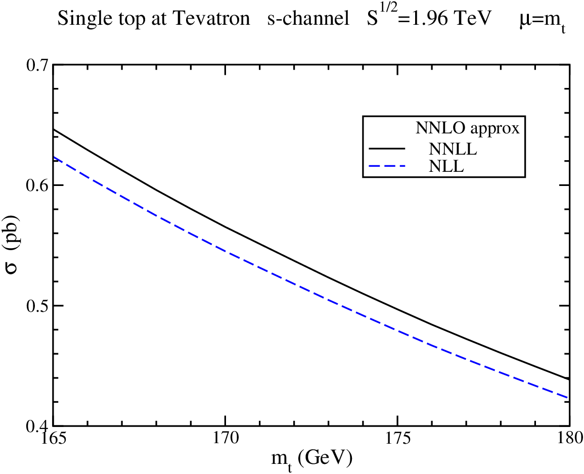
In Fig. 5 we plot the NNLO approximate cross section for $s$-channel single top quark production at the Fermilab Tevatron as a function of top quark mass in the range 165 GeV $\leq m_{t}\leq$ 180 GeV. The factorization and renormalization scales are set equal to each other and this common scale, denoted by $\mu$, is set equal to the top quark mass. Results are shown for the NNLO expansion from both NLL and NNLL resummation. The NLL result uses the expressions in [7] while the NNLL result uses the new expression in Eq. (). It is clear that the approximate NNLO cross section is larger at NNLL than at NLL, i.e. the additional NNLL numerical contributions are positive.

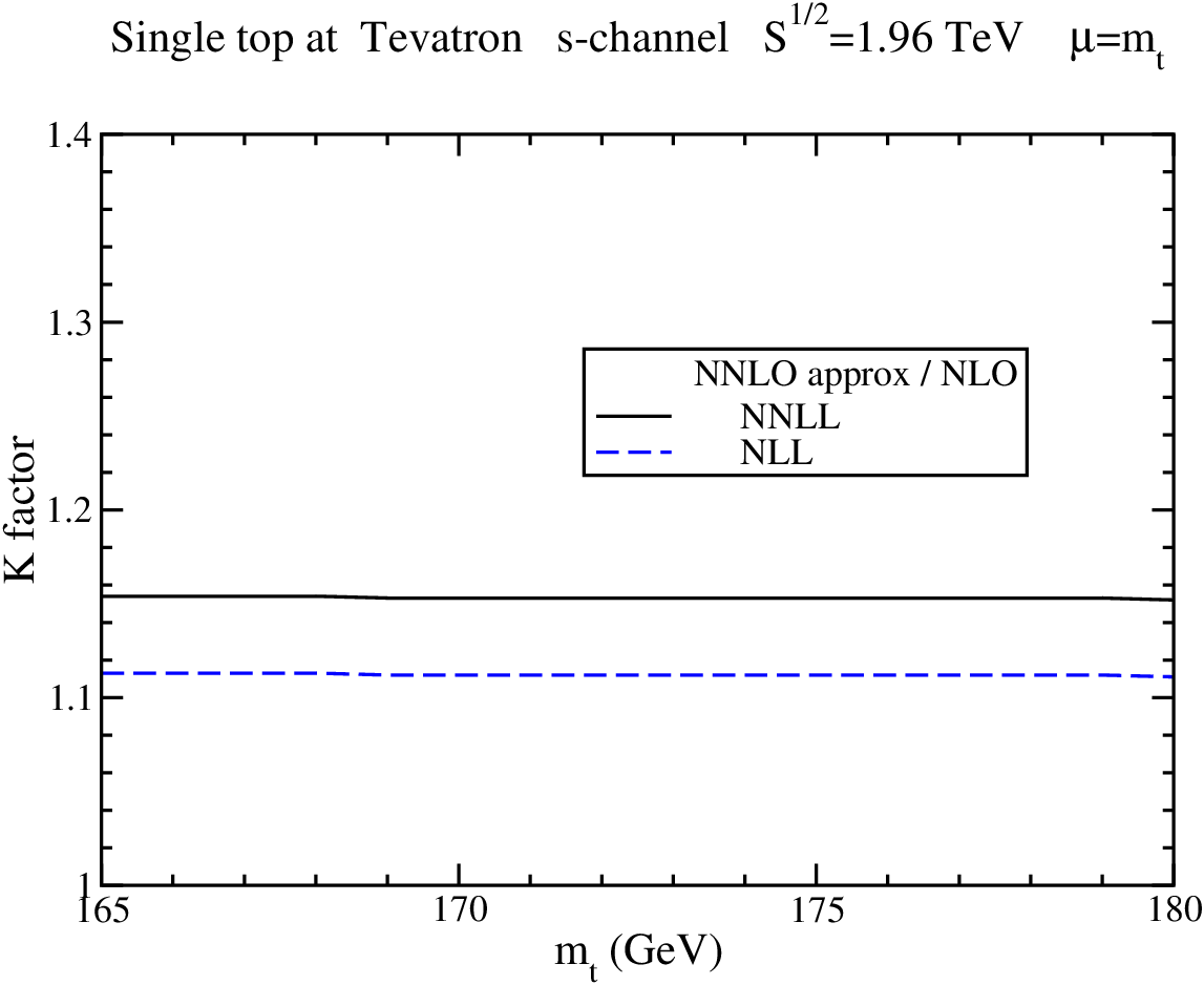
It is important to know the additional contribution of the NNLO soft-gluon corrections at both NLL and NNLL accuracy relative to the NLO cross section. The corresponding $K$ factors, defined as the ratio of the NNLO approximate cross section to the NLO cross section, are displayed in Fig. 6. It is clear that the $K$ factors are quite insensitive to the value of the top quark mass. At NLL there is an 11% enhancement over NLO, while at NNLL there is a 15% enhancement over NLO. Thus the enhancement from soft-gluon corrections is quite significant at both NLL and NNLL accuracy. Also the new NNLL contributions increase the approximate NNLO cross section of NLL accuracy by an additional 3.7%.

Table 1 lists the values of the approximate NNLO cross section at NNLL accuracy for top quark masses between 170 GeV and 175 GeV and with $\mu=m_{t}$. There are theoretical uncertainties associated with these values that arise from the dependence on the scale $\mu$ as well as from pdf errors. The scale uncertainty is most commonly estimated by varying the scale by a factor of two, i.e. between $m_{t}/2$ and $2m_{t}$. For the approximate NNLO cross section at NNLL at the Tevatron the scale uncertainty is +0.1% $-$1.0%, which is a significant improvement over NLO [5, 6] as well as over the NLL approximation [7]. The pdf uncertainty is calculated using the 40 different MSTW2008 NNLO eigensets as provided by MSTW at 90% confidence level (C.L.) [22] which provides a conservative estimate of pdf error. For $s$-channel single top quark production at the Tevatron this 90% C.L. pdf uncertainty is +5.7% $-$5.3%. If instead one uses the 68% C.L. NNLO eigensets provided by MSTW, the pdf uncertainty of the cross section becomes considerably smaller, +2.7% $-$2.4%, but it is still larger than the scale uncertainty. Clearly at Tevatron energies the pdf uncertainty dominates the theoretical uncertainty in our approximate NNLO cross section at NNLL whether one uses the conservative 90% C.L. or the 68% C.L. pdf eigensets.

The best current value of the top quark mass is $173$ GeV [23]. For this top quark mass we write the cross section and its associated uncertainties expilicitly as

$$\sigma_{\rm s-ch}^{\rm top}(m_{t}=173\,{\rm GeV},\,\sqrt{S}=1.96\,{\rm TeV})=0.523^{+0.001}_{-0.005}{}^{+0.030}_{-0.028}\;{\rm pb}$$

(3.1)

where the first uncertainty is from scale variation and the second is the pdf uncertainty at 90% C.L.

We continue with numerical results for $s$-channel single top quark production at the LHC. We present results for three different energies: the design energy of 14 TeV, the planned starting energy of 7 TeV, and a possible intermediate run at 10 TeV. Again we use the MSTW2008 NNLO pdf [22]. We note that at the LHC the single top and single antitop cross sections are different. In this section we focus on single top production, and we discuss single antitop production in the following section.

In Fig. 7 we plot the NNLO approximate cross section for $s$-channel single top quark production at the LHC at its design energy of $\sqrt{S}=14$ TeV as a function of top quark mass. Results are shown for the NNLO expansion from both NLL and NNLL resummation. The NNLL result is larger than the NLL one.

The $K$ factor, i.e. the ratio of the NNLO approximate cross section to the NLO cross section, is displayed in Fig. 8 at both NLL and NNLL. Again the $K$ factors are quite insensitive to the value of the top quark mass. At NLL there is nearly a 10% enhancement over NLO, while at NNLL there is a 13% enhancement over NLO. The enhancement from soft-gluon corrections is similar to that for Tevatron collisions and is again quite significant at both NLL and NNLL accuracy.

Table 1 lists the NNLO approximate cross section at NNLL accuracy for top quark masses between 170 GeV and 175 GeV for $\mu=m_{t}$ at 14 TeV. The scale uncertainty of the results is $\pm 1.8$% and the pdf uncertainty at 90% C.L. is +3.9% $-$3.5%, which is about twice as big as the scale uncertainty, while at 68% C.L. it is +2.0% $-$2.2%. For a top quark mass of 173 GeV the explicit result is

$$\sigma_{\rm s-ch}^{\rm top}(m_{t}=173\,{\rm GeV},\,\sqrt{S}=14\,{\rm TeV})=7.93\pm 0.14{}^{+0.31}_{-0.28}\;{\rm pb}$$

(4.1)

where the first uncertainty is from scale variation and the second is from the pdf error at 90% C.L.

Fig. 9 shows the NNLO approximate cross section at NNLL accuracy for $s$-channel single top quark production at the LHC at the starting energy of $\sqrt{S}=7$ TeV and also at 10 TeV and at 14 TeV. The enhancement over NLO at 7 TeV and 10 TeV is very similar to that at 14 TeV, over 13%.

Results for the cross section with $\mu=m_{t}$ at 10 TeV and 7 TeV are also displayed in Table 1. At 10 TeV the scale uncertainty of the results is $\pm 1.8$% while the pdf uncertainty at 90% C.L. is +3.9% $-$2.8% and at 68% C.L. it is +2.2% $-$1.4%. For a top mass of 173 GeV we have

$$\sigma_{\rm s-ch}^{\rm top}(m_{t}=173\,{\rm GeV},\,\sqrt{S}=10\,{\rm TeV})=5.16\pm 0.09{}^{+0.20}_{-0.14}\;{\rm pb}$$

(4.2)

where the first uncertainty is from scale variation and the second from the pdf at 90% C.L.

At 7 TeV the scale uncertainty is $\pm 1.9$% while the pdf uncertainty is +4.2% $-$3.1% at 90% C.L. and +2.2% $-$1.6% at 68% C.L. For $m_{t}=173$ GeV we have

$$\sigma_{\rm s-ch}^{\rm top}(m_{t}=173\,{\rm GeV},\,\sqrt{S}=7\,{\rm TeV})=3.17\pm 0.06{}^{+0.13}_{-0.10}\;{\rm pb}$$

(4.3)

where the first uncertainty is from scale variation and the second from the pdf at 90% C.L.

The dependence of the NNLO approximate cross section at NNLL accuracy on the LHC energy is plotted in Fig. 10 for the range $2\leq\sqrt{S}\leq 14$ TeV with $m_{t}=173$ GeV. We see that the cross section at 14 TeV is about twenty four times bigger than at 2 TeV.

We continue with results for single antitop production at the LHC in the $s$ channel.

Fig. 11 shows the NNLO approximate cross section at NNLL accuracy for $s$-channel single antitop production at the LHC for energies of 7 TeV, 10 TeV, and 14 TeV, using the MSTW2008 NNLO pdf [22]. The cross sections are smaller than the corresponding ones for single top quark production by a factor of around two.

Table 2 lists the values of the single antitop approximate NNLO cross section at NNLL accuracy in the $s$-channel for antitop masses between 170 GeV and 175 GeV and $\mu=m_{t}$ for the three LHC energies.

At 14 TeV the scale uncertainty is $\pm 1.3$%. The pdf uncertainty is +3.4% $-$5.2% at 90% C.L. and +1.7% $-$3.4% at 68% C.L. For $m_{t}=173$ GeV, we find

$$\sigma_{\rm s-ch}^{\rm antitop}(m_{t}=173\,{\rm GeV},\,\sqrt{S}=14\,{\rm TeV})=3.99\pm 0.05{}^{+0.14}_{-0.21}\;{\rm pb}$$

(5.1)

where the first uncertainty is from scale variation and the second from the pdf at 90% C.L.

At 10 TeV the scale uncertainty is $\pm 0.9$% while the pdf uncertainty is +3.5% $-$5.3% at 90% C.L. and +1.5% $-$3.3% at 68% C.L. For $m_{t}=173$ GeV, we find

$$\sigma_{\rm s-ch}^{\rm antitop}(m_{t}=173\,{\rm GeV},\,\sqrt{S}=10\,{\rm TeV})=2.48\pm 0.02{}^{+0.09}_{-0.13}\;{\rm pb}$$

(5.2)

where the first uncertainty is from scale variation and the second from the pdf at 90% C.L.

At 7 TeV the scale uncertainty is $\pm 0.7$%, and the pdf uncertainty is +4.2% -5.0% at 90% C.L. and +1.9% $-$2.6% at 68% C.L. For $m_{t}=173$ GeV, we find

$$\sigma_{\rm s-ch}^{\rm antitop}(m_{t}=173\,{\rm GeV},\,\sqrt{S}=7\,{\rm TeV})=1.42\pm 0.01{}^{+0.06}_{-0.07}\;{\rm pb}$$

(5.3)

where the first uncertainty is from scale variation and the second from the pdf at 90% C.L.

The dependence of the NNLO approximate cross section at NNLL accuracy for single antitop production on the LHC energy is plotted in Fig. 12 for the range $2\leq\sqrt{S}\leq 14$ TeV and $m_{t}=173$ GeV.

The single top quark production cross section in the $s$-channel receives significant contributions from soft-gluon corrections which increase the overall cross section and decrease the scale dependence of the theoretical prediction. The resummation of these corrections was performed at NNLL accuracy in this paper using an explicit calculation of the two-loop soft anomalous dimension. Approximate NNLO cross sections, which include NNLO soft-gluon corrections added to the NLO result, were calculated. Detailed numerical results were presented for single top and single antitop production at the Tevatron and the LHC. The enhancement at the Tevatron over NLO is 15% and at the LHC it is 13%. In addition to the scale uncertainty, the pdf uncertainty was calculated using 90% C.L. and 68% C.L. eigensets. At 90% C.L. the pdf uncertainty clearly dominates the theoretical error at both Tevatron and LHC energies. The overall theoretical uncertainty of the approximate NNLO cross section from NNLL resummation is reduced compared to that at NLO or at NLL accuracy.

This work was supported by the National Science Foundation under Grant No. PHY 0855421.

References

- [1] D0 Collaboration, V.M. Abazov et al., Phys. Rev. Lett. 103, 092001 (2009), arXiv:0903.0850 [hep-ex]; Phys. Lett. B 682, 363 (2010), arXiv:0907.4259 [hep-ex]; arXiv:0912.1066 [hep-ex].
- [2] CDF Collaboration, T. Aaltonen et al., Phys. Rev. Lett. 103, 092002 (2009), arXiv:0903.0885 [hep-ex].
- [3] E. Palencia, 0905.4279 [hep-ex]; D. Gillberg, 0906.0523 [hep-ex]; Tevatron Electroweak Working Group, 0908.2171 [hep-ex]; R. Schwienhorst, 0908.4553 [hep-ex]; A.P. Heinson, 0909.4518 [hep-ex]; C.E. Gerber, 0909.4794 [hep-ex]; L. Li, 0911.1150 [hep-ex].
- [4] W. Wagner, Rept. Prog. Phys. 68, 2409 (2005) [hep-ph/0507207]; A. Quadt, Eur. Phys. J. C 48, 835 (2006); R. Kehoe, M. Narain, and A. Kumar, Int. J. Mod. Phys. A 23, 353 (2008), arXiv:0712.2733 [hep-ex]; T. Han, Int. J. Mod. Phys. A 23, 4107 (2008), arXiv:0804.3178 [hep-ph]; W. Bernreuther, J. Phys. G 35, 083001 (2008), arXiv:0805.1333 [hep-ph]; D. Wackeroth, 0810.4176 [hep-ph]; M.-A. Pleier, Int. J. Mod. Phys. A 24, 2899 (2009), 0810.5226 [hep-ex]; J.R. Incandela, A. Quadt, W. Wagner, and D. Wicke, Prog. Part. Nucl. Phys. 63, 239 (2009), 0904.2499 [hep-ex].
- [5] B.W. Harris, E. Laenen, L. Phaf, Z. Sullivan, and S. Weinzierl, Phys. Rev. D 66, 054024 (2002) [hep-ph/0207055].
- [6] Q.-H. Cao, R. Schwienhorst, and C.-P. Yuan, Phys. Rev. D 71, 054023 (2005) [hep-ph/0409040]; S. Heim, Q.-H. Cao, R. Schwienhorst, and C.-P. Yuan, 0911.0620 [hep-ph].
- [7] N. Kidonakis, Phys. Rev. D 74, 114012 (2006) [hep-ph/0609287].
- [8] N. Kidonakis, Phys. Rev. D 75, 071501(R) (2007) [hep-ph/0701080].
- [9] N. Kidonakis, Acta Phys. Polon. B 39, 1593 (2008), arXiv:0802.3381 [hep-ph]; Nucl. Phys. A 827, 448c (2009), arXiv:0901.2155 [hep-ph]; in DPF 2009, arXiv:0909.0037 [hep-ph].
- [10] N. Kidonakis, Phys. Rev. Lett. 102, 232003 (2009), arXiv:0903.2561 [hep-ph].
- [11] N. Kidonakis, in DPF 2009, arXiv:0910.0473 [hep-ph].
- [12] N. Kidonakis and G. Sterman, Phys. Lett. B 387, 867 (1996); Nucl. Phys. B 505, 321 (1997) [hep-ph/9705234]; N. Kidonakis, G. Oderda, and G. Sterman, Nucl. Phys. B 531, 365 (1998) [hep-ph/9803241].
- [13] N. Kidonakis, Mod. Phys. Lett. A 19, 405 (2004) [hep-ph/0401147]; Phys. Rev. D 73, 034001 (2006) [hep-ph/0509079].
- [14] G. Sterman, Nucl. Phys. B 281, 310 (1987).
- [15] S. Catani and L. Trentadue, Nucl. Phys. B 327, 323 (1989).
- [16] J. Kodaira and L. Trentadue, Phys. Lett. 112B, 66 (1982).
- [17] H. Contopanagos, E. Laenen, and G. Sterman, Nucl. Phys. B 484, 303 (1997) [hep-ph/9604313].
- [18] N. Kidonakis and V. Del Duca, Phys. Lett. B 480, 87 (2000) [hep-ph/9911460].
- [19] S.M. Aybat, L.J. Dixon, and G. Sterman, Phys. Rev. D 74, 074004 (2006) [hep-ph/0607309].
- [20] N. Kidonakis and R. Vogt, Phys. Rev. D 68, 114014 (2003) [hep-ph/0308222]; Phys. Rev. D 78, 074005 (2008), arXiv:0805.3844 [hep-ph].
- [21] N. Kidonakis, Phys. Rev. D 77, 053008 (2008), arXiv:0711.0142 [hep-ph].
- [22] A.D. Martin, W.J. Stirling, R.S. Thorne, and G. Watt, Eur. Phys. J. C 63, 189 (2009), arXiv:0901.0002 [hep-ph].
- [23] Tevatron Electroweak Working Group, arXiv:0903.2503 [hep-ex].