Ghost anomalous dimension in asymptotically safe quantum gravity

The asymptotic-safety scenario, introduced by Weinberg in 1979 [1, 2, 3], provides for a promising route to a fully consistent and predictive theory of quantum gravity. Purely within the framework of standard local quantum field theory, gravity can become renormalizable at an interacting non-Gaußian fixed point in the ultraviolet (UV). A verification of this scenario requires a non-perturbative analysis of the renormalization flow induced by the fluctuations of the gravitational degrees of freedom of the theory.

Convincing evidence for this scenario has been collected in the past years, using the metric field itself as the microscopic degree of freedom. Based on the pioneering work of Reuter [4], the renormalization flow of generic gravitational theories including Einstein-Hilbert terms and higher-order curvature invariants has been studied within the functional RG [5, 6, 7, 10, 8, 9, 11, 12, 13, 14, 15, 16, 17, 23, 18, 19, 20, 25, 21, 22, 26, 24, 27] and other field-theoretical methods [28, 29]. These results do not only agree on the existence of a non-Gaußian fixed point, but also on the classification of renormalization group (RG) relevant and irrelevant directions. In particular, the number of RG relevant directions corresponds to the number of physical parameters to be fixed for the theory to be fully predictive; there are strong indications from high-order calculations that this number is finite [23, 25, 24], lending substantial support to the scenario that Quantum Einstein Gravity (QEG) is asymptotically safe and applicable to diverse physical scenarios. For instance, the implications of QEG for cosmology as well as black hole physics have been studied in [30, 31, 32]. Some features of the asymptotic-safety scenario are also reminiscent to results obtained within other nonperturbative approaches to a quantum field theory of gravity [33, 34, 35, 36].

The concept of asymptotic safety, of course, extends to general quantum field theories: for instance, corresponding scenarios curing the triviality problem of the Higgs sector of the particle-physics standard model have been developed in the pure matter sector [37, 38] and also including gravity [39, 40].

As for any quantum field theory with a local symmetry group, a continuum formulation based on the gauge-variant degrees of freedom requires gauge fixing conventionally accompanied by Faddeev-Popov ghosts. Whereas most studies have concentrated on gauge-invariant building blocks of the theory, the investigation of the renormalization flow of the ghost sector has started only recently [41]. Even though the ghosts do not belong to the physical state space, their fluctuations can, in principle, contribute in an important manner to gauge-invariant observables, depending on the details of the gauge. In fact, in the Landau gauge in Yang-Mills theory, the ghost sector can even carry crucial physical information in the strongly interacting regime of the theory, as is, for instance, expressed in the Kugo-Ojima or Gribov-Zwanziger scenarios for confinement: here, signatures for the physical property of confined color charges occur in the form of a strongly divergent ghost propagator in the infrared, whereas the gluon propagator is finite or even zero [42, 43, 44, 45, 46]. These properties can be related to the existence of Gribov copies, i.e., the non-uniqueness of the gauge-fixing condition and the related zeros of the Faddeev-Popov operator [43, 44]. This problem also exists in gravity [47, 48], where it is even more challenging due to the highly non-trivial topology of the diffeomorphism group.

As an indicator for the relevance of ghost fluctuations at a UV fixed point of asymptotically safe Quantum Gravity, we compute the ghost anomalous dimension in this work. On the one hand this measures how these gauge-variant degrees of freedom propagate in a given gauge, on the other hand the ghost backreaction on the renormalization flow of the graviton sector provides for another nontrivial test of the existence of the UV fixed point.

Such investigations require a non-perturbative tool which supports an approach to quantum gravity within systematic and consistent approximation schemes. Such an advanced framework is provided by the functional renormalization group which facilitates studies not only of a given action but of the renormalization flow of generic effective actions in theory space (for reviews for gauge theories, see [49]). The functional RG can be formulated in terms of a flow equation for a scale-dependent effective average action $\Gamma_{k}$ with $k$ denoting a momentum scale. The Wetterich flow equation [50] relates the flow of $\Gamma_{k}$ to the trace of the full non-perturbative propagator,

where $t=\ln k$ and $\Gamma_{k}^{(2)}$ denotes the second functional derivative with respect to the fields. The regulator function $R_{k}$ acts as a momentum- and $k$-dependent mass term and cuts off momentum modes with $p^{2}\lesssim k^{2}$. Accordingly, the limit $k\rightarrow\infty$ is related to the classical action $S_{\rm cl}$ [51], whereas the full quantum effective action $\Gamma$ is obtained for $k\rightarrow 0$.

As $\Gamma_{k}$ is a functional in the infinite dimensional space of all operators compatible with the symmetry constraints, an exact solution of the Wetterich equation is difficult. Approximate solutions can be found by truncating a systematic expansion of the effective action. The reliability of an approximation can be studied not only by checking its internal consistency but also by actively monitoring the convergence of physical quantities at increasing order in this expansion.

In order to extract gauge-invariant parts of the action functional, the background-field formalism [52] is most convenient. Here the full metric $\gamma_{\mu\nu}$ is split into a background $\bar{g}_{\mu\nu}$ and a fluctuation metric $h_{\mu\nu}$:

Accordingly, we denote covariant derivatives compatible with the full or background metric by $D_{\mu}$ or $\bar{D}_{\mu}$, respectively. In the present work, we study the following truncation of the effective action in four dimensions:

where

with

Herein, $\bar{\kappa}=(32\pi G_{\text{N}})^{-\frac{1}{2}}$ is related to the bare Newton constant $G_{\text{N}}$. The ghost term with a wave function renormalization $Z_{c}$ is given by

In this work we neglect the possibility of a different flow for the two tensor structures in the kinetic ghost term and focus on the single wave function renormalization $Z_{c}$.

During the course of the flow, we also identify the full metric $\gamma_{\mu\nu}$ with the background metric $\bar{g}_{\mu\nu}$, once the propagator of the fluctuation field is determined. This approximation appears justified for many aspects of the Einstein-Hilbert sector [53]. More generally, we expect bimetric truncations to be mandatory for a computation of (momentum-dependent) propagators and vertices. For instance in Yang-Mills theories, the distinction between fluctuation and background is crucial for the computation of gauge-invariant infrared observables [54].

The paper is organized as follows: Sect. II summarizes our method to extract the ghost anomalous dimension and presents general results for a class of covariant gauges and a spectrally adjusted regulator. In Sect. III, explicit results for the Landau-deWitt gauge and the deDonder gauge are given. We discuss the implications of our results and conclude in Sect. IV. Many technical details and explicit representations may be found in the appendices.

In order to extract the anomalous dimension of the ghost, we project the flow equation onto the running of the ghost wave function renormalization. We use a decomposition of $\Gamma^{(2)}_{k}+R_{k}=\mathcal{P}+\mathcal{F}$ into an inverse propagator matrix $\mathcal{P}=\Gamma_{k}^{(2)}[\bar{c}=0=c]+R_{k}$, including the regulator but no external ghost fields, and a fluctuation matrix $\mathcal{F}=\Gamma_{k}^{(2)}[\bar{c},c]-\Gamma_{k}^{(2)}[\bar{c}=0=c]$ containing external ghost fields. The components of $\mathcal{F}$ are either linear or bilinear in the ghost fields, as higher orders do not occur in our truncation. We may now expand the right-hand side of the flow equation as follows:

where the derivative $\tilde{\partial}_{t}$ in the second line by definition acts only on the $k$ dependence of the regulator, $\tilde{\partial}_{t}=\int\partial_{t}R_{k}\frac{\delta}{\delta R_{k}}$. Since each factor of $\mathcal{F}$ contains a coupling to external fields, this expansion simply corresponds to an expansion in the number of vertices.

To bilinear order in the external ghost and antighost, we may directly neglect all contributions beyond $(\mathcal{P}^{-1}\mathcal{F})^{2}$. Diagrammatically, the remaining terms correspond to a tadpole and a self-energy diagram.

Irrespective of our choice of gauge in the ghost sector, i.e., for all values of the gauge parameter $\rho$, we find that the tadpole does not contribute to the ghost anomalous dimension as the corresponding vertex is zero; this is shown in appendix A.

We take advantage of the possibility to specify a concrete background for computational purposes in order to project unambiguously onto the running couplings. For the running of the ghost wave function renormalization, it suffices to choose a flat background, i.e. $\bar{g}_{\mu\nu}=\delta_{\mu\nu}$, as this allows for a clean separation between the kinetic ghost operator and higher-order operators coupling ghost bilinears to curvature invariants. It is important to stress that this choice of background has nothing to do with a perturbative reasoning, where one would consider small metric fluctuations around a flat background. For the projection of the Wetterich equation, any convenient background that helps distinguishing different operators unambiguously can be used in order to extract the corresponding $\beta$ functions. In fact, we are allowed to choose different backgrounds for extracting the flow of different operators. The notion of a background in the sense of the true quantum expectation value of the field can finally be computed, once the full effective action is known.

On a flat background, we project the flow equation in Fourier space onto the running wave function renormalization by

Our conventions for the functional Grassmannian derivatives are such that

where $\delta(p,q)=(2\pi)^{4}\delta^{(4)}(p-q)$. In the following, we decompose the fluctuation metric into irreducible representations of the Poincaré group in momentum space, i.e., transverse traceless ($h^{\text{T}}_{\mu\nu}$), transverse vector ($v_{\mu}$), and scalar ($\sigma$ and $h$) degrees of freedom:

where $h(p)=\gamma^{\mu\nu}h_{\mu\nu}$ is the conformal mode. In this decomposition of the graviton, the quantities $\mathcal{P}^{-1}$ and $\mathcal{F}$ are $6\times 6$ matrices in field space $\phi=(h^{\text{T}}_{\mu\nu},v_{\mu},\sigma,h,\bar{c}_{\mu},c_{\mu})$. In the following, we confine ourselves to the gauge choice $\rho\rightarrow\alpha$ for which the propagator matrix is diagonal in the graviton modes and off-diagonal in the ghosts. Accordingly, the product $\left(\mathcal{P}^{-1}\mathcal{F}\right)^{2}$ decomposes into four terms from the four different graviton modes, which may be considered separately. The corresponding matrix elements of $\mathcal{P}^{-1}$ and $\mathcal{F}$ which build up the self-energy diagram can be decomposed into elementary propagators and vertices for these modes, listed in detail in appendix B. Incidentally, the gauge choice $\rho\to\alpha$ becomes problematic for $\rho=\alpha=3$: here, both the inverse ghost as well as the inverse scalar graviton propagators develop a zero mode. The inverse propagator is thus not invertible, signaling that the gauge fixing is no longer complete for this choice. Nevertheless, the most important standard gauge choices $\alpha=0$ or $\alpha=1$ are unaffected by this problem.

The matrix multiplication in Eq. (8) to second order in the vertices can be performed straightforwardly. Also, the trace over Lorentz indices and momentum variables can efficiently be performed by standard means and simplifies by using the projection rule as specified by Eq. (9). Finally evaluating the $\tilde{\partial}_{t}$ derivative necessitates a more explicit form of the regulator. We choose a spectrally and RG-adjusted regulator [55, 56],

Herein, the wave function renormalization $Z$ in the regulator is adapted to each mode, such that the cutoff scales for each mode are equal; this implies that the factor of $Z$ also contains the numerical prefactors from Eq. (35) for the transverse, vector, scalar and conformal mode. This adjustment is useful, as different effective cutoff scales for different modes could artificially alter the results within a truncation.

We thereby arrive at the following flow equation, where the first line is the transverse traceless contribution. The second line is due to the transverse vector mode, and the last two lines result from the two scalar modes, respectively. The terms $\sim r^{\prime}$ are due to the external momentum $\tilde{p}$ flowing through the internal ghost line and being acted upon by the $\partial_{\tilde{p}^{2}}$-derivative in Eq. (9).

The Landau-deWitt gauge $\alpha=0$ clearly plays a distinguished role as only the transverse traceless and the conformal mode propagate. This feature appears generically in all diagrams with more than one vertex as the propagator is $\sim\alpha$. This favors the Landau-deWitt gauge from a computational point of view. As it is moreover a fixed point of the renormalization group flow [57, 58], we consider the Landau-deWitt gauge as our preferred gauge choice.

For explicit computations, we use an exponential regulator shape function $r(y)$,

Such a smooth shape function is advantageous here as the evaluation of $\eta_{\text{N}}=-\partial_{t}\ln Z_{\text{N}}$ and $\partial_{t}\lambda$ require up to second-order derivatives.
Introducing the dimensionless Newton coupling and cosmological constant,

we arrive at an explicit form for the ghost anomalous dimension, which is given in appendix D for the Landau-deWitt ($\alpha=0$) and the deDonder ($\alpha=1$) gauge.

Endowing the ghost propagator with a non-trivial wave function renormalization $\eta_{c}$ feeds back into the flow equations in the Einstein-Hilbert sector by virtue of the ghost loop. We evaluate the graviton anomalous dimension $\eta_{\text{N}}$ and the flow of the cosmological constant $\partial_{t}\lambda$ by expanding the propagators in a basis of tensor, vector and scalar hyperspherical harmonics on a $d$ sphere and find the $\beta$ functions given in Appendix C.
This flow of the Einstein-Hilbert sector has been analyzed in a variety of computations in the literature, e.g. [4, 6, 18, 9, 13, 20]. From a technical viewpoint, our computational method differs from the literature as we do not rely on heat-kernel results. Apart from this minor detail, our results are in perfect agreement with the literature; in particular, our choice of a spectrally adjusted regulator corresponds to type III in [18]. The new modifications arising from the flow of the ghost sector correspond to the additional terms $\propto\eta_{c}$.

For the UV fixed-point search, we insert the expression for $\eta_{c}$ into Eq. (40) and Eq. (39). Imposing the fixed-point condition $\eta_{\text{N}}=-2$ and $\partial_{t}\lambda=0$, we then find the fixed point values and eigenvalues $\theta_{1,2}$ of the stability matrix, which may be compared to their counterparts in a truncation where $\eta_{c}=0$:

The gauge dependences for the fixed-point values $\lambda_{\ast}$ and $G_{\ast}$ agree with those found e.g. in [8] for different regulators. The value of the ghost anomalous dimension also exhibits a sizable gauge dependence. Our results provide evidence that $\eta_{c}<0$ is valid for all admissible choices of $\alpha$ with a maximum value of $\eta_{c,\text{ max}}=-0.778944$ being acquired in the Landau-deWitt gauge in the present truncation. This is due to the fact that the conformal mode contributes with a positive sign to $\eta_{c}$ (for $G_{\ast}>0$), whereas the other modes typically contribute with a negative sign. As the scalar and the vector contribution are both proportional to $\alpha$, $\eta_{c}$ decreases with increasing $\alpha$.

Another important observation is that the inclusion of the ghost anomalous dimension on average leads to a weaker gauge dependence in the Einstein-Hilbert sector, as might be read off from table III. This can be taken as a signature for the convergence of the expansion of the effective action.

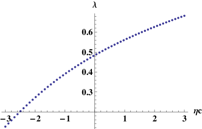
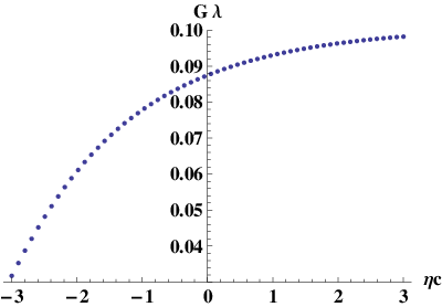
We observe a rather strong dependence of the cosmological-constant fixed point $\lambda_{\ast}$ on the ghost anomalous dimension, whereas $G_{\ast}$ shows only a mild variation. In order to test the stability of the non-Gaußian fixed point in the Einstein-Hilbert sector against further variations of the ghost sector, let us study the $\eta_{c}$ dependence of the fixed point from a more general viewpoint. For this, we consider $\eta_{c}$ as a free parameter for the moment, and then solve the fixed-point equations for $G$ and $\lambda$ as well as the corresponding critical exponents as a function of $\eta_{c}$. This can mimic the influence of higher-order ghost operators on the true value of $\eta_{c}$.

For any $\eta_{c}\in[-3,3]$, which we expect to cover the physically relevant range, we find a physically reasonable fixed point which provides further evidence for the stability of the asymptotic-safety scenario. Quantitatively, the cosmological constant gets significantly reduced for decreasing ghost anomalous dimension. The values of $G_{\ast}$ show the opposite behavior, but much less pronounced. The universal product $G_{\ast}\lambda_{\ast}$ becomes less sensitive to $\eta_{c}$ for positive $\eta_{c}$.

Furthermore, let us investigate the “TT approximation”, where all graviton modes except for the transverse traceless mode are not allowed to propagate. This approximation has effectively been adopted in the study of the ghost-curvature coupling in [41]. As on the one hand the transverse traceless mode is the genuine spin-2 mode characteristic for gravity, and on the other hand the TT approximation is technically much easier to deal with, it is interesting to see whether this ”transverse traceless approximation” is able to capture the essential physics, such as the existence of the fixed point and the number of relevant directions. In the TT approximation and in the Landau-deWitt gauge, we find a fixed point with a negative value of $\lambda$ and a positive $G$. As there are RG trajectories where the negative cosmological constant is acquired only in the UV, this fixed point is physically admissible. The critical exponents in this approximation no longer form a complex conjugate pair of eigenvalues in the Einstein-Hilbert sector, but two positive real eigenvalues $\theta_{1}=2.808,\,\theta_{2}=1.075$. The ghost anomalous dimension is given by $\eta_{c}=-0.5515$. We conclude that the existence of the non-Gaußian fixed point as well as the number of relevant directions is correctly reproduced in the TT approximation. It is an interesting open question whether this feature of the transverse traceless approximation is generic and can be confirmed also in other truncations.

As another approximation of our full result, we can take the perturbative limit, i.e., consider the leading contribution in $G$ to $\eta_{c}$. For vanishing cosmological constant, but arbitrary gauge parameter $\alpha$ ($=\rho$), we find

Again, we observe that $\eta_{c}$ is negative for all admissible gauge parameters $\alpha\geq 0$, with a singularity at $\alpha=3$ due to incomplete gauge fixing as discussed above. The Landau-deWitt-gauge limit is $\eta_{c}=-\frac{31}{9\pi}G\simeq-1.0964G$, being in the same range as at the non-Gaußian fixed point. Of course, this result is non-universal but scheme dependent in four dimensions, as the power-counting RG critical dimension is $d=2$.

Let us finally compare our findings to very recent results by Saueressig and Groh, where $\eta_{c}=-1.85$ was obtained in the deDonder gauge applying a cutoff scheme without spectral adjustment [59]. The quantitative variation is in the range familiar from typical regulator dependencies already observed in earlier calculations, see e.g. [18]. Most importantly, the qualitative pictures mutually confirm each other.

We have computed the ghost anomalous dimension in quantum gravity in various covariant gauges. Within the asymptotic-safety scenario of quantum gravity, our work represents a further extension of existing approximation schemes for the construction of renormalizable RG trajectories. Our results provide further evidence for the existence of a non-Gaußian fixed point which facilitates a UV-complete construction of quantum gravity.

Even though the ghost anomalous dimension turns out to be large, i.e., of order one, its influence on the fixed-point properties in the Einstein-Hilbert sector remains rather moderate, confirming earlier approximations that have neglected $\eta_{c}$. On the other hand, the values that $\eta_{c}$ can acquire in standard gauges indicate that ghost contributions can become important in future analyses.

The anomalous dimension $\eta_{c}$ parameterizes the scale dependence of the wave function renormalization $Z_{c}$. As the functional RG flow is local in momentum space, we can consider the scale dependence of $Z_{c}$ as an estimate for the momentum dependence of the fully dressed inverse ghost propagator:

The corresponding correlator in position space reads

As $\eta_{c}<0$ for all cases studied in this work, the propagation of ghost modes is suppressed in the UV compared to the perturbative propagator. For those gauges (e.g., $\alpha=0$ and $\alpha=1$) where $-2<\eta_{c}<0$, the dressed correlator still develops a singularity at short distances. In general, the UV behavior of higher-order diagrams involving ghosts is improved for $\eta_{c}<0$ compared to a perturbative framework.

It is interesting to compare this to the graviton anomalous dimension which is $\eta_{\text{N}}=-2$ at the fixed point, implying an even weaker UV propagation, $G_{h}(x,x^{\prime})\sim\ln|x-x^{\prime}|$ [15]. At first sight, one might expect that a complete calculation of the ghost anomalous dimension should also result in $\eta_{c}=-2$ in order to guarantee a cancellation of gauge modes and ghost modes near the fixed point. However, this cancellation could also come about for differing anomalous dimensions if this difference is balanced by a corresponding running of the vertices with ghost legs. A mechanism of this type has for instance been observed at a non-Gaußian IR fixed point in Landau-gauge Yang Mills theory [60]. On the other hand, if this difference in the propagation of ghost and graviton modes persisted (say, if the vertices did not differ much from a trivial scaling), $\eta_{c}>\eta_{\text{N}}$ would indicate a dominance of ghost modes for the RG running. This could be a signature of the dominance of field configurations near the Gribov horizon along the lines of the Gribov-Zwanziger scenario in gauge theories [43]. We emphasize that a complete discussion of this issue also requires to distinguish between the background-field anomalous dimension $\eta_{\text{N}}$ and the corresponding fluctuation-field anomalous dimension.

Another consequence of $\eta_{c}<0$ can be read off from the induced scaling of the vertices involving ghost modes. Consider a vertex with $m$ ghost and $m$ antighost legs parameterized by a coupling $\bar{g}^{(m)}$. After renormalizing the ghost fields with $Z_{c}^{1/2}$, the $\beta$ function for the renormalized coupling $g^{(m)}\sim\bar{g}^{(m)}/Z_{c}^{m}$ receives a contribution of the type

For $\eta_{c}<0$, this increases the RG relevance of this vertex in comparison to standard power-counting. A simple example is provided by the ghost-curvature coupling $\sim\bar{\zeta}\bar{c}^{\mu}Rc_{\mu}$ considered in [41] ($m=1$ in this case). In a TT approximation, the renormalized coupling has turned out to be RG relevant for $\eta_{c}=0$. This conclusion now remains unchanged, as our values $\eta_{c}<0$ even enhance the RG relevance of this operator.