Bosonic Spectral Function and The Electron-Phonon Interaction in HTSC Cuprates
Abstract
In Part I we discuss accumulating experimental evidence related to the structure and origin of the bosonic spectral function in high-temperature superconducting (HTSC) cuprates at and near optimal doping. Some global properties of , such as number and positions of peaks, are extracted by combining optics, neutron scattering, ARPES and tunnelling measurements. These methods give convincing evidence for strong electron-phonon interaction () with in cuprates near optimal doping. Here we clarify how these results are in favor of the Eliashberg-like theory for HTSC cuprates near optimal doping.
In Part II we discuss some theoretical ingredients - such as strong EPI, strong correlations - which are necessary to explain the experimental results related to the mechanism of d-wave pairing in optimally doped cuprates. These comprise the Migdal-Eliashberg theory for EPI in strongly correlated systems which give rise to the forward scattering peak. The latter is further supported by the weakly screened Madelung interaction in the ionic-metallic structure of layered cuprates. In this approach EPI is responsible for the strength of pairing while the residual Coulomb interaction (by including spin fluctuations) triggers the d-wave pairing.
Part I Experimental Evidence for Strong EPI
I Introduction
In spite of an unprecedented intensive experimental and theoretical study after the discovery of high-temperature superconductivity (HTSC) in cuprates there is, even twenty-three years after, no consensus on the pairing mechanism in these materials. At present there are two important experimental facts which are not under dispute: (1) the critical temperature in cuprates is high, with the maximum in the Hg-1223 compounds; (2) the pairing in cuprates is d-wave like, i.e. with . On the contrary there is a dispute concerning the scattering mechanism which governs normal state properties and pairing in cuprates. To this end, we stress that in the HTSC cuprates, a number of properties can be satisfactorily explained by assuming that the quasi-particle dynamics is governed by some electron-boson scattering and in the superconducting state bosonic quasi-particles are responsible for Cooper pairing. Which bosonic quasi-particles are dominating in the cuprates is the subject which will be discussed in this work. It is known that the electron-boson (phonon) scattering is well described by the Migdal-Eliashberg theory if the adiabatic parameter fulfills the condition , where is the electron-boson coupling constant, is the characteristic bosonic energy and is the electronic band width and depends on numerical approximations [1]. The important characteristic of the electron-boson scattering is the Eliashberg spectral function (or its average ) which characterizes scattering of quasi-particle from to by exchanging bosonic energy . Therefore, in systems with electron-boson scattering the knowledge of this function is of crucial importance. There are at least two approaches differing in assumed pairing bosons in the HTSC cuprates. The first one is based on the electron-phonon interaction (EPI), with the main proponents in [2], [3], [4], [5], [6], where mediating bosons are phonons and where the average spectral function is similar to the phonon density of states . Note, is not the product of two functions although sometimes one defines the function which should approximate the energy dependence of the strength of the EPI coupling. There are numerous experimental evidence in cuprates for the importance of the EPI scattering mechanism with a rather large coupling constant in the normal scattering channel , which will be discussed in detail below. In the EPI approach is extracted from tunnelling measurements in conjunction with IR optical measurements. We stress again that the Migdal-Eliashberg theory is well justified framework for EPI since in most superconductors the condition is fulfilled. The HTSC cuprates are on the borderline and it is a natural question - under which condition can high Tc be realized in the non-adiabatic limit ? The second approach [7] assumes that EPI is too weak to be responsible for high in cuprates and it is based on a phenomenological model for spin-fluctuation interaction () as the dominating scattering mechanism, i.e. it is a non-phononic mechanism. In this (phenomenological) approach the spectral function is proportional to the imaginary part of the spin susceptibility , i.e. . NMR spectroscopy and magnetic neutron scattering give evidence that in HTSC cuprates is peaked at the antiferromagnetic wave vector and this property is very favorable for d-wave pairing. The theory roots basically on the strong electronic repulsion on Cu atoms, which is usually studied by the Hubbard model or its (more popular) derivative the t-J model. Regarding the possibility to explain high Tc solely by strong correlations, as it is reviewed in [8], we stress two facts. First, at present there is no viable theory as well as experimental facts which can justify these (non-phononic) mechanisms of pairing with some exotic pairing mechanism such as RVB pairing [8], fractional statistics and anyon superconductivity, etc. Therefore we shall not discuss these, in theoretical sense, very interesting approaches. Second, the central question in these non-phononic approaches is - do models based solely on the Hubbard Hamiltonian show up superconductivity at sufficiently high critical temperatures ( ) ? Although the answer on this important question is not definitely settled there are a number of numerical studies of these models which offer rather convincing negative answers. For instance, the sign-free variational Monte Carlo algorithm in the 2D repulsive () Hubbard model gives no evidence for superconductivity with high Tc, neither the BCS- nor Berezinskii-Kosterlitz-Thouless (BKT)-like [9]. At the same time, similar calculations show that there is a strong tendency to superconductivity in the attractive () Hubbard model for the same strength of , i.e. at finite temperature in the 2D model with the BKT superconducting transition is favored. Concerning the possibility of HTSC in the model, various numerical calculations such as Monte Carlo calculations of the Drude spectral weight [10] and high temperature expansion for the pairing susceptibility [11] have shown that there is no superconductivity at temperatures characteristic for cuprates and if it exists must be rather low - few Kelvins. These numerical results tell us that the lack of high (even in BKT phase) in the repulsive () single-band Hubbard model and in the model is not only due to thermodynamical -fluctuations (which at finite T suppress and destroy superconducting phase coherence in large systems) but it is mostly due to an inherent ineffectiveness of strong correlations to produce solely high in cuprates. These numerical results signal that the simple single-band Hubbard and its derivative the t-J model are insufficient to explain solely the pairing mechanism in cuprates and some additional ingredients must be included.
Since is rather strong in cuprates, then it must be accounted for. As it will be argued in the following, the experimental support for the importance of EPI in cuprates comes from optics, tunnelling, and recent ARPES measurements [12]. It is worth mentioning that recent ARPES activity was a strong impetus for renewed experimental and theoretical studies of EPI in cuprates. However, in spite of accumulating experimental evidence for importance of EPI with , there are occasionally reports which doubt its importance in cuprates. This is the case with recent interpretation of some optical measurements in terms of SFI only [13], [14], [15] and with LDA-DFT (local density approximation-density functional theory) band structure calculations [16], [17], where both claim that EPI is negligibly small, i.e. . The inappropriateness of these calculations will be discussed in the following Sections.
The paper is organized as follows. In Part I we will mainly discuss experimental results in cuprates at and near optimal doping by giving also minimal theoretical explanations which are related to the bosonic spectral function as well to the transport spectral function and their relations to EPI. The reason that we study only cuprates at and near optimal doping is, that in these systems there are rather well defined quasi-particles - although strongly interacting, while in highly underdoped systems the superconductivity is perplexed and possibly masked by other phenomena, such as pseudogap effects, formation of small polarons, interaction with spin and (possibly charge) order parameters, pronounced inhomogeneities of the scattering centers, etc. As ARPES experiments confirm there are no polaronic effects in systems at and near optimal doping, while there are pronounced polaronic effects due to EPI in undoped and very underdoped HTSC [5], [6]. In this work we consider mainly those direct one-particle and two-particles probes of low energy quasi-particle excitations and scattering rates which give information on the structure of the spectral functions and in systems near optimal doping. These are angle-resolved photoemission (), various arts of tunnelling spectroscopy such as superconductor/insulator/ normal metal () junctions and break junctions, scanning-tunnelling microscope spectroscopy (), infrared () and Raman optics, inelastic neutron and x-ray scattering, etc. We shall argue that these direct probes give evidence for a rather strong EPI in cuprates. Some other experiments on EPI are also discussed in order to complete the arguments for the importance of EPI in cuprates. The detailed contents of Part I is the following. In Section II we discuss some prejudices related to the strength of as well as on the Fermi-liquid behavior of HTSC cuprates. We argue that any non-phononic mechanism of pairing should have very large bare critical temperature in the presence of the large EPI coupling constant, , if the EPI spectral function is weakly momentum dependent, i.e. if like in low temperature superconductors. The fact that EPI is large in the normal state of cuprates and the condition that it must conform with d-wave pairing implies inevitably that EPI in cuprates must be strongly momentum dependent. In Section III we discuss direct and indirect experimental evidence for the importance of EPI in cuprates and for the weakness of SFI in cuprates. These are:
(A) Magnetic neutron scattering measurements - These measurements provide dynamic spin susceptibility which is in the phenomenological approach [7] related to the Eliashberg spectral function, i.e. . We stress that such an approach can be theoretically justified only in the weak coupling limit, , where is the band width and is the phenomenological SFI coupling constant. Here we discuss experimental results on YBCO which give evidence for strong rearrangement (with respect to ) of (with at and near ) by doping toward the optimal doped HTSC [18], [19]. It turns out that in the optimally doped cuprates with is drastically suppressed compared to that in slightly underdoped ones with . This fact implies that the SFI coupling constant must be small.
(B) Optical conductivity measurements - From these measurements one can extract the transport relaxation rate and indirectly an approximative shape of the transport spectral function . In the case of systems near optimal doping we discuss the following questions: (i) the physical and quantitative difference between the optical relaxation rate and the quasi-particle relaxation rate . It was shown in the past that by equating these two (unequal) quantities is dangerous and brings incorrect results concerning the quasi-particle dynamics in most metals by including HTSC cuprates too [2], [3], [20], [21], [22], [23]; (ii) methods of extraction of the transport spectral function . Although these methods give at finite temperature a blurred which is (due to the ill-defined methods) temperature dependent, it turns out that the width and the shape of the extracted are in favor of ; (iii) the restricted sum-rule for the optical weight as a function of which can be explained by strong [24], [25]; (iv) good agreement with experiments of the -dependence of the resistivity in optimally doped YBCO, where is calculated by using the spectral function from tunnelling experiments. Recent femtosecond time-resolved optical spectroscopy in which gives additional evidence for importance of EPI [26] will be shortly discussed.
(C) ARPES measurements and EPI - From these measurements the self-energy is extracted as well as some properties of . Here we discuss the following items: (i) existence of the nodal and anti-nodal kinks in optimally and slightly underdoped cuprates, as well as the structure of the ARPES self-energy () and its isotope dependence, which are all due to EPI; (ii) appearance of different slopes of at low () and high energies () which can be explained by strong EPI; (iii) formation of small polarons in the undoped HTSC was interpreted to be due to strong EPI - this gives rise to phonon side bands which are clearly seen in ARPES of undoped HTSC [6].
(D) Tunnelling spectroscopy - It is well known that this method is of an immense importance in obtaining the spectral function from tunnelling conductance. In this part we discuss the following items: (i) the extracted Eliashberg spectral function with the coupling constant from the tunnelling conductance of break-junctions in optimally doped YBCO and Bi-2212 [27]-[33] which gives that the maxima of coincide with the maxima in the phonon density of states ; (ii) existence of eleven peaks in in superconducting films [34], where these peaks match precisely with the peaks in the intensity of the existing phonon Raman scattering data [35]; (iii) the presence of the dip in dI/dV in STM which shows the pronounced oxygen isotope effect and important role of these phonons.
(E) Inelastic neutron and x-ray scattering measurements - From these experiments one can extract the phonon density of state and in some cases strengths of the quasi-particle coupling with various phonon modes. These experiments give sufficient evidence for quantitative inadequacy of LDA-DFT calculations in HTSC cuprates. Here we argue, that the large softening and broadening of the half-breathing bond-stretching phonon, of apical oxygen phonons and of oxygen buckling phonons (in LSCO, BISCO,YBCO) can not be explained by LDA-DFT. It is curious that the magnitude of the softening can be partially obtained by LDA-DFT but the calculated widths of some important modes are an order of magnitude smaller than the neutron scattering data show. This remarkable fact confirms additionally the inadequacy of LDA-DFT in strongly correlated systems and a more sophisticated many body theory for EPI is needed. The problem of EPI will be discussed in more details in Part II .
In Section IV brief summary of the Part I is given. Since we are dealing with electron-boson scattering in cuprate near optimal doping, then in Appendix A (and in Part II) we introduce the reader briefly into the Migdal-Eliashberg theory for superconductors (and normal metals) where the quasi-particle spectral function and the transport spectral function are defined.
Finally, one can pose a question - do the experimental results of the above enumerated spectroscopic methods allow a building of a satisfactory and physically reasonable microscopic theory for basic scattering and pairing mechanism in cuprates? The posed question is very modest compared with a much stringent request for the theory of everything - which would be able to explain all properties of HTSC materials. Such an ambitious project is not realized even in those low-temperature conventional superconductors where it is definitely proved that in most materials the pairing is due to EPI and many properties are well accounted for by the Migdal-Eliashberg theory. Let us mention only two examples: - First, the experimental value for the coherence peak in the microwave response at in the superconducting is much higher than the theoretical value obtained by the strong coupling Eliashberg theory [36]. So to say, the theory explains the coherence peak at in qualitatively but not quantitatively. However, the measurements at higher frequency are in agreement with the Eliashberg theory [37]. Then one can say that instead of the theory of everything we deal with a satisfactory theory, which allows us qualitative and in many aspects quantitative explanation of phenomena in superconducting state. - Second example is the experimental boron (B) isotope effect in ( ) which is much smaller than the theoretical value, i.e. , although the pairing is due solely by EPI for boron vibrations [38]. Since the theory of everything is impossible in the complex materials such as HTSC cuprates in Part I we shall not discuss those phenomena which need much more microscopic details and/or more sophisticated many-body theory. These are selected by chance: (i) large ratio which is on optimally doped YBCO and BISCO and , respectively, while in underdoped BISCO one has even ; (ii) peculiarities of the coherence peak in the microwave response in HTSC cuprates, which is peaked at much smaller than , contrary to the case of LTSC where it occurs near ; (iii) the dependence of on the number of in the unit cell; (iv) temperature dependence of the Hall coefficient; (v) distribution of states in the vortex core, etc.
The microscopic theory of the mechanism for superconducting pairing in HTSC cuprates will be discussed in Part II. In Section V we introduce an ab initio many-body theory of superconductivity which is based on the fundamental (microscopic) Hamiltonian and the many-body technique. This theory can in principle calculate measurable properties of materials such as the critical temperature , critical fields, dynamic and transport properties, etc. However, although this method is in principle exact, which needs only some fundamental constants and the chemical composition of superconducting materials, it was practically never realized in practice due to the complexity of many-body interactions - electron-electron and electron-lattice, as well as of structural properties. Fortunately, the problem can be simplified by using the fact that superconductivity is a low-energy phenomenon characterized by very small energy parameters . It turns out, that one can integrate high-energy electronic processes (which are not changed by the appearance of superconductivity) and then solve the low-energy problem by the (so called) strong-coupling Migdal-Eliashberg theory. It turns out that in such an approach the physics is separated into: (1) solving an ideal band-structure Hamiltonian with the nonlocal exact crystal potential (sometimes called excitation potential) ( - ideal band structure) which includes the static self-energy () due to high-energy electronic processes, i.e. , with , the electron-ion and Hartree potential, respectively; (2) solving the low-energy Eliashberg equations. However, the calculation of the (excited) potential and the real EPI coupling , which include high-energy many-body electronic processes - for instance large Hubbard U effects, is extremely difficult at present, especially in strongly correlated systems such as HTSC cuprates. Due to this difficulty the calculations of the EPI coupling in the past was usually based on the LDA-DFT method which will be discussed in Section VI in the contest of HTSC cuprates, where the nonlocal potential is replaced by the local potential - the ground state potential, and the real EPI coupling by the ”local” LDA one . Since the exchange-correlation effects enter via the local exchange-correlation potential it is clear that the LDA-DFT method describes strong correlations scarcely and it is inadequate in HTSC cuprates (and other strongly correlated systems such as heavy fermions) wher one needs an approach beyond the LDA-DFT method. In Section VII we discuss a minimal theoretical model for HTSC cuprates which takes into account a minimal number of electronic orbitals and strong correlations in a controllable manner [3]. This theory treats the interplay of EPI and strong correlations in systems with finite doping in a systematic and controllable way. The minimal model can be further reduced in some parameter range to the single-band model, which allows the approximative calculation of the excited potential and the non-local EPI coupling . As a result one obtains the momentum dependent EPI coupling which is for small hole-doping () strongly peaked at small transfer momenta (more precisely at ) - the forward scattering peak. In the framework of this minimal model it is possible to explain some important properties and resolve some puzzling experimental results, for instance: (a) Why is d-wave pairing realized in the presence of strong EPI? (b) Why is the transport coupling constant () rather smaller than the pairing one , i.e. ? (c) Why is the mean-field (one-body) LDA-DFT approach unable to give reliable values for the EPI coupling constant in cuprates and how many-body effects help; (d) Why is d-wave pairing robust in the presence of non-magnetic impurities and defects? (e) Why are the ARPES nodal and antinodal kinks differently renormalized in the superconducting states, etc? In spite of the encouraging successes of this minimal model, at least in a qualitative explanation of numerous important properties of HTSC cuprates, we are still at present stage far from a fully microscopic theory of HTSC cuprates which is able to explain high . In that respect at the and of Section VII we discuss possible improvements of the present minimal model in order to obtain at least a semi-quantitative theory for HTSC cuprates.
Finally, we would like to point out that in real HTSC materials there are numerous experimental evidence for nanoscale inhomogeneities. For instance recent STM experiments show rather large gap dispersion at least on the surface of BISCO crystals [39] giving rise for a pronounced inhomogeneity of the superconducting order parameter, i.e. where is the relative momentum of the Cooper pair and is the center of mass of Cooper pairs. One possible reason for the inhomogeneity of and disorder on the atomic scale can be due to extremely high doping level of in HTSC cuprates which is many orders of magnitude larger than in standard semiconductors ( vs carrier concentration). There are some claims that high is exclusively due to these inhomogeneities (of an extrinsic or intrinsic origin) which may effectively increase pairing potential [40], while some others try to explain high solely within the inhomogeneous Hubbard or model. Here we shall not discuss this interesting problem but mention only that the concept of Tc increase by inhomogeneity is ill-defined, since the increase of is defined with respect to the average value . However, is experimentally not well defined quantity and the hypothesis of an increase of by material inhomogeneities cannot be tested at all. In studying and analyzing HTSC cuprates near optimal doping we assume that basic effects are realized in nearly homogeneous systems and inhomogeneities are of secondary role, which deserve to be studied and discussed separately.
II EPI vs non-phononic mechanisms
Concerning the high in cuprates, two dilemmas have been dominating after its discovery: (i) which interaction is responsible for strong quasi-particle scattering in the normal state - this question is related also to the dilemma Fermi vs non-Fermi liquid; (ii) what is the mediating (gluing) boson responsible for the superconducting pairing, i.e. there is a dilemma phonons or non-phonons? In the last twenty-three years, the scientific community was overwhelmed by numerous proposed pairing mechanisms, most of which are hardly verifiable in HTSC cuprates.
1. Fermi vs non-Fermi liquid in cuprates
After discovery of HTSC in cuprates there was a large amount of evidence on strong scattering of quasi-particles which contradicts the canonical (popular but narrow) definition of the Fermi liquid, thus giving rise to numerous proposals of the so called non-Fermi liquids, such as Luttinger liquid, RVB theory, marginal Fermi liquid, etc. In our opinion there is no need for these radical approaches in explaining basic physics in cuprates at least in optimally, slightly underdoped and overdoped metallic and superconducting HTSC cuprates. Here we give some clarifications related to the dilemma of Fermi vs non-Fermi liquid. The definition of the canonical Fermi liquid (based on the Landau work) in interacting Fermi systems comprises the following properties: (1) there are quasi-particles with charge , spin and low-laying energy excitations which are much larger than their inverse life-times, i.e. . Since the level width of the quasi-particle is negligibly small, this means that the excited states of the Fermi liquid are placed in one-to-one correspondence with the excited states of the free Fermi gas; (2) at there is an energy level with the Fermi surface at which and the Fermi quasi-particle distribution function has finite jump at ; (3) the number of quasi-particles under the Fermi surface is equal to the total number of conduction particles (we omit here other valence and core electrons) - the Luttinger theorem; (4) the interaction between quasi-particles are characterized with a few (Landau) parameters which describe low-temperature thermodynamics and transport properties. Having this definition in mind one can say that if fermionic quasi-particles interact with some bosonic excitation, for instance with phonons, and if the coupling is sufficiently strong, then the former are not described by the canonical Fermi liquid since at energies and temperatures of the order of the characteristic (Debye) temperature (for the Debye spectrum ), i.e. for one has and the quasi-particle picture (in the sense of the Landau definition) is broken down. In that respect an electron-boson system can be classified as a non-canonical Fermi liquid for sufficiently strong electron-boson coupling. It is nowadays well known that for instance Al, Zn are weak coupling systems since for one has and they are well described by the Landau theory. However, in (the non-canonical) cases, where for higher energies one has , the electron-phonon system is satisfactory described by the Migdal-Eliashberg theory and the Boltzmann theory, where thermodynamic and transport properties depend on the spectral function and its higher momenta. Since in HTSC cuprates the electron-boson (phonon) coupling is strong and is large, i.e. of the order of characteristic boson energies (), , then it is natural that in the normal state (at ) we deal with a strong interacting non-canonical Fermi liquid which is for modest non-adiabaticity parameter described by the Migdal-Eliashberg theory, at least qualitatively and semi-quantitatively. In order to justify this statement we shall in the following elucidate some properties in more details by studying optical, ARPES, tunnelling and other experiments in HTSC oxides.
2. Is there limitation of the strength of EPI?
In spite of reach experimental evidence in favor of strong EPI in HTSC oxides there was a disproportion in the research activity (especially theoretical) in the past, since the investigation of the SFI mechanism of pairing prevailed in the literature. This trend was partly due to an incorrect statement in [41] on the possible upper limit of Tc in the phonon mechanism of pairing. Since in the past we have discussed this problem thoroughly in numerous papers - for the recent one see [42], we shall outline here the main issue and results only.
It is well known that in an electron-ion crystal, besides the attractive EPI, there is also repulsive Coulomb interaction. In case of an isotropic and homogeneous system with weak quasi-particle interaction, the effective potential in the leading approximation looks like as for two external charges () embedded in the medium with the total longitudinal dielectric function ( is the momentum and is the frequency) [43], [44], i.e.
| (1) |
In case of strong interaction between quasi-particles, the state of embedded quasi-particles changes significantly due to interaction with other quasi-particles, giving rise to . In that case depends on other (than ) response functions. However, in the case when Eq.(1) holds, i. e. when the weak-coupling limit is realized, is given by [43], [44], [45]. Here, is the EPI coupling constant, is an average phonon frequency and is the Coulomb pseudo-potential, ( is the Fermi energy). The couplings and are expressed by
| (2) |
where is the density of states at the Fermi surface and is the Fermi momentum - see more in [2]. In [41] it was claimed that lattice stability of the system with respect to the charge density wave formation implies the condition for all . If this were correct then from Eq.(2) it follows that , which limits the maximal value of Tc to the value . In typical metals and if one accepts the statement in [41] that , one obtains . The latter result, if it would be correct, means that EPI is ineffective in producing not only high-Tc superconductivity but also low-temperature superconductivity (LTS with ). However, this result is in conflict first of all with experimental results in LTSC, where in numerous systems one has and . For instance, is realized in alloy which is definitely much higher than , etc.
Moreover, the basic theory tells us that is not the response function [43], [44] (contrary to the assumption in [41]). Namely, if a small external potential is applied to the system (of electrons and ions in solids) it induces screening by charges of the medium and the total potential is given by which means that is the response function. The latter obeys the Kramers-Kronig dispersion relation which implies the following stability condition [43], [44]
| (3) |
i.e. either
| (4) |
or
| (5) |
This important theorem invalidates the restriction on the maximal value of Tc in the EPI mechanism given in [41]. We stress that the condition is not in conflict with the lattice stability at all. For instance, in inhomogeneous systems such as crystal, the total longitudinal dielectric function is matrix in the space of reciprocal lattice vectors (), i.e. , and is defined by . In dense metallic systems with one ion per cell (such as metallic hydrogen) and with the electronic dielectric function and the macroscopic total dielectric function is given by [46]
| (6) |
At the same time the energy of the longitudinal phonon is given by
| (7) |
where is the ionic plasma frequency, is the local (electric) field correction - see Ref. [46]. The right condition for lattice stability requires that , which implies that for one has . The latter condition gives automatically . Furthermore, the calculations [46] show that in the metallic hydrogen (H) crystal, for all . Note, that in metallic H the EPI coupling constant is very large, i.e and Tc may reach very large value [47]. Moreover, the analyzes of crystals with more ions per unit cell [46] gives that is more a rule than an exception - see Fig. 1. The physical reason for are local field effects described by . Whenever the local electric field acting on electrons (and ions) is different from the average electric field , i.e. , there are corrections to which may lead to .

The above analysis tells us that in real crystals can be negative in the large portion of the Brillouin zone giving rise to in Eq.(2). This means that analytic properties of the dielectric function do not limit in the phonon mechanism of pairing. This result does not mean that there is no limit on Tc at all. We mention in advance that the local field effects play important role in HTSC oxides, due to their layered structure with very unusual ionic-metallic binding, thus opening a possibility for large .
In conclusion, we point out that there are no serious theoretical and experimental arguments for ignoring EPI in HTSC cuprates. To this end it is necessary to answer several important questions which are related to experimental findings in HTSC cuprates (oxides): (1) if EPI is important for pairing in HTSC cuprates and if superconductivity is of type, how are these two facts compatible? (2) Why is the transport EPI coupling constant (entering resistivity) rather smaller than the pairing EPI coupling constant (entering Tc), i.e. why one has ? (3) If EPI is ineffective for pairing in HTSC oxides, in spite of , why it is so?
3. Is a non-phononic pairing realized in HTSC?
Regarding EPI one can pose a question - whether it contributes significantly to d-wave pairing in cuprates? Surprisingly, despite numerous experiments in favor of EPI, there is a believe that EPI is irrelevant for pairing [7]. This belief is mainly based first, on the above discussed incorrect lattice stability criterion related to the sign of , which implies small EPI and second, on the well established experimental fact that d-wave pairing is realized in cuprates [48], which is believed to be incompatible with EPI. Having in mind that EPI in HTSC at and near optimal dopimng is strong with (see below), we assume for the moment that the leading pairing mechanism in cuprates, which gives d-wave pairing, is due to some non-phononic mechanism. For instance, let us assume an exitonic mechanism due to the high energy pairing boson () and with the bare critical temperature and look for the effect of EPI on . If EPI is approximately isotropic, like in most LTSC materials, then it would be very detrimental for d-wave pairing. In the case of dominating isotropic EPI in the normal state and the exitonic-like pairing, then near the linearized Eliashberg equations have an approximative form for a weak non–phonon interaction (with the large characteristic frequency )
| (8) |
For pure d-wave pairing with the pairing potential with and one obtains and the equation for Tc - see [2]
| (9) |
Here is the di-gamma function. At temperatures near one has and the solution of Eq. (9) is approximately with , . This means that for and the bare due to the non-phononic interaction must be very large, i.e. .
Concerning other non-phononic mechanisms, such as the SFI one, the effect of EPI in the framework of Eliashberg equations was studied numerically in [49]. The latter is based on Eqs.(99-101) in Appendix A. with the kernels in the normal and superconducting channels and , respectively. Usually, the spin-fluctuation kernel is taken in the FLEX approximation [50]. The calculations [49] confirm the very detrimental effect of the isotropic (-independent) EPI on d-wave pairing due to SFI. For the bare SFI critical temperature and for the calculations give very small (renormalized) critical temperature . These results tell us that a more realistic pairing interaction must be operative in cuprates and that EPI must be strongly momentum dependent [51]. Only in that case is strong EPI conform with d-wave pairing, either as its main cause or as a supporter of a non-phononic mechanism. In Part II we shall argue that the strongly momentum dependent EPI is important scattering mechanism in cuprates providing the strength of the pairing mechanism, while the residual Coulomb interaction (by including weaker SFI) triggers it to d-wave pairing.
III Experimental evidence for strong EPI
In the following we discuss some important experiments which give evidence for strong electron-phonon interaction (EPI) in cuprates. However, before doing it, we shall discuss some indicative inelastic magnetic neutron scattering measurements (IMNS) in cuprates whose results in fact seriously doubt in the effectiveness of the phenomenological SFI mechanism of pairing which is advocated in [7], [52]. First, the experimental results related to the pronounced imaginary part of the susceptibility in the normal state at and near the AF wave vector were interpreted in a number of papers as a support for the SFI mechanism for pairing [7], [52]. Second, the existence of the so called magnetic resonance peak of (at some energies ) in the superconducting state was also interpreted in a number of papers either as the origin of superconductivity or as a mechanism strongly affecting superconducting gap at the ant-nodal point.
III.1 Magnetic neutron scattering and the spin fluctuation spectral function
a. Huge rearrangement of the SFI spectral function and little change of
Before discussing experimental results in cuprates on the imaginary part of the spin susceptibility we point out that in (phenomenological) theories based on spin fluctuation interaction (SFI) the quasi-particle self-energy ( is the Matsubara frequency and is the Nambu matrix) in the normal and superconducting state and the effective (repulsive) pairing potential (where ) are assumed in the form [7]
| (10) |
Although the form of can not be justified theoretically, except in the weak coupling limit () only, it is used in the analysis of the quasi-particle properties in the normal and superconducting state of cuprates where the spin susceptibility (spectral function) Im is strongly peaked at and near the AF wave vector . Can the pairing mechanism in HTSC cuprates be explained by such a phenomenology and what is the prise for it? The best answer is to look at the experimental results related to inelastic magnetic neutron scattering (IMNS) experiments which give . In that respect very indicative and impressive IMNS measurements on , which are done by Bourges group [18], demonstrate clearly that the normal state susceptibility (the odd part of the spin susceptibility in the bilayer system) at is strongly dependent on the hole doping as it is shown in Fig. 2.

The most pronounced result for our discussion is that by varying doping there is a huge rearrangement of in the normal state, especially in the energy (frequency) region which might be important for superconducting pairing, let say . This is clearly seen in the last two curves in Fig. 2 where this rearrangement is very pronounced, while at the same time there is only small variation of the critical temperature . It is seen in Fig. 2 that in the underdoped crystal Im and are much larger than that in the near optimally doped , i.e. one has , although the difference in the corresponding critical temperatures is very small, i.e. (in ) and (in ). This pronounced rearrangement and suppression of Im (in the normal state of YBCO) by doping toward the optimal doping but with negligible change in is strong evidence that the pairing mechanism is not the dominating one in HTSC cuprates. This insensitivity of , if interpreted in term of the coupling constant , means that the latter is small, i.e. . We stress that the explanation of high Tc in cuprates by the SFI phenomenological theory [7] assumes very large SFI coupling energy with while the frequency(energy) dependence of is extracted from the fit of the NMR relaxation rate which gives [7]. To this point, the NMR measurements (of ) give that there is an anti-correlation between the decrease of the NMR spectral function and the increase of by increasing doping toward the optimal one - see [3] and References therein. The latter result additionally disfavors the SFI model of pairing [7] since the strength of pairing interaction is little affected by SFI. Note, that if instead of taking from NMR measurements one takes it from IMNS measurements, as it was done in [53], than for the same value one obtains much smaller . For instance, by taking the experimental values for in underdoped with one obtains [53], while for . The situation is even worse if one trays to fit the resistivity with in since this fit gives . These results point to a deficiency of the SFI phenomenology (at least that based on Eq.(10)) to describe pairing in HTSC cuprates.
Having in mind the results in [53], the recent theoretical interpretation in [52] of IMNS experiments [54] and ARPES measurements [55] on the underdoped in terms of the SFI phenomenology deserve to be commented. The IMNS experiments [54] give evidence for the ”hourglass” spin excitation spectrum (in the superconducting state) for the momenta at, near and far from , which is richer than the common spectrum with magnetic resonance peaks measured at . In [52] the self-energy of electrons due to their interaction with spin excitations is calculated by using Eq. (10) with and taken from [54]. However, in order to fit the ARPES self-energy and low-energy kinks (see discussion in Section C) the authors of [52] use very large value , i.e. much larger than the one used in [53]. Such a large value of has been used earlier within the Monte Carlo simulation and the fit of the Hubbard model [56]. In our opinion this value for is unrealistically large in the case of strongly correlated systems where spin-fluctuations are governed by the effective electron exchange interaction [57]. This implies that and . Note, that this value for comes out also from the theory of strongly correlated electrons in the three-band Emery model with - for parameters see Part II Section VII.
Concerning the problem related to the rearrangement of the SFI spectral function in [18] we would like to stress, that in spite that the latter results were obtained ten years ago they are not disputed by the new IMNS measurements [19] on high quality samples of the same compound (where much longer counting times were used in order to reduce statistical errors). In fact the results in [18] are confirmed in [19] where the magnetic intensity (for at and in the broad range of ) for the optimally doped (with ) is at least three times smaller than in the underoped with . This result is again very indicative sign of the weakness of SFI since such a huge reconstruction would decrease in the optimally doped if analyzed in the framework of the phenomenological SFI theory based on Eq. (10). It also implies that due to the suppression of by increasing doping toward the optimal one a straightforward extrapolation of the theoretical approach in [52] to the explanation of in the optimally doped would require an increase of to the value even larger than , what is highly improbable.
b. Ineffectiveness of the magnetic resonance peak
A less direct argument for smallness of the SFI coupling constant, i.e. and comes from other experiments related to the magnetic resonance peak in the superconducting state, and this will be discussed next. In the superconducting state of optimally doped YBCO and BISCO, is significantly suppressed at low frequencies except near the resonance energy where a pronounced narrow peak appears - the magnetic resonance peak. We stress that there is no magnetic resonance peak in some families of HTSC cuprates, for instance in LSCO, and consequently one can question the importance of the resonance peak in the scattering processes. The experiments tell us that the relative intensity of this peak (compared to the total one) is small, i.e. - see Fig 3. In underdoped cuprates this peak is present also in the normal state as it is seen in Fig 2.

After the discovery of the resonance peak there were attempts to relate it first, to the origin of the superconducting condensation energy and second, to the kink in the energy dispersion or the peak-dimp structure in the ARPES spectral function. In order that the condensation energy is due to the magnetic resonance it is necessary that the peak intensity is small [58]. is obtained approximately by equating the condensation energy with the change of the magnetic energy in the superconducting state, i.e.
| (11) |
By taking and the realistic value , one obtains . However, such a small intensity can not be responsible for the anomalies in ARPES and optical spectra since it gives rise to small coupling constant for the interaction of holes with the resonance peak, i.e. . Such a small coupling does not affect superconductivity at all. Moreover, by studying the width of the resonance peak one can extract order of magnitude of the SFI coupling constant . Since the magnetic resonance disappears in the normal state of the optimally doped YBCO it can be qualitatively understood by assuming that its broadening scales with the resonance energy , i.e. , where the line-width is given by [58]. This condition limits the SFI coupling to . We stress that the obtained is much smaller (at least by factor three) than that assumed in the phenomenological spin-fluctuation theory [7] and [52] where and , but much larger than estimated in [58] (where ). The smallness of comes out also from the analysis of the antiferromagnetic state in underdoped metals of LSCO and YBCO [59], where the small (ordered) magnetic moment points to an itinerant antiferromagnetism with small coupling constant . The conclusion from this analysis is that in the optimally doped YBCO the sharp magnetic resonance is a consequence of the onset of superconductivity and not its cause. There is also one principal reason against the pairing due to the magnetic resonance peak at least in optimally doped cuprates. Since the intensity of the magnetic resonance near is vanishingly small, though not affecting pairing at the second order phase transition at , then if it would be solely the origin for superconductivity the phase transition at Tc would be first order, contrary to experiments. Recent ARPES experiments give evidence that the magnetic resonance cannot be related to the kinks in ARPES spectra [60], [61] - see the discussion below.
Finally, we would like to point out that the recent magnetic neutron scattering measurements on optimally-doped large-volume crystals [62], where the absolute value of is measured, are questioning the interpretation of the electronic magnetism in cuprates in terms of itinerant magnetism. This experiment shows a lack of temperature dependence of the local spin susceptibility across the superconducting transition , i.e there is only a minimal change in between and . Note, if the magnetic excitations were due to itinerant quasi-particles we should have seen dramatic changes of as a function of over the whole energy range. This -independence of strongly opposes many theoretical results in [13], [14], [15] which assume that the bosonic spectral function is proportional to that can be extracted from optic measurements. This procedure gives that is strongly -dependent contrary to the experimental results in [62] - see more in Subsection B on optical conductivity.
III.2 Optical conductivity and EPI
Optical spectroscopy gives information on optical conductivity and on two-particle excitations, from which one can indirectly extract the transport spectral function . Since this method probes bulk sample (on the skin depth), contrary to ARPES and tunnelling methods which probe tiny regions ( Å) near the sample surface, this method is indispensable. However, one should be careful not over-interpreting the experimental results since is not a directly measured quantity but it is derived from the reflectivity with the transversal dielectric tensor . Here, is the high frequency dielectric function, describes the contribution of the lattice vibrations and describes the optical (dynamical) conductivity of conduction carriers. Since is usually measured in the limited frequency interval some physical modelling for is needed in order to guess it outside this range - see more in reviews [2], [3]. This was the reason for numerous misinterpretations of optic measurements in cuprates, that will be uncover below. An illustrative example for this claim is large dispersion in the reported value of - from to , i.e. almost three orders of magnitude. However, it turns out that measurements of in conjunction with elipsometric measurements of at high frequencies allows more reliable determination of [63].
1. Transport and quasi-particle relaxation rates
The widespread misconception in studying the quasi-particle scattering in cuprates was an ad hoc assumption that the transport relaxation rate is equal to the quasi-particle relaxation rate , in spite of the well known fact that the inequality holds in a broad frequency (energy) region [20]. This (incorrect) assumption was one of the main arguments against EPI as relevant scattering mechanism in cuprates. Although we have discussed this problem several times before, we do it again due to the importance of this subject.
The dynamical conductivity consists of two parts, i.e. where describes inter-band transitions which contribute at higher than intra-band energies, while is due to intra-band transitions which are relevant at low energies . (Note, that in the measurements the frequency is usually given in , where the following conversion holds .) The experimental data for in cuprates are usually processed by the generalized (extended) Drude formula [20], [21], [22], [64],
| (12) |
which is an useful representation for systems with single band electron-boson scattering which is justified in HTSC cuprates. However, this procedure is inadequate for interpreting optical data in multi-band systems such as new high-temperature superconductors Fe-based pnictides since even in absence of the inelastic intra- and inter-band scattering the effective optic relaxation rate may be strongly frequency dependent [65]. (The usefulness of introducing the optic relaxation will be discussed below and in Appendix B.) Here, enumerates the plane axis, , and are the electronic plasma frequency, the transport (optical) scattering rate and the optical mass, respectively. Very frequently it is analyzed the quantity given by [64]
| (13) |
which is determined from the half-width of the Drude-like expression for and is independent of . In the weak coupling limit , the formula for conductivity given in Appendix B Eqs. (125-128) can be written in the form of Eq.(12) where reads [21]-[22]
| (14) |
Here is the Bose distribution function. For completeness we give also the explicit form of the transport mass see [2], [3], [20], [21], [22], .
with the Kernel where is the di-gamma function. In the presence of impurity scattering one should add to . It turns out that Eq.(14) holds within a few percents also for large . Note, that and the index enumerates all scattering bosons - phonons, spin fluctuations, etc. For comparison, the quasi-particle scattering rate is given by
| (15) |
where is the Fermi distribution function. For completeness we give also the expression for the quasi-particle effective mass
| (16) |
The term is due to the impurity scattering. By comparing Eq.(14) and Eq.(15), it is seen that and are different quantities, i.e. , where the former describes the relaxation of Bose particles (excited electron-hole pairs) while the latter one describes the relaxation of Fermi particles. This difference persists also at where one has (due to simplicity we omit in the following summation over ) [20]
| (17) |
and
| (18) |
In the case of EPI with the constant electronic density of states, the above equations give that for while (as well as ) is monotonic growing for , where is the maximal phonon frequency. So, the growing of (and ) for is ubiquitous and natural for EPI scattering and has nothing to do with some exotic scattering mechanism. This behavior is clearly seen by comparing , and which are calculated for the EPI spectral function extracted from tunnelling experiments in YBCO (with ) [27] - see Fig. 4.


The results shown in Fig. 4 clearly demonstrate the physical difference between two scattering rates and (and ). It is also seen that is even more linear function of than . From these calculations one concludes that the quasi-linearity of (and ) is not in contradiction with the EPI scattering mechanism but it is in fact a natural consequence of EPI. We stress that such behavior of and (and ), shown in Fig. 4, is in fact not exceptional for HTSC cuprates but it is generic for many metallic systems, for instance 3D metallic oxides, low temperature superconductors such as , , etc. - see more in [2], [3] and References therein.
Let us discuss briefly the experimental results for and and compare these with theoretical predictions obtained by using a single band model with extracted from the tunnelling data with the EPI coupling constant [27]. In the case of YBCO the agreement between measured and calculated is very good up to energies which confirms the importance of EPI in scattering processes. For higher energies, where a mead-infrared peak appears, it is necessary to account for inter-band transitions [2]. In optimally doped () [66] the experimental results for are explained theoretically by assuming that the EPI spectral function , where is the phononic density of states in BISCO while , and - see Fig. 5(top). The agreement is rather good. At the same time the fit of by the marginal Fermi liquid phenomenology fails as it is evident in Fig. 5(bottom).


Now we will comment the so called pronounced linear behavior of (and ) which was one of the main arguments for numerous inadequate conclusions regarding the scattering and pairing bosons and EPI. We stress again that the measured quantity is reflectivity and derived ones are , and , which are very sensitive to the value of the dielectric constant . This sensitivity is clearly demonstrated in Fig. 6 for Bi-2212 where it is seen that (and ) for is linear up to much higher than in the case .

However, in some experiments [67], [68] the extracted (and ) is linear up to very high . This means that the ion background and inter-band transitions (contained in ) are not properly taken into account since too small is assumed. The recent elipsometric measurements on YBCO [69] give the value , which gives much less spectacular linearity in the relaxation rates (and ) than it was the case immediately after the discovery of HTSC cuprates, where much smaller was assumed.
Furthermore, we would like to comment on two points concerning , , and their interrelations. First, the parametrization of with the generalized Drude formula in Eq.(12) and its relation to the transport scattering rate and the transport mass is useful if we deal with electron-boson scattering in a single band problem. In [22], [65] it is shown that of a two-band model with only elastic impurity scattering can be represented by the generalized (extended) Drude formula with and dependence of effective parameters , despite the fact that the inelastic electron-boson scattering is absent. To this end we stress that the single-band approach is justified for a number of HTSC cuprates such as LSCO, BISCO etc. Second, at the beginning we said that and are physically different quantities and it holds . In order to give the physical picture and qualitative explanation for this difference we assume that . In that case the renormalized quasi-particle frequency and the transport one - defined in Eq.(12), are related and at they are given by [20], [22]
| (19) |
(For the definition of see Appendix A.) It gives the relation between and , and , respectively
| (20) |
| (21) |
The physical meaning of Eq.(19) is the following: in optical measurements one photon with the energy is absorbed and two excited particles (electron and hole) are created above and below the Fermi surface. If the electron has energy and the hole , then they relax as quasi-particles with the renormalized frequency . Since takes values then the optical relaxation is the energy-averaged according to Eq.(19). The factor is due to the two quasi-particles - electron and hole. At finite , the generalization reads [20], [22]
| (22) |
2. Inversion of the optical data and
In principle, the transport spectral function can be extracted from (or ) only at , which follows from Eq.( 17)
| (23) |
or equivalently . However, real measurements are performed at finite (at which is rather high in HTSC cuprates) and the inversion procedure is an ill-posed problem since is the de-convolution of the inhomogeneous Fredholm integral equation of the first kind with the temperature dependent Kernel - see Eq.(14). It is known that an ill-posed mathematical problem is very sensitive to input since experimental data contain less information than one needs. This procedure can cause first, that the fine structure of gets blurred (most peaks are washed out) in the extraction procedures and second, the extracted is temperature dependent even when the true is independent. This artificial -dependence is especially pronounced in HTSC cuprates because is very high. In the context of HTSC cuprates, this problem was first studied in [21], [22] where this picture is confirmed by the following results: (1) the extracted shape of in (and other cuprates) is not unique and it is temperature dependent, i.e. at higher the peak structure is smeared and only a single peak (slightly shifted to higher ) is present. For instance, the experimental data of in YBCO were reproduced by two different spectral functions , one with single peak and the other one with three peaks structure as it is shown in Fig. 7, where all spectral functions give almost identical . The similar situation is realized in optimally doped BISCO as it is seen in Fig. 8 where again different functions reproduce very well curves for and . However, it is important to stress that the obtained width of the extracted in both compounds coincide with the width of the phonon density of states [21], [22], [70]. (2) The upper energy bound for is extracted in [21], [22] and it coincides approximately with the maximal phonon frequency in cuprates as it is seen in Figs. 7-8.


These results demonstrate the importance of EPI in cuprates [21], [22]. We point out that the width of which is extracted from the optical measurements [21], [22] coincides with the width of the quasi-particle spectral function obtained in tunnelling and ARPES spectra (which we shall discuss below), i.e. both functions are spread over the energy interval . Since in cuprates this interval coincides with the width in the phononic density of states and since the maxima of and almost coincide, this is further evidence for the importance of EPI.
To this end, we would like to comment two aspects which appear from time to time in the literature. First, in some reports [13], [14], [15] it is assumed that of cuprates can be extracted also in the superconducting state by using Eq. (23). However, Eq. (23) holds exclusively in the normal state (at ) since can be described by the generalized (extended) Drude formula in Eq. (12) only in the normal state. Such an approach does not hold in the superconducting state since the dynamical conductivity depends not only on the electron-boson scattering but also on coherence factors and on the momentum and energy dependent order parameter . In such a case it is unjustified to extract from Eq. (23). Second, if (and ) in cuprates are due to some other bosonic scattering which is pronounced up to much higher energies , this should be seen in the extracted spectral function . Such an assumption is made, for instance, in the phenomenological spin-fluctuation approach [7] where it is assumed that Im where Im is extended up to the large energy cutoff . This assumption is in conflict with the above theoretical and experimental analysis which shows that solely EPI can describe very well and that the contribution from higher energies must be small and therefore irrelevant for pairing [21], [22], [70]. The finding of the importance of EPI is also confirmed by tunnelling measurements - see discussion in Subsection D. Despite the experimentally established facts, that the energy width of the extracted coincides with the phononic range, which favor EPI, some reports appeared recently claiming that SFI dominates and that where [14], [15]. This claim is based on reanalyzing of some IR measurements [14], [15] and the transport spectral function is extracted in [14] by using the maximum entropy method in solving the Fredholm equation. However, in order to exclude negative values in the extracted , which is an artefact and due to the chosen method, in [14] it is assumed that has a rather large tail at large energies - up to 400 meV. It turns out that even such an assumption in extracting does not reproduce the experimental curve [73] in some important respects: (i) the relative heights of the two peaks in the extracted spectral function at lower temperatures are opposite to the experimental curve [73] - see Fig. 1 in [14]. (ii) the strong temperature dependence of the extracted found in [14], [15] is in fact not an intrinsic property of the spectral function but it is an artefact due to the high sensitivity of the extraction procedure on temperature. As it is already explained before, this is due to the ill-posed problem of solving the Fredholm integral equation of the first kind with strong -dependent kernel. Third, in fact the extracted spectral weight in [14] has much smaller values at larger frequencies ( ) than it is the case for the measured Im, i.e. - see Fig. 1 in [14]. Fourth, the recent magnetic neutron scattering measurements on optimally-doped large-volume crystals [62] (where the absolute value of is measured) are not only questioning the theoretical interpretation of magnetism in HTSC cuprates in terms of itinerant magnetism but they also oppose the finding in [14]-[15]. This experiment shows that the local spin susceptibility is temperature independent across the superconducting transition , i.e there is only a minimal change in between and . This -independence of strongly opposes the (above discussed) results in [13], [14], [15], where the fit of optic measurements give strong -dependence of .
Fifth, the transport coupling constant extracted in [14] is too large, i.e. contrary to the previous findings that [21], [22], [70]. Since in HTSC one has this would probably give what is not confirmed by other experiments. Sixth, the interpretation of in LSCO and BISCO solely in terms of Im is in contradiction with the magnetic neutron scattering in the optimally doped and slightly underdoped YBCO [18]. The latter was discussed in Subsection A, where it is shown that Im is small in the normal state and its magnitude is even below the experimental noise. This means that if the assumption that Im were correct then the contribution to Im from the momenta would be dominant which is very detrimental for d-wave superconductivity.
Finally, we point out that very similar (to cuprates) properties, of , (and and electronic Raman spectra) were observed in 3D isotropic metallic oxides and which are non-superconducting [74] and in which superconducts below at . This means that in all of these materials the scattering mechanism might be of similar origin. Since in these compounds there are no signs of antiferromagnetic fluctuations (which are present in cuprates), then EPI plays important role also in other oxides.
3. Restricted optical sum-rule
The restricted optical sum-rule was studied intensively in HTSC cuprates. It shows some peculiarities not present in low-temperature superconductors. It turns out that the restricted spectral weight is strongly temperature dependent in the normal and superconducting state, that was interpreted either to be due to EPI [24], [25] or to some non-phononic mechanisms [75]. In the following we demonstrate that the temperature dependence of in the normal state can be explained in a natural way by the -dependence of the EPI transport relaxation rate [24], [25]. Since the problem of the restricted sum-rule has attracted much interest it will be considered here in some details. In fact, there are two kinds of sum rules related to . The first one is the total sum rule which in the normal state reads
| (24) |
while in the superconducting state it is given by the Tinkham-Ferrell-Glover (TFG) sum-rule
| (25) |
Here, is the total electron density, is the electron charge, is the bare electron mass and is the London penetration depth. The first (singular) term in Eq.(25) is due to the superconducting condensate which contributes . The total sum rule represents the fundamental property of matter - the conservation of the electron number. In order to calculate it one should use the total Hamiltonian where all electrons, electronic bands and their interactions (Coulomb, EPI, with impurities, etc.) are accounted for. Here, is the kinetic energy of bare electrons
| (26) |
The partial sum rule is related to the energetics solely in the conduction (valence) band which is described by the Hamiltonian of the conduction (valence) band electrons
| (27) |
contains the band-energy with the dispersion () and the effective Coulomb interaction of the valence electrons . In this case the partial sum-rule in the normal state reads [76] (for general form of )
| (28) |
where the number operator ; is the momentum dependent reciprocal mass and is volume. In practice, measurements are performed up to finite frequency and the integration over goes up to some cutoff frequency (of the order of the band plasma frequency). In this case the restricted sum-rule has the form
| (29) |
where is the diamagnetic Kernel given by Eq.(30) below and is the paramagnetic (current-current) response function. In the perturbation theory without vertex correction (at the Matsubara frequency ) is given by [24], [25]
where is the electron Green’s function. In the case when the inter-band gap is the largest scale in the problem, i.e. when , in this region one has approximately Im and the limit in Eq.(29) is justified. In that case one has Im which gives the approximate formula for
| (30) |
where is the quasi-particle distribution function in the interacting system. Note, that is cutoff dependent while in Eq.(30) does not depend on the cutoff energy . So, one should be careful not to over-interpret the experimental results in cuprates by this formula. In that respect the best way is to calculate by using the exact result in Eq.(29) which apparently depends on . However, Eq.(30) is useful for appropriately chosen , since it allows us to obtain semi-quantitative results. In most papers related to the restricted sum-rule in HTSC cuprates it was assumed, due to simplicity, the tight-binding model with nearest neighbors (n.n.) with the energy which gives . It is straightforward to show that in this case Eq.(30) is reduced to a simpler one
| (31) |
where is the average kinetic energy of the band electrons, is the lattice distance and is the volume of the system. In this approximation is a direct measure of the average band (kinetic) energy. In the superconducting state the partial band sum-rule reads
| (32) |
In order to introduce the reader to (the complexity of) the problem of the -dependence of , let us consider the electronic system in the normal state and in absence of quasi-particle interaction. In that case one has ( is the Fermi distribution function) and increases with the decrease temperature, i.e. where . To this end, let us mention in advance that the experimental value is much larger than , i.e. thus telling us that the simple Sommerfeld-like smearing of by the temperature effects cannot explain quantitatively the T-dependence of . We stress that the smearing of by temperature lowers the spectral weight compared to that at , i.e. . In that respect it is not surprising that there is a lowering of in the BCS superconducting state, since at low temperatures is smeared mainly due to the superconducting gap, i.e. , , . The maximal decrease of is at .
Let us enumerate and discuss the main experimental results for in HTSC cuprates: 1. in the normal state () of most cuprates, one has with , i.e. is increasing by decreasing , even at below - the temperature for the opening of the pseudogap. The increase of from room temperature down to is no more than . 2. In the superconducting state () of some underdoped and optimally doped Bi-2212 compounds [77], [78] (and underdoped Bi-2212 films [79]) there is an effective increase of with respect to that in the normal state, i.e. for . This is a non-BCS behavior which is shown in Fig. 9. Note, that in the tight binding model the effective band (kinetic) energy is negative () and in the standard BCS case Eq.(32) gives that decreases due to the increase of . Therefore the experimental increase of by decreasing is called the non-BCS behavior. The latter means a lowering of the kinetic energy which is frequently interpreted to be due either to strong correlations or to a Bose-Einstein condensation (BEC) of the preformed tightly bound Cooper pair-bosons, for instance bipolarons [80]. It is known that in the latter case the kinetic energy of bosons is decreased below the BEC critical temperature . In [81] it is speculated that the latter case might be realized in in underdoped cuprates.

However, in some optimally doped and in most overdoped cuprates, there is a decrease of at () which is the BCS-like behavior [82] as it is seen in Fig. 10

We stress that the non-BCS behavior of for underdoped (and in some optimally doped) systems was obtained by assuming that . However, in Ref. [69] these results were questioned and the conventional BCS-like behavior was observed () in the optimally doped YBCO and slightly underdoped Bi-2212 by using larger cutoff energy . This discussion demonstrates how risky is to make definite conclusions on some fundamental physics based on the parameter (such as the cutoff energy ) dependent analysis. Although the results obtained in [69] looks very trustfully, it is fair to say that the issue of the reduced spectral weight in the superconducting state of cuprates is still unsettled and under dispute. In overdoped Bi-2212 films, the BCS-like behavior was observed, while in LSCO it was found that , i.e. .
The first question is - how to explain the strong temperature dependence of in the normal state? In [24], [25] is explained solely in the framework of the EPI physics where the EPI relaxation plays the main role in the -dependence of . The main theoretical results of [24], [25] are the following: the calculations of based on exact Eq.(30) give that for (the Debye energy) the difference in spectral weights of the normal and superconducting state is small, i.e. since . (2) In the case of large the calculations based on Eq.(30) gives
| (33) |
In the case of EPI, one has where . It turns out that for shown in Fig. 4, one obtains: (i) in the temperature interval as it is seen in Fig. 11 for the T-dependence of [24], [25]; (ii) the second term in Eq.(33) is much larger than the last one (the Sommerfeld-like term). For the EPI coupling constant one obtains rather good agreement between the theory in [24], [25] and experiments [69], [77], [78]. At lower temperatures, deviates from the behavior and this deviation depends on the structure of the spectrum in . It is seen in Fig. 11 that for a softer Einstein spectrum (with ), lies above the curve with the asymptotic behavior, while the curve with a harder phononic spectrum (with ) lies below it.

This result means that different behavior of in the superconducting state of cuprates for different doping might be simply related to different contributions of low and high frequency phonons. We stress that such a behavior of was observed in experiments [69], [77], [78]. To summarize, the above analysis demonstrates that the theory based on EPI is able to explain in a satisfactory way the strange temperature behavior of above and below in systems at and near optimal doping and that there is no need to invoke exotic scattering mechanisms. In that respect we would like to stress that at present we still do not have fully microscopic theory which comprises strong correlations and EPI and which is able to predict the complex behavior of as a function of , doping etc.
4. and the in-plane resistivity
The temperature dependence of the in-plane resistivity in cuprates is a direct consequence of the quasi- motion of quasi-particles and of the inelastic scattering which they experience. At present, there is no consensus on the origin of the linear temperature dependence of the in-plane resistivity in the normal state. Our intention is not to discuss this problem, but only to demonstrate that the EPI spectral function , which is obtained from tunnelling experiments in cuprates (see Subsection D), is able to explain the temperature dependence of in optimally doped . In the Boltzmann theory is given by
| (34) |
| (35) |
where is the impurity scattering. Since and having in mind that the dynamical conductivity in (at and near the optimal doping) is satisfactory explained by the EPI scattering, then it is to expect that is also dominated by EPI in some temperature region . This is indeed confirmed in the optimally doped , where is chosen appropriately and the spectral function is taken from the tunnelling experiments in [27]. The very good agreement with the experimental results [83] is shown in Fig. 12. We stress that in the case of EPI there is always a temperature region where for , depending on the shape of (for the simple Debye spectrum ). In the linear regime one has .


There is an experimental constraint on , i.e. , which imposes a limit on it. For instance, for [74] and in the oriented YBCO films and in single crystals of BSCO, one obtains . In case of YBCO single crystals, there is a pronounced anisotropy in [84] which gives and . The function is shown in Fig.13 where the plasma frequency can be calculated by LDA-DFT and also extracted from the width ( of the Drude peak at small frequencies, where . We stress that the rather good agreement of theoretical and experimental results for should be not over-interpreted in the sense that the above rather simple electron-phonon approach can explain the resistivity in HTSC for various doping. In fact this in highly underdoped systems where is very different from the behavior in Fig. 12. In this case one should certainly take into account polaronic effects [5], [6], strong correlations, etc. and in these cases the simplified Migdal-Eliashberg theory is not sufficient. The above analysis on the resistivity in optimally doped system demonstrates only, that if in Eq.(35) one uses the EPI spectral function obtained from the tunnelling experiments (and optics) one obtains the correct -dependence of for some optimally doped cuprates, which is an additional evidence for the importance of EPI.
Concerning the linear (in ) resistivity we would like to point out that there is some evidence that linear resistivity is observed in HTSC cuprates sometimes at temperatures [87], [88]. In that respect, it was shown by [89] that in two-dimensional systems with a broad interval of phonon spectra the quasi-linear behavior of is realized even at . The quasi-linear behavior of the resistivity at has been observed in Bi2(Sr0.97Pr0.003)2CuO6 [86] inLSCO and -layer Bi-2201 [87], [88], [90], [91], [92], all systems with rather small . We would like to emphasize here that some of these observations are contradictory. For example, the results obtained in the group of Vedeneev [91], [92] show that some samples demonstrate the quasi-linear behavior of the resistivity up to but some others with approximately the same have the usual Bloch-Grüneisen type behavior characteristic for EPI. In that respect it is very unlikely that the linear resistivity up to can be simply explained in the standard way by interactions of electrons with some known bosons either by phonons or spin-fluctuations (magnons). The question, why in some cuprates the linear resistivity is observed up to is still a mystery and its explanation is a challenge for all kinds of the electron-boson scattering, not only for EPI. In that respect it is interesting to mention that the existence of the forward scattering peak in EPI (with the width ), which is due to strong correlations, may give rise to the linear behavior of down to very low temperatures [3], [93], [94] - see more in Part II, Section VII.D item 6..
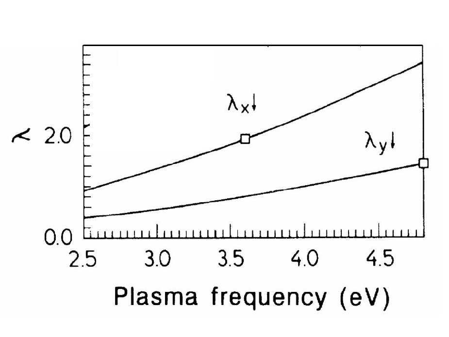
We shall argue in Subsection D that if one interprets the tunnelling experiments in systems near optimal doping [27]-[32] in the framework of the Eliashberg theory one obtains large EPI coupling constant which implies that . This means that EPI is reduced much more in transport properties than in the self-energy, which is due to some reasons that shall be discussed in Part II. Such a large reduction of cannot be obtained within the LDA-DFT band structure calculations which means that and contain renormalization which do not enter in the theory. In Part II we shall argue that the strong suppression of may have its origin in strong electronic correlations [51], [96] and in the long-range Madelung energy [2], [3].
4. Femtosecond time-resolved optical spectroscopy
The femtosecond time-resolved optical spectroscopy (FTROS) has been developed in the last couple of years and applied to HTSC cuprates. In this method a femtosecond ( ) laser pump excites in materials electron-hole pairs via interband transitions. These hot carriers release their energy via electron-electron (with the relaxation time ) and electron-phonon scattering reaching states near the Fermi energy within - see [98]. The typical energy density of the laser pump pulses with the wavelength nm ( ) was around (the excitation fluence ) which produces approximately carriers per pulse (by assuming that each photon produces carriers, is the superconducting gap). By measuring photoinduced changes of the reflectivity in time, i.e. , one can extract information on the relaxation dynamics of the low-laying electronic excitations. Since relax to equilibrium the fit with exponential functions is used
| (36) |
where ( is the Heavyside function) describes the finite rise-time. The parameters , depends on the fluence . This method was used in studying the superconucting phase of , with , and and respectively [26]. In that case one has for and for , while the signal was present also at . It turns out that the signal is related to the quasi-particle recombination across the superconducting gap and has a relaxation time of the order at . At the so called threshold fluence ( for and for ) the vaporization (destroying) of the superconducting phase occurs, where the parameter saturates. This vaporization process takes place at the time scala . The external fluence is distributed in the sample over the excitation volume which is proportional to the optical penetration depth ( at ) of the pump. The energy densities stored in the excitation volume at the vaporization threshold for and are and , respectively. The important fact is that is much larger than the superconducting condensation energy which is for and for , i.e. . This means that the energy difference must be stored elsewhere on the time scale . The only present reservoir which can absorb the difference in energy are the bosonic baths of phonons and spin fluctuations. The energy required to heat the spin reservoir from to is . The measured specific heat in [26] gives very small value . In the case of the phonon reservoir on obtains for and for , where is the phonon specific heat. Since the spin reservoir cannot absorb the rest energy . The situation is opposite with phonons since and phonon can absorb the rest energy in the excitation volume. The complete vaporization dynamics can be described in the framework of the Rothwarf-Taylor model which describes approaching of electrons and phonons to quasi-equilibrium on the time scale of 1 ps [99]. We shall not go into details but only summarize by quoting the conclusion in [99], that only phonon-mediated vaporization is consistent with the experiments, thus ruling out spin-mediated quasi-particle recombination and pairing in HTSC cuprates. The FTROS method tell us that at least for non-equilibrium processes EPI is more important than SFI. It gives also some opportunities for obtaining the strength of EPI but at present there is no reliable analysis.
In conclusion, optics and resistivity measurements in the normal state of cuprates give evidence that EPI is important while the spin fluctuation scattering is weaker than it is believed. However, some important questions related to the transport properties remain to be answered: (i) what are the values of and ; (ii) what is the reason that is realized in cuprates; (iii) what is the role of Coulomb scattering in and . Later on we shall argue that ARPES measurements in cuprates give evidence for an appreciable contribution of Coulomb scattering at higher frequencies, where for with . One should stress, that despite the fact that EPI is suppressed in transport properties it is sufficiently strong in the quasi-particle self-energy, as it comes out from tunnelling measurements discussed below.
III.3 ARPES and the EPI self-energy
The angle-resolved photoemission spectroscopy (ARPES) is nowadays one of leading spectroscopy methods in the solid state physics [12]. In some favorable conditions it provides direct information on the one-electron removal spectrum in a complex many body system. The method involves shining light (photons) with energies between on samples and by detecting momentum ()- and energy()-distribution of the outgoing electrons. The resolution of ARPES has been significantly increased in the last decade with the energy resolution of (for photon energies ) and angular resolution of . On the other side the ARPES method is surface sensitive technique, since the average escape depth () of the outgoing electrons is of the order of Å, depending on the energy of incoming photons. Therefore, very good surfaces are needed in order that the results to be representative for bulk samples. The most reliable studies were done on the bilayer () and its single layer counterpart (), since these materials contain weakly coupled planes with the longest inter-plane separation in the cuprates. This results in a natural cleavage plane making these materials superior to others in ARPES experiments. After a drastic improvement of sample quality in other families of HTSC materials, the ARPES technique has became an important method in theoretical considerations. The ARPES can indirectly give information on the momentum and energy dependence of the pairing potential. Furthermore, the electronic spectrum of the (above mentioned) cuprates is highly quasi-2D which allows rather unambiguous determination of the initial state momentum from the measured final state momentum, since the component parallel to the surface is conserved in photoemission. In this case, the ARPES probes (under some favorable conditions) directly the single particle spectral function . In the following we discuss mainly those ARPES experiments which give evidence for the importance of the EPI in cuprates - see more in [12].
ARPES measures a nonlinear response function of the electron system and it is usually analyzed in the so-called three-step model, where the total photoemission intensity is the product of three independent terms: (1) - describes optical excitation of the electron in the bulk; (2) - describes the scattering probability of the travelling electrons; (2) - the transmission probability through the surface potential barrier. The central quantity in the three-step model is and it turns out that for it can be written in the form [12] with and the quasi-particle spectral function Im
| (37) |
Here, is the dipole matrix element which depends on , polarization and energy of the incoming photons. The knowledge of the matrix element is of a great importance and its calculation from first principles was done in [100]. is the Fermi function, and are the quasi-particle Green’s function and the self-energy, respectively. We summarize and comment here some important ARPES results which were obtained in the last several years and which confirm the existence of the Fermi surface and importance of EPI in the quasi-particle scattering [12].
ARPES in the normal state
() There is well defined Fermi surface in the metallic state of optimally and near optimally doped cuprates with the topology predicted by the LDA-DFT. However, the bands are narrower than LDA-DFT predicts which points to a strong quasi-particle renormalization. () The spectral lines are broad with Im (or for ) which tells us that the quasi-particle liquid is a non-canonical Fermi liquid for larger values of . () There is a bilayer band splitting in (at least in the over-doped state) what is also predicted by LDA-DFT. In the case when the coherent hopping between two layers in the bilayer dominates, then the anti-bonding and bonding bands with have been observed. It is worth to mention that the previous experiments did not show this splitting what was one of the reasons for various speculations on some exotic electronic scattering and non-Fermi liquid scenarios. () In the under-doped cuprates and at temperatures there is a d-wave like pseudogap in the quasi-particle spectrum where increases by lowering doping. We stress that the pseudogap phenomenon is not well understood at present and since we are interested in systems near optimal doping where the pseudogap phenomena are absent or much less pronounced we shall not discuss this problem here. Its origin can be due to a precursor superconductivity or due to a competing order, such as spin- or charge-density wave, strong correlations, etc. () The ARPES self-energy gives evidence that EPI interaction is rather strong. The arguments for latter statement are the following: (i) at there are kinks in the quasi-particle dispersion in the nodal direction (along the line) at the characteristic phonon energy [60], see Fig. 14, and near the anti-nodal point at [101] - see Fig. 14.


(ii) This kink structure is observed in a variety of the hole-doped cuprates such as , , , (), (). These kinks exist also above what excludes the scenario with the magnetic resonance peak in . Moreover, since the tunnelling and magnetic neutron scattering measurements give small SFI coupling constant then the kinks can not be due to SFI. (iii) The position of the nodal kink is practically doping independent which points towards phonons as the scattering and pairing boson. () The quasi-particles (holes) at and near the nodal-point couple practically to a rather broad spectrum of phonons since at least three group of phonons were extracted in the bosonic spectral function from the ARPES effective self-energy in [102] - Fig. 15.

This result is in a qualitative agreement with numerous tunnelling measurements [27]-[32] which apparently demonstrate that the very broad spectrum of phonons couples with holes without preferring any particular phonons - see discussion below. () Recent ARPES measurements in B2212 [61] show very different slope of the quasi-particle energy at small and at large energies - see Fig. 16. The theoretical analysis [103] of these results gives the total coupling constant , and for the EPI coupling while the Coulomb coupling (SFI is a part of it) is [103] - see Fig. 16. (Note, that the upper index Z in the coupling constants means the quasi-particle renormalization in the normal part of the self-energy.) To this end let us mention some confusion which is related to the value of the EPI coupling constant extracted from ARPES. Namely, in [12], [104], [105] the EPI self-energy was obtained by subtracting the high energy slope of the quasi-particle spectrum at . The latter is apparently due to the Coulomb interaction. Although the position of the low-energy kink is not affected by this procedure (if ), this subtraction procedure gives in fact an effective EPI self-energy and the effective coupling constant only. We demonstrate below that the is smaller than the real EPI coupling constant . The total self-energy is where is the contribution due to the Coulomb interaction. At very low energies one has usually , where is the characteristic Coulomb energies and is the Coulomb coupling constant. The quasi-particle spectrum is determined from the condition where is the bare band structure energy. At low energies it can be rewritten in the form
| (38) |
with and
| (39) |
Since at very low energies , one has and , then the real coupling constant is related to the effective one by . At higher energies the EPI effects are suppressed and stops growing, one has . The measured at near and slightly away from the nodal point in the optimally doped Bi-2212 with [106] is shown in Fig. 16.

It is seen that has two kinks - the first one at low energy which is (as we already argued) most probably of the phononic origin [12], [104], [105], while the second kink at higher energy is due to the Coulomb interaction. However, the important results in Ref. [106] is that the slopes of at low () and high energies () are very different. The low-energy and high-energy slope near the nodal point are shown in Fig. 16 schematically (thin lines). From Fig. 16 it is obvious that EPI prevails at low energies . More precisely digitalization of in the interval gives the Coulomb coupling while the same procedure at gives the total coupling constant and the EPI coupling constant , i.e. the EPI coupling is at least twice larger than the effective EPI coupling constant obtained in the previous analysis of ARPES results [12], [104], [105]. This estimation tells us that at (and near) the nodal point, the EPI interaction dominates in the quasi-particle scattering at low energies since , while at large energies (compared to ), the Coulomb interaction with dominates. We point out that EPI near the anti-nodal point can be even larger than in the nodal point, mostly due to the higher density of states near the anti-nodal point. () Recent ARPES spectra in the optimally doped near the nodal and anti-nodal point [105] show a low energy isotope effect in , which can be well described in the framework of the Migdal-Eliashberg theory for EPI [107]. At higher energies the obtained in [105] very pronounced isotope effect cannot be explained by the simple Migdal-Eliashberg theory [107]. However, there are controversies with the strength of the high-energy isotope effect since it was not confirmed in other measurements [108], [109] - see the discussion in Section F.2 related to the isotope effects in HTSC cuprates. () ARPES experiments on give strong evidence for the formation of small polarons in undoped cuprates which are due to phonons and strong EPI, while by doping quasi-particles appear and there are no small polarons [110]. Namely, in [110] a broad peak around is observed at the top of the band () with the dispersion similar to that predicted by the model - see Fig. 17.

However, the peak in Fig. 17 (left) is of Gaussian shape and can be described only by coupling to bosons, i.e. this peak is a boson side band - see more in [6] and references therein. The theory based on the t-J model (in the antiferromagnetic state of the undoped compound) by including coupling to several (half-breathing, apical oxygen, low-lying) phonons, which is given in [111], explains successfully this broad peak of the boson side band by the formation of small polarons due to the EPI coupling (). Note that this value of is for the polaron at the bottom of the band while in the case where the Fermi surface exists (in doped systems) this coupling is even larger due to the larger density of states at the Fermi surface [111]. In [111] it was stressed that even when the electron-magnon interaction is stronger than EPI the polarons in the undoped systems are formed due to EPI. The latter mechanism involves excitation of many phonons at the lattice site (where the hole is seating), while it is possible to excite only one magnon at the given site. () Recent soft x-ray ARPES measurements on the electron doped HTSC [112], and ( ), , [113] show kink at energies in the quasi-particle dispersion relation along both nodal and antinodal directions as it is shown in Fig. 18.

It is seen from this figure that the effective EPI coupling constant is isotropic and . It seems that the kink in the electron-doped cuprates is due solely to EPI and in that respect the situation is similar to the one in the hole-doped cuprates.
ARPES results in the superconducting state
() There is an anisotropic superconducting gap in most HTSC compounds [12], which is predominately d-wave like, i.e. with . () The particle-hole coherence in the superconducting state which is expected for the BCS-like theory of superconductivity has been observed first in [114] and confirmed with better resolution in [115], where the particle-hole mixing is clearly seen in the electron and hole quasi-particle dispersion. To remaind the reader, the excited Bogoliubov-Valatin quasi-particles () with energies are a mixture of electron () and hole (), i.e. , where the coherence factors , are given by . Note, that what is exactly observed, together with d-wave pairing , in experiments [115]. This is very important result since it proves that the pairing in HTSC cuprates is of the BCS type and not exotic one as was speculated long time after the discovery of HTSC cuprates. () The kink at in the quasi-particle energy around the nodal point is not shifted (in energy) while the antinodal kink at is shifted (in energy) in the superconducting state by , i.e. [12]. To remind the reader, in the standard Eliashberg theory the kink in the normal state at should be shifted in the superconducting state to at all points at the Fermi surface. This puzzling result (that the quasi-particle energy around the nodal point is not shifted in the superconducting state) might be a smoking gun result since it makes an additional constraint on the quasi-particle interaction in cuprates. Until now there is only one plausible explanation [116] of this non-shift puzzle which is based on an assumption of the forward scattering peak (FSP) in EPI - see more in Part II. The FSP in EPI means that electrons scatter into a narrow region () around the initial point in the -space, so that at the most part of the Fermi surface there is practically no mixing of states with different signs of the order parameter . In that case the EPI bosonic spectral function (which is defined in Appendix A) ( is the angle on the Fermi surface) has a pronounced forward scattering peak (at ) due to strong correlations - see Part II. Its width is narrow, i.e and the angle integration goes over the region around the point . In that case the kink is shifted (approximately) by the local gap - for more details see [116]. As the consequence, the anti-nodal kink is shifted by the maximal gap, i.e. while the nodal gap is practically unshifted since . () The recent ARPES spectra [117] on an undoped single crystalline 4-layered cuprate with apical fluorine (F), (F0234) give rather convincing evidence against the SFI mechanism of pairing - see Fig. 19.

First, F0234 is not a Mott insulator - as expected from valence charge counting which puts valence as , but it is a superconductor with . Moreover, the ARPES data [117] reveal at least two metallic Fermi-surface sheets with corresponding volumes equally below and above half-filling - see Fig. 20.

Second, one of the Fermi-surfaces is due to the electron-like () band (with % electron-doping) and the other one due to the hole-like () band (with hole-doping) and their splitting along the nodal direction is significant and cannot be explained by the LDA-DFT calculations [118]. This electron and hole self-doping of inner and outer layers is in an appreciable contrast to other multilayered cuprates where there is only hole self-doping. For instance, in HgBa2CanCun+1O2n+2 () and (Cu,C)Ba2CanCun+1O3n+2 (), the inner CuO2 layers are less hole-doped than outer layers. It turns out, unexpectedly, that the superconducting gap on the -band Fermi-surface is significantly larger than on the -one, where in the ratio is anomalous and is an order of magnitude larger than in the electron-doped cuprate . Third, the -band Fermi-surface is rather far from the antinodal point at (). This is very important result which means that the antiferromagnetic spin fluctuations with the AF wave-vector , as well as the van Hove singularity, are not dominant in the pairing in the -band. To remind the reader, the SFI scenario assumes that the pairing is due to spin fluctuations with the wave-vector (and near it) which connects two anti-nodal points which are near the van Hove singularity at the hole-surface (at () and ()) giving rise to large density of states. This is apparently not the case for the -band Fermi-surface - see Fig. 20. The ARPES data give further that there is a kink at in the quasi-particle dispersion of both bands, while the kink in the -band is stronger than that in the -band. This result, together with the anomalous ratio , strongly disfavors SFI as a pairing mechanism. () Despite the presence of significant elastic quasi-particle scattering in a number of samples of optimally doped Bi-2212, there are dramatic sharpening of the spectral function near the anti-nodal point at (in the superconducting state) [119]. This effect can be explained by assuming that the small -scattering (the forward scattering peak) dominates in the elastic impurity scattering as it is pointed in [51], [96], [120], [121]. As a result, one finds that the impurity scattering rate in the superconducting state is almost zero, i.e. for for any kind of pairing (- - -wave etc.) since the normal () and the anomalous () scattering rates compensate each other. This collapse of the elastic scattering rate is elaborated in details in [119] and it is a consequence of the Anderson-like theorem for unconventional superconductors which is due to the dominance of the small -scattering [51], [96], [120]-[121]. In such a case -wave pairing is weakly unaffected by impurities and there is small reduction in [121], [122]. The physics behind this result is rather simple. The small -scattering (usually called forward scattering) means that electrons scatter into a small region in the k-space, so that at the most part of the Fermi surface there is no mixing of states with different signs of the order parameter . In such a way the detrimental effect of impurities on -wave pairing is significantly reduced. This result points to the importance of strong correlations in the renormalization of the impurity scattering too - see discussion in Part II.
In conclusion, in order to explain ARPES results in cuprates it is necessary to take into account: (1) the electron-phonon interaction (EPI) since it dominates in the quasi-particle scattering in the energy region important for pairing; (2) effects of elastic nonmagnetic impurities with the forward scattering peak (FSP) due to strong correlations; (3) the Coulomb interaction which dominates at higher energies . In this respect, the presence of ARPES kinks and the knee-like shape of the T-dependence of the spectral width are important constraints on the scattering and pairing mechanism in HTSC cuprates.
III.4 Tunnelling spectroscopy and spectral function
By measuring current-voltage characteristics in (normal metal-insulator-superconductor) tunnelling junctions with large tunnelling barrier one obtains from tunnelling conductance the so called tunnelling density of states in superconductors . Moreover, by measuring of at voltages it is possible to determine the Eliashberg spectral function and finally to confirm the phonon mechanism of pairing in materials. Four tunnelling techniques were used in the study of cuprates: vacuum tunnelling by using the technique - scanning tunnelling microscope; point-contact tunnelling; break-junction tunnelling; planar-junction tunnelling. Each of these techniques has some advantages although in principle the most potential one is the STM technique since it measures superconducting properties locally [123]. Since tunnelling measurements probe a surface region of the order of superconducting coherence length , then this kind of measurements in materials with small coherence length ( Å in the plane and Å along the ) depends strongly on the surface quality and sample preparation. Nowadays, many of the material problems in cuprates are understood and as a result consistent picture of tunnelling features is starting to emerge.
From tunnelling experiments one obtains the (energy dependent) gap function in the superconducting state. Since we have already discussed this problem in [3], we will only briefly mention some important result, that in most cases has -shape in all families of HTSC hole and electron doped cuprates. The -shape is characteristic for pairing with gapless spectrum, which is also confirmed in the interference experiments on hole and electron doped cuprates [48]. Some experiments give an -shape of which resembles -wave pairing. This controversy is explained to be the property of the tunnelling matrix element which filters out states with the maximal gap.
Here we are interested in the bosonic spectral function of HTSC cuprates near optimal doping which can be extracted by using tunnelling spectroscopy. We inform the reader in advance, that the shape and the energy width of , which are extracted from the second derivative at voltages above the superconducting gap, in most HTSC cuprates resembles the phonon density of states . This result is strong evidence for the importance of in the pairing potential of cuprates. For instance, plenty of break-junctions made from single crystals [27] show that the peaks (and shoulders) in (or dips-negative peaks in ) coincide with the peaks (and shoulders) in the phonon density of states measured by neutron scattering - see Fig. 21.

The tunnelling spectra in Bi-2212 break junctions [27], which are shown in Fig. 21, indicates that the spectral function is independent of magnetic field, which is in contradiction with the theoretical prediction based on the SFI pairing mechanism where this function should be sensitive to magnetic field. The reported broadening of the peaks in are partly due to the gapless spectrum of pairing in cuprates. Additionally, the tunnelling density of states at very low and for show a pronounced gap structure. It was found that , where and is some average value of the gap. In order to obtain the inverse procedure was used by assuming superconductivity and the effective Coulomb parameter [27]. The obtained gives large coupling constant . Although this analysis [27] was done in terms of pairing, it mimics qualitatively the case of pairing, since one expects that pairing does not change significantly the global structure of at albeit introducing a broadening in it - see the physical meaning in Appendix A. We point out that the results obtained in [27] were reproducible on more than junctions. In that respect very important results on slightly overdoped and on planar tunnelling junctions are obtained in [28] - see Fig. 22.

These results show very similar features to those obtained in [27] on break-junctions. It is worth mentioning that several groups [29], [30], [31] have obtained similar results for the shape of the spectral function from the measurements on various cuprates - see the comparison in Fig. 23. These facts leave no much doubts about the importance of the in pairing mechanism of cuprates.

In that respect, tunnelling measurements on slightly overdoped [28], [32] give impressive results. The Eliashberg spectral function of this compound was extracted from the measurements of and by solving the inverse problem - see Appendix A. The extracted has several peaks in broad energy region up to as it is seen in Figs. 22-23, which coincide rather well with the peaks in the phonon density of states - more precisely the generalized phonon density of states defined in Appendix A. In [32] numerous peaks, from , in are discerned as shown in Fig. 24, which correspond to various groups of phonon modes - laying in (and around) these peaks. Moreover, in [28], [32] the coupling constants for these modes are extracted as well as their contribution () to as it is seen in Fig. 25. Note, that due to the nonlinearity of the problem the sum of is not equal to .

The next remarkable result is that the extracted coupling constant is
very large, i.e. - see Fig. 25. It is obvious
from Figs. (24-25) that almost all
phonon modes contribute to and , which means that on
the average each particular phonon mode is not too strongly coupled to
electrons since , thus keeping the lattice stable.

For a better understanding of the the EPI coupling in these systems we show in Fig. 26 the total and partial density of phononic states. Let us discuss the content of the Table in Fig. 25 in more details where it is shown the strength of the EPI coupling and the relative contribution of different phononic modes to .

In Fig. 25 it is seen that lower frequency modes from , corresponding to and vibrations, are rather strongly coupled to electrons (with ) which give appreciable contributions to . It is also seen in Fig. 25 that the coupling constants of the high-energy phonons ( with ) have and give moderate contribution to - around . These results give solid evidence for the importance of the low-energy modes related to the change of the Madelung energy in the ionic-metallic structure of HTSC cuprates - the idea advocated in [2], [3] and discussed in Part II. If confirmed in other HTSC families, these results are in favor of the moderate oxygen isotope effect in cuprates near the optimal doping since the oxygen modes are higher energy modes and gives smaller contribution to . We stress that each peak in corresponds to many modes. In order to obtain information on the structure of vibrations which are strongly involved in pairing, we show in Figs. 27-28 the structure of these vibrations at special points in the Brillouin zone. It is seen in Fig. 27 that the low-frequency phonons are dominated by , , vibrations.


Further, based on the Table in Fig. 25 one can conclude that the modes are stronger coupled to electrons than ones, although the density of state for the modes is larger. The reason for such an anomalous behavior might be due to symmetries of the corresponding phonons as it is seen in Fig. 28. Namely, to the peak contribute axial vibrations of in the plane which are odd under inversion, while in the peak these modes are even. The in-plane modes of and are present in which are in-phase and out-of-phase modes, while in they are all out-of-phase modes. For more information on other modes see [32]. We stress that the Eliashberg equations based on the extracted of the slightly overdoped with the ratio describe rather well numerous optical, transport and thermodynamic properties [32]. However, in underdoped systems with , where the pseudogap phenomena are pronounced, there are serious disagreements between experiments and the Migdal-Eliashberg theory [32]. We would like to stress that the contribution of the high frequency modes (mostly the oxygen modes) to may be underestimated in tunnelling measurements due to their sensitivity to surface contamination and defects. Namely, the tunnelling current probes a superconductor to a depth of order of the quasi-particle mean-free path . Since decreases with increasing the mean free path can be rather small and the effects of the high energy phonons are sensitive to the surface contamination.
Similar conclusion regarding the structure of the spectral function in cuprates comes out from tunnelling measurements on Andreev junctions ( - low barrier) and Giaver junctions ( - high barrier) in and compounds [125], where the extracted is in good accordance with the phonon density of states - see Fig. 29.

Note, that the BTK parameter is related to the transmission and reflection coefficients for the normal metal and respectively.
Although most of the peaks in of cuprates coincide with the peaks in the phonon density of states it is legitimate to put the question - can the magnetic resonance in the superconducting state give significant contribution to ? In that respect the inelastic magnetic neutron scattering measurements of the magnetic resonance as a function of doping [126] give that the resonance energy scales with , i.e. as shown in Fig.30.

This means that if one of the peaks in is due to the magnetic resonance at , then it should shift strongly with doping as it is observed in [126]. This is contrary to phonon peaks (energies) whose positions are practically doping independent. To this end, recent tunnelling experiments on Bi-2212 [33] show clear doping independence of as it is seen in Fig. 31. This remarkable result is an additional and strong evidence in favor of EPI and against the SFI mechanism of pairing in HTSC cuprates which is based on the magnetic resonance peak in the superconducting state. In that respect the analysis in [127] of tunneling spectra of electron-doped cuprates Pr with shows the existence of the bosonic mode at which is significantly larger than the magnetic-resonance mode with . This result excludes the magnetic-resonance mode as an important factor which modifies superconductivity.

The presence of pronounced phononic structures (and the importance of EPI) in the characteristics was quite recently demonstrated by the tunnelling measurements on the very good films prepared by the molecular beam epitaxy on the [001]-symmetric bi-crystal substrates [34]. They give unique evidence for eleven peaks in the (negative) second derivative, i.e. . Furthermore, these peaks coincides with the peaks in the intensities of the phonon Raman scattering data measured at in single crystals of LSCO with of Sr [35]. These results are shown in Fig. 32. In spite of the lack of a quantitative analysis of the data in the framework of the Eliashberg equations the results in Ref. [34] are important evidence that phonons are relevant pairing bosons in HTSC cuprates.

It is interesting that in the -axis vacuum tunnelling measurements [128] the fine structure in at was not seen below , while the pseudogap structure is observed at temperatures near and above . This result could mean that the tunnelling is likely dominated by the nontrivial structure of the tunnelling matrix element (along the -axis), which is derived from the band structure calculations [129]. However, recent experiments on [39] give information on possible nature of the bosonic mode which couples with electrons. In [39] the local conductance is measured where it is found that has peak at where has the maximal slope - see Fig. 33(a).


It turns out that the corresponding average phonon energy depends on the oxygen mass, i.e. , with and - as it is seen in Fig. 33(b). This result is interpreted in [39] as an evidence that oxygen phonons are strongly involved in the quasi-particle scattering. A possible explanation is put forward in [39] by assuming that this isotope effect is due to the B1g phonon which interacts with the anti-nodal quasi-particles. However, this result requires a reanalysis since the energy of the bosonic mode in fact coincides with the dip and not with the peak of - as reported in [39].
The important message of most tunnelling experiments in cuprates near and at the optimal doping is that there is strong evidence for the importance of in the quasi-particle scattering and that no particular phonon mode can be singled out in the spectral function as being the only one which dominates in pairing mechanism. This important result means that the high is not attributable to a particular phonon mode in the mechanism but all phonon modes contribute to . Having in mind that the phonon spectrum in cuprates is very broad (up to ), then the large constant () obtained in tunnelling experiments is not surprising at all. Note, that similar conclusion holds for some other oxide superconductors such as with where the peaks in the bosonic spectral function /extracted from tunnelling measurements) coincide with the peaks in the phononic density of states [130], [131]).
III.5 Phonon spectra and EPI
Although experiments related to phonon spectra and their renormalization by , such as inelastic neutron, inelastic x-ray and Raman scattering, do not give the spectral function they nevertheless can give useful, but indirect, information on the strength of EPI for some particular phonons. We stress in advance that the interpretation of experimental results in HTSC cuprates by the theory of EPI for weakly correlated electrons is risky since in strongly correlated systems, such as HTSC cuprates, the phonon renormalization due to EPI is different than in weakly correlated metals [132]. Since these questions are reviewed in [132] we shall briefly enumerate the main points: (1) in strongly correlated systems the EPI coupling for a number of phononic modes can be significantly larger than the LDA-DFT and Hartree-Fock methods predict. This is due to many-body effects not contained in LDA-DFT [132], [133]. The lack of the LDA-DFT calculations in obtaining phonon line-widths is clearly demonstrated, for instance in experiments on L2-xSrxCuO4 - see review [134] and References therein, where the bond-stretching phonons at are softer and much broader than the LDA-DFT calculations predict. (Note, the wave vector is in units () - for instance in these units corresponds to .) (2) The calculation of phonon spectra is in principle very difficult problem since besides the complexity of structural properties in a given material one should take into account appropriately the long-range Coulomb interaction of electrons as well as strong short-range repulsion. Our intention is not to discuss this complexity here - for that see for instance in [44], but we only stress some important points which will help to understand problems with which is confronted the theory of phonons in cuprates.
The phonon Green’s function depends on the phonon self-energy which takes into account all the enumerated properties (note ). In cases when the EPI coupling constant is a function on the transfer momentum only, then () depends on the quasi-particle charge susceptibility
| (40) |
and is the irreducible electronic polarization given by
| (41) |
The screening due to the long-range Coulomb interaction is contained in the electronic dielectric function while the”screening” due to (strong) correlations is described by the charge vertex function . Due to complexity of the physics of strong correlations the phonon dynamics was studied in the model but without the long-range Coulomb interaction [132], [133], [135], in which case one has and . However, in studying the phonon spectra in cuprates it is expected that this deficiency is partly compensated by choosing the bare phonon frequency (contained in ) to correspond to undoped compounds [132], [135]. It is a matter of future investigations to incorporate all relevant interactions in order to obtain a fully microscopic and reliable theory of phonons in cuprates. Additionally, the electron-phonon interaction (with the bare coupling constant ) is dominated by the change of the energy of the Zhang-Rice singlet - see more Part II Section VII, and in that Eq.(40) for is adequate one [3], [132], [133]. Since the charge fluctuations in HTSC cuprates are strongly suppressed (no doubly occupancy of the Cu 3d9 state) due to strong correlations and since the suppressed value of can not be obtained by the band-structure calculations this means that LDA-DFT underestimates the EPI coupling constant significantly. In the following we discuss this important result briefly.
III.5.1 Inelastic neutron and x-ray scattering - phonon softening and width due to EPI
The softening and broadening of numerous phonon modes has been observed in the normal state of cuprates giving evidence for pronounced EPI effects and for inadequacy of the LDA-DFT calculations in treating strong correlations and suppression of the charge susceptibility [3], [6], [132], [135]. There are several relevant reviews on this subject [6] , [134], [132], [136] and here we discuss briefly two important examples which demonstrate the inefficiency of the LDA-DFT band structure calculations to treat quantitatively EPI in HTSC cuprates. For instance, the Cu-O bond-stretching phonon mode shows a substantial softening at by doping of and [134], [136] - called the half-breathing phonon, and a large broadening by at doping [140] as it is seen in Fig. 34. While the softening can be partly described by the LDA-DFT method [137], the latter theory predicts an order of magnitude smaller broadening than the experimental one. This failure of LDA-DFT is due to incorrect treatment of the ffects of strong correlations on the charge susceptibility and due to absence of many body effects which can increase the coupling constant - see more in Part II. The neutron scattering measurements in give evidence for large ( ) softening of the with symmetry with the energy , which is theoretically predicted in [138], and for the large line-width about which also suggests strong EPI. These apex modes are favorable for -wave pairing since their coupling constants are peaked at small momentum [6]. Having in mind the above results, there is not surprising at all that the recent calculations of the EPI coupling constant in the framework of LDA-DFT give very small EPI coupling constant [16], [17]. The critical analysis of the LDA-DFT results in HTSC cuprates is done in [3] and recently additionally argued in [6], [139] by their disagreement with inelastic neutron and x-ray scattering measurements - as it is shown in Fig. 34.

In Part II we shall discuss some theoretical approaches related to EPI in strongly correlated systems but we shall not study the phonon renormalization. The latter problem was studied more detailed and thoroughly in the review article [6], [134]. Here, we point out only three important results. First, there is an appreciable difference in the phonon renormalization in strongly and weakly correlated systems. Namely, the change of phonon frequencies in the presence of conduction electrons is proportional to the squared coupling constant and charge susceptibility , i.e. , while the line width is given by . All these quantities can be calculated in LDA-DFT and as we discussed above where for some modes one obtains that . However, it turns out that in strongly correlated systems doped by holes (with the concentration ) the charge fluctuations are suppressed in which case the following sum-rule holds [6], [135]
| (42) |
while in the LDA-DFT method one has
| (43) |
The inequality (for some phonon modes) together with Eqs.(42-43) means that for low doping the LDA strongly underestimates the EPI coupling constant in the large portion of the Brillouin zone, i.e. one has . The large softening and the large line width of the half-breathing mode at but very moderate effects for the breathing mode at is explained in the framework of the one slave-boson (SB) theory (for ) in [135], where (i.e. ) is calculated in leading order. We stress that there is another method for studying strong correlations - the X-method, where the controllable expansion is performed in terms of Hubbard operators and where the charge vertex is calculated [3], [51], [96], [97]. It turns out that in the adiabatic limit () the vertex functions in two methods have some important differences. For instance, (in the X-method) is peaked at - the so called forward scattering peak, while has maximum at finite [141] - see Part II, Section VI.E. The properties of are confirmed by numerical Monte Carlo calculations in the finite-U Hubbard model [168], where it is found that FSP exists for all , but it is especially pronounced in the limit . These results are also confirmed in [171] where the calculations are performed in the four slave-bosons technique - see more Part II Section VII.E. Having in mind this difference it would be useful to have calculations of in the framework of the X-method which are unfortunately not done yet. Second, the many body theory gives that for coupling to some modes the coupling constant in HTSC cuprates can be significantly larger than LDA-DFT predicts [6], which is due to some many-body effects not present in the latter [133]. In Part II it will be argued that for some phonon modes one has . For instance, for the half-breathing mode, one has [6], [133] - see Part II. These two results point to an inadequacy of LDA-DFT in calculations of EPI effects in HTSC cuprates. Third, the phonon self-energy () and quasi-particle self-energy are differently renormalized by strong correlations [3], [6], [51], [96], [97], which is the reason that is much more suppressed than - see Part II. The effects of the charge vertex on and are differently manifested. Namely, the vertex function enters quadratically in and the presence of the forward scattering peak in the charge vertex strongly affects the EPI coupling constant in
| (44) |
where is the quasi-particle Green’s function, is the quasi-particle vertex and is the Hubbard quasi-particle spectral weight - see Part II, Section VII. In the adiabatic limit one has and for the charge vertex is strongly suppressed () making the effective EPI coupling (which also enters the pairing potential) small at large (transfer) momenta . This has strong repercussion on the pairing due to EPI since for small doping it makes the d-wave pairing coupling constant to be of the order of the s-one (). Then in the presence of the residual Coulomb interaction EPI gives rise to d-wave pairing. On the other side the charge vertex enters linearly and it is additionally integrated over the quasi-particle momentum - see Eq.(41). Therefore, one expects that the effects of the forward scattering peak on are less pronounced than on . Nevertheless, the peak of at may be (partly) responsible that the maximal experimental softening and broadening of the stretching (half-breading) mode in and is at [134] and not at for which reaches maximum. This means that the charge vertex function pushes the renormalized EPI coupling constant to smaller . It would be very interesting to have calculations for other phonons by including the vertex function obtained by the X-method - see Section.VII
III.5.2 The phonon Raman scattering
The phonon Raman scattering gives an indirect evidence for importance of EPI in cuprates [142], [143], [144]. We enumerate some of them - see more in [3] and References therein. (i) There is a pronounced asymmetric line-shape (of the Fano resonance) in the metallic state. For instance, in two Raman modes at ( dominated mode) and at ( dominated mode in the planes) show pronounced asymmetry which is absent in . This asymmetry means that there is an appreciable interaction of Raman active phonons with continuum states (quasi-particles). (ii) The phonon frequencies for some and are strongly renormalized in the superconducting state, between , pointing again to the importance of EPI [144] - see also in [3], [23]. To this point we mention that there is a remarkable correlation between the electronic Raman cross-section and the optical conductivity in the plane , i.e. [3]. In previous Subsections it is argued that EPI with the very broad spectral function ( ) explains in a natural way the and dependence of . This means that the electronic Raman spectra in cuprates can be explained by EPI in conjunction with strong correlations. This conclusion is supported by calculations of the Raman cross-section [145] which take into account EPI with extracted from tunnelling measurements in and [3], [27]-[32]. Quite similar properties (to cuprates) of the electronic Raman scattering, as well as of , and , were observed in experiments [74] on isotropic 3D metallic oxides and where there are no signs of antiferromagnetic fluctuations. This means that low-dimensionality and antiferromagnetic spin fluctuations cannot be a prerequisite for anomalous scattering of quasi-particles and EPI must be inevitably taken into account since it is present in all these compounds.
III.6 Isotope effect in and
The isotope effect in the critical temperature was one of the very important proof for the EPI pairing in low-temperature superconductors (LTSC). As a curiosity the isotope effect in systems was measured almost exclusively in mono-atomic systems and in few polyatomic systems: the hydrogen isotope effect in , the and isotope shift of in , and the isotope effect in and . We point out that very small ( in and ) and even negative (in ) isotope effect in some polyatomic systems of materials are compatible with the pairing mechanism but in the presence of substantial Coulomb interaction or lattice anharmonicity. The isotope effect cannot be considered as the smoking gun effect since it is sensitive to numerous influences. For instance, in it is with certainty proved that the pairing is due to EPI and strongly dominated by the boron vibrations, but the boron isotope effect is significantly reduced, i.e. and the origin for this smaller value is still unexplained. The situation in HTSC cuprates is much more complicated because they are strongly correlated systems and contain many-atoms in unit cell. Additionally, the situation is complicated with the presence of intrinsic and extrinsic inhomogeneities, low dimensionality which can mask the isotope effects. On the other hand new techniques such as ARPES, STM, allow studies of the isotope effects in quasi-particle self-energies, i.e. , which will be discussed below.
III.6.1 Isotope effect in
This problem will be discussed only briefly since more extensive discussion can be found in [3]. It is well known that in the pure EPI pairing mechanism, the total isotope coefficient is given by , where is the mass of the i-th element in the -th crystallographic position. We stress that the total isotope effect is not measured in HTSC cuprates but only some partial ones. Note, that in the case when the screened Coulomb interaction is negligible, i.e. , the theory predicts . From this formula one can deduce that the relative change of , , for heavier elements should be rather small - for instance it is for , for and for . This means that measurements of for heavier elements are at/or beyond the ability of present day experimental techniques. Therefore most isotope effect measurements were done by substituting light atoms by only. It turns out that in most optimally doped HTSC cuprates is rather small. For instance in with , but it is appreciable in with where. In with one has while and even negative () in with . The experiments on () with are still unreliable and is unknown. In the electron-doped with one has while in the underdoped materials increases. The largest is obtained even in the optimally doped compounds like in systems with substitution, such as , , where for . In there is a isotope effect which is of the order of the oxygen one, i.e. giving for optimally doped systems (). In case when with one has with [146]. The appreciation of copper isotope effect in tells us that vibrations other than oxygen ions are important in giving high Tc. In that sense one should have in mind the tunnelling experiments discussed above, which tell us that all phonons contribute to the Eliashberg pairing function and according to these results the oxygen modes give moderate contribution to [32]. Hence the small oxygen isotope effect in optimally doped cuprates, if it is an intrinsic property at all (due to pronounced local inhomogeneities of samples and quasi-two dimensionality of the system), does not exclude the EPI mechanism of pairing.
III.6.2 Isotope effect in the self-energy
The fine structure of the quasi-particle self-energy , such as kinks and slopes, can be resolved in ARPES measurements and in some respect in STM. It turns out that there is isotope effect in the self-energy in the optimally doped samples [105], [108], [109]. In the first paper on this subject [105] it is reported a red shift of the nodal kink at for the substitution. In [105] it is reported that the isotope shift of the self-energy is very pronounced at large energies . Concerning the latter result, there is a dispute since it is not confirmed experimentally in [108], [109]. However, the isotope effect in at low energies [108], [109] is well described in the framework of the Migdal-Eliashberg theory for EPI [107] which is in accordance with the recent ARPES measurements with low-energy photons [147]. The latter allowed very good precision in measuring the isotope effect in the nodal point of Bi-2212 with and [147]. They observed shift in the maximum of - at (it corresponds to the half-breathing or to the breathing phonon) by as shown in Fig. 35.

By analyzing the shift in Im - shown in Fig. 35, one finds similar result for . The similar shift was obtained in STM measurements [39] which is shown in Fig. 33(b) and can have its origin in different phonons. We would like to stress two points: () in compounds with the oxygen isotope effect in is moderate, i.e. , [147]. If we consider this value to be intrinsic then even in this case it is not in conflict with the tunnelling experiments [32] since the latter give evidence that vibrations of heavier ions contribute significantly to - see the discussion in Subsection D on the tunnelling spectroscopy; () in ARPES measurements of [147] the effective EPI coupling constant is extracted, while the theory in Subsection C gives that the real coupling constant is larger, i.e. . This value is significantly larger than the LDA-DFT theory predicts [16], [17]. This again points that the LDA-DFT method does not pick up the many-body effects due to strong correlations- see Part II.
IV Summary of Part I
The analysis of experimental data in HTSC cuprates which are related to optics, tunnelling and ARPES measurements near and at the optimal doping give evidence for the large electron-phonon interaction (EPI) with the coupling constant . We stress that this analysis is done in the framework of the Migdal-Eliashberg theory for EPI which is a reliable approach for systems near the optimal doping. The spectral function , averaged over the Fermi surface, is extracted from various tunnelling measurements on bulk materials and tin films. It contains peaks at the same energies as the phonon density of states . So obtained spectral function when inserted in the Eliashberg equations provides sufficient strength for obtaining high critical temperature T . These facts are a solid proof for the important role of EPI in the normal state scattering and pairing mechanism of cuprates. Such a large (experimental) value of the EPI coupling constant and the robustness of the d-wave superconductivity in the presence of impurities imply that the EPI and impurity scattering amplitude must be strongly momentum dependent. The IR optical reflectivity data provide additional support for the importance of EPI since by using the spectral function (extracted from tunnelling measurements) one can quantitatively explain frequency dependence of the dynamical conductivity, optical relaxation rate and optical mass. These findings related to EPI are additionally supported by ARPES measurements on BISCO compounds. The ARPES kinks, the phononic features and isotope effect in the quasi-particle self-energy in the nodal and anti-nodal points at low energies () persist in the normal and superconducting state. They are much more in favor of EPI than for the spin fluctuation (SFI) scattering mechanism. The transport EPI coupling constant in HTSC cuprates is much smaller than , i.e. , which points to some peculiar scattering mechanism not met in low-temperature superconductors. The different renormalization of the quasi-particle and transport self-energies by the Coulomb interaction (strong correlations) hints to the importance of the small-momentum scattering in EPI. This will be discussed in Part II.
The ineffectiveness of SFI to solely provide pairing mechanism in cuprates comes out also from magnetic neutron scattering on YBCO, BISCO. As a result, the imaginary part of the susceptibility is drastically reduced in the low energy region by going from slightly underdoped toward optimally doped systems, while is practically unchanged. This implies that the real SFI coupling constant is small since the experimental value is much smaller than the assumed theoretical value .
Inelastic neutron and x-ray scattering measurements in cuprates show that the broadening of some phonon lines is by an order of magnitude larger than the LDA-DFA methods predict. Since the phonon line-widths depend on the EPI coupling and the charge susceptibility it is evident that calculations of both quantities are beyond the range of applicability of LDA-DFT. As a consequence, LDA-DFT overestimates electronic screening and thus underestimates the EPI coupling, since many-body effects due to strong correlations are not contained in this mean-field type theory. However, in spite of the promising and encouraging experimental results about the dominance of EPI in cuprates the theory is still confronted with difficulties in explaining sufficiently large coupling constant in the d-channel. At present there is no such a satisfactory microscopic theory although some concepts, such as the the dominant EPI scattering at small transfer momenta, are understood at least qualitatively. These set of problems and questions will be discussed in Part II.
Part II Theory of EPI in HTSC
The experimental results in Part I give evidence that the electron-phonon interaction (EPI) in HTSC cuprates is strong and in order to be conform with -wave pairing EPI must be peaked at small transfer momenta. A number of other experiments in HTSC cuprates give evidence that these are strongly correlated systems with large on-site Coulomb repulsion of electrons on the Cu-ions. However, at present there is no satisfactory microscopic theory of pairing in HTSC cuprates which is capable to calculate and the order parameter. This is due to mathematical difficulties in obtaining a solution of the formally exact ab initio many-body equations which take into account two important ingredients - EPI and strong correlations [3]. In Section V we discuss first the ab initio many body theory of superconductivity in order to point places which are most difficult to be solved. Since the superconductivity is low energy phenomenon (also in HTSC cuprates) one can simplify the structure of the ab initio equations in the low-energy sector (the Migdal-Eliashberg theory) where the high-energy processes are incorporated in the (so called) ideal band structure (non-local) potential and vertex functions . Due to its complexity this program of calculation of , , EPI couplings is not realized in HTSC superconductors. However, one pragmatical way out is to calculate in the framework of the LDA-DFT method which is at present stage unable to treat strong correlations in a satisfactory manner. Some achievements and results of LDA-DFT which are related to HTSC cuprates are discussed in Section VI.
In the case of very complicated systems, such as the HTSC cuprates, the standard (pragmatical) procedure in physics is to formulate a minimal theoretical model - sometimes called toy model, which includes minimal set of important ingredients necessary for qualitative and and semi-quantitative study of a phenomenon. As the consequence of the experimental results, the minimal theoretical model for cuprates must comprise two important ingredients: 1. EPI and 2. strong correlations. In Section VII we shall introduce such a minimal theoretical model which includes EPI and discuss the renormalization of EPI by strong correlations. In recent years the interest in this set of problems is increased and numerous numerical calculations were done mostly on small clusters with atoms (). We shall not discuss this subject which is fortunately covered in the recent comprehensive review [6]. The analytical approaches in studying the renormalization of EPI by strong correlations, which are based on a controllable and systematic theory, are rather scarce. We shall discuss such a systematic and controllable theory in the framework of the model with , which is formulated and solved in terms of Hubbard operators. The theory of this (toy) model predicts some interesting effects which might be important for understanding the physics of HTSC cuprates. It predicts that the high-energy processes (due to the suppression of doubly occupancy for ) give rise to a nonlocal contribution to the band structure potential (self-energy ) as well as to EPI. This non-locality in EPI is responsible for the peak in the effective pairing potential () at small transfer momenta () [3], [51], [96]. The latter property allows that the (strong) EPI is conform with d-wave pairing in HTSC cuprates. Furthermore, the peculiar structural properties of HTSC cuprates and corresponding electronic quasi-two-dimensionality give an additional non-locality in EPI. The latter is due to the weakly screened Madelung energy for a number of lattice vibrations along the c-axis. Since at present there is no quantitative theory for the latter effect we tackle this problem here only briefly. The next task for the future studies of the physics of HTSC cuprates is to incorporate these structural properties in the minimal theoretical model problem.
Finally, by writing this chapter our intention is not to overview the theoretical studies of EPI in HTSC cuprates - an impossible task, but more (i) to elucidate the descending way from the (old) well-defined ab initio microscopic theory of superconductivity to the one of the minimal model which treats the interplay of EPI and strong correlations, (ii) to encourage the reader to further develop the theory of HTSC cuprates.
V Microscopic theory of superconductivity
V.1 Ab iniitio many-body theory
The many-body theory of superconductivity is based on the fully microscopic electron-ion Hamiltonian for electrons and ions in the crystal - see for instance [148], [149]. It comprises mutually interacting electrons which also interact with ions and ionic vibrations. In order to pass continually to the problem of interplay of EPI and strong correlations and also to explain why the LDA-DFT method is inadequate for HTSC cuprates we discuss this problem here with restricted details - more extended discussion can be found in [3], [149]. In order to describe superconductivity the Nambu-spinor is introduced which operates in the electron-hole space ( ) where , are annihilation and creation operators for spin up, respectively etc. The microscopic Hamiltonian which in principle describes normal and superconducting states of the system under consideration contains three parts . The electronic Hamiltonian , which describes the kinetic energy and the Coulomb interactions of electrons is given by
| (45) |
where is the kinetic energy of electron and is the electron-electron Coulomb interaction. Note, in the electron-hole space the pseudo-spin (Nambu) matrices , are Pauli matrices. Since we shall discuss only the electronic properties the explicit form of the lattice Hamiltonian [3], [149] is omitted here. The electron-ion Hamiltonian describes the interaction of electrons with the equilibrium lattice and with its vibrations, respectively
| (46) |
Here, is the electron-ion potential where is the ionic charge and in the all-electron calculations it is given by . The second term which is proportional to the lattice distortion operator (because of convenience it includes also the coupling ) describes the interaction of electrons with harmonic () (or anharmonic ) lattice vibrations.
The Dyson’s equations for the electron and phonon Green’s functions , are and , where the is the bare inverse electronic Green’s function. Here, , where is the imaginary time in the Matsubara technique and the effective one-body potential , is the Hartree potential. The electron and phonon self-energies and take into account many-body dynamics of the interacting system. The electronic self-energy is obtained in the form
| (47) |
where integration (summation) over the bar indices is understood. The effective retarded potential in Eq.(47) contains the screened (by the electron dielectric function ) Coulomb and interactions
| (48) |
The inverse electronic dielectric permeability is is defined via the irreducible electronic polarization operator . The vertex function in Eq.(47) is the solution of the complicated (and practically unsolvable) integro-differential functional equation . Note, that the effective vertex function , which takes into account all renormalizations going beyond the simple Coulomb () screening, is the functional of both the electronic and phononic Green’s functions and , thus making at present the ab initio microscopic equations practically unsolvable.
V.2 Low-energy Migdal-Eliashberg theory
If the vertex function would be known we would have closed set of equations for Green’s functions which describe dynamics of interacting electrons and lattice vibrations (phonons) in the normal and superconducting state. However, this is a formidable task and at present far from any practical realization. Fortunately, we are mostly interested in low-energy phenomena (with energies and for momenta in the shall near the Fermi momentum ; and are some cutoffs which disappear after calculations) which allows us further simplification of equations [1]. Therefore, the strategy is to integrate high-energy processes - see more in [149], and we sketch it only briefly. Namely, the Green’s function can be formally written in the form , where is the low-energy Green’s function and the high-energy one and analogously . By introducing the small parameter of the theory one has in leading order , and , . Note, that the coupling constants ( etc.) are of the order .
This procedure of separating low-energy and high-energy processes lies also behind the adiabatic approximation since in most materials the characteristic phonon (Debye) energy of lattice vibrations is much smaller than the characteristic electronic Fermi energy (). In the small limit the Migdal theory [1] keeps in the total self-energy linear terms in the phonon propagator () only. In that case the effective vertex function can be written in the form [1], where the Coulomb charge vertex contains correlations due to the Coulomb interaction only but does not contain and phonon propagator explicitly. The part contains all linear terms with respect to . Note, that in these diagrams enters the dressed Green’s function which contains implicitly up to infinite order. By careful inspection of all (explicit) contributions to which is linear in one can express the self-energy in terms of the charge (Coulomb) vertex only. As a result of this approximation, the part of the self-energy due to Coulomb interaction is given by
| (49) |
where is the screened Coulomb interaction. The part which is due to has the following form
| (50) |
where is the screened potential. Note, that depends now quadratically on the charge vertex , which is due to the adiabatic theorem.
It is well known that the Coulomb self-energy is the most complicating part of the electronic dynamics but since we are interested in low-energy physics when then the term can be further simplified by separating it in two parts
| (51) |
The term is due to high-energy processes contained in the product (for instance due to the large Hubbard in strongly correlated systems) and is due to low energy processes. The leading part part of is , i.e. , while is small of order , i.e. . For further purposes we define the quantity
| (52) |
where , are also of order . After the Fourier transform with respect to time (and for small ) is given by
| (53) |
As we said while because . From Eq.(49) it is seen that the part contains the low-energy Green’s function and this skeleton diagram is of order . The similar analysis based on Eq.(50) for gives that the leading order is which describes the low-energy part of . After the separations of terms (of and orders) the Dyson equation in the low-energy region has the form
| (54) |
where means integration over the crystal volume. The Coulomb renormalization function and the single-particle Hamiltonian collect formally all high-energy processes which are unaffected by superconductivity (which is low-energy process) where
| (55) |
with
| (56) |
One can further absorb into the renormalized Green’s function
| (57) |
the renormalized vertex function , the renormalized self-energies and introduce the ideal band-structure Hamiltonian given by
| (58) |
Here,
| (59) |
is the ideal band structure potential (sometimes called the excitation potential) and apparently nonlocal quantity, which is contrary to the standard local potential in the LDA-DFT theories - see Section VI. The static potential is of order and includes high-energy processes
Finally, we obtain the matrix Dyson equation for the renormalized Green’s function which is the basis for the (strong-coupling) Migdal-Eliashberg theory in the low-energy region
| (60) |
where and have the same form as Eqs.(49-50) but with renormalized Green’s and vertex functions , instead of , . We stress that Eq.(60) holds in the low-energy region only. In the superconducting state the set of Eliashberg equations in Eq. (60) are writen explicitely in Appendix A, where it is seen that the superconducting properties depend on the Eliashberg spectral function . The latter function is defined also in Appendix A, Eq.(104), and it depends on material properties of the system.
The important ingredients of the low-energy Migdal-Eliashberg theory is the ideal band-structure Hamiltonian - given by Eq.(58), which contains many-body (excitation) ideal band-structure non-local periodic crystal potential . The Hamiltonian determines the ideal energy spectrum of the conduction electrons and the wave function through
| (61) |
where is the chemical potential. We stress that the Hamiltonian also governs transport properties of metals in low-energy region.
After solving Eq.(61) the next step is to expand all renormalized Green’s function, self-energies, vertices and the renormalized constant (symbolically ) in the basis of and write down the Eliashberg equations in this basis. We shall not elaborate further this program and we refer the reader to the relevant literature [148], [149]. We point out, that even such simplified program of the low-energy Migdal-Eliashberg theory was never fully realized in low-temperature superconductors, because the non-local potential (enters the ideal band-structure Hamiltonian ) and the renormalized vertex function (entering the coupling constant ) which include electronic correlations are difficult to calculate especially in strongly correlated metals. Therefore, it is not surprising at all, that the situation is even worse in materials which are strongly correlated systems with complex structural and material properties. Due to these difficulties the calculations of the electronic band structure and the coupling is usually done in the framework of LDA-DFT where the many-body excitation potential is replaced by some (usually local) potential which in fact determines ground state properties of the crystal. In the next section we briefly describe: (i) the LDA-DFT procedure in calculating the EPI coupling constant and (ii) some results related to HTSC cuprates. We shall also discuss why this approximation is a serious drawback if applied to materials.
VI LDA-DFT calculations of the EPI coupling
We point out again two results which are important for the future microscopic theory of pairing in HTSC cuprates. First, numerous experiment (discussed in Part I) give evidence that the EPI coupling constant which enters the normal part of the quasi-particle self-energy is rather large, i.e. . In order to be conform with d-wave pairing the effective EPI potential must be rather nonlocal (peaked at small transfer momenta ) which implies that the s-wave and d-wave coupling constants are of the same order, i.e. . Second, the theory based on the minimal model, which will be discussed in Section VII, gives that strong electronic correlations produce a peak at small transfer momenta in the effective EPI pairing potential thus giving rise to . This is a striking property which allows that EPI is conform with d-wave pairing. However, the theory is seriously confronted with the problem of calculation of the coupling constants . It turns out, that at present it is an illusory task to calculate and since it is extremely difficult (if possible at all) to incorporate the peculiar structural properties of HTSC cuprates (layered structure, ionic-metallic system, etc.) and strong correlations effects in a consistent and reliable microscopic theory. As it is stressed several times, the LDA-DFT methods miss some important many body effects (especially in the band structure potential) and therefore fail to describe correctly screening properties of HTSC cuprates and the strength of EPI. However, the LDA-DFT methods are capable to incorporate structural properties much better than the simplified minimal (toy) model. Here, we discuss briefly some achievements of the improved LDA-DFT calculations which are able to take partially into account some nonlocal effects in the EPI. The latter are mainly due to the almost ionic structure along the c-axis which is reflected in the very small c-axis plasma frequency ).
The main task of the LDA-DFT theory in obtaining the EPI coupling is to calculate the change of the ground state (self-consistent) potential and the EPI coupling constant (matrix element) (see its definition below) what is the most difficult part of calculations. Since in LDA-DFT there is no EPI coupling, the recipe is that the calculated ”EPI” coupling is inserted into the Eliashberg equations. By knowing one can define the total () and partial () coupling constants for the -th mode, respectively [150]
| (62) |
where is the number of phonon branches ( is the number of atoms in the unit cell) and is the density of states at the Fermi energy (per spin and unit cell). The phonon line-width is defined in the Migdal-Eliashberg theory by
| (63) |
Here, is the phonon polarization vectors, is the Fermi function. Since the ideal energy spectrum from Eq. (61) and the corresponding eigenfunctions are unknown then instead of these one sets in Eq. (63) the eigenvalues for the band and . In the LDA-DFT method the EPI coupling constant (matrix element) is defined which by the change of the ground-state potential
| (64) |
The index means summation over the lattice sites, and the wave function are the solutions of the Kohn-Sham equation - see [3]. In the past various approximations within the method have been used in calculating and while here we comment some of them only: In most calculations in systems and in cuprates the rigid-ion () approximation was used as well as its further simplifications which inevitable (due to its shortcomings and obtained small ) deserves to be commented. The approximation is based on the very specific assumption that the ground-state (crystal) potential can be considered as a sum of ionic potentials where the ion potential and the electron density are carried rigidly with the ion at during the ion displacement (). In the approximation the change of is given by
| (65) |
| (66) |
which means that does not take into account changes of the electron density during the ion displacements. In numerous calculations applied to cuprates the rigid-ion model is even further simplified by using the rigid muffin-tin approximation () (or similar version with the rigid-atomic sphere) - see discussions in [150], [151], [152]. The assumes that the ground-state potential and the electron density follow ion displacements rigidly inside the Wigner-Seitz cell but outside it is not changed because of the assumed very good metallic screening (for instance in simple metals)
| (67) |
This means that the dominant scattering is due to the nearby atoms only and that the scattering potential is isotropic. All nonlocal effects related to the interaction of electrons with ions far away, are neglected in the . In this case is calculated by the wave function centered at the given ion which can be expanded inside the muffin-tin sphere (outside it the potential is assumed to be constant) in the angular momentum basis , i.e.
| (68) |
(the angles are related to the vector ). The radial function is zero outside the muffin-tin sphere. In that case the matrix element is given by and because is a vector the selection rule implies that only terms with contribute to the coupling constant in the . This result is an immediate consequence of the assumed locality of the potential in . However, since nonlocal effects, such as the long-range Madelung-like interaction, are important in cuprates then additional terms contribute also to the coupling constant , i.e. , where a part () of the nonlocal contribution to is represented schematically
| (69) |
From Eq.(69) comes out the selection rule for the nonlocal part of the interaction. We stress that the (nonlocal) terms are omitted in the approach and therefore it is not surprising that this approximation works satisfactory in elemental (isotropic) metals only. The latter are characterized by the large density of states at the Fermi surface which makes electronic screening very efficient. This gives rise to a local where an electron feels potential changes of the nearby atom only. One can claim with certainty, that the method is not suitable for cuprates which are highly anisotropic systems with pronounced ionic character of binding and pronounced strong electronic correlations. The method applied to cuprates misses just this important part - the long-range part due to the change of the long range Madelung energy in the almost ionic structure of HTSC cuprates. For instance, the first calculations done in [153] which are based on the give very small coupling constant in , which is in apparent contradiction with the experimental finding that is large - discussed in Part I.
However, these nonlocal effects are taken into account in [150] by using the frozen-in phonon () method in evaluating of in . In this method some symmetric phonons are considered and the band structure is calculated for the system with the super-cell which is determined by the periodicity of the phonon displacement. By comparing the unperturbed and perturbed energies the corresponding coupling (for the considered phonon -th mode) is found. More precisely speaking, in this approach the matrix elements of are determined from the finite difference of the ground-state potential
| (70) |
where , enumerate elementary lattice cells and atoms in the unit cell, respectively. The frozen-in atomic displacements of the phonon of the -th mode is given by where is the dimensionless phonon amplitude and the phonon polarization (eigen)vector fulfills the condition . Based on this approach various symmetric (and some ) modes of were studied [150], where it was found that the large matrix elements are due to unusually long-range Madelung-like, especial for the -axis phonon modes. The obtained large is the consequence of the following three main facts: The electronic spectrum in cuprates is highly anisotropic, i.e. it is quasi-two-dimensional. This is an important fact for pairing because if the conduction electrons would be uniformly spread over the whole unit cell then due to the rather low electron density () the density of states on the and in-plane atoms would be an order of magnitude smaller than the real value. This would further give an order of magnitude smaller coupling constant . Note, that the calculated density of states on the (heavy) and (light) in-plane atoms, and , are of same order of magnitude as in some materials. For instance, in where one has on (the heavy) atom and on (the light) atom . So, the quasi-two-dimensional character of the spectrum is crucial in obtaining appreciable density of states on the light atoms in the planes. In cuprates there is strong hybridization leading to good in-plane metallic properties. This large covalency in the plane is due to the (fortunately) small energy separation of the electron levels on and atoms which comes out from the band structure calculations [154], i.e. . The latter value gives rise to strong covalent mixing (the hybridization parameter ) of the and states, i.e. . It is interesting, that the small value of is not due to the ionic structure (crystal field effect) of the system but it is mainly due to the natural falling of the states across the transition-metal series. So, the natural closeness of the energy levels of the and states is this distinctive feature of cuprates which basically allows achievement of high . The ionic structure of HTSC cuprates which is very pronounced along the -axis is responsible for the weak electronic screening along this axis and according to that for the significant contribution of the nonlocal (long-range) Madelung-like interaction to . It turns out that because of the ionicity of the structure the and axial modes are strongly coupled with charge carriers in the planes despite the fact that the local density of states on these atoms is very small [150], i.e. and . For comparison, on planar atoms and one has and . These calculations show that the lanthanum mode (with ) at the zone boundary (fully symmetric -point) has ten times larger coupling constant than it is predicted in the approximation . The similar increase holds for the average coupling constant, where but . Note, that for the La-mode one obtains compared to . Similar results hold for the axial apex-oxygen mode () with where the large (compared to the method) coupling constant is obtained: and , while for axial apex-oxygen modes with one has . After averaging over all calculated modes it was estimated and . By assuming that one obtains by using Allen-Dynes formula for with . For and one obtains and , respectively. We stress that the rather large (and ) are due to the nonlocal (long range) effects of the metallic-ionic structure of HTSC cuprates and non-muffin-tin corrections in EPI, as was first proposed in [155]. However, we would like to stress that the optimistic results for obtained in [150] is in fact based on the calculation of the EPI coupling for some wave vectors with symmetric vibration patterns and in fact the obtained is an extrapolated value. The all- calculations of which take into account long-range effects is a real challenge for the LDA-DFT calculations and are still awaiting.
Finally, it is worth to mention important calculations of the EPI coupling
constant in the framework of the linear-response full-potential
linear-muffin-tin-orbital method () invented in [156] and applied to the doped cuprate for and with [157]. Namely, these calculations give
strong evidence that structural properties of HTSC cuprates
already alone make the dominance of small-q scattering in EPI,
which effect is additionally
increased by strong correlations. In order to analyze this compound in [157] calculations are performed for doped by holes in an
uniform, neutralizing back-ground charge. The momentum () dependent EPI coupling constant (summed over
all phonon branches ) in different channels () is
calculated by using a standard expression
| (71) |
Here, is the quasi-particle energy, is the EPI coupling constant (matrix element) with the -th branch, is the -channel wave function and the normalization factor with the partial density of states is . The total coupling constant in the -channel is an average of over the whole 2D Brillouin zone (over ), i.e. . We stress three important results of Ref. [157]. First, the - and -coupling constants, , , are peaked at small transfer momenta as it is shown in Fig. 3 of Ref. [157]. This result is mainly caused by the nesting properties of the Fermi surface shown in Fig. 1 of Ref. [157]. Second, the -dependence of the integrated EPI matrix elements (with ) for is similar to that of , i.e. these are peaked at small transfer momenta . Both these results mean that the structural properties of HTSC cuprates imply the dominance of small- EPI scattering. Third, the calculations give similar values for and , i.e. for and for pairing [157]. This finding (that ) is due to the dominance of the small -scattering in EPI. It means that the nonlocal effects (long range forces) in EPI of HTSC cuprates are very important. This result together with the finding of the dominance of small- scattering in EPI due to strong correlations [51], [96], [97] mean that strong correlations and structural properties of HTSC cuprates make EPI conform with d-wave pairing, either as its main cause or as its supporter. We stress that the obtained coupling constant is rather small to give -wave pairing with large and on the first glance this result is against the EPI mechanism of pairing in cuprates. However, it is argued throughout this paper, that the LDA methods applied to strongly correlated systems overestimate the screening effects and underestimate the coupling constant and therefore their quantitative predictions are not reliable.
VII EPI and strong correlations in cuprates
VII.1 Minimal model Hamiltonian
The minimal microscopic model for normal and superconducting state of HTSC cuprates must include at least three orbitals: one -orbital of the -ion and two -orbitals () of the -ion since they participate in transport properties of these materials - see more in [3] and References therein. The electronic part of the Hamiltonian (of the minimal model) is - usually called the Emery model [158], where the one particle tight-binding Hamiltonian describes kinetic energy in the three-band (orbital) model
| (72) |
Here ( enumerate Cu- and O-sites, respectively) is the hopping integral between the - and - states and between - and -states, while and are the bare - and - local energy levels and is the chemical potential. This tight-binding Hamiltonian is written in the electronic notation where the charge-transfer energy by assuming that there is one electron on the copper () while electrons in the -levels of the ions occupy filled bands. contains the main ingredients coming from the comparison with the band structure calculations. The results are reproduced by assuming (and ) where the good fit to the band structure is found for and , . The total LDA band-width [159].
The electron interaction is described by
| (73) |
where and are the on-site Coulomb repulsion energies at and sites, respectively while and describe the long-range part of the Coulomb interaction of electrons (holes) and , respectively. Note, the Hubbard repulsion on the Cu-ion is different from its bare atomic value ( for Cu) due to various kind of screening effects in solids [160]. In turns out that in most transition metal oxides one has . This problem is thoroughly studied in [160] and applied to HTSC cuprates. An estimation from numerical cluster calculations [161] gives and but because the on-site repulsion on oxygen is usually neglected at the first stage of the analysis.
Note, that in the case of large the hole notation is usually used where in the parent compound (and for ) one has , i.e. one hole in the -shall (in the state) in the ground state. In the limit of large the doubly occupancy on the Cu atoms is forbidden and only two copper states are possible: described by the quantum state and described by . In this (hole) notation the oxygen -level is fully occupied by electrons, i.e. there is no holes ( ) in the occupied oxygen -shall of . In this notation the vacuum state (not the ground state) of the Hamiltonian for large corresponds to the closed shell configuration . In the hole notation the hole -level lies higher than the hole -level , i.e. (note in the electron picture it is opposite) and means repulsion of two holes (in the orbital ) with opposite spins - configuration of the ion. Note, that , and . In the following the index in is omitted. The reason for is partly in different energies for the hole sitting on the oxygen and copper, respectively [159]. From this model one can derive in the limit the model for the lattice in the plane [162], [163], where each lattice site corresponds to a -atom. In the presence of one hole in the -shall then in the undoped (no oxygen holes) HTSC cuprate each lattice site is occupied by one hole. By doping the systems with holes the additional holes go onto -sites. Furthermore, due to the strong Cu-O covalent binding the energetics of the system implies that an -hole forms a Zhang-Rice singlet with a -hole [162]. In the model the Zhang-Rice singlet is described by an empty site. Since in the model the doubly occupancy is forbidden one introduces annihilation (Hubbard) operator of the composite fermion which describes creation of an hole (in the -shall of the Cu-atoms) on the -th site if this site is previously empty (thus excluding doubly occupancy) , i.e. must be fulfilled on each lattice site. In this picture the doped hole concentration means at the same time the concentration of the oxygen holes and of the Zhang-Rice singlets.
The bosonic-like operators create a spin fluctuation for at the site and the spin operator is given by where summation over bar indices is understood. The operator has the meaning of the hole number on the -th site. It is useful to introduce the operator at a given lattice site which is the number of Zhang-Rice singlets on the i-th site, i.e. if the -th site is occupied by the Zhang-Rice singlet, while for there is no Zhang-Rice singlet on the -th site (i.e. this site is occupied only by one hole on the Cu site). The latter is due to the local constraint
| (74) |
which forbids doubly occupancy of the -th site by holes. By projecting out doubly occupied (high energy) states the model reads
| (75) |
The first term () describes an effective local energy of the hole (or the Zhang-Rice singlet), the second one () describes hopping of the holes, the third one () is the Heisenberg-like exchange energy between two holes. The theory [162] predicts that . This property is very important in the study of EPI. contains three-sites term which is usually omitted believing it is not important. For charge fluctuation processes it is plausible to omit it, while for spin-fluctuation processes it is questionable approximation. If one introduces the enumeration than the Hubbard operators satisfy the following algebra
| (76) |
where is the Kronecker symbol. The (anti)commutation relations in Eq.(76) are more complicated than the canonical Fermi and Bose (anti)commutation relations which complicates the mathematical structure of the theory. Note, that the Hubbard operators possess also projection properties with . To escape these complications some novel techniques have been used, such as the slave boson technique. In this technique , are represented in terms of the fermion (spinon) operator which annihilates the spin of the hole and the boson (holon) operator which creates the Zhang-Rise singlet.
In the minimal theoretical model the electron-phonon interaction (EPI) contains in principle two leading terms , the ”ionic” one () and the ”covalent” one (). The ”ionic”term describes the change of the energy of the hole (or the Zhang-Rice singlet) at the -th site due to lattice vibrations and it reads [3], [51], [96]
| (77) |
where the ”displacement” operator (which as in Section V includes the bare coupling constant) describes the change of the hole (or Zhang-Rice singlet) energy by displacing atoms in the lattice by the vector . In the harmonic approximation the EPI potential is given by where and are annihilation and creation operators of phonons with the polarization , respectively. This term describes in principle the following processes: (1) the change of the -hole and -hole bare energies , in the three–band model due to lattice vibrations; (2) the change of the long-range Madelung energy (which is due to the ionicity of the structure) by lattice vibrations along the c-axis; (3) the change of the hopping parameter in the presence of vibrations, etc. Here, and enumerate unit lattice vectors and atoms in the unit cell, respectively. Until now the phonon operator is calculated in the harmonic approximation for the EPI interaction of holes with some specific phononic modes, such as the breathing and half-breathing ones [6], [133]. The theory which includes also all other (than oxygen) vibrations in is still awaiting.
It is interesting to make comparison of the EPI coupling constants in the model and in the Hartree-Fock (HF) approximation (which is the analogous of the LDA-DFT method) of the three-band model in Eqs.(72-73) when the problem is projected on the single band. For instance, the coupling constant with the half-breathing mode at the zone boundary in HF approximation (which mimics LDA-DFT) is given by
| (78) |
while the coupling constant in the t-J model is given by
| (79) |
where - see [6], [133] and references therein. It is obvious that in the model the electron-phonon coupling is different from the HF one, since the former contains an additional term coming from the many body effects, which are not comprised by the HF (LDA-DFT) calculations. The first term in Eq. (79) describes the hopping of a -hole into the -states and this term exists also in the LDA-DFT coupling constant - see Eq. (78). However, the second term in Eq. (79), which is due to many body effects, describes the hopping of a -hole into the (already) single occupied -state and it does not exist in the LDA-DFT approach. Since the corresponding dimensionless coupling constant is proportional to one obtains that the bare t-J coupling constant is almost three times larger than the LDA-DFT one . This example demonstrates clearly that LDA-DFT method is unreliable for calculating the EPI coupling constant in HTSC cuprates.
Note, that there is also a covalent contribution to which comes from the change of the effective hopping () in the model Eq.(75) and the exchange energy () in the presence of atomic displacements
| (80) |
Here, we shall not go into details but only stress that since then the covalent term in the effective t-J model is much smaller than the ionic term - see more in [3], [6], [133] and References therein, and in the following only the term will be considered [3], [51], [96].
VII.2 Controllable X-method for the quasi-particle dynamics
The minimal model Hamiltonian for strongly correlated holes with EPI (discussed above) is expressed via the Hubbard operators which obey ”ugly” non-canonical commutation relations. The latter property is rather unpleasant for making a controllable theory in terms of Feynmann diagrams (for these ”ugly” operators) and some other approaches are required. There is one very efficient and mathematically controllable approach for treating the problem with Hubbard operators without using slave boson (or fermion) techniques. The method (we call it the X-method) is based on the general Baym-Kadanoff technique where the expansion for the Green’s functions in terms of Hubbard operators was first introduced in [164] and refined in [51], [96]. In the paramagnetic and homogeneous state (with finite doping) the Green’s function is diagonal, i.e. where
| (81) |
with the Hubbard spectral weight . The function plays the role of the quasi-particle Green’s function - see more in [3], [51], [96], [97]. It turns out, that in order to have a controllable theory ( expansion) one way is to increase the number of spin components from two to by changing the constraint Eq.(74) into the new one
| (82) |
In order to reach convergence of physical quantities in the limit the hopping and exchange energy are also re-scaled, i.e. and . In order to eliminate a possible misunderstanding we stress one important fact, that in the case the constraint in Eq.(82) spoils some projection properties of the Hubbard operators. Fortunately, these (lost) projection properties are not used at all in the refined theory. As the result one obtains the functional integral equation for , thus allowing unambiguous mathematical and physical treatment of the problem. In [51], [96], [97] it is developed a systematic expansion for the quasi-particle Green’s function , (also for ) and the self-energy. For large the leading term is with and . Here, is the concentration of the oxygen holes (i.e. of the Zhang-Rice singlets) which is related to the chemical potential by the equation with . The quasi-particle Green’s function and quasi-particle spectrum in the leading order are given by
| (83) |
| (84) |
The level shift is and is the Fourier transform of the hopping integral - see more in [3].
Let us summarize the main results of the X-method in leading -order for the quasi-particle properties in the t-J model [3], [51], [96], [97]: (i) The Green’s function describes the coherent motion of quasi-particles whose contribution to the total spectral weight of the Green’s function is . The coherent motion of quasi-particles is described in leading order by and the quasi-particle residuum disappears in the undoped Mott insulating state (). This result is physically plausible since in the Mott insulating state the coherent motion of quasi-particles, which is responsible for finite conductivity, vanishes; (ii) The quasi-particle spectrum plays the same role as the eigenvalues of the ideal band structure Hamiltonian (it contains the excitation potential which includes high-energy processes due to the Coulomb interaction). So, if we would consider as the tight-binding parametrization of the LDA-DFT band-structure spectrum which takes int account only weak correlations (with the local potential ) then one can define a non-local excitation potential which mimics strong correlations in the t-J model
| (85) |
Here, and is the Fourier transform of while is the Fourier transform of the third term in Eq.(84). The relative excitation potential is due to strong correlations (suppression of doubly occupancy on each lattice site) and as we shall see below it is responsible for the screening of EPI in such a way that the forward scattering peak appears in the effective EPI interaction - see discussion below. (iii) For very low doping is dominated by the exchange parameter if . However, in the case when there is a band narrowing by lowering the hole doping , where the band width is proportional to the hole concentration , i.e. ; (iv) The -order quasi-particle Green’s function and the quasi-particle spectrum in the X-method have similar form as the spinon Green’s function and the spinon energy in the -method. However, in the method there is a broken gauge symmetry in metallic state which is characterized by . This broken local gauge symmetry in the slave-boson method in O(1) order, which is due to the local decoupling of spinon and holon is in fact forbidden by to the Elitzur’s theorem. On the other side the local gauge invariance is not broken in the X-method where the Green’s function describes motion of the composite object, i.e. simultaneous creation of the hole and annihilation of the spin at a given lattice site, while in the theory there is a spin-charge separation because of the broken symmetry (). The assumption of the broken symmetry gives qualitative satisfactory results for quasi-particle energy for the case in dimensions. However, the analysis of response functions of the system and of higher order corrections to the self-energy in the theory is very delicate and special techniques must be implemented in order to restore the gauge invariance of the theory. On the other side the X-method is intrinsically gauge invariant and free of spurious effects in all orders of the expansion. Therefore, one expects that these two methods may deliver different results in O(1) order in response function. This difference is already manifested in the calculation of EPI where charge vertices are peaked at different wave vectors , i.e. at in the X-method and in the SB method - see Subsection E; (v) In the important paper [165] it is shown that in the superconducting state the anomalous self-energies (which are of -order in the expansion) of the - and -methods differ substantially. As a consequence, the -method [166] predicts false superconductivity in the model (for ) with large (due to the kinematical interaction), while the -method gives extremely small [165]. So, although the two approaches yield some similar results in leading -order they are different at least in the next leading -order.
VII.3 EPI effective potential in the t-J model
The theory of EPI in the minimal model based on the X-method predicts that leading term in the EPI self-energy is given by the expression [3], [51], [96]
| (86) |
where the screened (by the dielectric constant) EPI potential and is the ”phonon” propagator which may also describe an anharmonic EPI. It is obvious that Eq.(86) is equivalent to Eq.(50) in spite the fact that the theory is formulated in terms of the Hubbard operators. The charge vertex corresponds to the the renormalized vertex in Eq.(50) and it describes the ”screening” by strong correlations. It depends on the relative excitation potential . The electronic dielectric function describes screening of EPI by the long-range part of the Coulomb interaction. Note, that in the harmonic approximation contains the bare EPI coupling constant and lattice displacement , i.e. - see more in [3]. (Note, that in the above equations summation and integration over bar indices are understood.) The self-energy due to EPI reads
| (87) |
with where is the Bose distribution function and is di-gamma function. The Eliashberg spectral function is given by
| (88) |
where is the coupling constant for the -the mode, where the renormalization by long-range Coulomb interaction is included, i.e. . denotes Fermi-surface average with respect to the momentum and is the density of states renormalized by strong correlations. The effect of strong correlations (in the adiabatic limit) is stipulated in the charge vertex function which, as we shall see below, changes the properties of drastically compared to weakly correlated systems. In fact the charge vertex depends on frequency but in the adiabatic limit () and for it is practically frequency independent, i.e. where the latter is real quantity. For the expansion gives where in the model. For the density of states does not diverge for where . The bare density of states is calculated in absence of strong correlations, for instance by the scheme.
Depending on the symmetry of the superconducting order parameter (, pairing) various projected averages (over the Fermi surface) of enter the Eliashberg equations. Assuming that the superconducting order parameter transforms according to the representation of the point group of the square lattice (in the planes) the appropriate symmetry-projected spectral function is given by
| (89) |
and are momenta on the Fermi line in the irreducible Brillouin zone ( of the total Brillouin zone). , denotes the eight point-group transformations forming the symmetry group of the square lattice. This group has five irreducible representations which we distinguish by the label . In the following we discuss the representations and , which correspond to the and symmetry of the full rotation group, respectively. is the representation matrix of the transformation for the representation . Assuming that the superconducting order parameter does not vary much in the irreducible Brillouin zone one can average over and in the Brillouin zone. For each symmetry one obtains the corresponding pairing spectral function
| (90) |
which governs the transition temperature for the order parameter with the symmetry . For instance is the pairing spectral function in the -channel and it gives the coupling for superconductivity (the irreducible representation - sometimes labelled as ). Performing similar calculations for the phonon-limited resistivity one finds that the resistivity is related to the transport spectral function
| (91) |
The effect of strong correlations on EPI was discussed in [96] within the model where and the phonon frequencies are weakly momentum dependent. In order to elucidate the main effect of strong correlations on EPI and we consider the latter functions for a simple model with Einstein phonon, where these functions are proportional to the (so called) relative coupling constant
| (92) |
Similarly, the resistivity is renormalized by the correlation effects where the transport coupling constant is given by
| (93) |
As we see, all projected spectral functions depend on the charge vertex function which describes the screening (renormalization) of EPI due to strong correlations (suppression of doubly occupancy) [51], [96]. This important ingredient (which respects also Ward identities) is decisive step beyond the MFA renormalization of EPI in strongly correlated systems which was previously studied in connection with heavy fermions - see review [167].
VII.4 Charge vertex and the EPI coupling
The charge vertex function (in the adiabatic approximation) has been calculated in [51], [96], [97] in the framework of the expansion in the X-method - see also [3], and here we discuss only the main results. Note, that renormalizes all charge fluctuation processes, such as the interaction, the long range Coulomb interaction, nonmagnetic impurity scattering etc. In fact describes specific screening due to the vanishing of doubly occupancy in strongly correlated systems. Note, the latter constraint is at present impossible to incorporate into the band structure calculations, thus making the latter method unreliable in highly correlated systems. In [51], [96], [97] was calculated as a function of the model parameters in leading order of the model
| (94) |
where , , and . Here, and , , , . The physical meaning of the vertex function is following - in the presence of an external or internal charge perturbation there is a screening due to the change of the excitation potential , i.e. of the change of the band width, as well as of the local chemical potential. The central result is that for momenta laying at (and near) the Fermi surface the vertex function has very pronounced forward scattering peak (at ) at very low doping concentration , while the backward scattering is substantially suppressed, as it is seen in Fig. 36 where is shown. The peak at is very narrow at very small doping since its width is proportional to doping , i.e. where is the lattice constant. It is interesting that , as well as the dynamics of charge fluctuations, depend only weakly on the exchange energy and are mainly dominated by the constraint of having no doubly occupancy of sites, as it is shown in [51], [96], [97].
The existence of the forward scattering peak in at is confirmed by numerical calculations in the Hubbard model, which is very pronounced at large [168]. This is important result since it means that expansion in the X-method is reliable method in studying charge fluctuation processes in strongly correlated systems. The strong suppression of at large means that the charge fluctuations are strongly suppressed (correlated) at small distances. Such a behavior of the vertex function means that a quasi-particle moving in the strongly correlated medium digs up a giant correlation hole with the radius , where is the lattice constant. As a consequence of this effect the renormalized EPI becomes long ranged which is contrary to the weakly correlated systems where it is short ranged.

By knowing one can calculate the relative coupling constants , , etc. In the absence of correlations and for an isotropic band one has , for . The averages in , and were performed numerically in [96] by using the realistic anisotropic band dispersion in the model and the results are shown in Fig. 37. For convenience, the three curves are multiplied with a common factor so that approaches in the empty-band limit , when strong correlations are absent. Note, that the superconducting critical temperature in the weak coupling limit and in the channel scales like where is some effective coupling which depends on microscopic details and is the effective residual Coulomb repulsion in the i-th channel. We stress here several interesting results which come out from the theory and can be also extracted with the help of Figs. 36-37.

(1) In principle the bare EPI coupling constant depends on the quasi-particle momentum and the transfer momentum . In the model the EPI coupling is dominated by the ionic coupling (see Eq.(77)) and corresponding EPI depends only on the momentum transfer , i.e. while for the much smaller covalent coupling depends on both and [3], [6]. However, the EPI coupling for most phonon modes are renormalized by the charge vertex and since the latter is peaked at small momentum transfer one expects that the maxima of the corresponding effective potentials are pushed toward smaller values of . This vertex renormalization is important result since if in the absence of strong correlations the bare EPI coupling for some phonon modes (which enters in the effective model) is detrimental for d-wave pairing it can be less detrimental or even supports it in the presence of strong correlations. To illustrate this let us consider the in-plane oxygen breathing mode with the frequency which is supposed to be important in HTSC cuprates. The bare coupling constant (squared) for this mode is approximately given by which reaches maximum for large . By extracting the component in the d-channel one has
| (95) |
with
| (96) |
This gives the repulsive coupling constant in the d-channel, i.e. . However, in the presence of strong correlations one expects that the effective coupling constant is given approximately by which is at small doping suppressed substantially at large since falls off drastically at . The latter property makes the effective coupling constant (in the d-channel) for these modes less negative or even positive (depending on the ratio ), i.e. one has . We stress again that this analysis is only qualitative (and semi-quantitative) since it is based on the model while the better quantitative results are expected in the strongly correlated () three-band Emery model - see Appendix D in [3]. Unfortunately, these calculations are not done until now.
(2) In weakly correlated systems (or for instance in the empty-band limit ) the relative coupling constant is much smaller than the coupling constant , i.e. as it is seen in Fig. 37. Furthermore, decreases with decreasing doping.
(3) It is indicative that independently on the value of or the coupling constant and meet each other (note for all ) at some small doping where . We would like to stress that such an unique situation (with ) was practically never realized in low temperature and weakly correlated superconductors and in that respect the strong momentum dependent EPI in HTSC cuprates is an exclusive phenomenon.
(4) By taking into account residual Coulomb repulsion of quasi-particles then the superconductivity (which is governed by ) is suppressed, while the superconductivity (which is governed by ) stays almost unaffected, since . In that case the superconductivity which is mainly governed by becomes more stable than the one at sufficiently low doping . This transition between - and -wave superconductivity is triggered by electronic correlations because in the model calculations [51], [96] the bare coupling is assumed to be momentum independent, i.e. the bare coupling constant contains the symmetry only.
(5) The calculations of the charge vertex are performed in the adiabatic limit, i.e. for the frequency in can be neglected. In the non-adiabatic regime, i.e. for , the function may be substantially larger compared to the adiabatic case because tends to the bare value for . This means that EPI for different phonons (with different energies ) is differently affected by strong correlations. For a given the EPI coupling to those phonons with momenta will be (relatively) enhanced since , while the coupling to those with will be substantially reduced due to the suppression of the backward scattering by strong correlations [23]. These results are a consequence of the Ward identities and generally hold in the Landau-Fermi liquid theory [169].
(6) The transport EPI coupling constant is significantly reduced in the presence of strong correlations especially for low doping where . This mathematical result is physically plausible since the resistivity is dominated by the backward scattering processes (large ) which are suppressed by strong correlations - the suppression of at large .
The theory based on the forward scattering peak in EPI is a good candidate to explain the linear temperature behavior of the resistivity down to very small temperatures in some cuprates with low [3], [93] [94]. A physically rather plausible model (based on the forward scattering peak in EPI) is elaborated in [93]. It takes into account: (i) the quasi-particle scattering on acoustic (a) optic (o) phonons; (ii) the extended van Hove singularity in the quasi-particle density of states which in some cuprates is very near the Fermi surface; (iii) umklapp and ”undulation” (due to the flat regions at the Fermi surface) processes with - this condition can partly increase the EPI coupling. The transport Eliashberg function is calculated similary to Eq.(91) by using the definition of in Eq.(89) with the renormalized coupling constant of the mode, respectively. The phenomenological form for the forward scattering peak in with the cut-off (and which mimics the exact results from [51], [96], [97]) can be found in [93]. Since the scattering of the quasi-particles on phonons (with the sound velocity ) is limited to small- transfer processes (with ) then the maximal energy of the acoustic branch is not the Debye energy but the effective Debye energy . In the case of in [93] it is taken (from the numerical results in [51], [96], [97]) that which gives . As the result the calculated gives that down to very low . The slope () is governed by the effective EPI coupling constant for acoustic phonons. In systems with the extended van-Hove singularity (in ) near the Fermi surface, what is the case in Bi-2201, the effective coupling constant for acoustic phonons can be sufficiently large to give experimental values for the slope - for details see [93]. This physical picture is applicable also to cuprates near and at the optimal doping but since in these systems is large the linearity of down to very low is ”screened” by the appearance of superconductivity.
(7) The forward scattering peak in the charge vertex with the width is very narrow in underdoped cuprates which may have further interesting consequences. For instance, HTSC cuprates are characterized not only by strong correlations but also by relatively small Fermi energy , which is in underdoped systems not much larger than the characteristic (maximal) phonon frequency , i.e. , . Due to the appreciable magnitude of in HTSC oxides it is necessary to correct the Migdal-Eliashberg theory by the non-Migdal vertex corrections due to the EPI. It is well-known that these vertex corrections lower in systems with isotropic EPI. However, the non-Migdal vertex corrections in systems with the forward scattering peak in the EPI coupling with the cut-off may increase Tc which can be appreciable. The corresponding calculations [170] give two interesting results: (i) there is a drastic increase of Tc by lowering , for instance ; (ii) Even small values of can give large Tc. The latter results open a new possibility in reaching high Tc in systems with appreciable ratio and with the forward scattering peak. The difference between the Migdal-Eliashberg and the non-Migdal theory can be explained qualitatively in the framework of an approximative McMillan formula for Tc (for not too large ) which reads . The Migdal-Eliashberg theory predicts while the non-Migdal theory [170] gives . For instance in HTSC oxides can be explained by the Migdal-Eliashberg theory for , while in the non-Migdal theory much smaller coupling constant is needed, i.e. .
(8) The existence of the forward scattering peak in EPI can in a plausible way explain the ARPES puzzle that the anti-nodal kink is shifted by the maximal superconducting gap while the nodal kink is unshifted. The reason is (as explained in Subsection III.C), that the EPI spectral function is strongly peaked due to strong correlations at [116].
(9) Finally, the scattering potential on non-magnetic impurities is renormalized by strong correlations giving also the forward scattering peak in scattering potential (amplitude) [120]. The latter effect gives large d-wave channel in the renormalized impurity potential what is the reason that the d-wave pairing in HTSC cuprates is robust in the presence of non-magnetic impurities (and defects) [3], [120].
VII.5 EPI and strong correlations - other methods
The calculations of the static (adiabatic) charge-vertex in the X-method are done for the case [51], [96], [97] where it is found that it is peaked at - forward scattering peak (FSP). This result is confirmed by the numerical Monte-Carlo calculations for the finite- Hubbard model [168], where it is found that FSP exists for all , but it is especially pronounced in the limit . These results are additionally confirmed in the calculations [171] within the four slave-boson method of Kotliar-Rückenstein where is again peaked at and the peak is also pronounced at .
There are several calculations of the charge vertex in the one slave-boson method [169], [172], [173], [174] which is invented to study the limit . It is interesting to compare the results for the charge vertex in the X-method [51], [96], [97] and in the one slave-boson theory [172] which are calculated in order. For instance, for one has
| (97) |
| (98) |
The explicit expressions for the ”bare” susceptibilities , and can be found in [51], [96]. It is obvious from Eqs.(97-98) that but the calculations give that is for , while is for [141]. So, the SB vertex is peaked at finite which is in contradiction with the numerical Monte Carlo results for the Hubbard model [168] and with the four slave-bosons theory [171]. The reason for the discrepancy of the one slave-boson (SB) in studying EPI with the numerical results and the X-method is not clear and might be due to the symmetry breaking of the local gauge invariance in leading order of the SB theory.
VIII Summary of Part II
The experimental results in HTSC cuprates which are exposed in Part I imply that EPI coupling constant is large and in order to be conform with d-wave pairing this interaction must be very nonlocal (long range), i.e. weakly screened and peaked at small transfer momenta. In absence of quantitative calculations in the framework of the ab initio microscopic many-body theory the effects of strong correlations on EPI are studied within the minimal model where this pronounced non-locality is due to two main reasons: () strong electronic correlations and () mixed metallic-ionic layered structure in these materials. In the case () the pronounced non-locality of EPI, which is found in the model system, is due to the suppression of doubly occupancy at the lattice sites in the planes, which drastically weakens the screening effect in these systems. The pronounced non-locality and suppression of the screening is mathematically expressed by the charge vertex function which multiplies the bare coupling constants. This function is peaked at and strongly suppressed at large , especially for low (oxygen) hole doping near the Mott-Hubbard transition. Such a structure of gives that the -wave and -wave coupling constant are of the same order of magnitude around and below some optimal doping , i.e. . This is very peculiar situation never met before. Since the residual effective (low-energy) Coulomb interaction is much smaller in the -channel than in the -channel, i.e. , then the critical temperature for -wave pairing is much larger than for the -wave one, i.e. . Since all charge fluctuation processes are modified by strong correlations then the quasi-particle scattering on non-magnetic impurities is drastically changed, that the pair-breaking effect on -wave pairing is drastically reduced. This non-local effect, which is not discussed here - see more [3] and References therein, is one of the main reasons for the robustness of -wave pairing in HTSC oxides in the presence of non-magnetic impurities and numerous local defects. The development of the forward scattering peak in and suppression at large gives rise to the suppression of the transport coupling constant making it much smaller than the self-energy coupling constant , i.e. one has near the optimal doping . Thus the behavior of the vertex function and the dominance of EPI in quasi-particle scattering resolves the experimental puzzle that the transport and and self-energy coupling constant take very different values, . This is not the case with the SFI mechanism which is dominant at large thus giving .
We stress that the strength of the EPI coupling constants , is at present impossible to calculate since it is difficult to incorporate strong correlations and numerous structural effects in a tractable microscopic theory.
IX Discussions and conclusions
Numerous experimental results related to tunnelling, optics, ARPES, inelastic neutron and x-ray scattering measurements in HTSC cuprates at and near the optimal doping give evidence for strong electron-phonon interaction (EPI) with the coupling constant . The tunnelling measurements furnish evidence for strong EPI which give that the peaks in the bosonic spectral function coincide well with the peaks in the phonon density of states . The tunnelling spectra show that almost all phonons contribute to Tc and that no particular phonon mode can be singled out in the spectral function as being the only one which dominates in pairing mechanism. In light of these results the small oxygen isotope effect in optimally doped systems can be partly due this effect, thus not disqualifying the important role of EPI in pairing mechanism. The compatibility of the strong EPI with -wave pairing implies an important constraint on the EPI pairing potential - it must be nonlocal, i.e. peaked at small transfer momenta. The latter is due to: (a) strong electronic correlations and (b) the mixed metallic-ionic structure of these materials. If EPI is the main player in pairing in HTSC cuprates then this non-locality implies that at and below some optimal doping () the magnitude of the EPI coupling constants in -wave and -wave channel must be of the same order, i.e. . This result in conjunction with the fact that the residual effective Coulomb coupling in -wave channel is much smaller than in the -wave one, i.e. gives that the critical temperature for -wave pairing is much larger than for s-wave pairing.
The tunnelling, ARPES, optic and magnetic neutron scattering measurements give sufficient evidence that the spin fluctuation interaction (SFI) plays a secondary role in pairing in HTSC cuprates. Especially important evidence for the smallness of SFI (in pairing) comes from the magnetic neutron scattering measurements which show that by varying doping slightly around the optimal one there is a huge reconstruction of the SFI spectral function (imaginary part of the spin susceptibility) while there is very small change in the critical temperature . These experimental results imply important constraints on the pairing scenario for systems at and near optimal doping: (1) the strength of the d-wave pairing potential is provided by EPI (i.e. one has ) while the role of SFI, together with the residual Coulomb interaction, is to trigger -wave pairing; (2) the Migdal-Eliashberg theory, but with the pronounced momentum dependent of EPI, is a rather good starting theory.
The ab initio microscopic theory of pairing in HTSC cuprates fails at present to calculate Tc and to predict the magnitude of the d-wave order parameter. From that point of view it is hardly to expect a significant improvement of this situation at least in the near future. However, the studies of some minimal (toy) models, such as the single band model, allow us to understand part of the physics in cuprates on a qualitative and in some cases even on a semi-quantitative level. In that respect the encouraging results come from the theoretical studies of EPI in the model by using controllable mathematical methods. This theory predicts dressing of quasi-particles by strong correlations which dig up a large scale correlation hole of the size for . These quasi-particles respond to lattice vibrations in such a way to produce an effective electron interaction (due to EPI) which is long ranged, i.e. the effective pairing potential is peaked at small transfer momenta - forward scattering peak. This theory (of the toy model) is conform with the experimental scenario by predicting the following results: () the EPI coupling constants in -wave and -wave channels are of the same order, i.e. , at some optimal doping ; () the transport coupling is much smaller than the pairing one, i.e. ; ( due to strong correlations there is forward scattering peak in the potential for scattering on non-magnetic impurities, thus making d-wave pairing robust in materials with a lot of defects and impurities. Applied to HTSC superconductors at and near the optimal doping this theory is a realization of the Migdal-Eliashberg theory but with strongly momentum dependent EPI coupling, which is conform with the proposed experimental pairing scenario. This scenario which is also realized in the toy model may be useful in making a (phenomenological) theory of pairing in cuprates. However, all present theories are confronted with the unsolved and challenging task - the calculation of . From that point of view we do not have at present a proper microscopic theory of pairing in HTSC cuprates.
Acknowledgements.
We devote this paper to our great teacher and friend Vitalii Lazarevich Ginzburg who passed away recently. His permanent interest in our work and support in many respects over many years are unforgettable. M. L. K. is thankful to Karl Bennemann for inspiring discussions on many subjects related to physics of HTSC cuprates. We thank Godfrey Akpojotor for careful reading of the manuscript. M. L. K. is thankful to the Max-Born-Institut für Nichtlineare Optik und Kurzzeitspektroskopie, Berlin for the hospitality and financial support during his stay where part of this work has been done.X Appendix - Spectral functions
X.1 Spectral functions and
The quasi-particle bosonic (Eliashberg) spectral function and its Fermi surface average enter the quasi-particle self-energy , while the transport spectral function enters the transport self-energy and dynamical conductivity . Since the Migdal-Eliashberg theory for EPI is well defined we define the spectral functions for this case and the generalization to other electron-boson interaction is straightforward. In the superconducting state the Matsubara Green’s function and are matrices with the diagonal elements and off-diagonal elements which describe superconducting pairing. By defining and , the Eliashberg functions for EPI in the presence of the Coulomb interaction (in the singlet pairing channel) read [45], [175], [176]
| (99) |
| (100) |
| (101) |
where is the density of states at the Fermi surface, , and . (For studies of optical properties - see below, it is useful to introduce the renormalized frequency (or its analytical continuation ). These equations are supplemented with the electron number equation ( is the chemical potential)
| (102) |
Note that in the case of EPI one has (with ) where is defined by
| (103) |
| (104) |
where is the phonon spectral function of the -th phonon mode related to the phonon propagator
| (105) |
However, in systems with is measured the generalized phonon density of states (see Part I Subsection D) defined by , where and are the cross section and the mass of the i-th nucleus and is the amplitude-weighted density of states. The renormalized coupling constant comprises the screening effect due to long-range Coulomb interaction ( - the inverse electronic dielectric function) and short-range strong correlations ( - the vertex function) - see more in Part II. Usually in the case of low-temperature superconductors (LTS) with s-wave pairing the anisotropy is rather small (or in the presence of impurities it is averaged out) which allows an averaging of the Eliashberg equations [45], [175], [176]
| (106) |
| (107) |
| (108) |
Here where is the average over the Fermi surface. The above equations can be written on the real axis by the analytical continuation where the gap function is complex i.e. . The solution for allows the calculation of the current-voltage characteristic and tunnelling conductance in the superconducting state of the tunnelling junction where is given by
| (109) |
Here, are the spectral functions of the normal metal and superconductor, respectively and is the Fermi distribution function. Since the angular and energy dependence of the tunnelling matrix elements is practically unimportant for superconductors, then in that case the relative conductance is proportional to the tunnelling density of states , i.e. where
| (110) |
Here, , , and the quasi-particle scattering rate in the superconducting state is given by
| (111) |
where is the quasi-particle density of states in the superconducting state, are Bose and Fermi distribution function respectively. Since the structure of phononic spectrum is contained in , it is reflected on for (the real gap obtained from ) which gives the structure in at . On the contrary one can extract the spectral function from by the inversion procedure proposed by McMillan and Rowell [3], [177]. It turns out that in low-temperature superconductors the peaks of at correspond to the peak positions of and . However, we would like to point out that in HTSC cuprates the gap function is unconventional and very anisotropic, i.e. . Since in this case the extraction of is difficult and at present rather unrealistic task, then an ”average” is extracted from the experimental curve . There is belief that it gives relevant information on the real spectral function such as the energy width of the bosonic spectrum () and positions and distributions of peaks due to bosons. It turns out that even such an approximate procedure gives valuable information in HTSC cuprates - see discussion in Section III D.
Note that in the case when both EPI and spin-fluctuation interaction (SFI) are present one should make difference between and defined by
| (112) |
| (113) |
In absence of EPI and differ by sign i.e. since SFI is repulsive interaction in the singlet pairing-channel.
X.1.1 Inversion of tunnelling data
Phonon features in the conductance at makes the tunnelling spectroscopy a powerful method in obtaining the Eliashberg spectral function . Two methods were used in the past for extracting .
The first method is based on solving the inverse problem of the nonlinear Eliashberg equations. Namely, by measuring , one obtains the tunnelling density of states and by the inversion procedure one gets [177]. In reality the method is based on the iteration procedure - the McMillan-Rowell () inversion, where in the first step an initial , and are inserted into Eliashberg equations (for instance for and for ) and then is calculated. In the second step the functional derivative () is found in the presence of a small change of and then the iterated solution is obtained, where the correction is given by
| (114) |
The procedure is iterated until and converge to and which reproduce the experimentally obtained conductance . In such a way the obtained for resembles the phonon density of states , that is obtained from neutron scattering measurements. Note that the method depends explicitly on but on the contrary it requires only data on up to the voltage where is the maximum phonon energy ( for ) and is the zero-temperature superconducting gap. One pragmatical feature for the interpretation of tunnelling spectra (and for obtaining the spectral pairing function ) in and cuprates is that the negative peaks of are at the peak positions of and . This feature will be discussed later on in relation with experimental situation in cuprates.
The second method has been invented in [178] and it is based on the combination of the Eliashberg equations and dispersion relations for the Greens functions - we call it GDS method. First, the tunnelling density of states is extracted from the tunnelling conductance in a more rigorous way [179]
| (115) |
where and the constant are obtained from at large biases - see [178]. under the integral can be replaced by the BCS density of states. Since the second method is used in extracting in a number of LTSC as well as in HTSC cuprates - see below, we describe it briefly for the case of isotropic EPI at T=0 K. In that case the Eliashberg equations are [45], [175], [176], [178]
| (116) |
| (117) |
where
| (118) |
Here is the Coulomb pseudo-potential, the cutoff is approximately , is the energy gap. Now by using the dispersion relation for the matrix Greens functions one obtains [178]
| (119) |
where . From Eqs. (116-117) one obtains
| (120) |
| (122) |
The advantage in this method is that the explicit knowledge of is not required [178]. However, the integral equation for is linear Fredholm equation of the first kind which is ill-defined - see the discussion in Section II.B.2.
X.1.2 Phonon effects in
We briefly discuss the physical origin for the phonon effects in by considering a model with only one peak, at , in the phonon density of states by assuming for simplicity and neglecting the weak structure in at , which is due to the nonlinear structure of the Eliashberg equations [180].

In Fig.38 it is seen that the real gap reaches a maximum at then decreases, becomes negative and zero, while is peaked slightly beyond that is the consequence of the effective electron-electron interaction via phonons.
It follows that for most phonons have higher energies than the energy of electronic charge fluctuations and there is over-screening of this charge by ions giving rise to attraction. For charge fluctuations are in resonance with ion vibrations giving rise to the peak in . For the ions move out of phase with respect to charge fluctuations giving rise to repulsion and negative . This is shown in Fig. 38(b). The structure in is reflected on as shown in Fig. 38(c) which can be reconstructed from the approximate formula for expanded in powers of
| (123) |
As increases above this gives , while for the real value decreases while rises and decreases giving rise for .
X.2 Transport spectral function
The spectral function enters the dynamical conductivity ( axis in systems) which generally speaking is a tensor quantity given by the following formula
| (124) |
where and and the bare current vertex is related to the Fermi velocity , i.e. The vertex function takes into account the renormalization due to all scattering processes responsible for finite conductivity [181]. In the following we study only the in-plane conductivity at . The latter case is realized due to the long penetration depth in HTSC cuprates and the skin depth in the normal state are very large. In the theory, is a solution of an approximative integral equation written in the symbolic form [83] . The effective potential (due to EPI) is given by , where is the phonon Green’s function. In such a case the Kubo theory predicts ()
| (125) |
where , and is the impurity contribution. In the following we omit the tensor index in . In the presence of several bosonic scattering processes the transport self-energy is given by
| (126) |
| (127) |
| (128) |
Here is the transport spectral function which measures the strength of the -th (bosonic) scattering process and is the di-gamma function. The index enumerates EPI, charge and spin-fluctuation scattering processes. Like in the case of EPI, the transport bosonic spectral function defined in Eq. (91) is given explicitly by
| (129) |
We stress that in the phenomenological SFI theory [7] one assumes Im, which, as we have repeated several times, can be justified only for small , i.e. (the band width).
In case of weak coupling (), can be written in the generalized (extended) Drude form as discussed in Section III.B.
References
- [1] A. B. Migdal, Sov. Phys. JETP 34, 996 (1958); O. V. Danylenko, O. V. Dolgov, Phys. Rev. B63, 094506 (2001)
- [2] V. L. Ginzburg, E, G. Maksimov, Physica C 235-240, 193 (1994); Superconductivity (in Russian) 5, 1505 (1992); E. G. Maksimov, Uspekhi Fiz. Nauk 170, 1033 (2000)
- [3] M. L. Kulić, Phys. Reports 338, 1-264 (2000)
- [4] C. Falter, phys. stat. solidi (b) 242, 118 (2005)
- [5] A. S. Alexandrov, arXiv:0808.3520; T. M. Hardy, J. P. Hague, J. H. Samson, A. S. Alexandrov, arXiv:0806.2810
- [6] O. Gunnarsson, O. Rösch, J. Phys: Condens. Matter 20, 043201 (2008); O. Rösch, J. E. Hahn, O. Gunnarsson, V. H. Crespi, phys. stat. solidi (b) 242, 78 (2005)
- [7] A. J. Millis, H. Monien, D. Pines, Phys. Rev. B 42, 167 (1990); P. Monthoux and D. Pines, Phys. Rev. Lett. 69, 961 (1992); Phys. Rev. B 47, 6069 (1993); B. P. Stojković, D. Pines, Phys. Rev. B56, 11931 (1997); D. Pines, preprint CNSL Newsletter, LALP-97-010, No. 138, June 1997; Physica B163, 78 (1990)
- [8] P. A. Lee, N. Nagaosa, C.-G. Wen, Rev. Mod. Phys. 78, 17 (2006)
- [9] T. Ami, M. Imada, J. Phys. Soc. Jpn. 76, 113708 (2007)
- [10] D. J. Scalapino, S. R. White, S. C. Zhang, Phys. Rev. Lett. 68, 2830 (1992)
- [11] L. Pryadko, S. Kivelson, O. Zachar, Phys. Rev. Lett. 92, 067002 (2004)
- [12] A. Damascelli, Z. Hussain, Z. -X. Shen, Rev. Mod. Phys. 75, 473 (2003); J. C. Campuzano, M. R. Norman, M. Randeria, cond-mat/0209476 (2002)
- [13] E. Schachinger, J. P. Carbotte, Phys. Rev. B 64, 094501 (2001)
- [14] J. Hwang et al., Phys. Rev. Lett. 100, 137005 (2008)
- [15] J. Hwang et al., Phys. Rev. B75, 144508 (2007); J. Hwang et al., Nature (London) 427, 714 (2004)
- [16] R. Heid et al., Phys. Rev. Lett. 100, 137001 (2008)
- [17] F. Giuistino et al., Nature 452, 975 (2008)
- [18] Ph. Bourges, in The Gap Symmetry and Fluctuations in High Temperature Superconductors, J. Bok, G. Deutscher, D. Pavuna, S. A. Wolf, Eds. (Plenum, New York, 1998), pp. 349-371; preprint cond-mat/9901333 (1999).
- [19] D. Reznik et al., Phys. Rev. B 78, 132503 (2008).
- [20] P. B. Allen, Phys. Rev. B3, 305 (1971)
- [21] O. V. Dolgov, S. V. Shulga, J. of Superconductivity 8, 611 (1995); S. V. Shulga, O. V. Dolgov, E. G. Maksimov, Physica C178, 266 (1991), O. V. Dolgov, E. G. Maksimov, S. V. Shulga, in Electron-Phonon Interaction in Oxide Superconductors, ed. R. Baquero, World Scien., p.30 (1991)
- [22] S. V. Shulga, in High- Superconductors and Related Materials, p. 323 (2001), eds. S.-L. Drechsler, T. Mishonov, Kluwer Academic Publishers
- [23] M. L. Kulić, AIP Conference Proceedings Volume 715, 75 (2004), Lectures On The Physics Of Highly Correlated Electron Systems; M. L. Kulić, O. V. Dolgov, phys. stat. solidi (b) 242, 151 (2005)
- [24] A. E. Karakozov, E. G. Maksimov, O. V. Dolgov, Sol. St. Comm. 124, 119 (2002)
- [25] A. E. Karakozov, E. G. Maksimov, Solid St. Commun. 139, 80 (2006)
- [26] P. Kusar et al., arXiv: 0805.0536v2
- [27] L. N. Bulaevskii, O. V. Dolgov, I.P. Kazakov, S.N. Maksimovskii, M.O. Ptitsyn, V.A. Stepanov, S.I. Vedeneev, Supercond. Science Technology, 1, 205 (1988); S. I. Vedeneev, A. G. M. Jensen, P. Samuely, V. A. Stepanov, A. A. Tsvetkov and P. Wyder, Phys. Rev. 49, 9823 (1994); S. I. Vedeneev, A. G. M. Jansen, A. A. Tsvetkov, P. Wyder, Phys. Rev. B 51, 16380 (1995); S. I. Vedeneev, A. G. M. Jensen and P. Wyder, Physica B 218, 213 (1996)
- [28] D. Shimada, Y. Shiina, A. Mottate, Y. Ohyagi and N. Tsuda, Phys. Rev. B 51, 16495 (1995); N. Miyakawa, A. Nakamura, Y. Fujino, T. Kaneko, D. Shimada, Y. Shiina and N. Tsuda, Physica C 282-287, 1519 (1997);
- [29] N. Miyakawa, Y. Shiina, T. Kaneko and N. Tsuda, J. Phys. Soc. Jpn. 62, 2445 (1993); N. Miyakawa, Y. Shiina, T. Kido and N. Tsuda, J. Phys. Soc. Jpn. 58, 383 (1989)
- [30] Y. Shiina, D. Shimada, A. Mottate, Y. Ohyagi and N. Tsuda, J. Phys. Soc. Jpn. 64, 2577 (1995); Y. Ohyagi, D. Shimada, N. Miyakawa, A. Mottate, M. Ishinabe, K. Yamauchi and N. Tsuda, J. Phys. Soc. Jpn. 64, 3376 (1995)
- [31] R. S. Gonnelli, F. Asdente and D. Andoreone, Phys. Rev. B 49, 1480 (1994)
- [32] D. Shimada et al., Physica C 298, 195 (1998); N. Tsuda et al., in New Research on Superconductivity, Ed. Barry P. Martinis, pp. 105-141, 2007 Nova Science Publishers, Inc.
- [33] Y. G. Ponomarev et al., Phys. Status Solidi (b) 66, 2072 (2009)
- [34] H. Shim et al., Phys. Rev. Lett. 101, 247004 (2008)
- [35] S. Sugai et al., Solid State Commun. 76, 371 (1990)
- [36] F. Marsiglio et al., Phys. Rev. B50, 7023 (1994)
- [37] O. Klein et al., Phys. Rev. B50, 6307 (1994)
- [38] D. G. Hinks, J. D. Jorgensen, Physica C385, 98 (2003)
- [39] K. McElroy, R. W. Simmonds, J. E. Hoffman, D. H. Lee, K. M. Lang, J. Orenstein, H. Eisaki, S. Uchida, J. C. Davis, Nature 422, 592 (2003); J. Lee et al., Bull. Am. Phys. Soc. 50, 299 (2005); J. C. Davis et al., Bull. Am. Phys. Soc. 50, 1223 (2005)
- [40] J. C. Phillips, phys. stat. solidi (b) 242, 51 (2005)
- [41] M. L. Cohen, P. W. Anderson, Superconductivity in and band metals, AIP Conference Proceedings (ed. D. H. Douglass) New York, p.17 (1972); reprint in P.W. Anderson A Career in Theoretical Physics (World Scientific, 1994) p. 288
- [42] O. V. Dolgov, E. G. Maksimov, Uspekhi Fiz. Nauk 177, 983 (2007) ( Phys.-Uspekhi, 50, 933 (2007))
- [43] D. A. Kirzhnitz, Chapter 2 in Dielectric Function of Condensed Systems, eds. L.V.Keldysh, D.A.Kirzhnits, A.A.Maradudin, Elsevier Publ., Amsterdam (1989)
- [44] High Temperature Superconductivity, eds. V. L. Ginzburg and D. Kirzhnitz, Consultant Bureau New York, London, 1982;
- [45] P.B. Allen, B. Mitrović, Solid State Physics, ed. H. Ehrenreich, F. Seitz, D. Turnbull, Academic, New York, V37, p. 1, (1982)
- [46] O. V. Dolgov, D. A. Kirzhnitz, E. G. Maksimov, Rev. Mod. Phys. 53, 81 (1981); O.V. Dolgov, D.A. Kirzhnits, E.G. Maksimov, Chapter 2 in: ”Superconductivity, Superdiamagnetism and Superfluidity”, ed. by V.L.Ginzburg, MIR Publ., Moscow (1987) (in English); O.V. Dolgov, E.G.Maksimov, Chapter 4 in: ”Dielectric Function of Condensed Systems”, eds. L.V.Keldysh, D.A.Kirzhnits, A.A.Maradudin, Elsevier Publ., Amsterdam (1989)
- [47] E. G. Maksimov, D. Yu. Savrasov, Solid State Commun. 119, 569 (2001)
- [48] C. C. Tsuei, J. R. Kirtley, Rev. Mod. Phys. 72, 969 (2000)
- [49] A. I. Lichtenstein, M. L. Kulić, Physica C 245, 186 (1995)
- [50] D. J. Scalapino, Physics Reports 250, 329(1995)
- [51] M. L. Kulić, R. Zeyher, Phys. Rev. B 49, 4395 (1994); Physica C 199-200, 358 (1994); Physica C 235-240, 358 (1994)
- [52] T. Dahm, V. Hinkov, S. V. Borisenko, Nature Physics, 5, 217 (2009).
- [53] H. B. Schüttler, M. R. Norman, Phys. Rev. B 54, 13295 (1996).
- [54] S. M. Hayden et al., Nature 429, 531 (2004); V. Hinkov et al., Nature Physics, 3, 780 (2007).
- [55] S. V. Borisenko et al., Phys. Rev. Lett. 96, 117004 (2006); V. V. Zabolotny et al., Phys. Rev. Lett. 96, 117004 (2006), 064519 (2007).
- [56] T. A. Maier, A. Macridin, M. Jarrell, D.J. Scalapino, Phys. Rev. B 76, 144516 (2007).
- [57] P.W. Anderson, Science 317, 1705 (2007).
- [58] H. Y. Kee, S. A. Kivelson, G. Aeppli, Phys. Rev. Lett. 88, 257002 (2002)
- [59] M. L. Kulić, I. M. Kulić, Physica 391, 42 (2003)
- [60] A. Lanzara et al., Nature 412, 510 (2001)
- [61] T. Valla et al., Science 285, 2110 (1999)
- [62] G. Y. Xu et al., Nature Physics 5, 642 (2009)
- [63] I. Božović, Phys. Rev. B 42, 1969 (1990)
- [64] Z. Schlesinger et al., Phys. Rev. Lett. 65, 801 (1990)
- [65] O. V. Dolgov, M. L. Kulić, Phys. Rev. B 66, 134510 (2002)
- [66] D. B. Romero et al., Phys. Rev. Lett. 68, 1590 (1992); D. B. Romero et al., Sol. St. Comm. 82, 183 (1992)
- [67] A. V. Puchkov, D. N. Basov, T. Timusk, J. Phys.: Condens. Matter 8, 10049 (1996); J. Hwang, T. Timusk, G. D. Gu, Nature 427, 714 (2004); M. Norman, Nature 427, 692 (2004).
- [68] F. Gao et all., Phys. Rev. B47, 1036 (1993)
- [69] A. V. Boris et al., Science 304, 708 (2004).
- [70] H. J. Kaufmann, Ph. D. Thesis, Uni. Cambridge, February 1999
- [71] J. Schutzmann et al., Phys. Rev. B46, 512 (1992)
- [72] K. Kamaras et al., Phys. Rev. Lett. 64, 84 (1990)
- [73] B. Vignolle et al., Nature Phys. 3, 163 (2007)
- [74] I. Božović, J. H. Kim, J. S. Harris, Jr., C. B. Eom, J. M. Phillips, J. T. Cheung, Phys. Rev. Lett., 73, 1436 (1995)
- [75] J. E. Hirsch, Physica 201, 347 (1992)
- [76] P. F. Maldague, Phys. Rev. B16, 2437 (1977)
- [77] F. Carbone et al., Phys. Rev. B74, 024502 (2006); F. Carbone et al., Phys. Rev. B74, 064510 (2006)
- [78] H. J. Molegraaf et al., Science 295, 2239 (2002)
- [79] A. F. Santander-Syro eta al., Europhys. Lett. 51, 16380 (1995).
- [80] L. Vidmar, J. Bonča, S. Maekawa, T. Tohyama, Phys. Rev. Lett. 103, 186401 (2009)
- [81] G. Deutscher, A. F. Santander, N. Bontemps, Phys. Rev. B 72, 092504 (2005)
- [82] G. Deutscher et al., Phys. Rev. B72, 095504 (2005)
- [83] H. J. Kaufmann, E. G. Maksimov, E. K. H. Salje, J. of Supercond. 11, 755 (1998)
- [84] T. A. Friedman et al., Phys. Rev. B 42, 6217 (1990).
- [85] I. I. Mazin, O. V. Dolgov, Phys. Rev. B45, 2509 (1992)
- [86] D. M. King et al. Phys. Rev. Lett. 73, 3298 (1994)
- [87] T. Kondo, T.Takeuchi et al., Phys.Rev.B 74, 224511 (2006).
- [88] J, Meng, G. Liu et al., Supercond. Sci. Technolog. 22, 045010 (2009).
- [89] W.E. Pickett, J.of Supecond. 4, 397 (1991)
- [90] S. Martin et al., Phys.Rev.B 41, 846 (1990)
- [91] S.I. Vedeneev, A.C.M.Jansen et al., Physica B 300, 38 (2001)
- [92] S.I. Vedeneev, A.C.M.Jansen et al., Phys. Rev. B 300, 38 (2001)
- [93] G. Varelogianis, E. N. Economou, Europhys. Lett. 42, 313 (1998).
- [94] M.L. Kulic and O.V. Dolgov, in High Temperature Superconductivity , ed. by S. Barnes, J. Ashkenazi, J. Cohn, and F. Zuo, AIP Conference Proceedings 483, (1999), p.63.
- [95] P. B. Allen, Nature 412, 494 (2001)
- [96] R. Zeyher, M. L. Kulić, Phys. Rev. B53, 2850 (1996)
- [97] R. Zeyher, M. L. Kulić, Phys. Rev. B54, 8985 (1996); M. L. Kulić and R. Zeyher, Mod. Phys. Lett. B 11, 333 (1997)
- [98] D. Mihailović, V. V. Kabanov, Struct Bond (2005) 114, p. 331-364, Springer-Verlag Berlin-Heidelberg 2005
- [99] V. V. Kabanov et al., Phys. Rev. Lett. 95, 147002 (2005)
- [100] A. Bansil, M. Lindros, Phys. Rev. Lett. 83, 5154 (1999)
- [101] T. Cuk et al., Phys. Rev. Lett. 93, 117003 (2004)
- [102] X. J. Zhou et al., Phys. Rev. Lett. 95, 117001 (2005)
- [103] M. L. Kulić, O. V. Dolgov, Phys. Rev. B 76, 132511 (2007)
- [104] T. Cuk et al., phys. stat. solidi (b) 242, 11 (2005)
- [105] G.-H. Gweon et al., Nature 430, 187 (2004)
- [106] T. Valla, T. E. Kidd, Z.-H. Pan, A. V. Fedorov, W.-G. Yin, G. D. Gu, P. D. Johnson, Phys. Rev. Lett. 98, 167003 (2007)
- [107] E. G. Maksimov, O. V. Dolgov, M. L. Kulic, Phys. Rev. B72, 212505 (2005)
- [108] J. F. Douglas et al., Nature 446, E5 (2007)
- [109] H. Iwasawa et al., Physica C463-465, 52 (2007)
- [110] K. M. Shen et al., Phys. Rev. Lett. 93, 267002 (2004)
- [111] O. Rösch et al., Phys. Rev. Lett. 95, 227002 (2005); A. S. Mishchenko, N. Nagaosa, Phys. Rev. Lett. 93, 036402 (2004); S. Ciuchi et al., Phys. Rev. B 56, 4494 (1997)
- [112] M. Tsunekawa, New Journal of Physics 10, 073005 (2008)
- [113] S. R. Park et al., Phys. Rev. Lett. 101, 117006 (2008)
- [114] J. Campuzano et al., Phys. Rev. B 53, 14737 (1996)
- [115] H. Matsui et al., Phys. Rev. Lett. 90, 217002 (2003)
- [116] M. L. Kulić, O. V. Dolgov, Phys. Rev. B 71, 092505 (2005)
- [117] Y. Chen et al., Phys. Rev. Lett. 97, 23640 (2006)
- [118] W. Xie et al., Phys. Rev. Lett. 98, 047001 (2007)
- [119] L. Zhu, P. J. Hirschfeld, D. J. Scalapino, Phys. Rev. B70, 214503 (2004)
- [120] M. L. Kulić, V. Oudovenko, Solid State Comm. 104, 731 (1997)
- [121] M. L. Kulić, O. V. Dolgov, Phys. Rev.B60, 13062(1999)
- [122] H. -Y. Kee, Phys. Rev.B64, 012506(2001)
- [123] J. Kirtley et al., in Superconductivity I, eds. J. Kettersson, K. H. Bennemann, 2008 Springer Verlag, Berlin
- [124] B. Renker et al., Z. Phys. B77, 65 (1989)
- [125] G. Deutscher et al., J. Supercond. 7, 371 (1994)
- [126] Y. Sidis et al., phys. stat. sol. (b) 241, 1204 (2004) and References therein.
- [127] Guo-meng Zhao, Phys. Rev. Lett. 103, 236403 (2009)
- [128] O. Fischer et al., Rev. Mod. Phys. 79, 353 (2007)
- [129] O. K. Andersen, O. Jepsen, A. I. Lichtenstein, I. I. Mazin, Phys. Rev. B49, 4145 (1994)
- [130] Q. Huang, J. F. Zasadinski, N. Tralshawala, K. E. Gray, D. Hinks, J. L. Peng and R. L. Greene, Nature (London) 347, 389 (1990)
- [131] P. Samuely, N. L Bobrov, A. G. N. Jansen, P. Wyder, S. N. Barilo, S. V. Shiryaev, Phys. Rev. B48, 13904 (1993); P. Samuely, P. Szabo, A. G. N. Jansen, P. Wyder, J. Marcus, C. Escribe-Filippini, M. Afronte, Physica B 194-196, 1747 (1994)
- [132] O. Rösch, O. Gunnarsson, Phys. Rev. Lett. 92, 146403 (2004)
- [133] K. J. Szczepanski, K. W. Becker, Z. Phys. B89, 327 (1992).
- [134] D. Reznik, arXiv:0909.0769
- [135] G. Khaliullin, P. Horsch, Phys. Rev. B54, R9600 (1996)
- [136] L. Pintschovius, phys. stat. solidi (b) 242, 30 (2005)
- [137] K. -P. Bohnen, R. Heid, M. Kraus, Europhys. Lett. 64, 104 (2003)
- [138] T. Bauer, C. Falter, arXiv:0808.2765
- [139] D. Reznik et al., Nature 455, E6 (2008)
- [140] D. Reznik et al., Nature 440, 1170 (2006); D. Reznik et al., J. Low Temp. Phys. 147, 353 (2007); L. Pintschovius et al., Phys. Rev. B69, 214506 (2004)
- [141] M. L. Kulić, G. Akpojotor, in preparation
- [142] C. Thomsen, M. Cardona, B. Gegenheimer, R. Liu and A. Simon, Phys. Rev. B 37, 9860 (1988)
- [143] C. Thomsen and M. Cardona, in Physical Properties of High Temperature Superconductors I, ed. by D. M. Ginzberg (World Scientific, Singapore, 1989), pp. 409; R. Feile, Physica C 159, 1 (1989); C. Thomsen, in Light Scattering in Solids VI, ed. by M. Cardona and G. Guentherodt (Berlin, Heidelberg, New York, Springer, 1991), pp. 285
- [144] V. G. Hadjiev, X. Zhou, T. Strohm, M. Cardona, Q. M. Lin, C. W. Chu, Phys. Rev. B 58, 1043 (1998)
- [145] S. N. Rashkeev and G. Wendin, Phys. Rev. B47, 11603 (1993)
- [146] J. F. Franck, in Physical Properties of High Temperature Supercoductors V , ed. D. M. Ginsberg, (World Scientific, Singapore, 1994); Physica C282-287, 198 (1997)
- [147] H. Iwasawa et al., arXiv: 0808.1323
- [148] D. J. Scalapino, in Superconductivity ed. R. D. Parks, V 1, Chapter 11, Dekker, New York, 1969 .
- [149] D. Rainer, in Progress in Low-Temperature Physics (Ed. D. F. Brewer) (Amsterdam, Elsevier, 1986) p. 371
- [150] H. Krakauer, W. E. Picket, R. E. Cohen, Phys. Rev. B 47, 1002 (1993)
- [151] C. Falter, M. Klenner, G. A. Hoffmann, Phys. Rev. B 55, 3308 (1997); Phys. Stat. Sol. (b) 209, 235 (1998)
- [152] C. Falter, M. Klenner, G. A. Hoffmann, Phys. Rev.B 57, 14 444 (1998)
- [153] I. I. Mazin et al., Phys. Rev. B 42, 366 (1990)
- [154] L. F. Mattheiss, Phys. Rev. Lett. 58, 1028 (1987)
- [155] T. Jarlborg, Solid State Comm., 67, 297 (1988); 71, 669 (1989)
- [156] S. Y. Savrasov, Phys. Rev. Lett. 69, 2819 (1992); Phys. Rev. B 46, 12181 (1992)
- [157] S. Y. Savrasov, O. K. Andersen, Phys. Rev. Lett. 77, 4430 (1996)
- [158] V. J. Emery, Phys. Rev. Lett. 58, 2794 (1987)
- [159] W. E. Picket, Rev. Mod. Phys. 61, 433 (1989)
- [160] J. van den Brink et al., Phys. Rev. Lett. 75, 4658 (1995); J. van den Brink et al., Phys. Rev. Lett. 76, 2826 (1996); J. van den Brink, Thesis, University Groningen (1997)
- [161] H. Eskes and G. Sawatzky, Phys. Rev. B 43, 119 (1991)
- [162] F. C. Zhang, T. M. Rice, Phys. Rev. B 37, 3759 (1988)
- [163] R. Hayn, V. Yushankai, S. Lovtsov, Phys. Rev. B 47, 5253 (1993)
- [164] A. E. Ruckenstein, S. Schmitt-Rink, Phys. Rev. B 38, 7188 (1988)
- [165] A. Greco, R. Zeyher, Europh. Lett., 35, 115 (1996); R. Zeyher, A. Greco, Z. Phys. B 104, 737 (1997)
- [166] M. Grilli, G. Kotliar, Phys. Rev. Lett. 64, 1170 (1990)
- [167] P. Fulde, J. Keller, G. Zwicknagel, Solid State Physics, eds. H. Ehrenreich, D. Turnbul, V.41, p.2, (1988), Academic Press
- [168] Z. B. Huang, W. Hanke, E. Arrigoni, D. J. Scalapino , Phys. Rev. B 68, 220507(R) (2003)
- [169] M. Grilli, C. Castellani, Phys. Rev. B 50, 16880 (1994)
- [170] C. Grimaldi, L. Pietronero, S. Strǎssler, Phys. Rev.B 52, 10516 (1995); ibid B 52, 10530 (1995)
- [171] E. Cappelluti, L. Cerruti, L. Pietronero, Phys. Rev.B 69, 161101 (2004).
- [172] G. Kotliar, J. Liu, Phys. Rev. Lett. 61, 1784 (1988)
- [173] J. H. Kim, Z. Tesanovic, Liu, Phys. Rev. Lett. 71, 4218 (1993)
- [174] S. Isihara, N. Nagaosa, Phys. Rev.B 69, 144520 (2004)
- [175] O. V. Dolgov, E. G. Maksimov, Uspekhi Fiz. Nauk 138, 95 (1982); O.V. Dolgov, E.G.Maksimov, Chapter 1 in: ”Thermodynamics and Electrodynamics of Superconductors”, ed. by V.L.Ginzburg, Nova Science Publ., N.Y.(1987)
- [176] F. Marsiglio, J. P. Carbotte, in Superconductivity I, eds. J. Kettersson, K. H. Bennemann, 2008 Springer Verlag, Berlin
- [177] W. L. McMillan and J. M. Rowell, Phys. Rev. Lett. 14, 108 (1965)
- [178] A. A. Galkin, A. I. Dyashenko, V. M. Svistunov, Zh. Eksp. Teor. Fiz., 66, 2262 (1974); V. M. Svistunov et al, J. Low Temp. Phys. 31, 339 (1978)
- [179] Yu. M. Ivanshenko, Yu. V. Medvedev, Fiz. Nizkih Temp., 2, 143 (1976)
- [180] D. J. Scalapino, J. R. Schrieffer, J. W. Wilkins, Phys. Rev. 148, 263 (1966)
- [181] J. R.Schrieffer, Theory of Superconductivity, New York, (1964)