Spectra of Magnetic Fields Injected during Baryogenesis
Abstract
Helical magnetic fields are injected into the cosmic medium during cosmological baryogenesis and can potentially provide a useful probe of the early universe. We construct a model to study the injection process during a first order phase transition and to determine the power spectra of the injected magnetic field. By Monte Carlo simulations we evaluate the Fourier space symmetric and helical power spectra of the magnetic field at the time the phase transition completes. The spectra are peaked at the scale given by the inverse size of bubbles at percolation and with a comparable width. These injected magnetic fields set the initial conditions for further cosmological magneto-hydrodynamical evolution.
Our study of the universe relies on relics left-over from early cosmological epochs. The cosmic microwave background brings information from the epoch when atoms formed, the light elemental abundances from the epoch when nuclei formed. Similarly, the electroweak phase transition may mark the epoch when a net baryon number was generated, or when net lepton number was converted into net baryon number, and this coincides with the generation of magnetic fields. The present paper is based on the hypothesis that primordial magnetic fields will inform us of the epoch when a net amount of baryons first formed, the so-called epoch of “baryogenesis” [1, 2].
The question of whether a primordial magnetic field exists is often raised in connection with the magnetic fields observed in galaxies and clusters of galaxies with strength and kpc-Mpc coherence scale. There is considerable debate whether primordial fields are essential to the generation of galactic fields, and what properties of the primordial field are necessary to turn them into observed magnetic structures. The arguments involve the coherence and amplitude of observed magnetic fields, the efficiency of galactic dynamos, the turnover time scales associated with galactic dynamics, especially with the earliest known galaxies containing magnetic structures, astrophysical sources e.g. active galactic nuclei that may spew out magnetic fields, and the generation of large scale seed fields by the Biermann battery. We shall by-pass these issues since, in our view, a primordial magnetic field is of interest in itself, whether or not it is responsible for the observed magnetic fields in galaxies. If there are strongly motivated early universe scenarios, based on reasonably well-established particle physics, that lead to the generation of magnetic fields, they provide good reason to study and to look for these structures in cosmological data.
The connection between baryon number production and primordial magnetic fields can be understood intuitively in the following way. Baryon number violation in the standard model of the electroweak interactions is made possible due to a quantum anomaly. As a physical process, baryon number is generated when many different particles come together to form an object called a “sphaleron” [3, 4], which then decays into a final state with baryon number that is different from that of the initial state. The sphaleron, and its deformations, are made up of scalar and electroweak gauge fields and may also be viewed as being an unstable bound state of an electroweak magnetic monopole and an antimonopole, with an electroweak string confining them [6, 7]. The monopole and antimonopole attract each other by the Coulomb force and the confining string also pulls them together, and a static solution is in general not possible. In the sphaleron though, the antimonopole has a twist in field space relative to the monopole which prevents the monopole and antimonopole from annihilating, and allows for the existence of a static solution [5, 3]. The presence of magnetic charges also explains the large magnetic moment of the sphaleron calculated in Ref. [4]. Twisted solutions similar to the sphaleron also occur in the context of kinks in one spatial dimension and can lead to novel static phases containing a lattice of kinks and antikinks [8].
Once we appreciate that baryon number violation processes have intermediate states that consist of monopole-antimonopole pairs, it is not hard to see that magnetic fields must be produced when a sphaleron decays. But there is a further “twist” to this connection. The twist in the fields that prevents the monopole and antimonopole from annihilating is not stabilized, and the monopole can untwist and annihilate the antimonopole. The instability of the system causes the sphaleron to decay and radiate away its energy, releasing magnetic fields in the process [9]. The decay has been studied numerically and a very interesting feature emerges at late times. The released magnetic fields inherit the twist of the sphalerons and is measured by the magnetic helicity integral
| (1) |
At late times, the magnetic field evolves such that the magnetic helicity is conserved. The conservation of magnetic helicity is familiar in magneto hydro-dynamics (MHD) in plasmas with high electrical conductivity. Yet in [9] there is no external plasma; the only charges in the system are those resulting from the decay of the sphaleron itself. Remarkably, magnetic helicity is still conserved during sphaleron decay.
To summarize, baryon number violating processes in the electroweak model occur via the production and subsequent decay of sphalerons. Each sphaleron produces helical magnetic fields when it decays and the helicity of the magnetic field is conserved. Now, since the production of each baryon gives a certain amount of magnetic helicity, the cosmological baryon number density, , can be related to the magnetic helicity density ()
| (2) |
where the minus sign requires more detailed considerations [2] and indicates that the primordial magnetic field is left-handed. (In writing Eq. (2) we are assuming that the cross-helicity between the magnetic field produced by different sphalerons averages out to zero.) In principle, there could be a numerical pre-factor on the right-hand side and, in fact, early estimates suggested it to be where is the fine structure constant. However, explicit numerical evolution of the sphaleron suggests that (2) may be a better estimate [9]. Numerically, the cosmic baryon number density is at the electroweak epoch.
The rough equality of magnetic helicity and baryon number gives us an estimate for the integral in Eq. (1) but does not provide much information about the characteristics of the magnetic field itself. Of interest are the two point correlation functions of the magnetic field. Assuming statistically homogeneous and isotropic magnetic fields, the spatial correlator at a fixed time can be written as
| (3) | |||||
where, is the integration volume, , , , is the Levi-Civita tensor, is the traceless projection tensor,
| (4) |
and , and denote the “normal”, “longitudinal” and “helical” correlation functions respectively. Also note that the helical term in Eq. (3) has a factor of and not in it, as is sometimes used. The correlation functions will also depend on time but here we are only interested in the injected field at the end of the electroweak phase transition. So it is to be understood that the correlation functions are all evaluated at where denotes the time at which the phase transition is complete.
The normal and longitudinal correlation functions are not independent since the magnetic field is divergenceless, , and the relation between and is,
| (5) |
It is more conventional to work in Fourier space, where the correlator can be written as
| (6) | |||||
with no longitudinal term (proportional to ) since the magnetic field is divergenceless. We have denoted the Fourier components of by with the convention
| (7) |
and the momentum space projection tensor is
| (8) |
By explicitly Fourier transforming it is possible to derive
| (9) | |||||
Further simplification occurs on using the divergenceless condition in Eq. (5),
| (10) |
where, to omit the boundary term, we have assumed as . While Eq. (10) is simpler, we still use Eq. (9) in our numerical work because is not negligible at the scale of our simulation box. Similarly we have the relation
| (11) |
The goal of this paper is to develop a model for the generation of magnetic fields during baryogenesis (Sec. I), to Monte Carlo the model (Sec. II) and to obtain the correlation functions of the magnetic field (Sec. III). Our final results will be the functions , , , and . The spectral properties of the injected field should be useful to study their evolution. We discuss limitations of our model and future prospects in Sec. IV.
I Model
The relation between baryogenesis and magnetic fields exists as long as there is anomolous baryon number violation. Even in leptogenesis scenarios, sphaleron processes are required to convert lepton number into baryon number [10], and these conversions will produce magnetic fields. The power spectra of fields produced during leptogenesis, however, may be different from those produced during baryogenesis as considered here because, unlike baryogenesis, leptogenesis does not rely on a first order phase transition for departures from thermal equilibrium.
We assume that baryogenesis occurred at the electroweak scale and the necessary departures from thermal equilibrium are provided by a phase transition that was strong enough. The electroweak symmetry is broken within bubbles which then grow, merge and eventually fill all of space, thus completing the phase transition. During this process, baryon number changes can occur relatively freely outside the bubbles since there is little energy cost associated with the sphaleron in the symmetric phase, but baryon number changes are highly suppressed within the bubbles since the sphaleron has mass in the symmetry broken phase. (Here GeV is the mass of the electroweak W gauge boson.) Also, in the symmetric phase that is outside the bubbles, the electromagnetic magnetic field is just a linear combination of the electroweak magnetic fields, and has no special significance. For example, all the electoweak gauge fields are massless, and we expect rapid interactions to maintain equilibrium between the different degrees of freedom. Inside the bubbles, the electromagnetic field is the only massless gauge field and its evolution is described by Maxwell’s equations. However, there are no sphaleron transitions inside the bubble and so no magnetic fields are generated there. It is only the sphaleron transitions occuring in a thin region right around the bubble wall which produce the magnetic fields that are then captured by the growing bubble. It is this magnetic field, generated by sphaleron transitions at the surface of bubbles, that is of interest to us.
A schematic picture of our model is shown in Fig. 1. Essentially, there are bubbles of the broken symmetry phase that nucleate and grow, and sphalerons are explosions that occur on the surfaces of these bubbles and blow out magnetic fields into the environment. We would like to find the correlation functions of the magnetic fields left-over after the phase transition has completed. Our picture of the phase transition is similar to that of cosmological large-scale structure formation in which cosmic voids nucleate and grow. Supernovae or other astrophysical activity occurs on the surfaces and intersections of the voids and expels magnetic fields and other elements into the cosmic environment.

The only element that is missing from the picture so far is a model for the “explosion” that expels the magnetic field. In Ref. [9], the decay of the sphaleron was studied numerically, with the result that magnetic helicity stayed constant at late times, and the energy density spread out as time progressed. We shall model the magnetic field in a sphaleron explosion as
| (12) | |||||
where are spherical coordinates centered at the location of the sphaleron and the z-axis is chosen so that there is azimuthal symmetry. (Plots of two sections of the magnetic field are shown in Fig. 2.) The components of the magnetic field are chosen to be approximately those of a current-carrying circular loop of wire of radius , and with current proportional to . (The approximation in Eqs. (12) for the field of a circular loop of wire is taken from Sec. 5.5 of Ref. [11].) The azimuthal component of the magnetic field is chosen so that it is localized in a region of size . The size of the whole system is chosen to grow with time to model the exploding sphaleron. Assuming that the magnetic fields generated by the sphaleron expand out at the speed of light, we can take where is the epoch at which the sphaleron transition occurred.


The scalings with are important since the magnetic helicity in the aftermath of a sphaleron decay stays constant, as we now show explicitly. We first construct the gauge potential for the azimuthal component of the magnetic field
| (13) |
In other words,
| (14) |
Now we define
| (15) |
where,
| (16) |
| (17) |
and, correspondingly,
| (18) |
so that . Then since the helicities in and are individually zero, the total helicity is given by the cross terms
| (19) |
An integration by parts is now used to obtain
| (20) |
The boundary term vanishes because the fields are localized.
Next we insert the expressions for the gauge potential and magnetic field as given in Eqs. (12), (13). A simple change of variables, , shows that the magnetic helicity of one source is
| (21) |
for any value of . Therefore the magnetic helicity is conserved for our choice of magnetic fields and matches the conservation seen in sphaleron decay [9].
The choice of factors of in Eq. (12) also ensures that the relative energy in each of the three components of the magnetic field stays fixed, while the net energy in the magnetic field decays as . The decay of the magnetic energy is a necessary consequence of the conservation of helicity because the energy density is while the helicity density is and hence, simply by counting dimensions, the total energy is the total helicity divided by a length scale. Since the only length scale in the problem is and the total helicity remains constant, the total energy must decay as .
The magnetic field in Eq. (12) is axially symmetric about the chosen z-axis. However, different sphalerons will produce magnetic fields that are azimuthally symmetric with respect to different axes. So a sphaleron is described by its location as well as its orientation. We will assume that the orientations of the sphalerons are isotropically distributed and, for a given sphaleron, choose the orientation from a uniform distribution on the two-sphere i.e. in spherical coordinates, and are chosen from a uniform distribution over the intervals and respectively. In principle, the interaction of electroweak fields with the bubble wall could result in a preferential orientation of the sphaleron (e.g. normal to the bubble wall) but we shall disregard this possibility in the present paper.
We do not claim that an electroweak sphaleron produces the magnetic field in Eq. (12) when it decays. Instead, (12) is a convenient choice for the magnetic field and has the following desirable properties: (i) The field is smooth and divergenceless. (ii) The magnetic helicity is independent of . (iii) The relative energy in all three components of the magnetic field is independent of . Furthermore, we are only interested in the correlation functions for the magnetic field at large separations and hope that these are not sensitive to the exact form of the model we choose for the sphaleron’s magnetic field. To put this work on a firmer footing, it will be necessary to study the process of sphaleron decay more carefully and to devise a more accurate model for the magnetic fields produced.
II Monte Carlo Simulation
The procedure we follow is to throw bubble sites randomly with uniform distribution within our simulation volume. Successful bubble sites are those that lie outside of all existing bubbles. Then the bubbles grow at speed . The bubble growth velocity depends on the ambient plasma and can be much smaller than the speed of light (e.g. [12], [13], [14]). However, to keep the number of parameters to a minimum in our simulations, we took . As the bubbles grow, we randomly nucleate sphalerons on the bubble surfaces with angular density where denotes the average area per sphaleron. Here also we take care to eliminate sphaleron sites that lie within pre-existing bubbles. Each sphaleron is described by its time of nucleation, location, as well as its orientation. The sphaleron nucleation time enters the factor in Eq. (12), while the spatial location sets the origin for the axes, and the orientation of the sphaleron fixes the direction of the local -axis. With time, the radius of the magnetic field grows with velocity which, for convenience, is also taken to be the speed of light, . After the phase transition is complete – no more bubbles nucleate since almost all the simulation volume is occupied by pre-existing bubbles – we find the magnetic field on a lattice within our simulation volume due to all sphalerons in our simulation box. We then compute the correlation function, (Eq. (3), which has components because of the 2 free indices and the 3 choices for the direction of . The simulation is run many times with different seeds for the random number generator and ensemble averages are calculated. We have explicitly checked that the correlators are of the form in Eq. (3). Then the spectral functions are found as linear combinations of the ,
| (22) | |||||
| (23) | |||||
| (24) |
where the sum is over the 3 directions: .
The simulation takes care that bubbles can only nucleate in the false vacuum region, that is, outside every other bubble. In practice, a certain number, , of bubbles are thrown down at every time step, and any bubbles that lie within pre-existing bubbles are rejected. Next we want to locate sphaleron events on the surfaces of existing bubbles. We let denote the mean area occupied by a sphaleron on the surface of the bubble. On the surface of a bubble of radius , we throw sphaleron sites where we take so that there are a large number of sphalerons (order ) in the simulation but still within computational limits. We reject those sites that lie within any other bubble. For large bubbles, the mean distance between neighboring sphalerons on the same bubble is .
The bubble nucleation rate is chosen over a range that gives bubbles in the simulation. The sphaleron nucleation rate is kept fixed, while the bubble nucleation rate is taken to be 30, 40 and 50 bubbles per time step. The number of bubbles nucleated per time step for the three different nucleation rates are shown in Fig. 3. The error bars denote 1 fluctuations about the mean taken over 20 runs. In Fig. 4 we plot the number of sphalerons nucleated per time step, also including 1 error bars. This plot is equivalent to plotting the surface area separating the true vacuum and the false vacuum as a function of time.


A subtle point about the simulation is that we have nucleated bubbles within a box but then the bubbles subsequently grow beyond the box. The sphalerons are, however, nucleated only within the box at a fixed rate, rejecting those sphalerons that lie on the parts of the bubbles that are outside the box. So the magnetic field close to the boundaries of the box suffer from boundary artifacts due to the lack of sphalerons outside the box. Hence it is important that the magnetic field only be calculated in a sub-box that is smaller than the original box, at least by a margin that is larger than the size of the typical magnetic structure, given by . In our simulations, the box size was 144 lattice spacings and the sub-box size was 108 spacings, i.e. we excluded a boundary layer of 18 lattice spacings all around the box. As can be seen from Fig. 4, most sphalerons nucleated at and had when we stopped the simulation (). So for most bubbles is less than the thickness of the excluded boundary layer. The other relevant simulation parameters are the lattice spacing, , and the time step, .
After the phase transition is complete, we know where all the sphalerons are located, their orientations, and also their sizes because we know the times at which the sphalerons exploded. We take the expansion speed of the magnetic fields produced by a sphaleron to be the speed of light. This determines the size, , occurring in Eq. (12) for every sphaleron. Then at every point on a sub-lattice we sum over the magnetic field due to every sphaleron. (This is the computationally expensive part of the code since it involves roughly computations.) Once we know the magnetic field at each lattice site, we calculate spatial correlations by doing the volume integral in Eq. (3) and averaging over 20 ensembles. Projections of the correlation functions as in Eq. (24) immediately give the normal, longitudinal and helical power spectra. The integrals in Eq. (9), (11) finally lead to the Fourier space power spectra, and .
Before proceeding to the numerical details and results, we summarize the electroweak and cosmological parameters. The Hubble distance at the electroweak epoch is , while the thermal length scale is . The sphalerons are exploding on the inverse electroweak mass length scale which is comparable to the thermal length scale. The ejected magnetic fields produced can spread out freely until the MHD frozen-in length scale at the electroweak epoch, , where is the electrical conductivity of the plasma. The present baryon number density is and at the electroweak epoch this corresponds to .
III Results
In Fig. 4 we have already shown the nucleation of sphalerons as a function of time for each of the different bubble nucleation rates. (We do not vary the sphaleron nucleation rate.) The number of sphalerons nucleated at any time is proportional to the net surface area of the bubbles. As expected, the plot shows that the surface area, and hence the sphaleron nucleation rate, grows to a maximum and then decreases. If we increase the bubble nucleation rate, the rate of growth of the surface area is larger initially, but then the turning point is at earlier times because it is determined by the merging of bubbles.
The plot of the sphaleron rate versus time in Fig. 4 also tells us the size distribution of the expanding magnetic field distribution. In particular, lower bubble nucleation rates, as are relevant in strongly first order phase transitions, lead to a sphaleron rate that is larger at later times. (The peak in Fig. 4 is shifted to the right.) So at some fixed late time, the sphaleron explosions have had less time to grow and there are a larger number of smaller sphaleron explosion remnants. The correlation functions should therefore be larger at small distances when the bubble nucleation rate is smaller. This feature can be seen in Figs. 5 and 6 where we show the spatial correlation functions, and , versus . In Fig. 7 we show the helical correlation function, . The peak shifts to the left for smaller bubble nucleation rates in agreement with our observation above that more sphaleron explosions occur later if the bubble nucleation rate is small and have less time to grow.
The fluctuations in the correlation functions, denoted by the error bars, are quite large. To further reduce them would require increasing the sphaleron rate and would increase the computational time. At present, each Monte Carlo with 20 runs takes about 10 days to run.


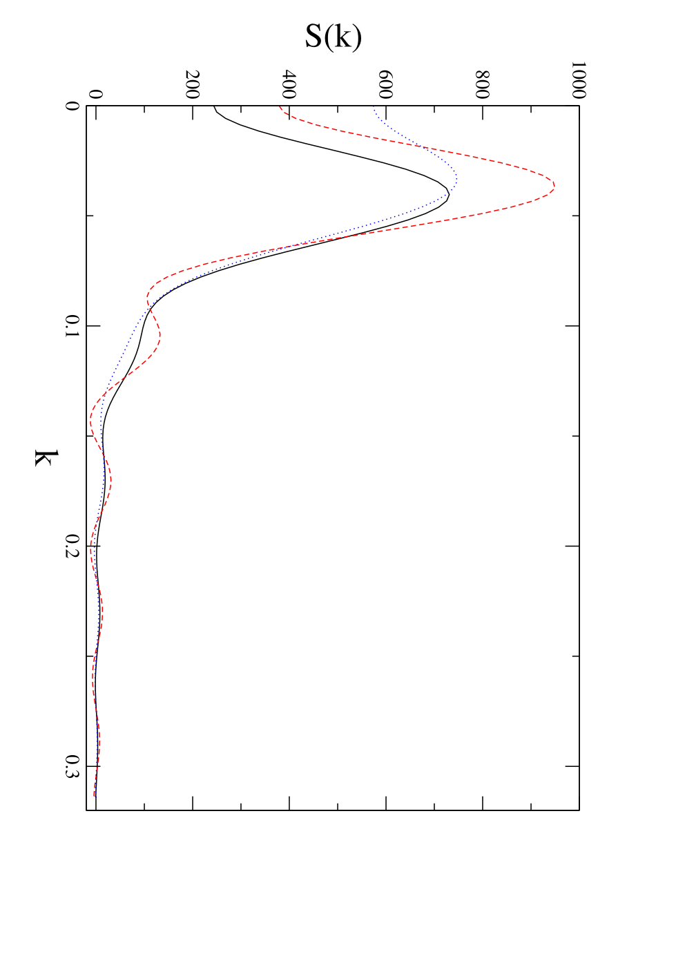
The Fourier space correlation functions can be found using Eqs. (9), (11) and are shown in Figs. 8 and 9. The spectra are dominated by peaks at . This corresponds to a length scale . From Fig. 4 we see that most sphalerons were nucleated at and these would primarily be on bubbles that are also of size , since most bubbles are nucleated at the earliest times. Hence the peak of the correlation is given by the sizes of the bubbles when bubbles started to percolate. The width of the peaks in Figs. 8 and 9 are and also given by the bubble sizes at percolation. Note that it would not be suitable to characterize the injected spectra by power law fits.

IV Conclusions and Future Directions
Following the general scenarios discussed in Refs. [1, 2] we have proposed a concrete model for the generation of helical magnetic fields during baryogenesis at a phase transition. The model takes into account magnetic field generation due to baryon number violating processes occurring on bubble walls. By Monte Carlo simulations, we have evaluated correlation functions of the injected magnetic field on completion of the phase transition. The Fourier space power spectra shown in Figs. 8 and 9 tell us the characteristics of the magnetic fields injected into the plasma in this model.
Our results should be viewed as providing initial conditions for subsequent evolution which will also entail MHD and cosmological effects. If the cosmological fluid is turbulent, say due to the motion of bubble walls, that too will play a role. These effects did not enter our study because the magnetic fields that are produced due to sphaleron events are on scales comparable to the inverse W-boson mass and far smaller than the scale at which the medium can be treated like a fluid. The micrscopic production, however, occurs at a high rate, since it is also the rate at which baryons are produced, and the magnetic field due to different sphalerons will subsequently spread, merge and permeate space.
MHD effects will come into play on length scales that are large compared to the thermal scale. As the magnetic field expands to larger scales, but still less than the frozen-in scale, MHD effects will change the linear expansion to diffusive expansion. On yet larger scales, the magnetic field expansion enters the frozen-in regime where it can only scale with the expansion of the universe. In addition to these considerations, the evolution needs to include the helicity of the magnetic field and any turbulence that may accompany the phase transition. It is known that helicity can be responsible for an “inverse cascade” that transfers power to larger scales. A discussion of some of these issues in the present context may be found in Ref. [2].
A long term goal of our model for generation of magnetic fields, is to connect the particle physics processes during baryogenesis (such as the phase transition) to characteristics of the magnetic field. The hope is that eventually the observation of a primordial magnetic field may say something about particle physics at the baryogenesis scale, the nano-second universe, and perhaps also the observed astrophysical magnetic structures.
Acknowledgements.
This work was supported by the U.S. Department of Energy at Case Western Reserve University. TV was also supported by grant number DE-FG02-90ER40542 at the Institute for Advanced Study.References
- [1] J. M. Cornwall, Phys. Rev. D 56, 6146 (1997) [arXiv:hep-th/9704022].
- [2] T. Vachaspati, Phys. Rev. Lett. 87, 251302 (2001) [arXiv:astro-ph/0101261].
- [3] N. S. Manton, Phys. Rev. D 28, 2019 (1983).
- [4] F. R. Klinkhamer and N. S. Manton, Phys. Rev. D 30, 2212 (1984).
- [5] C. H. Taubes, Commun. Math. Phys. 86, 257 (1982).
- [6] T. Vachaspati and G. B. Field, Phys. Rev. Lett. 73, 373 (1994) [arXiv:hep-ph/9401220].
- [7] M. Hindmarsh and M. James, Phys. Rev. D 49, 6109 (1994) [arXiv:hep-ph/9307205].
- [8] T. Vachaspati, “Kinks and domain walls: An introduction to classical and quantum solitons,” Cambridge, UK: Univ. Pr. (2006) 176 p
- [9] C. J. Copi, F. Ferrer, T. Vachaspati and A. Achucarro, Phys. Rev. Lett. 101, 171302 (2008) [arXiv:0801.3653 [astro-ph]].
- [10] S. Davidson, E. Nardi and Y. Nir, Phys. Rept. 466, 105 (2008) [arXiv:0802.2962 [hep-ph]].
- [11] “Classical Electrodynamics”, J. D. Jackson, Third Edition, Wiley (1998).
- [12] J. M. Cline, arXiv:hep-ph/0609145.
- [13] D. Bodeker and G. D. Moore, JCAP 0905, 009 (2009) [arXiv:0903.4099 [hep-ph]].
- [14] J. R. Espinosa, T. Konstandin, J. M. No and G. Servant, arXiv:1004.4187 [hep-ph].