跳到论文正文
W Papers独立论文阅读器 arXiv:1001.4693 论文正文 计算阅读时间 · 0%
引用这篇论文根据当前论文元数据生成,正式投稿前建议核对。


License: arXiv.org perpetual non-exclusive license
arXiv:1001.4693v3 [hep-ph] 04 Jun 2010

Analysis of the 12+{1\over 2}^{+} doubly heavy baryon states with QCD sum rules

Zhi-Gang Wang 11 1 E-mail,wangzgyiti@yahoo.com.cn.

Department of Physics, North China Electric Power University, Baoding 071003, P. R. China

PACS number: 14.20.Lq, 14.20.Mr

Key words: Heavy baryon states, QCD sum rules

Abstract

In this article, we study the 12+{1\over 2}^{+} doubly heavy baryon states ΩQ​Q\Omega_{QQ} and ΞQ​Q\Xi_{QQ} by subtracting the contributions from the corresponding 12−{1\over 2}^{-} doubly heavy baryon states with the QCD sum rules, and make reasonable predictions for their masses. Those doubly heavy baryon states maybe observed at the Tevatron, the LHCb and the PANDA.

1 Introduction

In 2002, the SELEX collaboration reported the first observation of a signal for the doubly charmed baryon state Ξc​c+\Xi_{cc}^{+} in the charged decay mode Ξc​c+→Λc+​K−​π+\Xi_{cc}^{+}\rightarrow\Lambda_{c}^{+}K^{-}\pi^{+} [1], and confirmed later by the same collaboration in the decay mode Ξc​c+→p​D+​K−\Xi_{cc}^{+}\rightarrow pD^{+}K^{-} with the measured mass MΞ=(3518.9±0.9)​MeVM_{\Xi}=(3518.9\pm 0.9)\,\rm{MeV} [2]. However, the Babar and Belle collaborations have not observed any evidence for the doubly charmed baryons in e+​e−e^{+}e^{-} annihilations [3, 4]. The charmed and bottom baryons which contain one (two) heavy quark(s) are particularly interesting for studying dynamics of the light quarks in the presence of the heavy quark(s), and serve as an excellent ground for testing predictions of the quark models and heavy quark symmetry. There have been several approaches to deal with the doubly heavy baryon masses, such as the relativistic quark model [5, 6], the non-relativistic quark model [7, 8, 9, 10], the three-body Faddeev method [11], the potential approach combined with the QCD sum rules [12], the quark model with AdS/QCD inspired potential [13], the MIT bag model [14], the full QCD sum rules [15, 16], and the Feynman-Hellmann theorem and semiempirical mass formulas [17], etc.

The QCD sum rules is a powerful theoretical tool in studying the ground state heavy baryons [18, 19, 20]. In the QCD sum rules, the operator product expansion is used to expand the time-ordered currents into a series of quark and gluon condensates which parameterize the long distance properties of the QCD vacuum. Based on the quark-hadron duality, we can obtain copious information about the hadronic parameters at the phenomenological side [18, 19]. There have been several works on the masses of the heavy baryon states with the full QCD sum rules and the QCD sum rules in the heavy quark effective theory (one can consult Ref.[21] for more literatures).

In Ref.[22], Jido et al introduce a novel approach based on the QCD sum rules to separate the contributions of the negative parity light flavor baryon states from the positive parity light flavor baryon states, as the interpolating currents may have non-vanishing couplings to both the negative parity and positive parity baryon states [23]. Before the work of Jido et al, Bagan et al take the infinite mass limit for the heavy quarks to separate the contributions of the positive parity and negative parity heavy baryon states unambiguously [24].

In Refs.[25, 26, 27], we study the heavy baryon states ΩQ\Omega_{Q}, ΞQ′\Xi^{\prime}_{Q}, ΣQ\Sigma_{Q}, ΩQ∗\Omega_{Q}^{*}, ΞQ∗\Xi^{*}_{Q} and ΣQ∗\Sigma^{*}_{Q} with the full QCD sum rules, and observe that the pole residues of the 32+{\frac{3}{2}}^{+} heavy baryon states from the sum rules with different tensor structures are consistent with each other, while the pole residues of the 12+{\frac{1}{2}}^{+} heavy baryon states from the sum rules with different tensor structures differ from each other greatly. In Refs.[21, 28], we follow Ref.[22] and study the masses and pole residues of the 12+{\frac{1}{2}}^{+} heavy baryon states ΩQ\Omega_{Q}, ΞQ′\Xi^{\prime}_{Q}, ΣQ\Sigma_{Q}, ΛQ\Lambda_{Q} and ΞQ\Xi_{Q} by subtracting the contributions of the negative parity heavy baryon states to overcome the embarrassment. Those pole residues are important parameters in studying the radiative decays ΩQ∗→ΩQ​γ\Omega_{Q}^{*}\to\Omega_{Q}\gamma, ΞQ∗→ΞQ′​γ\Xi_{Q}^{*}\to\Xi^{\prime}_{Q}\gamma and ΣQ∗→ΣQ​γ\Sigma_{Q}^{*}\to\Sigma_{Q}\gamma [27, 29], etc.

In this article, we extend our previous works to study the 12+{1\over 2}^{+} doubly heavy baryon states ΞQ​Q\Xi_{QQ} and ΩQ​Q\Omega_{QQ} with the QCD sum rules.

The article is arranged as follows: we derive the QCD sum rules for the masses and the pole residues of the doubly heavy baryon states ΞQ​Q\Xi_{QQ} and ΩQ​Q\Omega_{QQ} in Sec.2; in Sec.3, we present the numerical results and discussions; and Sec.4 is reserved for our conclusions.

2 QCD sum rules for the ΞQ​Q\Xi_{QQ} and ΩQ​Q\Omega_{QQ}

The 12+{1\over 2}^{+} doubly heavy baryon states ΞQ​Q\Xi_{QQ} and ΩQ​Q\Omega_{QQ} can be interpolated by the following currents JΞ​(x)J_{\Xi}(x) and JΩ​(x)J_{\Omega}(x) respectively,

JΞ​(x)\displaystyle J_{\Xi}(x) =\displaystyle= ϵi​j​k​QiT​(x)​C​γμ​Qj​(x)​γ5​γμ​qk​(x),\displaystyle\epsilon^{ijk}Q^{T}_{i}(x)C\gamma_{\mu}Q_{j}(x)\gamma_{5}\gamma^{\mu}q_{k}(x)\,,
JΩ​(x)\displaystyle J_{\Omega}(x) =\displaystyle= ϵi​j​k​QiT​(x)​C​γμ​Qj​(x)​γ5​γμ​sk​(x),\displaystyle\epsilon^{ijk}Q^{T}_{i}(x)C\gamma_{\mu}Q_{j}(x)\gamma_{5}\gamma^{\mu}s_{k}(x)\,, (1)

where the QQ represents the heavy quarks cc and bb, the ii, jj and kk are color indexes, and the CC is the charge conjunction matrix. In the heavy quark limit, the doubly heavy baryon states can be described by the (heavy)diquark-(light)quark model [12].

The corresponding 12−{1\over 2}^{-} doubly heavy baryon states can be interpolated by the currents J−=i​γ5​J+J_{-}=i\gamma_{5}J_{+} because multiplying i​γ5i\gamma_{5} to J+J_{+} changes the parity of J+J_{+} [22], where the J+J_{+} denotes the currents JΩ​(x)J_{\Omega}(x) and JΞ​(x)J_{\Xi}(x). The correlation functions are defined by

Π±​(p)\displaystyle\Pi_{\pm}(p) =\displaystyle= i​∫d4​x​ei​p⋅x​⟨0|T⁡{J±​(x)​J¯±​(0)}|0⟩,\displaystyle i\int d^{4}xe^{ip\cdot x}\langle 0|T\left\{J_{\pm}(x)\bar{J}_{\pm}(0)\right\}|0\rangle\,, (2)

and can be decomposed as

Π±​(p)=​p​Π1​(p2)±Π0​(p2),\Pi_{\pm}(p)=\!\not\!{p}\Pi_{1}(p^{2})\pm\Pi_{0}(p^{2})\,, (3)

due to Lorentz covariance. The currents J+J_{+} couple to both the positive parity and negative parity baryon states [23], i.e. ⟨0|J+|B−⟩​⟨B−|J¯+|0⟩=−γ5​⟨0​|J−​|B−⟩​⟨B−|​J¯−|​0⟩​γ5\langle{0}|J_{+}|B^{-}\rangle\langle B^{-}|\bar{J}_{+}|0\rangle=-\gamma_{5}\langle 0|J_{-}|B^{-}\rangle\langle B^{-}|\bar{J}_{-}|0\rangle\gamma_{5}, where the B−B^{-} denote the negative parity baryon states.

We insert a complete set of intermediate baryon states with the same quantum numbers as the current operators J+​(x)J_{+}(x) and J−​(x)J_{-}(x) into the correlation functions Π+​(p)\Pi_{+}(p) to obtain the hadronic representation [18, 19]. After isolating the pole terms of the lowest states of the doubly heavy baryons, we obtain the following result [22]:

Π+​(p)\displaystyle\Pi_{+}(p) =\displaystyle= λ+2​​p+M+M+2−p2+λ−2​​p−M−M−2−p2+⋯,\displaystyle\lambda_{+}^{2}{\!\not\!{p}+M_{+}\over M^{2}_{+}-p^{2}}+\lambda_{-}^{2}{\!\not\!{p}-M_{-}\over M_{-}^{2}-p^{2}}+\cdots\,, (4)

where the M±M_{\pm} are the masses of the lowest states with parity ±\pm respectively, and the λ±\lambda_{\pm} are the corresponding pole residues (or couplings). If we take p→=0\vec{p}=0, then

limitϵ→0​Im​Π+​(p0+i​ϵ)π\displaystyle\rm{limit}_{\epsilon\rightarrow 0}\frac{{\rm Im}\Pi_{+}(p_{0}+i\epsilon)}{\pi} =\displaystyle= λ+2​γ0+12​δ​(p0−M+)+λ−2​γ0−12​δ​(p0−M−)+⋯\displaystyle\lambda_{+}^{2}{\gamma_{0}+1\over 2}\delta(p_{0}-M_{+})+\lambda_{-}^{2}{\gamma_{0}-1\over 2}\delta(p_{0}-M_{-})+\cdots (5)
=\displaystyle= γ0​A​(p0)+B⁡(p0)+⋯,\displaystyle\gamma_{0}A(p_{0})+B(p_{0})+\cdots\,,

where

A⁡(p0)\displaystyle A(p_{0}) =\displaystyle= 12​[λ+2​δ​(p0−M+)+λ−2​δ​(p0−M−)],\displaystyle{1\over 2}\left[\lambda_{+}^{2}\delta(p_{0}-M_{+})+\lambda_{-}^{2}\delta(p_{0}-M_{-})\right]\,,
B⁡(p0)\displaystyle B(p_{0}) =\displaystyle= 12​[λ+2​δ​(p0−M+)−λ−2​δ​(p0−M−)],\displaystyle{1\over 2}\left[\lambda_{+}^{2}\delta(p_{0}-M_{+})-\lambda_{-}^{2}\delta(p_{0}-M_{-})\right]\,, (6)

the A⁡(p0)+B⁡(p0)A(p_{0})+B(p_{0}) and A⁡(p0)−B⁡(p0)A(p_{0})-B(p_{0}) contain the contributions from the positive-parity and negative-parity baryon states respectively.

We calculate the light quark parts of the correlation functions Π+​(p)\Pi_{+}(p) in the coordinate space and use the momentum space expression for the heavy quark propagators, i.e. we take

Si​j​(x)\displaystyle S_{ij}(x) =\displaystyle= i​δi​j​​x2​π2​x4−δi​j​ms4​π2​x2−δi​j12​⟨s¯​s⟩+i​δi​j48​ms​⟨s¯​s⟩​​x\displaystyle\frac{i\delta_{ij}\!\not\!{x}}{2\pi^{2}x^{4}}-\frac{\delta_{ij}m_{s}}{4\pi^{2}x^{2}}-\frac{\delta_{ij}}{12}\langle\bar{s}s\rangle+\frac{i\delta_{ij}}{48}m_{s}\langle\bar{s}s\rangle\!\not\!{x}
−i32​π2​x2​Gμ​νi​j​(x)​[​x​σμ​ν+σμ​ν​​x]+⋯,\displaystyle-\frac{i}{32\pi^{2}x^{2}}G^{ij}_{\mu\nu}(x)\left[\!\not\!{x}\sigma^{\mu\nu}+\sigma^{\mu\nu}\!\not\!{x}\right]+\cdots\,,
SQi​j​(x)\displaystyle S_{Q}^{ij}(x) =\displaystyle= i(2​π)4∫d4ke−ik⋅x{δi​j​k−mQ−gs​Gi​jα​β4σα​β​(​k+mQ)+(​k+mQ)​σα​β(k2−mQ2)2\displaystyle\frac{i}{(2\pi)^{4}}\int d^{4}ke^{-ik\cdot x}\left\{\frac{\delta_{ij}}{\!\not\!{k}-m_{Q}}-\frac{g_{s}G^{\alpha\beta}_{ij}}{4}\frac{\sigma_{\alpha\beta}(\!\not\!{k}+m_{Q})+(\!\not\!{k}+m_{Q})\sigma_{\alpha\beta}}{(k^{2}-m_{Q}^{2})^{2}}\right. (7)
+π23⟨αs​G​Gπ⟩δi​jmQk2+mQ​​k(k2−mQ2)4+⋯},\displaystyle\left.+\frac{\pi^{2}}{3}\langle\frac{\alpha_{s}GG}{\pi}\rangle\delta_{ij}m_{Q}\frac{k^{2}+m_{Q}\!\not\!{k}}{(k^{2}-m_{Q}^{2})^{4}}+\cdots\right\}\,,

where ⟨αs​G​Gπ⟩=⟨αs​Gα​β​Gα​βπ⟩\langle\frac{\alpha_{s}GG}{\pi}\rangle=\langle\frac{\alpha_{s}G_{\alpha\beta}G^{\alpha\beta}}{\pi}\rangle, then resort to the Fourier integral to transform the light quark parts into the momentum space in DD dimensions, take p→=0\vec{p}=0, and use the dispersion relation to obtain the spectral densities ρA​(p0)\rho^{A}(p_{0}) and ρB​(p0)\rho^{B}(p_{0}) (which correspond to the tensor structures γ0\gamma_{0} and 11 respectively) at the level of quark-gluon degrees of freedom. Finally we introduce the weight functions exp⁡[−p02T2]\exp\left[-\frac{p_{0}^{2}}{T^{2}}\right], p02​exp⁡[−p02T2]p_{0}^{2}\exp\left[-\frac{p_{0}^{2}}{T^{2}}\right], and obtain the following sum rules,

λ+2​exp⁡[−M+2T2]\displaystyle\lambda_{+}^{2}\exp\left[-\frac{M_{+}^{2}}{T^{2}}\right] =\displaystyle= ∫Δs0d​p0​[ρA​(p0)+ρB​(p0)]​exp⁡[−p02T2],\displaystyle\int_{\Delta}^{\sqrt{s_{0}}}dp_{0}\left[\rho^{A}(p_{0})+\rho^{B}(p_{0})\right]\exp\left[-\frac{p_{0}^{2}}{T^{2}}\right]\,, (8)
λ+2​M+2​exp⁡[−M+2T2]\displaystyle\lambda_{+}^{2}M_{+}^{2}\exp\left[-\frac{M_{+}^{2}}{T^{2}}\right] =\displaystyle= ∫Δs0d​p0​[ρA​(p0)+ρB​(p0)]​p02​exp⁡[−p02T2],\displaystyle\int_{\Delta}^{\sqrt{s_{0}}}dp_{0}\left[\rho^{A}(p_{0})+\rho^{B}(p_{0})\right]p_{0}^{2}\exp\left[-\frac{p_{0}^{2}}{T^{2}}\right]\,, (9)

where

ρΩA​(p0)\displaystyle\rho^{A}_{\Omega}(p_{0}) =\displaystyle= 3​p08​π4​∫αiαfd​α​∫βi1−αd​β​α​β​(1−α−β)​(p02−m~Q2)​(5​p02−3​m~Q2)\displaystyle\frac{3p_{0}}{8\pi^{4}}\int_{\alpha_{i}}^{\alpha_{f}}d\alpha\int_{\beta_{i}}^{1-\alpha}d\beta\alpha\beta(1-\alpha-\beta)(p_{0}^{2}-\widetilde{m}^{2}_{Q})(5p_{0}^{2}-3\widetilde{m}^{2}_{Q}) (10)
+3​mQ2​p08​π4∫αiαfdα∫βi1−αdβ(1−α−β)(p02−m~Q2)\displaystyle+\frac{3m_{Q}^{2}p_{0}}{8\pi^{4}}\int_{\alpha_{i}}^{\alpha_{f}}d\alpha\int_{\beta_{i}}^{1-\alpha}d\beta(1-\alpha-\beta)(p_{0}^{2}-\widetilde{m}^{2}_{Q})
−mQ224​π2⟨αs​G​Gπ⟩∫αiαfdα∫βi1−αdβ(1−α−β)[αβ2+βα2][1+p04​T]δ(p0−m~Q)\displaystyle-\frac{m_{Q}^{2}}{24\pi^{2}}\langle\frac{\alpha_{s}GG}{\pi}\rangle\int_{\alpha_{i}}^{\alpha_{f}}d\alpha\int_{\beta_{i}}^{1-\alpha}d\beta(1-\alpha-\beta)\left[\frac{\alpha}{\beta^{2}}+\frac{\beta}{\alpha^{2}}\right]\left[1+\frac{p_{0}}{4T}\right]\delta(p_{0}-\widetilde{m}_{Q})
−mQ4192​π2​p0​T⟨αs​G​Gπ⟩∫αiαfdα∫βi1−αdβ(1−α−β)[1α3+1β3]δ(p0−m~Q)\displaystyle-\frac{m_{Q}^{4}}{192\pi^{2}p_{0}T}\langle\frac{\alpha_{s}GG}{\pi}\rangle\int_{\alpha_{i}}^{\alpha_{f}}d\alpha\int_{\beta_{i}}^{1-\alpha}d\beta(1-\alpha-\beta)\left[\frac{1}{\alpha^{3}}+\frac{1}{\beta^{3}}\right]\delta(p_{0}-\widetilde{m}_{Q})
+mQ232​π2⟨αs​G​Gπ⟩∫αiαfdα∫βi1−αdβ(1−α−β)[1α2+1β2]δ(p0−m~Q)\displaystyle+\frac{m_{Q}^{2}}{32\pi^{2}}\langle\frac{\alpha_{s}GG}{\pi}\rangle\int_{\alpha_{i}}^{\alpha_{f}}d\alpha\int_{\beta_{i}}^{1-\alpha}d\beta(1-\alpha-\beta)\left[\frac{1}{\alpha^{2}}+\frac{1}{\beta^{2}}\right]\delta(p_{0}-\widetilde{m}_{Q})
+ms​⟨s¯​s⟩4​π2∫αiαfdαα(1−α)[6p0+p02δ(p0−m~~Q)]\displaystyle+\frac{m_{s}\langle\bar{s}{s}\rangle}{4\pi^{2}}\int_{\alpha_{i}}^{\alpha_{f}}d\alpha\alpha(1-\alpha)\left[6p_{0}+p_{0}^{2}\delta(p_{0}-\widetilde{\widetilde{m}}_{Q})\right]
+ms​mQ2​⟨s¯​s⟩8​π2∫αiαfdαδ(p0−m~~Q)\displaystyle+\frac{m_{s}m_{Q}^{2}\langle\bar{s}{s}\rangle}{8\pi^{2}}\int_{\alpha_{i}}^{\alpha_{f}}d\alpha\delta(p_{0}-\widetilde{\widetilde{m}}_{Q})
+132​π2⟨αs​G​Gπ⟩∫αiαfdα∫βi1−αdβ(α+β)[3p0+m~Q22δ(p0−m~Q)]\displaystyle+\frac{1}{32\pi^{2}}\langle\frac{\alpha_{s}GG}{\pi}\rangle\int_{\alpha_{i}}^{\alpha_{f}}d\alpha\int_{\beta_{i}}^{1-\alpha}d\beta(\alpha+\beta)\left[3p_{0}+\frac{\widetilde{m}_{Q}^{2}}{2}\delta(p_{0}-\widetilde{m}_{Q})\right]
+mQ264​π2⟨αs​G​Gπ⟩∫αiαfdα∫βi1−αdβα+βα​βδ(p0−m~Q),\displaystyle+\frac{m_{Q}^{2}}{64\pi^{2}}\langle\frac{\alpha_{s}GG}{\pi}\rangle\int_{\alpha_{i}}^{\alpha_{f}}d\alpha\int_{\beta_{i}}^{1-\alpha}d\beta\frac{\alpha+\beta}{\alpha\beta}\delta(p_{0}-\widetilde{m}_{Q})\,,
ρΩB​(p0)\displaystyle\rho^{B}_{\Omega}(p_{0}) =\displaystyle= 3​ms8​π4​∫αiαfd​α​∫βi1−αd​β​α​β​(p02−m~Q2)​(2​p02−m~Q2)\displaystyle\frac{3m_{s}}{8\pi^{4}}\int_{\alpha_{i}}^{\alpha_{f}}d\alpha\int_{\beta_{i}}^{1-\alpha}d\beta\alpha\beta(p_{0}^{2}-\widetilde{m}^{2}_{Q})(2p_{0}^{2}-\widetilde{m}^{2}_{Q}) (11)
+3​ms​mQ24​π4∫αiαfdα∫βi1−αdβ(p02−m~Q2)\displaystyle+\frac{3m_{s}m_{Q}^{2}}{4\pi^{4}}\int_{\alpha_{i}}^{\alpha_{f}}d\alpha\int_{\beta_{i}}^{1-\alpha}d\beta(p_{0}^{2}-\widetilde{m}^{2}_{Q})
−ms​mQ296​π2⟨αs​G​Gπ⟩∫αiαfdα∫βi1−αdβ[αβ2+βα2][1m~Q+12​T]δ(p0−m~Q)\displaystyle-\frac{m_{s}m_{Q}^{2}}{96\pi^{2}}\langle\frac{\alpha_{s}GG}{\pi}\rangle\int_{\alpha_{i}}^{\alpha_{f}}d\alpha\int_{\beta_{i}}^{1-\alpha}d\beta\left[\frac{\alpha}{\beta^{2}}+\frac{\beta}{\alpha^{2}}\right]\left[\frac{1}{\widetilde{m}_{Q}}+\frac{1}{2T}\right]\delta(p_{0}-\widetilde{m}_{Q})
−ms​mQ496​π2​p02​T⟨αs​G​Gπ⟩∫αiαfdα∫βi1−αdβ[1α3+1β3]δ(p0−m~Q)\displaystyle-\frac{m_{s}m_{Q}^{4}}{96\pi^{2}p_{0}^{2}T}\langle\frac{\alpha_{s}GG}{\pi}\rangle\int_{\alpha_{i}}^{\alpha_{f}}d\alpha\int_{\beta_{i}}^{1-\alpha}d\beta\left[\frac{1}{\alpha^{3}}+\frac{1}{\beta^{3}}\right]\delta(p_{0}-\widetilde{m}_{Q})
+ms​mQ216​π2​p0⟨αs​G​Gπ⟩∫αiαfdα∫βi1−αdβ[1α2+1β2]δ(p0−m~Q)\displaystyle+\frac{m_{s}m_{Q}^{2}}{16\pi^{2}p_{0}}\langle\frac{\alpha_{s}GG}{\pi}\rangle\int_{\alpha_{i}}^{\alpha_{f}}d\alpha\int_{\beta_{i}}^{1-\alpha}d\beta\left[\frac{1}{\alpha^{2}}+\frac{1}{\beta^{2}}\right]\delta(p_{0}-\widetilde{m}_{Q})
−⟨s¯​s⟩2​π2∫αiαfdαα(1−α)[3p02−2m~~Q2]−mQ2​⟨s¯​s⟩π2∫αiαfdα\displaystyle-\frac{\langle\bar{s}{s}\rangle}{2\pi^{2}}\int_{\alpha_{i}}^{\alpha_{f}}d\alpha\alpha(1-\alpha)\left[3p_{0}^{2}-2\widetilde{\widetilde{m}}_{Q}^{2}\right]-\frac{m_{Q}^{2}\langle\bar{s}{s}\rangle}{\pi^{2}}\int_{\alpha_{i}}^{\alpha_{f}}d\alpha
−ms16​π2⟨αs​G​Gπ⟩∫αiαfdα∫βi1−αdβ[1+m~Q4δ(p0−m~Q)],\displaystyle-\frac{m_{s}}{16\pi^{2}}\langle\frac{\alpha_{s}GG}{\pi}\rangle\int_{\alpha_{i}}^{\alpha_{f}}d\alpha\int_{\beta_{i}}^{1-\alpha}d\beta\left[1+\frac{\widetilde{m}_{Q}}{4}\delta(p_{0}-\widetilde{m}_{Q})\right]\,,

the s0s_{0} are the threshold parameters, T2T^{2} are the Borel parameters, αf=1+1−4​mQ2/p022\alpha_{f}=\frac{1+\sqrt{1-4m_{Q}^{2}/p_{0}^{2}}}{2}, αi=1−1−4​mQ2/p022\alpha_{i}=\frac{1-\sqrt{1-4m_{Q}^{2}/p_{0}^{2}}}{2}, βi=α​mQ2α​p02−mQ2\beta_{i}=\frac{\alpha m_{Q}^{2}}{\alpha p_{0}^{2}-m_{Q}^{2}}, m~Q2=(α+β)​mQ2α​β\widetilde{m}_{Q}^{2}=\frac{(\alpha+\beta)m_{Q}^{2}}{\alpha\beta}, m~~Q2=mQ2α⁡(1−α)\widetilde{\widetilde{m}}_{Q}^{2}=\frac{m_{Q}^{2}}{\alpha(1-\alpha)}, and Δ=2​mQ+ms\Delta=2m_{Q}+m_{s}. With the simple replacements, ⟨s¯​s⟩→⟨q¯​q⟩\langle\bar{s}s\rangle\rightarrow\langle\bar{q}q\rangle and ms→0m_{s}\rightarrow 0, we can obtain the corresponding spectral densities of the ΞQ​Q\Xi_{QQ} at the level of quark-gluon degrees of freedom.

3 Numerical results and discussions

The input parameters are taken as ⟨q¯​q⟩=−(0.24±0.01​GeV)3\langle\bar{q}q\rangle=-(0.24\pm 0.01\,\rm{GeV})^{3}, ⟨s¯​s⟩=(0.8±0.2)​⟨q¯​q⟩\langle\bar{s}s\rangle=(0.8\pm 0.2)\langle\bar{q}q\rangle, ⟨q¯​gs​σ​G​q⟩=m02​⟨q¯​q⟩\langle\bar{q}g_{s}\sigma Gq\rangle=m_{0}^{2}\langle\bar{q}q\rangle, ⟨s¯​gs​σ​G​s⟩=m02​⟨s¯​s⟩\langle\bar{s}g_{s}\sigma Gs\rangle=m_{0}^{2}\langle\bar{s}s\rangle, m02=(0.8±0.2)​GeV2m_{0}^{2}=(0.8\pm 0.2)\,\rm{GeV}^{2} [30, 31], ⟨αs​G​Gπ⟩=(0.012±0.004)​GeV4\langle\frac{\alpha_{s}GG}{\pi}\rangle=(0.012\pm 0.004)\,\rm{GeV}^{4} [31], ms=(0.14±0.01)​GeVm_{s}=(0.14\pm 0.01)\,\rm{GeV}, mc=(1.35±0.10)​GeVm_{c}=(1.35\pm 0.10)\,\rm{GeV} and mb=(4.7±0.1)​GeVm_{b}=(4.7\pm 0.1)\,\rm{GeV} [32] at the energy scale μ=1​GeV\mu=1\,\rm{GeV}.

The value of the gluon condensate ⟨αs​G​Gπ⟩\langle\frac{\alpha_{s}GG}{\pi}\rangle has been updated from time to time, and changes greatly [20]. At the present case, the gluon condensate makes tiny contribution (see Table 1), the updated value ⟨αs​G​Gπ⟩=(0.023±0.003)​GeV4\langle\frac{\alpha_{s}GG}{\pi}\rangle=(0.023\pm 0.003)\,\rm{GeV}^{4} [20] and the standard value ⟨αs​G​Gπ⟩=(0.012±0.004)​GeV4\langle\frac{\alpha_{s}GG}{\pi}\rangle=(0.012\pm 0.004)\,\rm{GeV}^{4} [31] lead to a slight difference and can be neglected safely.

The QQ-quark masses appearing in the perturbative terms are usually taken to be the pole masses in the QCD sum rules, while the choice of the mQm_{Q} in the leading-order coefficients of the higher-dimensional terms is arbitrary [20, 33]. The M​S¯\overline{MS} mass mc​(mc2)m_{c}(m_{c}^{2}) relates with the pole mass m^c\hat{m}_{c} through the relation mc​(mc2)=m^c​[1+CF​αs​(mc2)π+⋯]−1m_{c}(m_{c}^{2})=\hat{m}_{c}\left[1+\frac{C_{F}\alpha_{s}(m_{c}^{2})}{\pi}+\cdots\right]^{-1}. In this article, we take the approximation mc​(mc2)≈m^cm_{c}(m_{c}^{2})\approx\hat{m}_{c} without the αs\alpha_{s} corrections for consistency. The value listed in the Particle Data Group is mc​(mc2)=1.27−0.11+0.07​GeVm_{c}(m_{c}^{2})=1.27^{+0.07}_{-0.11}\,\rm{GeV} [32], it is reasonable to take m^c=mc​(1​GeV2)=(1.35±0.10)​GeV\hat{m}_{c}=m_{c}(1\,\rm{GeV}^{2})=(1.35\pm 0.10)\,\rm{GeV}. For the bb quark, the M​S¯\overline{MS} mass mb​(mb2)=4.20−0.07+0.17​GeVm_{b}(m_{b}^{2})=4.20^{+0.17}_{-0.07}\,\rm{GeV} [32], the gap between the energy scale μ=4.2​GeV\mu=4.2\,\rm{GeV} and 1​GeV1\,\rm{GeV} is rather large, the approximation m^b≈mb​(mb2)≈mb​(1​GeV2)\hat{m}_{b}\approx m_{b}(m_{b}^{2})\approx m_{b}(1\,\rm{GeV}^{2}) seems rather crude. It would be better to understand the quark masses mcm_{c} and mbm_{b} we take at the energy scale μ2=1​GeV2\mu^{2}=1\,\rm{GeV}^{2} as the effective quark masses (or just the mass parameters).

In calculation, we neglect the contributions from the perturbative 𝒪⁡(αsn)\mathcal{O}(\alpha_{s}^{n}) corrections. Those perturbative corrections can be taken into account in the leading logarithmic approximations through the anomalous dimension factors. After the Borel transform, the effects of those corrections are to multiply each term on the operator product expansion side by the factor, [αs​(T2)αs​(μ2)]2​ΓJ−Γ𝒪n\left[\frac{\alpha_{s}(T^{2})}{\alpha_{s}(\mu^{2})}\right]^{2\Gamma_{J}-\Gamma_{\mathcal{O}_{n}}}, where the ΓJ\Gamma_{J} is the anomalous dimension of the interpolating current J⁡(x)J(x), and the Γ𝒪n\Gamma_{\mathcal{O}_{n}} is the anomalous dimension of the local operator 𝒪n​(0)\mathcal{O}_{n}(0), which governs the evolution of the vacuum condensate ⟨On​(0)⟩μ\langle{O}_{n}(0)\rangle_{\mu} with the energy scale through the renormalization group equation.

If the perturbative 𝒪⁡(αs)\mathcal{O}(\alpha_{s}) corrections and the anomalous dimension factors are taken into account consistently, the spectral densities in the QCD side should be replaced with

𝒪0​(0)\displaystyle\mathcal{O}_{0}(0) →\displaystyle\rightarrow [αs​(T2)αs​(μ2)]2​ΓJ​[1+A⁡(p02,mQ2)​αs​(T2)π]​𝒪0​(0),\displaystyle\left[\frac{\alpha_{s}(T^{2})}{\alpha_{s}(\mu^{2})}\right]^{2\Gamma_{J}}\left[1+A(p_{0}^{2},m_{Q}^{2})\frac{\alpha_{s}(T^{2})}{\pi}\right]\mathcal{O}_{0}(0)\,,
⟨𝒪n​(0)⟩μ\displaystyle\langle\mathcal{O}_{n}(0)\rangle_{\mu} →\displaystyle\rightarrow [αs​(T2)αs​(μ2)]2​ΓJ−Γ𝒪n​[1+B⁡(p02,mQ2)​αs​(T2)π]​⟨𝒪n​(0)⟩μ,\displaystyle\left[\frac{\alpha_{s}(T^{2})}{\alpha_{s}(\mu^{2})}\right]^{2\Gamma_{J}-\Gamma_{\mathcal{O}_{n}}}\left[1+B(p_{0}^{2},m_{Q}^{2})\frac{\alpha_{s}(T^{2})}{\pi}\right]\langle\mathcal{O}_{n}(0)\rangle_{\mu}\,,

where the A⁡(p02,mQ2)A(p_{0}^{2},m_{Q}^{2}) and B⁡(p02,mQ2)B(p_{0}^{2},m_{Q}^{2}) are some notations for the coefficients of the perturbative corrections, the average virtuality of the quarks in the correlation functions is characterized by the Borel parameter T2T^{2}. We cannot estimate the corrections and the uncertainties originate from the corrections with confidence without explicit calculations. In the case of the correlation function for the proton, the perturbative 𝒪⁡(αs)\mathcal{O}(\alpha_{s}) corrections can change the numerical values of the mass and the pole residue considerably and improve the agreement between the theoretical estimation and the experimental data [30, 34]. In the present case, including the αs\alpha_{s} corrections maybe improve the predictions.

In this article, we carry out the operator product expansion at the special energy scale μ2=1​GeV2\mu^{2}=1\,\rm{GeV}^{2}, and set the factor [αs​(T2)αs​(μ2)]2​ΓJ−Γ𝒪n≈1\left[\frac{\alpha_{s}(T^{2})}{\alpha_{s}(\mu^{2})}\right]^{2\Gamma_{J}-\Gamma_{\mathcal{O}_{n}}}\approx 1 for consistency, as the αs\alpha_{s} corrections have not been calculated yet. Such an approximation maybe result in some scale dependence and weaken the prediction ability. In this article, we study the JP=12+J^{P}=\frac{1}{2}^{+} doubly heavy baryon states systemically, the predictions are reasonable as we take the analogous criteria in those sum rules.

In the conventional QCD sum rules [18, 19], there are two criteria (pole dominance and convergence of the operator product expansion) for choosing the Borel parameter T2T^{2} and threshold parameter s0s_{0}. We impose the two criteria on the doubly heavy baryon states to choose the Borel parameter T2T^{2} and threshold parameter s0s_{0}.

Refer to caption
Refer to caption
Refer to caption
Refer to caption
Figure 1: The contributions of the pole terms with variations of the Borel parameters T2T^{2}, the AA, BB, CC and DD correspond to the channels Ξc​c\Xi_{cc}, Ωc​c\Omega_{cc}, Ξb​b\Xi_{bb} and Ωb​b\Omega_{bb} respectively, the β\beta corresponds to the central values of the threshold parameters, the energy gap among α\alpha, β\beta and γ\gamma is 0.1​GeV0.1\,\rm{GeV}.

In Fig.1, we plot the contributions from the pole terms with variations of the Borel parameters T2T^{2} and the threshold parameters s0s_{0}. The pole contributions are larger than (or about) 50%50\% at the values which are denoted by the vertical lines for central values (β\beta) of the threshold parameters s0s_{0}. From the figure, we can set the upper bound of the Borel parameters Tm​a​x2T^{2}_{max}, Tm​a​x2=3.8​GeV2T^{2}_{max}=3.8\,\rm{GeV}^{2}, 4.0​GeV24.0\,\rm{GeV}^{2}, 9.1​GeV29.1\,\rm{GeV}^{2} and 9.3​GeV29.3\,\rm{GeV}^{2} in the channels Ξc​c\Xi_{cc}, Ωc​c\Omega_{cc}, Ξb​b\Xi_{bb} and Ωb​b\Omega_{bb}, respectively. The lower bound of the Borel parameters Tm​i​n2T^{2}_{min} can be determined in the regions where the contributions from the perturbative terms are larger than (or equal) the ones from the quark condensates, Tm​i​n2=2.8​GeV2T^{2}_{min}=2.8\,\rm{GeV}^{2}, 1.6​GeV21.6\,\rm{GeV}^{2}, 7.7​GeV27.7\,\rm{GeV}^{2} and <6.5​GeV2<6.5\,\rm{GeV}^{2} in the channels Ξc​c\Xi_{cc}, Ωc​c\Omega_{cc}, Ξb​b\Xi_{bb} and Ωb​b\Omega_{bb}, respectively. The convergent behaviors in the channels ΩQ​Q\Omega_{QQ} are better than the corresponding ones in the channels ΞQ​Q\Xi_{QQ}, this is mainly due to the fact that the values of the quark condensates, |⟨q¯​q⟩|>|⟨s¯​s⟩||\langle\bar{q}{q}\rangle|>|\langle\bar{s}{s}\rangle|. The Borel windows Tm​i​n2−Tm​a​x2T^{2}_{min}-T^{2}_{max} in the channels ΞQ​Q\Xi_{QQ} and ΩQ​Q\Omega_{QQ} overlap with each other. In this article, we can take the uniform intervals for the Borel windows (IBW), i.e. IBW=1.0​GeV2\rm{IBW}=1.0\,\rm{GeV}^{2} and 1.4​GeV21.4\,\rm{GeV}^{2} in the doubly charmed and doubly bottom channels respectively, which warrant the pole contributions are analogous. The values of the threshold parameters s0s_{0} and the Borel parameters T2T^{2} are shown in Table 1, from the table, we can see that the two criteria of the QCD sum rules are fully satisfied [18, 19].

In Ref.[21], we study the 12+{\frac{1}{2}}^{+} sextet heavy baryon states Ωb\Omega_{b}, Ωc\Omega_{c}, Ξb′\Xi^{\prime}_{b}, Ξc′\Xi^{\prime}_{c}, Σb\Sigma_{b} and Σc\Sigma_{c} by subtracting the contributions from the corresponding negative parity heavy baryon states with the QCD sum rules, the predicted masses are in good agreement with the experimental data for the well established mesons, Ωb\Omega_{b}, Σb\Sigma_{b}, Ωc\Omega_{c}, Ξc′\Xi^{\prime}_{c} and Σc\Sigma_{c}. In those sum rules, the contributions from the pole terms are about (45−65)%(45-65)\% and (45−80)%(45-80)\% for the bottom and charmed baryon states respectively. In this article, we take analogous pole contributions, see Table 1, the predictions are reasonable although the contributions from the perturbative continuum are somewhat large.

In Fig.2, we plot the predicted masses with variations of the threshold parameters s0s_{0}. From the figure, we can see that the predicted masses are not sensitive to the threshold parameters, although they increase with the threshold parameters. In calculation, we take uniform uncertainties for the threshold parameters, δs0=±0.1​GeV\delta_{\sqrt{s_{0}}}=\pm 0.1\,\rm{GeV}.

From Table 1, we can see that the contributions from the quark condensates are large, even comparable with the perturbative terms, this is an indication of the non-perturbative origin of the masses of the baryon states. In the chiral limit, the spectral densities on the QCD side come from the quark condensates only. An astonishingly simple expression can be obtained in case of the proton [35, 36],

Mp\displaystyle M_{p} =\displaystyle= −8​π2​⟨q¯​q⟩μ=1​GeV3≈1​GeV.\displaystyle\sqrt[3]{-8\pi^{2}\langle\bar{q}q\rangle_{\mu=1\,\rm{GeV}}}\approx 1\,\rm{GeV}\,. (12)

Taking into account all uncertainties of the relevant parameters, we can obtain the values of the masses and pole residues of the doubly heavy baryon states ΞQ​Q\Xi_{QQ} and ΩQ​Q\Omega_{QQ}, which are shown in Figs.3-4 and Tables 2-3. In Table 2, we also present the predictions of other theoretical approaches and the values of the experimental data, the present predictions are consistent with them.

T2​(GeV2)T^{2}(\rm{GeV}^{2}) s0​(GeV)\sqrt{s_{0}}(\rm{GeV}) pole perturbative ⟨q¯​q⟩\langle\bar{q}q\rangle ⟨αs​G​Gπ⟩\langle\frac{\alpha_{s}GG}{\pi}\rangle
Ξc​c\Xi_{cc} 2.8−3.82.8-3.8 4.24.2 (46−78)%(46-78)\% (48−55)%(48-55)\% (43−50)%(43-50)\% ≈2%\approx 2\%
Ωc​c\Omega_{cc} 3.0−4.03.0-4.0 4.34.3 (45−75)%(45-75)\% (67−72)%(67-72)\% (26−30)%(26-30)\% ≈2%\approx 2\%
Ξb​b\Xi_{bb} 7.7−9.17.7-9.1 10.810.8 (46−69)%(46-69)\% (48−53)%(48-53)\% (46−51)%(46-51)\% <1%<1\%
Ωb​b\Omega_{bb} 7.9−9.37.9-9.3 10.910.9 (46−68)%(46-68)\% (69−72)%(69-72)\% (28−31)%(28-31)\% <1%<1\%
Table 1: The Borel parameters T2T^{2} and threshold parameters s0s_{0} for the doubly heavy baryon states, the ”pole” stands for the contribution from the pole term, and the ”perturbative” stands for the contribution from the perturbative term in the operator product expansion, etc. In calculating the contributions from the pole terms, we take into account the uniform uncertainties of the threshold parameters, δs0=±0.1​GeV\delta_{\sqrt{s_{0}}}=\pm 0.1\,\rm{GeV}.
References Ξc​c\Xi_{cc} Ωc​c\Omega_{cc} Ξb​b\Xi_{bb} Ωb​b\Omega_{bb}
[5] 3.6203.620 3.7783.778 10.20210.202 10.35910.359
[7] 3.6763.676 3.8153.815 10.34010.340 10.45410.454
[8] 3.6123.612 3.7023.702 10.19710.197 10.26010.260
[11] 3.5793.579 3.6973.697 10.18910.189 10.29310.293
[12] 3.483.48 3.593.59 10.0910.09 10.1810.18
[13] 3.5473.547 3.6483.648 10.18510.185 10.27110.271
[14] 3.5203.520 3.6193.619 10.27210.272 10.36910.369
[15] 3.483.48 9.949.94
[16] 4.264.26 4.254.25 9.789.78 9.859.85
[32] 3.51893.5189 ? ? ?
This work 3.57±0.143.57\pm 0.14 3.71±0.143.71\pm 0.14 10.17±0.1410.17\pm 0.14 10.32±0.1410.32\pm 0.14
[7]∗ 3.9103.910 4.0464.046 10.49310.493 10.61610.616
Table 2: The masses M⁡(GeV)M(\rm{GeV}) of the doubly heavy baryon states, where the star ∗* denotes the masses of the negative parity doubly heavy baryon states predicted by the non-relativistic quark model.
Ξc​c\Xi_{cc} Ωc​c\Omega_{cc} Ξb​b\Xi_{bb} Ωb​b\Omega_{bb}
λ+​[GeV3]\lambda_{+}\,[\rm{GeV}^{3}] 0.115±0.0270.115\pm 0.027 0.138±0.0300.138\pm 0.030 0.252±0.0640.252\pm 0.064 0.311±0.0770.311\pm 0.077
Table 3: The pole residues λ+\lambda_{+} of the doubly heavy baryon states.
Refer to caption
Refer to caption
Figure 2: The masses MM of the doubly heavy baryon states with variations of the threshold parameters s0s_{0}, the AA, BB, CC and DD correspond to the channels Ξc​c\Xi_{cc}, Ωc​c\Omega_{cc}, Ξb​b\Xi_{bb} and Ωb​b\Omega_{bb} respectively, the Borel parameters T2T^{2} are taken to be the central values.
Refer to caption
Refer to caption
Refer to caption
Refer to caption
Figure 3: The masses MM of the double heavy baryon states, the AA, BB, CC and DD correspond to the channels Ξc​c\Xi_{cc}, Ωc​c\Omega_{cc}, Ξb​b\Xi_{bb} and Ωb​b\Omega_{bb} respectively.
Refer to caption
Refer to caption
Refer to caption
Refer to caption
Figure 4: The pole residues λ+\lambda_{+} of the doubly heavy baryon states, the AA, BB, CC and DD correspond to the channels Ξc​c\Xi_{cc}, Ωc​c\Omega_{cc}, Ξb​b\Xi_{bb} and Ωb​b\Omega_{bb} respectively.
Refer to caption
Refer to caption
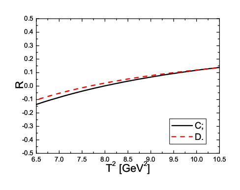
Figure 5: The ratios between the contributions from the negative parity and positive parity doubly heavy baryon states with variations of the Borel parameters T2T^{2}, the AA, BB, CC and DD correspond to the channels Ξc​c\Xi_{cc}, Ωc​c\Omega_{cc}, Ξb​b\Xi_{bb} and Ωb​b\Omega_{bb} respectively.

The fractions

R\displaystyle R =\displaystyle= ∫Δs0d​p0​[ρA​(p0)−ρB​(p0)]​exp⁡[−p02T2]∫Δs0d​p0​[ρA​(p0)+ρB​(p0)]​exp⁡[−p02T2]\displaystyle\frac{\int_{\Delta}^{\sqrt{s_{0}}}dp_{0}\left[\rho^{A}(p_{0})-\rho^{B}(p_{0})\right]\exp\left[-\frac{p_{0}^{2}}{T^{2}}\right]}{\int_{\Delta}^{\sqrt{s_{0}}}dp_{0}\left[\rho^{A}(p_{0})+\rho^{B}(p_{0})\right]\exp\left[-\frac{p_{0}^{2}}{T^{2}}\right]} (13)

are shown explicitly in Fig.5. At the value T2=(2.5−4.0)​GeV2T^{2}=(2.5-4.0)\,\rm{GeV}^{2}, R=(−7∼17)%R=(-7\sim 17)\% in the doubly charmed baryon channels; and at the value T2=(7.5−9.5)​GeV2T^{2}=(7.5-9.5)\,\rm{GeV}^{2}, R=(−4∼10)%R=(-4\sim 10)\% in the doubly bottom baryon channels. The contributions from the negative parity doubly heavy baryon states are not very large, although they are considerable in some sense. In this article, the central values of the threshold parameters are s0=4.2​GeVs_{0}=4.2\,\rm{GeV}, 4.3​GeV4.3\,\rm{GeV}, 10.8​GeV10.8\,\rm{GeV} and 10.9​GeV10.9\,\rm{GeV} in the channels Ξc​c\Xi_{cc}, Ωc​c\Omega_{cc}, Ξb​b\Xi_{bb} and Ωb​b\Omega_{bb} respectively, which are larger than the masses of the corresponding negative parity doubly heavy baryon states, see Table 2. If we take the tensor structures ​p\!\not\!{p} and 11, the contributions from the negative parity baryon states are included in. In the case of the doubly bottom channels, the threshold parameters are slightly larger than the thresholds of the corresponding negative parity baryon states, the contaminations are small, see Fig.5. In fact, without separating the contributions of the positive parity baryon states from the negative parity baryon states explicitly, the two criteria (pole dominance and convergence of the operator product expansion) for choosing the Borel parameter T2T^{2} and threshold parameter s0s_{0} in the conventional QCD sum rules do not work efficiently; we maybe (or maybe not) choose the Borel windows where the contaminations from the negative parity doubly heavy baryon states are large. With suitable Borel parameters, we can choose the tensor structures ​p\!\not\!{p} or 11 to study the masses and pole residues freely. If we choose the tensor structure γ0+1\gamma_{0}+1, the contaminations from the negative parity doubly heavy baryon states are excluded explicitly.

Those doubly heavy baryon states Ξc​c\Xi_{cc}, Ωc​c\Omega_{cc}, Ξb​b\Xi_{bb} and Ωb​b\Omega_{bb} maybe observed at the Tevatron, the LHCb and the PANDA, especially at the LHCb. For example, the Ξc​c\Xi_{cc} and Ωc​c\Omega_{cc} can be produced at the high energy p​ppp or p​p¯p\bar{p} collisions through the gluon-gluon fusion mechanism and the intrinsic charm mechanisms, g+g→(cc)[3S1]3¯+c¯+c¯g+g\to(cc)[^{3}S_{1}]_{\bar{3}}+\bar{c}+\bar{c}, g+g→(cc)[1S0]6+c¯+c¯g+g\to(cc)[^{1}S_{0}]_{6}+\bar{c}+\bar{c}, g+c→(cc)[3S1]3¯+c¯g+c\to(cc)[^{3}S_{1}]_{\bar{3}}+\bar{c}, g+c→(cc)[1S0]6+c¯g+c\to(cc)[^{1}S_{0}]_{6}+\bar{c}, c+c→(cc)[3S1]3¯+gc+c\to(cc)[^{3}S_{1}]_{\bar{3}}+g, c+c→(cc)[1S0]6+gc+c\to(cc)[^{1}S_{0}]_{6}+g, where the (cc)[3S1]3¯(cc)[^{3}S_{1}]_{\bar{3}} (in color anti-triplet 3¯\bar{3}) and (cc)[1S0]6(cc)[^{1}S_{0}]_{6} (in color sextet 𝟔\bf{6}) are two possible SS-wave configurations of the doubly charmed diquark pair (c​c)(cc) inside the baryon states Ξc​c\Xi_{cc} and Ωc​c\Omega_{cc} [37, 38, 39, 40, 41]. The LHCb is a dedicated bb and cc-physics precision experiment at the LHC (large hadron collider). The LHC will be the world’s most copious source of the bb hadrons, and a complete spectrum of the bb hadrons will be available through gluon fusion. Furthermore, once reasonable values of the pole residues λΩ\lambda_{\Omega} and λΞ\lambda_{\Xi} are obtained, we can take them as basic input parameters and study the revelent hadronic processes with the QCD sum rules.

4 Conclusion

In this article, we study the 12+{1\over 2}^{+} doubly heavy baryon states ΩQ​Q\Omega_{QQ} and ΞQ​Q\Xi_{QQ} by subtracting the contributions from the corresponding 12−{1\over 2}^{-} doubly heavy baryon states with the QCD sum rules, and make reasonable predictions for their masses. Those doubly heavy baryon states maybe observed at the Tevatron, the LHCb and the PANDA, especially at the LHCb. Once reasonable values of the pole residues λΩ\lambda_{\Omega} and λΞ\lambda_{\Xi} are obtained, we can take them as basic input parameters and study the revelent hadronic processes with the QCD sum rules.

Acknowledgements

This work is supported by National Natural Science Foundation, Grant Number 10775051, and Program for New Century Excellent Talents in University, Grant Number NCET-07-0282, and the Fundamental Research Funds for the Central Universities.

References

  • [1] M. Mattson et al, Phys. Rev. Lett. 89, 112001 (2002).
  • [2] A. Ocherashvili et al, Phys. Lett. B628, 18 (2005).
  • [3] B. Aubert et al, Phys. Rev. D74, 011103 (2006).
  • [4] R. Chistov et al, Phys. Rev. Lett. 97, 162001 (2006).
  • [5] D. Ebert, R. N. Faustov, V. O. Galkin and A. P. Martynenko, Phys. Rev. D66 (2002) 014008.
  • [6] A. P. Martynenko, Phys. Lett. B663 (2008) 317.
  • [7] W. Roberts and M. Pervin, Int. J. Mod. Phys. A23 (2008) 2817.
  • [8] C. Albertus, E. Hernandez, J. Nieves and J. M. Verde-Velasco, Eur. Phys. J. A32 (2007) 183.
  • [9] J. Vijande, H. Garcilazo, A. Valcarce and F. Fernandez, Phys. Rev. D70, 054022 (2004).
  • [10] S. S. Gershtein, V. V. Kiselev, A. K. Likhoded and A. I. Onishchenko, Phys. Rev. D62, 054021 (2000).
  • [11] A. Valcarce, H. Garcilazo and J. Vijande, Eur. Phys. J. A37 (2008) 217.
  • [12] V. V. Kiselev and A. K. Likhoded, Phys. Usp. 45 (2002) 455.
  • [13] F. Giannuzzi, Phys. Rev. D79 (2009) 094002.
  • [14] D. H. He, K. Qian, Y. B. Ding, X. Q. Li and P. N. Shen, Phys. Rev. D70 (2004) 094004.
  • [15] E. Bagan, M. Chabab and S. Narison, Phys. Lett. B306 (1992) 350.
  • [16] J. R. Zhang and M. Q. Huang, Phys. Rev. D78 (2008) 094007.
  • [17] D. B. Lichtenberg, R. Roncaglia, and E. Predazzi, Phys. Rev. D53, 6678 (1996).
  • [18] M. A. Shifman, A. I. Vainshtein and V. I. Zakharov, Nucl. Phys. B147 (1979) 385, 448.
  • [19] L. J. Reinders, H. Rubinstein and S. Yazaki, Phys. Rept. 127 (1985) 1.
  • [20] S. Narison, Camb. Monogr. Part. Phys. Nucl. Phys. Cosmol. 17 (2002) 1.
  • [21] Z. G. Wang, Phys. Lett. B685 (2010) 59.
  • [22] D. Jido, N. Kodama and M. Oka, Phys. Rev. D54 (1996) 4532.
  • [23] Y. Chung, H. G. Dosch, M. Kremer and D. Schall, Nucl. Phys. B197 (1982) 55.
  • [24] E. Bagan, M. Chabab, H. G. Dosch and S. Narison, Phys. Lett. B301, 243 (1993).
  • [25] Z. G. Wang, Eur. Phys. J. C54 (2008) 231.
  • [26] Z. G. Wang, Eur. Phys. J. C61 (2009) 321.
  • [27] Z. G. Wang, Eur. Phys. J. A44 (2010) 105.
  • [28] Z. G. Wang, arXiv:1001.1652.
  • [29] Z. G. Wang, Phys. Rev. D81 (2010) 036002.
  • [30] B. L. Ioffe, Prog. Part. Nucl. Phys. 56 (2006) 232.
  • [31] P. Colangelo and A. Khodjamirian, hep-ph/0010175.
  • [32] C. Amsler et al, Phys. Lett. B667 (2008) 1.
  • [33] A. Khodjamirian and R. Ruckl, Adv. Ser. Direct. High Energy Phys. 15 (1998) 345.
  • [34] A. A. Ovchinnikov, A. A. Pivovarov and L. R. Surguladze, Int. J. Mod. Phys. A6 (1991) 2025.
  • [35] B. L. Ioffe, Nucl. Phys. B188, 317 (1981).
  • [36] B. L. Ioffe, Z. Phys. C18, 67 (1983).
  • [37] C. H. Chang, C. F. Qiao, J. X. Wang and X. G. Wu, Phys. Rev. D73 (2006) 094022.
  • [38] C. H. Chang, J. P. Ma, C. F. Qiao and X. G. Wu, J. Phys. G34 (2007) 845.
  • [39] C. H. Chang, J. X. Wang and X. G. Wu, Comput. Phys. Commun. 181 (2010) 1144; Comput. Phys. Commun. 177 (2007) 467.
  • [40] S. P. Baranov, Phys. Rev. D54 (1996) 3228.
  • [41] A. V. Berezhnoy, V. V. Kiselev and A. K. Likhoded, Phys. Atom. Nucl. 59 (1996) 870.