A method for tuning parameters of Monte Carlo generators and its application to the determination of the unintegrated gluon density
Abstract
A method for tuning parameters in Monte Carlo generators is described and applied to a specific case. The method works in the following way: each observable is generated several times using different values of the parameters to be tuned. The output is then approximated by some analytic form to describe the dependence of the observables on the parameters. This approximation is used to find the values of the parameter that give the best description of the experimental data. This results in significantly faster fitting compared to an approach in which the generator is called iteratively. As an application, we employ this method to fit the parameters of the unintegrated gluon density used in the Cascade Monte Carlo generator, using inclusive deep inelastic data measured by the H1 Collaboration. We discuss the results of the fit, its limitations, and its strong points.
pacs
24.10.Lx,13.85.HdI Introduction
The substructure of the proton is parametrized in terms of parton distribution functions (PDFs). In perturbative QCD the PDFs are given by solutions of integral equations, for which the initial input distributions have to be determined by global fits to the available experimental data (see, e.g., [1] and references therein). All present global fits are based on fixed-order calculations in , the strong coupling constant, and on factorization theorems that apply to specific inclusive processes, where most of the final-state properties are integrated over.
To study more exclusive processes (i.e., multiparticle production or multidifferential cross sections), Monte Carlo (MC) event generators are used. The physics included in the generators is often not the same as the one described by the factorization theorems and used in global fits. For instance, most of the generators do not implement complete next-to-leading-order (NLO) QCD corrections, but on the other hand they implement parton showers, which partially take into account all-orders resummation effects.
Due to these differences, in principle using in the MC generators the PDFs extracted from global fits is not fully consistent. Ideally, the PDFs should be fitted directly using a MC event generator [2], together with all other extra parameters of the generator. Unfortunately, the parameters of a generator are difficult to tune efficiently because minimization programs require several sequential calls of the generator. This can be extremely time-consuming, especially for more exclusive events.
Motivated by Refs. [3], we are using a fast and efficient method to fit generator parameters. The method is based on using a MC event generator to produce a grid in parameter space for each observable. The parameter dependence is then approximated by polynomials before the fit is performed, which significantly reduces the fitting time. This method has also been recently used in Ref. [4].
As an application, we tune the parameters of the unintegrated gluon distribution function (also called transverse-momentum-dependent gluon distribution function) using the Cascade MC event generator [5], by fitting the generator predictions to inclusive deep inelastic scattering data measured by the H1 Collaboration [6]. We explore the reliability and the limitations of the method and study to which extent the data can constrain the input parameters.
The paper is organized as follows. In section II we give the details of the fitting method. We give a simple example which we generalize to several parameters and observables. In section III, we discuss how the fitting method is applied to a specific case and the results of the tune are presented in section IV. We draw some conclusions at the end of the paper.
II Tuning method
In general, the goal of the tuning is to describe a set of experimental observables , with errors , by means of a theoretical model (in this case a MC generator) that depends on the parameters , and predicts the observables to be , with errors . The values of the parameters that give the best description of the data can be found by minimizing the function
| (1) |
Usually, the minimization is done by numerical programs such as MINUIT [7]. The generator predictions have to be computed typically a few hundred times for different choices of the parameters before the minimum is found. This “brute-force” procedure is highly time consuming.
An alternative approach has been used in, e.g., Ref. [8] as early as twenty years ago, and more recently in Refs. [3, 4]. First, for each observable a grid in parameter space is built, running the MC generator with several values of the parameters. Secondly, the grids are approximated by analytic functions of the parameters, usually polynomials. These functions give a fair description of the generator output and can be used in its stead. In this way, finding the parameter values that best fit the data becomes a much faster task.
The method turns out to be particularly time efficient. A fitting procedure typically requires to sequentially calculate a few hundred times for different values of the parameters. Building the grids in parameter space also requires running the MC generator a few hundred times, but each computation can be done independently in parallel. Once the grid is built and approximated analytically, minimizing the is extremely fast. It becomes very convenient to run the minimization with different initial values of the parameters, or including only a subsample of the observables. However, if new data points are added, a new grid has to be produced for each new data point.
II.1 A simple example
To illustrate the method, we start from a simple example. Suppose we need to fit two data points and with their errors (e.g., two cross-section measurements) using a MC generator with one tunable parameter . In Fig. 1, we indicate the two data points with solid horizontal lines with their error bands.
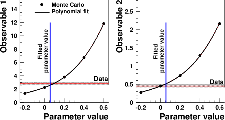
First, we choose 5 values () of the parameter and generate 5 predictions for each observable, i.e., two grids and , with statistical errors due to the Monte Carlo method. In Fig. 1, these grids are indicated by points (the errors are too small to be visible).
Then we choose an analytical form to approximate the two grids, which will be a function of , but also of two new sets of parameters and , one for each grid. To avoid confusion, with denote these new parameters as “grid parameters,” to be distinguished from the original MC parameters. In principle, the functional form itself could be different for each distinct grid, but in practice it is more convenient to choose the same form. To make the procedure easier, it is a good idea to choose a function that is linear in the grid parameters, for instance a third-degree polynomial
| (2) |
The best values of the grid parameters are chosen by means of a minimization for each separate grid. We define this procedure as “grid approximation,” to be distinguished from the actual fit to the experimental data. We define in this case
| (3) |
The polynomials obtained using the best-fit parameter values, are indicated as a curved solid line in Fig. 1. The analysis allows us also to estimate the errors bands on the grid approximations (not visible in the figure).
At this point, it is useful to remark that the degree of the polynomial introduced in Eq. 2 is a matter of choice. Usually, the higher the degree, the better the description of the grids becomes. However, from a certain point on, adding an extra degree does not improve the quality of the approximation significantly, i.e., it does not change significantly the sum of the minimum . In the case shown in Fig. 1, it turns out that a third-degree polynomial gives a much better description of the grid than a second-degree polynomial, while the fourth-degree polynomial does not significantly improve the situation.
Once we have analytical approximations of the Monte Carlo generated grids, we can finally fix the best value of the parameter by minimizing the function
| (4) |
In Fig. 1 the best-fit parameter value, , is indicated as a straight vertical line.
II.2 The general case
Generalizing the above example, with experimental points (denoted by the index ) and parameters (denoted by the index ), we need to build grids in -dimensional spaces, . If we choose points for each parameter, the generation of the grid requires Monte Carlo runs. Once the grids are built, we approximate them using polynomials of degree (for simplicity we show here explicitly only the terms up to second degree)
| (5) |
Note that the Monte Carlo parameters are the variables of the polynomials, while the grid parameters are the coefficients. For degree two and higher, the off-diagonal terms like , , take into account correlations between the Monte Carlo parameters. In our application, we found that third-degree polynomials give a good description of the grid. Advancing to fourth-degree polynomials does not lead to significant improvements.
The total number of coefficients for a degree- polynomial of parameters is . For instance, a polynomial of third degree of four Monte Carlo parameters has 35 coefficients. For simplicity, we denote them collectively as , where , for , for , etc.
The values of the coefficients that give the best approximation to the grid are obtained by minimizing
| (6) |
Since the fit function is linear in the coefficients, the best way to perform the minimization is to use Singular Value Decomposition (SVD) [9]. SVD is based on the fact that the relation between the observables and the grid parameters can be written as an over-determined system of linear equations. SVD provides a solution to this system in a least-squares sense. Compared to other, more general numerical minimization procedures (such as the ones implemented in MINUIT), SVD is faster and guarantees that the true minimum is found. The solution does not depend on the choice of the initial values of the parameters. This is particularly important when the minimization involves several dozens of parameters.
The approximation procedure returns the best-fit values, , of the coefficients and a covariance matrix that can be used to estimate the statistical error bands on the approximation, by means of error propagation.
Once the grids are approximated by polynomials in Monte Carlo parameter space, we finally want to choose the values of the parameters that give the best description of the data. To correctly take into account systematic errors in the experimental measurements, the function has been computed using [10]
| (7) |
where the random parameters are defined in App. A. The minimization is done in this case using MINUIT, since the dependence on parameters is non-linear.
The tuning method studied in Ref. [4] is essentially the same as the one considered here. The main differences between the two implementations reside in the definition of the function, which in our case include the statistical error in the grid approximation () and the contribution of correlated systematic uncertainties.
III An application: fitting the unintegrated gluon distribution function in Cascade
The fitting method described before is general and may be applied to tune any parameter in any Monte Carlo generator. At present, however, we want to concentrate on tuning the parameters of the unintegrated gluon distribution function (uGDF) – also known as transverse-momentum-dependent gluon distribution function – in the Cascade MC generator.
A brief introduction to the Cascade event generator is in order. For a more detailed description we refer the reader to [5]. Cascade is a hadron level Monte Carlo event generator for , and processes, which uses the CCFM evolution equation for the initial state parton shower supplemented with off-shell matrix elements for the hard scattering. To simulate the hadronization process, Cascade uses the Lund string model [11].
The CCFM equation is a linear integral equation which sums up the cascade of gluons under the condition that subsequent emissions are angularly ordered. With this ordering it interpolates between DGLAP (resummation of transverse momenta ) and BFKL (resummation of longitudinal momenta ) limits.
In Fig. 2 we show schematically a parton ladder defining the kinematic variables which we use in equations below.

The CCFM equation reads:
| (8) |
where is the input distribution, denotes the longitudinal momentum fraction of the proton carried by the gluon, is the 2-dimensional transverse momentum of the channel gluon, is the splitting variable, is the factorization scale specified by the maximum allowed angle between the partons in the matrix elements, . We also introduced as a shorthand notation for the 2-dimensional momentum . The Sudakov form factor (which we do not write explicitly) for inclusive quantities regularizes the collinear singularity of the splitting function .
The input distribution can be written as
| (9) |
We choose to parametrize the distribution at the starting scale GeV in the following way
| (10) |
where should be in principle determined from fits. In practice, for the purpose of the present study we fix , GeV, GeV [5]. The value of parameter is dictated by the spectator counting rules[12]: since at large gluons are suppressed as compared to quarks, for gluons has to be larger than 3. Previous studies suggests [13]. Parameter , typically included in global fits of the PDFs (see, e.g., [14, 15]), was set to zero in earlier studies with Cascade [16, 17, 13]. As we will show later, the addition of this parameter substantially improves the description of the data we consider.
The parameters of the starting uGDF, , , and in Eq. 10, are determined by fits to the structure function in inclusive deep inelastic scattering, , as measured by the H1 Collaboration [6]. We chose this data set in order to compare our results with earlier determinations of the uGDF. The measurement was made at the electron-proton center of mass energy GeV within the kinematic range GeV2, . Here is the virtuality of the exchanged boson, and is the Bjorken scaling variable. The measurements cover the small- region where gluon-induced processes dominate and we should have a good sensitivity to the values of the parameters in the uGDF. In total, there are 122 data points binned in and .
We considered two different cases: in the first case we restricted ourselves to and GeV2, as in most of the available Cascade tunes [16, 17, 13]; in the second case, we extended the range to the whole data set.
In summary, we performed four kinds of fits:
The grid in parameter space was built in two different ways depending on whether parameter was set to zero or treated as a fit parameter. The final grids were chosen after performing rough fits with wider grids. In Fit 1 and 3, we chose and for a total of 72 grid points. In Fit 2 and 4, we chose , , and , for a total of 150 grid points. For each point 2.5 million events were generated. Each generation takes a few hours of computing time and can be run in parallel.
Describing the grid with a third degree polynomial is in our experience the best choice. The quality of the grid approximation is very good, with an average of 1.08, 1.05, 1.11, 1.12 for Fit 1 to 4, respectively. We studied the performance of polynomials of different degree. At variance with Ref. [4], we observed that second-degree polynomials do not give a sufficiently good description of the grid. Fourth-degree polynomials perform better but do not lead to a significant improvement of .
Using the covariance matrix obtained in the approximation procedure, the errors of the coefficients in the polynomials are propagated as theoretical errors to the observables we need to fit, denoted as in Eq. (7).
Once the parameter dependence was described by the polynomials, the parameters were fitted to the data by using MINUIT, using the Migrad method [7]. Approximately 150 iterations were needed by the program in order to find the lowest within the allowed limits set by the grid. This minimization took only few seconds.
If our analytical grid description is good enough, we can expect the number of iterations to be the same to if we used the true MC instead of the polynomial approximation. Assuming that running the generator once with the current statistics takes approximately 6 hours of CPU time, fitting the Monte Carlo parameters with a conventional iterative way is expected to take 1506 hours. Clearly, in such case one is forced to drastically reduce the statistics, and the fit could be influenced by statistical fluctuations. In addition, our method allowed us to quickly remake the fit by feeding MINUIT with different starting values. In this way we reduced the risk of finding a local minimum.
IV Results
The best-fit values of the parameters are quoted in Tab. 1.
| Range | (GeV-2) | ||||
|---|---|---|---|---|---|
| Fit 1 | , GeV2 | 0 (fixed) | 2.0 | ||
| Fit 2 | , GeV2 | 1.6 | |||
| Fit 3 | full | 0 (fixed) | 6.2 | ||
| Fit 4 | full | 4.6 |
To have an idea of the performance of our fit, we can compare Fit 1 with earlier uGDF fits [16, 17, 13]. In particular, we chose to compare our fit to the J2003 set 2 (JSET2) uGDF [16], which is the one with the closest conditions to ours. In that set, parameter is set to zero. To compare the quality of the description, we ran Cascade with a statistics of 2.5M events, and we found that our fit gives a , while the old set gives . In other words, we found parameters that give a better description of the data, giving us confidence in our fitting method. In Fig. 3 we show the results of Fit 1, Fit 2, and JSET2 compared to the data. The results of Fit 3 and 4 are shown in Fig. 4.


In order to check if our minimization approach works, we scanned the parameter values around their best values to check if we can indeed identify the signs of the presence of a minimum of . In Fig. 5 and 6 we show how changes as a function of each of the three parameters used in Fit 2 and Fit 4, while fixing the other two to their best-fit value. The scans were carried out using both the Monte Carlo generator directly and the grid approximation. For comparison, we show also the results obtained using second- and fourth-degree polynomial approximations. First of all, we observe that the profile has in all cases a parabolic shape and the position of the minimum is clearly visible. This gives us once again confidence in the reliability of the procedure. We see also that the position of the minimum and the shape of from the MC computation are similar to what is obtained from the grid approximation with third-degree polynomials. The position of the minimum is similar to what is found using the fourth-degree polynomial approximation, but quite different to what is found using the second-degree polynomial approximation. The value of the minimum is not the same for MC and grid approximation (1.4 versus 1.6 for Fit 2; 3.2 versus 4.6 for Fit 4). This is due to the fact that the approximation errors, in Eq. (7), are typically smaller than the MC errors, in Eq. (1), and lead to a higher . This difference becomes irrelevant only if is negligible compared to the experimental errors .


At this point, we can briefly discuss the physical meaning of our results. First of all, we can conclude that in the extended and range of Fit 3 and 4 we cannot achieve a good description of the data with Cascade. This is not surprising, since the generator starts from a purely gluonic distribution function. The description is in general better at lower values of , where gluons dominate.
Secondly, we conclude that in the restricted and range of Fit 1 and 2, a good description of the data is obtained when we include parameter to give more flexibility to the functional form of the gluon distribution.
A few considerations can be made also on the value of parameter , governing the low- behavior of the gluon distribution. In all fits, the value is higher than previous studies [16, 17, 13]. This is for instance the reason of the different behaviors at low and in Fig. 3. The value of turns out to be even higher in the fits with a free parameter.
Not surprisingly, we observe that the parameters of the gluon distribution function are in general different from the ones obtained in global fits at similar input scales [14, 15]. To start with, global fits include many more data sets than we presently considered. However, there are more fundamental differences between the physics included in the generators or in global fits. Therefore, to achieve the best possible description of data with Monte Carlo generators, the parameters of the distribution functions should be tuned independently of global fits.
V Conclusions
In this work we analyzed a method to tune the parameters of Monte Carlo event generators using a set of experimental observables. First, the generator is run with a few different values of the parameters to tune. For each observable, a grid of predictions is thus obtained. The resulting grids are approximated by analytic functions of the parameters. Finally, the analytic functions are used in place of the generator itself to perform a fit to the data and obtain the best values for the parameters. The method is significantly faster than a direct use of the generator, as the construction of the grids typically requires fewer calls to the generator than a direct fit and all grid points can be computed in parallel. There is no need to rerun the generator to repeat the fit with different initial values of the parameters, nor if the experimental data change (for instance if the statistics increase). If data for different observables become available, the generator has to be run to build grids for these new observables, but the old grids remain still valid for the old observables.
The main limit of the approach is that the limited parameter ranges have to be fixed a priori, since the grids have to be built once and for all before the fitting is actually performed. It is possible to improve the choice of the parameter ranges with hindsight, after the first attempt. However, this approach might be time consuming and the minimization can still fail if the data cannot constrain the value of one or more parameters.
As a concrete example, we applied the method to find the best values for the parameters of the unintegrated gluon distribution function used in the Cascade Monte Carlo generator. To constrain the parameter values, we used the data on the structure function in inclusive deep inelastic scattering. We performed four different types of fit, changing the range of and and the number of free parameters under consideration.
Taking the second version of the fit as an illustration, we chose 150 combinations of parameter values and produced a grid of predictions for each one of the 122 data points. The grid was approximated by a third order polynomial with a total of 35 coefficients. The best approximation was searched for using the method of Single Value Decomposition to guarantee a fast and reliable search. The quality of the approximation was found to be very good, with .
Finally, we found the best values of the parameters by a second minimization, using the difference between the experimental measurements and the analytic approximation of the generator output to define the function. The minimization was done using MINUIT.
We checked that the best-fit values of the parameters give a good description of the data, with a . By scanning the dependence of on the single parameters, we strengthened the evidence that the fit found the parameter values that describe the data best.
By including more data in the fit, the method described in this work can be applied to better constrain the parameters of the unintegrated gluon distribution, including those describing the intrinsic -dependence.
Acknowledgements.
Valuable discussions with Hendrik d’Hoeth are thankfully acknowledged. The work of A.B. was partially supported by the SFB “Particles, Strings and the Early Universe” and partially by U.S. DOE Contract No. DE-AC05-06OR23177 under which JSA operates Jefferson Laboratory.Appendix A Treatment of correlated systematic uncertainties
A convenient method to determine the quality of a fit is to use a least square minimization. This ansatz is justified by the assumption that the errors are Gaussian distributed.
A set of measurements {} will in general deviate from a set of corresponding predictions {}. The deviations are caused by various kinds of uncertainties as there is for each data point a statistical uncertainty , an uncorrelated systematic uncertainty and, coming from sources, the correlated systematic uncertainties . The measurement is then related to the prediction by:
| (11) |
where and are added in quadrature to form a unified uncorrelated error . The , express the individual shifts of the data points by the uncertainties and are Gaussian distributed with zero mean and unit variance and assumed to be independent of each other.
A that includes a proper treatment of correlated systematic errors can be calculated as follows (see [10] for a derivation):
| (12) |
where it can be seen that depends both on (the parameters entering the predictions ) and the random parameters . The latter ones can be expressed as
| (13) |
which leads to the -independent form
| (14) |
with
| (15) |
For the systematic errors, in this work we used the ansatz proposed by CTEQ, i.e.,
| (16) |
with being the relative systematic error.
References
- [1] A. Vogt (2007), arXiv:0707.4106 [hep-ph].
- [2] H. Jung (2008), Proceedings of the HERA-LHC workshop, 26-30 May 2008, CERN, CH.
- [3] P. Abreu et al. (DELPHI), Z. Phys. C73, 11 (1996).
- [4] A. Buckley, H. Hoeth, H. Lacker, H. Schulz, and J. E. von Seggern (2009), arXiv:0907.2973 [hep-ph].
- [5] H. Jung, Comput. Phys. Commun. 143, 100 (2002).
- [6] C. Adloff et al. (H1), Eur. Phys. J. C21, 33 (2001).
- [7] F. James and M. Roos, Comput. Phys. Commun. 10, 343 (1975).
- [8] W. Braunschweig et al. (TASSO), Z. Phys. C41, 359 (1988).
- [9] W. H. Press, S. A. Teukolsky, W. T. Vetterling, and B. P. Flannery, Numerical recipes in FORTRAN: the art of scientific computing (Cambridge University Press, New York, NY, USA, 1992).
- [10] D. Stump et al., Phys. Rev. D65, 014012 (2001).
- [11] B. Andersson, G. Gustafson, G. Ingelman, and T. Sjostrand, Phys. Rept. 97, 31 (1983).
- [12] S. J. Brodsky and G. R. Farrar, Phys. Rev. Lett. 31, 1153 (1973).
- [13] H. Jung, A. V. Kotikov, A. V. Lipatov, and N. P. Zotov (2006), arXiv:hep-ph/0611093.
- [14] M. Gluck, P. Jimenez-Delgado, and E. Reya, Eur. Phys. J. C53, 355 (2008).
- [15] A. D. Martin, W. J. Stirling, R. S. Thorne, and G. Watt (2009), arXiv:0901.0002 [hep-ph].
- [16] M. Hansson and H. Jung (2003), arXiv:hep-ph/0309009.
- [17] H. Jung (2004), arXiv:hep-ph/0411287.