Percolation on self-dual polygon configurations

In 1963 Sykes and Essam [30] noticed that, in independent bond percolation, a star with bond probabilities $p_{1}$, $p_{2}$ and $p_{3}$ may be replaced by a triangle with bond probabilities $r_{1}$, $r_{2}$ and $r_{3}$, provided the $p_{i}$ and $r_{i}$ satisfy certain equations; in particular, a star in which each bond has probability $p_{0}=1-2\sin(\pi/18)$ of being open may be replaced by a triangle with bond probabilities $1-p_{0}$. Sykes and Essam went on to use this star-triangle transformation to predict that $p_{0}$ and $1-p_{0}$ should be the critical probabilities for bond percolation on the hexagonal and triangular lattices, respectively. In 1981 Wierman [31] gave a rigorous proof of this result with the aid of a Russo–Seymour–Welsh-type theorem. In 1982 Kesten [17] extended Wierman’s theorem to describe the ‘critical surface’ of weighted bond percolation on the triangular lattice, although the details were worked out only in 1999 by Grimmett [13]. Later, in 2008, it was shown [7] that the sum of the critical probabilities of a centrally symmetric planar lattice and its dual is 1; more generally, an analogous statement allowing for percolation with different probabilities for different bonds was proved, giving the Kesten–Grimmett theorem as an easy corollary.

In 1984 Wierman [32] used the general star-triangle transformation to determine the exact critical probability for bond percolation (with equal bond probabilities) on a lattice obtained from the square lattice by adding some diagonals. Using a simpler transformation, Suding and Ziff [29] deduced the critical probability for site percolation on the extended Kagomé lattice from Wierman’s result for the hexagonal lattice.

Recently, extending work of Scullard [24] and Chayes and Lei [10], Ziff [35] and Ziff and Scullard [36] proposed a simple criterion predicting the value of the critical probability for a wide variety of percolation models in the plane. In addition to the usual independent site and/or bond percolation models on a number of lattices, these models include cases which can be seen as bond percolation with local dependencies between the states of certain bonds.

The predictions of Scullard and Ziff are similar in nature to those of Sykes and Essam [30] mentioned above: having shown that for a certain probability $p_{0}$ the percolation model is ‘self-dual’, they state that this probability $p_{0}$ is therefore critical. Mathematically, there is a folklore ‘conjecture’ (with, as far as we are aware, no precise formulation) stating that any ‘reasonable’ self-dual planar model is critical. This conjecture is still wide open. It is well known to hold in certain special cases, in particular for site or bond percolation on lattices with certain symmetries, such as reflection in a line (see Kesten [17]), or rotational symmetry of any order, as shown in [7]. More generally, as remarked in [7], it can be shown for site or bond percolation on any lattice by combining results of Sheffield [27, Corollary 9.4.6], Aizenman, Kesten and Newman [1] and Menshikov [21].

Chayes and Lei [10] independently described a special case of the Scullard–Ziff criterion (as well as a generalization to random cluster models), and gave a sketch proof of criticality under an extra assumption. In a recent preprint, Wierman and Ziff [33] proved criticality in certain special cases, using known results on self-dual planar lattices.

In this paper we shall prove that the Scullard–Ziff criterion does indeed give the critical point for a wide variety of planar percolation models. In the original papers in the physics literature, the exact scope of applicability of the criterion is not entirely clear. In this paper we shall define precisely a general class of models that are self-dual in the appropriate sense, and use new methods to show that the self-dual point is indeed critical in all cases.

Although full definitions will be given only in the next section, let us illustrate some simple special cases of our main result, starting with one very concrete (but rather specific) example, and then turning to a more general family.

Even the very special cases described above are outside the scope of existing results, for several reasons. Firstly, in general they do not correspond to independent bond or site percolation on any lattice (as required in [33]). This is certainly the case when increasing events are not positively correlated; see the discussion in Section 2. Such correlation is absent in Example 1.1 when $p$ is equal to or close to $1/2$, since $p^{3}<(p(1-p)+p^{3})^{2}$ when $p=1/2$. Positive correlation is also required for the arguments in [10]. Secondly, in Example 1.2 there is no rotational or reflectional symmetry, as required in [33] and in [10], so existing Russo–Seymour–Welsh-type results do not apply.

Our results show that self-duality implies criticality in a context that is much broader than the Scullard–Ziff criterion; an example is given in Figure 2.7.

Mathematically, the main interest of this paper is perhaps in the development of new tools needed to analyze the general model, including new proofs of analogues of the Russo–Seymour–Welsh Lemma, and a generalization of Harris’s Lemma. The rest of the paper is organized as follows. In Section 2 we describe the model we shall study, and state our main results. In Section 3 we present a generalization of Harris’s Lemma to products of posets. In Section 4 we prove various technical results about the model. The heart of the paper is Section 5, where we prove a new RSW-type lemma; the proof is rather involved, so we first illustrate the ideas in a simpler setting (bond percolation on ${\mathbb{Z}}^{2}$) in Subsection 5.1. In Section 6 we show how to apply this lemma using only the minimal symmetry guaranteed by self-duality. Finally, in Section 7 we show that (as in [4]), using a suitable sharp-threshold result, it is but a small step from rectangle crossings to the final results. In Section 8 we conclude with a brief discussion of the behaviour of the model in the critical case.

The starting point of our investigation is an embedding of a suitable hypergraph in the plane, as described implicitly by Ziff and Scullard [36] and explicitly by Wierman and Ziff [33]. In these papers the hypergraphs considered are 3-uniform, but much of the time there is no need for this restriction. Since the concept of a plane hypergraph seems fundamental, we give several equivalent definitions. To avoid irrelevant difficulties we always assume piecewise linearity of all curves.

By a polygon we mean a piecewise-linear closed curve $P$ in the plane that, if it touches itself at all, does so only externally at some vertices. (To be pedantic, $P$ is the image of some regular $n$-gon $P^{\prime}$ under a piecewise linear map defined on the closed domain bounded by $P^{\prime}$ that is injective except possibly at the vertices of $P^{\prime}$.) Such a polygon surrounds (more precisely winds around) a simply connected open set that we call its interior.

By a plane hypergraph ${\mathcal{H}}$ we mean a set of points of ${\mathbb{R}}^{2}$, the vertices, together with a set of polygons, the hyperedges, with the following properties:

1. (i)

   any bounded subset of the plane contains only finitely many vertices, and meets only finitely many hyperedges,

2. (ii)

   the interiors of the hyperedges are disjoint,

3. (iii)

   each hyperedge is incident with at least one vertex, and

4. (iv)

   hyperedges meet themselves or each other only at vertices.

Note that we allow a hyperedge to meet the same vertex several times, as in Figure 2.1, simply because there turns out to be no reason not to. Property (i) ensures that each vertex meets only finitely many hyperedges, and vice versa. In this paper, all plane hypergraphs we consider are connected, in the natural sense.

Two plane hypergraphs are isomorphic if there is a homeomorphism from the plane to itself mapping one into the other, in the obvious sense. Of course, given a plane hypergraph (or indeed an isomorphism class of plane hypergraphs) there is a corresponding abstract hypergraph; more precisely, a (multi-)hyper(-multi-)graph, where we have included ‘multi’ twice to indicate that two or more hyperedges may be incident with the same set of vertices, and a single hyperedge may be incident with a vertex more than once. However, we shall work directly with the drawings throughout.

Plane hypergraphs are natural generalizations of plane (multi)graphs. Indeed, we may think of a plane graph as a representation of an abstract graph, with the vertices represented by points, and the edges by connected sets meeting only at the vertices. The edges of a graph are naturally represented by minimal sets connecting the corresponding vertices, i.e., simple curves, but in the hypergraph case polygons are more natural, so we use them even for hyperedges with only two vertices (or indeed, one vertex). When we come to percolation in a moment, the idea is that instead of each edge in a graph randomly either connecting its vertices or not, independently of the other edges, each hyperedge will randomly connect some subsets of its vertices, independently of the other hyperedges.

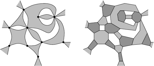
It is easy to check that (connected, as always in this paper) plane hypergraphs ${\mathcal{H}}$ correspond exactly to shaded locally finite connected plane multigraphs $G$, where the faces of $G$ are properly coloured grey and white, so that every edge borders faces of different colours, with any unbounded faces white. (At this stage there may be one or more unbounded faces; in the bulk of the paper all faces will be bounded.) Indeed, vertices correspond to vertices, and the hyperedges of ${\mathcal{H}}$ are simply the grey faces of $G$, as on the left in Figure 2.1. Of course, a plane graph $G$ with at most one unbounded face has an appropriate shading if and only if every degree is even, and then it has either one or two shadings, depending on whether or not it has an unbounded face.

Note that if $e$ is a hyperedge incident with $|e|$ vertices (counting multiplicity), then, as a polygon, $e$ is made up of $|e|$ segments joining vertices, corresponding to the edges of $G$. We cannot in general draw these segments as straight lines. For example, ${\mathcal{H}}$ may contain triples $uvw$ and $uvw^{\prime}$, say; furthermore, there may be further hyperedges inside the region bounded by the two curves joining $u$ and $v$ associated to these triples.

By a face of a plane hypergraph ${\mathcal{H}}$ (defined as above) we mean a component of what is left of the plane after removing all hyperedges and their interiors, i.e., a white face of the corresponding graph $G$. For our next few definitions (in particular that of duality) to make sense, it is convenient to insist that each face of ${\mathcal{H}}$ has finitely many edges in its boundary. This is equivalent to imposing the condition that if ${\mathcal{H}}$ is infinite, then it has no unbounded faces. (Of course, if ${\mathcal{H}}$ is finite, then it necessarily has exactly one unbounded face.) When it comes to percolation, we naturally consider only infinite ${\mathcal{H}}$.

There is yet another way of defining plane hypergraphs, which will turn out to be much more convenient to work with, but is at first sight perhaps less natural (at least for percolation). Given a (connected, as usual) plane hypergraph ${\mathcal{H}}$ and the corresponding graph $G$ as above, replace each vertex $v$ of ${\mathcal{H}}$ by a black $2d$-gon, where $d=d(v)$ is the degree of $v$, each face by a white $2d$-gon, where $d$ is the number of edges (of $G$) bounding the face, and each hyperedge $e$ incident with $d$ vertices (counted with multiplicity) by a grey $2d$-gon. In this way we obtain a cubic planar map $M$ in which the faces are properly coloured black, white and grey; see Figure 2.1. (As before, we cannot necessarily draw the edges of the polygons as straight lines.)

The reverse transformation is even simpler: starting from a cubic map $M$ (i.e., a connected locally finite 3-regular plane graph in which each face has finitely many edges in its boundary) in which the faces are properly coloured black, white and grey, we simply contract each black face to a point to form a vertex of ${\mathcal{H}}$, and take the grey faces to form the hyperedges. In what follows we shall refer to such a coloured map $M$ as a map hypergraph (or simply a hypergraph, when there is no danger of confusion), and denote it also by ${\mathcal{H}}$.

Note that when ${\mathcal{H}}$ is a graph (i.e., ${\mathcal{H}}$ is 2-uniform), then the corresponding map is the one considered in Chapter 3 of [6] (see Figures 2 and 4, for example). There, the 4-gon corresponding to an edge is coloured black or white according to whether the edge is open or closed; here, the $2|e|$-gon corresponding to a hyperedge $e$ is grey for now, but will be coloured with a mixture of black and white later.

By a plane hyperlattice ${\mathcal{H}}$ we shall mean an infinite connected plane hypergraph (defined in any of the three ways above) with a lattice ${\mathcal{L}}$ of translational symmetries, i.e., such that there are linearly independent vectors ${\bf a}$ and ${\bf b}$ with the property that translation of the plane through either vector maps the drawing into itself in the obvious sense, corresponding to an isomorphism of the underlying hypergraph. Throughout, we view ${\mathcal{L}}=\{m{\bf a}+n{\bf b}:m,n\in{\mathbb{Z}}\}$ as a subset of ${\mathbb{R}}^{2}$. More formally, we define a plane hyperlattice to be a pair $({\mathcal{H}},{\mathcal{L}})$ as above, since in what follows ${\mathcal{L}}$ need not be the full lattice of translational symmetries of ${\mathcal{H}}$; in spite of this, we usually omit ${\mathcal{L}}$ from the notation. Naturally, when we consider isomorphisms of plane hyperlattices, these are required to preserve the corresponding lattices of symmetries. More precisely, a homeomorphism $S:{\mathbb{R}}^{2}\to{\mathbb{R}}^{2}$ is an isomorphism from the plane hyperlattice $({\mathcal{H}},{\mathcal{L}})$ to $({\mathcal{H}}^{\prime},{\mathcal{L}}^{\prime})$ if it corresponds to a plane hypergraph isomorphism and satisfies $S(x+\ell)=S(x)+T(\ell)$ for all $x\in{\mathbb{R}}^{2}$ and $\ell\in{\mathcal{L}}$, where $T$ is a linear map with $T({\mathcal{L}})={\mathcal{L}}^{\prime}$.

In the context of percolation, the natural notion of the dual of a plane hypergraph ${\mathcal{H}}$ turns out to be the plane hypergraph ${\mathcal{H}}^{*}$ defined as follows. Take a vertex of ${\mathcal{H}}^{*}$ inside each face of ${\mathcal{H}}$. To obtain the hyperedges of ${\mathcal{H}}^{*}$, replace each hyperedge $e$ of ${\mathcal{H}}$ by the dual hyperedge $e^{*}$ joining the vertices corresponding to the faces that $e$ meets, as in Figure 2.2.

In the special case of 2-uniform hypergraphs, i.e., graphs, this is the usual notion of planar duality. In the 3-uniform case considered (with mild additional restrictions) by Wierman and Ziff [33], the notion of duality just defined coincides with theirs; the description of Ziff and Scullard [36] seems to be ambiguous.

In terms of the shaded graph $G$, the operation of taking the dual is rather complicated – it is not simply reversing the shading. However, in the 3-coloured map formulation, it is very simple to construct the dual: simply exchange black and white. Indeed, one can think of a hyperedge and its dual together as corresponding to a grey face of the map $M$ (for example, in Figure 2.2 one can take the intersection of $e$ and $e^{*}$ as the grey face); the vertices of ${\mathcal{H}}$ correspond to the black faces of $M$, and the vertices of ${\mathcal{H}}^{*}$ to the white faces of $M$.

Of course, choosing the drawing appropriately, we may take the dual ${\mathcal{H}}^{*}$ of a plane hyperlattice ${\mathcal{H}}$ to be a plane hyperlattice, and the dual of ${\mathcal{H}}^{*}$ to be ${\mathcal{H}}$. A plane hyperlattice ${\mathcal{H}}$ is self-dual if ${\mathcal{H}}^{*}$ is isomorphic to ${\mathcal{H}}$; examples are shown in Figures 2.2, 2.5 and 2.7.

If $P$ is a polygon in the plane, then by a non-crossing partition of its vertex set $V(P)$ we mean a partition $\pi$ such that no two distinct parts of $\pi$ contain interlaced pairs of vertices: if $x$, $y$, $z$, $w$ are four distinct vertices appearing in this cyclic order around $P$, a non-crossing partition $\pi$ cannot contain two parts one of which includes $x$ and $z$, and the other $y$ and $w$. Equivalently, a partition $\pi$ of $V(P)$ is a non-crossing partition if and only if it may be realized by constructing disjoint (path-)connected subsets $S_{i}$ of $P$ (which we take to include its interior) so that each part of $\pi$ is the intersection of some $S_{i}$ with $V(P)$.

The dual $\pi^{*}$ of a non-crossing partition $\pi$ is the non-crossing partition of the edges of $P$ in which two edges $e$ and $f$ are in the same part if and only if they are not interlaced with two vertices $x$ and $y$ in a common part of $\pi$. Here interlaced means that the edges and vertices occur in the cyclic order $e$, $x$, $f$, $y$ or its reverse.

Turning finally to percolation, the state of a hyperedge $e$ will simply be a non-crossing partition of its vertices. (More precisely, of the incidences of $e$ with its vertex set, so if $e$ touches itself, the relevant vertex appears multiple times in the groundset of the partition.) A configuration $\omega$ is an assignment of a state to each hyperedge of the hypergraph ${\mathcal{H}}$ under consideration. We think of the state of a hyperedge $e$ as describing connections within $e$. In particular, by an open path in a configuration $\omega$ we mean a sequence $v_{0}e_{1}v_{1}e_{2}\ldots e_{\ell}v_{\ell}$ such that, for each $i$, the partition of the vertices of $e_{i}$ has a part containing both $v_{i-1}$ and $v_{i}$. Two vertices are connected in $\omega$ if they are joined by an open path, and the open clusters of $\omega$ are the maximal connected sets of vertices.

Finally, a hyperlattice percolation model consists of a plane hyperlattice $({\mathcal{H}},{\mathcal{L}})$ together with a probability measure on configurations on ${\mathcal{H}}$ such that the states of different hyperedges are independent, and the measure is preserved by the action of ${\mathcal{L}}$. In other words, if $e^{\prime}$ is a translate of $e$ under an element of ${\mathcal{L}}$, then corresponding states in $e^{\prime}$ and $e$ have the same probabilities. Note that for a single hyperedge $e$, all probability distributions on the set of non-crossing partitions associated to $e$ are allowed.

As usual, the sigma-field of measurable events is the one generated by cylindrical sets, i.e., by events depending only on the states of a finite set of hyperedges. In fact, except when defining percolation, throughout this paper we can work with large enough finite regions of ${\mathcal{H}}$, so there are no issues of measurability.

The dual $\omega^{*}$ of a configuration $\omega$ on ${\mathcal{H}}$ is the configuration on ${\mathcal{H}}^{*}$ in which the state of $e^{*}$ is the dual of the state of $e$ (noting that vertices of $e^{*}$ correspond to edges of the polygon $e$). It is not hard to check that finite open clusters in $\omega$ are surrounded by open cycles in $\omega^{*}$ and vice versa; this is most easily seen in the colouring formulation described at the start of Section 4.

Given a plane hyperlattice $({\mathcal{H}},{\mathcal{L}})$, suppressing ${\mathcal{L}}$ in the notation as usual, the hyperlattice percolation models on ${\mathcal{H}}$ may be parametrized as follows. First pick one representative $e_{i}$ of each orbit of the action of ${\mathcal{L}}$ on the hyperedges. Then for each non-crossing partition $\pi$ of the vertices of $e_{i}$, choose a probability $p_{i,\pi}$, subject only to $\sum_{\pi}p_{i,\pi}=1$ for each $i$. We call such a vector ${\bf p}=(p_{i,\pi})_{i,\pi}$ a probability vector (for ${\mathcal{H}}$), and write ${\mathcal{H}}({\bf p})$ for the corresponding percolation model. The dual vector ${\bf p}^{*}$ assigns the probability $p_{i,\pi}$ to the partition $\pi^{*}$ of $e_{i}^{*}$, so ${\mathcal{H}}^{*}({\bf p}^{*})$ is a hyperlattice percolation model on ${\mathcal{H}}^{*}$.

The hyperlattice percolation model ${\mathcal{H}}({\bf p})$ is self-dual if ${\mathcal{H}}({\bf p})$ and ${\mathcal{H}}^{*}({\bf p}^{*})$ are isomorphic, i.e., if there is an isomorphism from ${\mathcal{H}}$ to ${\mathcal{H}}^{*}$ such if $e\in E({\mathcal{H}})$ and $f\in E({\mathcal{H}}^{*})$ correspond under the isomorphism, then each partition $\pi$ of $f$ has the same probability in ${\mathcal{H}}^{*}({\bf p}^{*})$ as the corresponding partition of $e$ does in ${\mathcal{H}}({\bf p})$. Our aim is to show that self-dual hyperlattice models are ‘critical’, but first we must define what critical means.

The set of partitions of a (here finite) set $S$ forms a poset ${\mathcal{P}}$ in a natural way: we have $\pi\preccurlyeq\pi^{\prime}$ if any two elements in the same part of $\pi$ are in the same part of $\pi^{\prime}$, i.e., the parts of $\pi^{\prime}$ are unions of those of $\pi$, i.e., if $\pi$ refines $\pi^{\prime}$.

Given a hyperedge $e_{i}$ as above, let ${\mathcal{P}}={\mathcal{P}}_{e_{i}}$ be the poset formed by the non-crossing partitions of the vertices of $e_{i}$. An upset ${\mathcal{U}}$ in ${\mathcal{P}}$ is a subset of ${\mathcal{P}}$ such that if $\pi\in{\mathcal{U}}$ and $\pi\prec\pi^{\prime}$ then $\pi^{\prime}\in{\mathcal{U}}$. Given an upset ${\mathcal{U}}$ in ${\mathcal{P}}_{e_{i}}$ and a probability vector ${\bf p}$, let $p_{i}({\mathcal{U}})=\sum_{\pi\in{\mathcal{U}}}p_{i,\pi}$ denote the probability that the state of $e_{i}$ is in ${\mathcal{U}}$. Given two probability vectors ${\bf p}$ and ${\bf q}$, we say that ${\bf q}$ dominates ${\bf p}$ if $q_{i}({\mathcal{U}})\geq p_{i}({\mathcal{U}})$ for each $i$ and each upset ${\mathcal{U}}\subset{\mathcal{P}}_{e_{i}}$. We say that ${\bf q}$ strictly dominates ${\bf p}$, and write ${\bf q}\succ{\bf p}$, if $q_{i}({\mathcal{U}})>p_{i}({\mathcal{U}})$ for each $i$ and each non-trivial upset ${\mathcal{U}}\subset{\mathcal{P}}_{e_{i}}$, i.e., for all upsets apart from ${\mathcal{U}}=\emptyset$ and ${\mathcal{U}}={\mathcal{P}}_{e_{i}}$. Note that we can have ${\bf p}\neq{\bf q}$ such that ${\bf q}$ dominates ${\bf p}$ but does not strictly dominate it.

Hall’s theorem implies that ${\bf q}$ dominates ${\bf p}$ if and only if ${\bf q}$ can be obtained from ${\bf p}$ by moving ‘probability mass’ from elements $p_{i,\pi}$ to elements $p_{i,\pi^{\prime}}$ with $\pi\prec\pi^{\prime}$. In the case of strict domination, we can assume that, for each $i$, a non-zero mass is moved from each $\pi$ to each $\pi^{\prime}\succ\pi$.

A percolation model ${\mathcal{H}}({\bf p})$ percolates if the probability that the open cluster containing any given vertex is infinite is positive. As usual, this is equivalent to the existence with probability 1 of an infinite open cluster. The model ${\mathcal{H}}({\bf p})$ is critical if two conditions hold: for any ${\bf q}\succ{\bf p}$ the model ${\mathcal{H}}({\bf q})$ percolates, and for any ${\bf q}\prec{\bf p}$ the model ${\mathcal{H}}({\bf q})$ does not percolate.

We say that the model ${\mathcal{H}}({\bf p})$ exhibits exponential decay (of the volume) if there is a constant $\alpha>0$ such that for any fixed vertex $v$ the probability that the open cluster containing $v$ contains at least $n$ vertices is at most $e^{-\alpha n}$ for all $n\geq 2$. Our main result is the following.

Although this is far from the main point, a very special case is that the critical probability for bond percolation on any self-dual planar lattice is $1/2$. Note that the condition ${\bf q}\succ{\bf p}$ is stronger than what one could hope for, namely a similar result with this condition replaced by ${\bf q}$ dominating ${\bf p}$ and ${\bf q}\neq{\bf p}$. However, one would then need to rule out degenerate special cases (corresponding to increasing the probability of bonds that are ‘dead ends’ in a bond percolation model, for example). Also, Theorem 2.1 with the present conditions is strong enough for the main application, Corollary 2.3 below.

It turns out that in proving Theorem 2.1, we do not require an exact isomorphism between ${\mathcal{H}}({\bf p})$ and ${\mathcal{H}}^{*}({\bf p}^{*})$. We call two hyperlattice percolation models ${\mathcal{H}}_{1}({\bf p}_{1})$ and ${\mathcal{H}}_{2}({\bf p}_{2})$ equivalent if they can be coupled so that, for some constant $C$, for every open path $P$ in either model there is an open path $P^{\prime}$ in the other model at Hausdorff distance at most $C$ from $P$. Roughly speaking, the typical reason for two models to be equivalent is that they can be viewed as different ways of realizing a single underlying model.

For example, consider a plane triangulation $G$ with a lattice ${\mathcal{L}}$ of translational symmetries, such as the triangular lattice. Then there are two natural ways to form a hyperlattice from $G$, illustrated (for a more complicated lattice) in Figure 2.3.

In the first, there is a vertex for each edge of $G$, in the second, a vertex for each face of $G$. In either case, there is a hyperedge for each vertex $v$ of $G$; this hyperedge is incident to all vertices corresponding to edges or faces of $G$ that $v$ is incident to. Within each hyperedge, assign probability $p$ to the partition in which all vertices are in a single part, and $1-p$ to that in which every vertex is in a separate part. Let us call a hyperedge open if we select the partition into one part, and closed otherwise. Then the resulting models ${\mathcal{H}}(p)$ and ${\mathcal{H}}^{\prime}(p)$ are equivalent using the natural coupling, i.e., the coupling in which the hyperedges in the two models corresponding to a vertex $v$ of $G$ have the same state, open or closed. Indeed, in either model an open path of length more than 1 consists of a sequence of open hyperedges with consecutive ones sharing (hyperlattice) vertices. But two hyperedges share a vertex in ${\mathcal{H}}$ if and only if the corresponding vertices of $G$ are joined by an edge, and share a vertex in ${\mathcal{H}}^{\prime}$ if and only if the corresponding vertices of $G$ are in a common face. In a triangulation, two vertices are in a common face if and only if they are joined by an edge.

Emphasizing the lattice in the notation, for a change, we say that a hyperlattice percolation model $({\mathcal{H}}({\bf p}),{\mathcal{L}})$ is approximately self-dual if there is a model $({\mathcal{H}}^{\prime}({\bf p}^{\prime}),{\mathcal{L}})$ equivalent to $({\mathcal{H}}^{*}({\bf p}^{*}),{\mathcal{L}})$ such that $({\mathcal{H}}^{\prime}({\bf p}^{\prime}),{\mathcal{L}})$ and $({\mathcal{H}}({\bf p}),{\mathcal{L}})$ are isomorphic as plane hyperlattices, with the corresponding linear map $T$ an isometry of the plane. The last restriction is a technicality: in the case of (exact) self-duality we did not impose it, but as we shall see in Lemma 6.7, any isomorphism witnessing self-duality has this property (after a suitable affine transformation). This is presumably also true for approximate self-duality, but as the condition will (we believe) self-evidently hold in any applications, we do not bother checking this. For our proofs, approximate self-duality is (apart from one technicality) just as good as self-duality, so we obtain the following strengthening of Theorem 2.1. In this result ‘malleability’ is a technical condition we shall introduce later (see Definitions 5.8 and 5.9); in the 3-uniform case, all hyperlattice percolation models are malleable. Also, any ‘site percolation’ model, where only the partition into singletons and that into a single part occur, is malleable.

To indicate that this extension may be useful, consider a plane triangulation $G$ with a lattice of translational symmetries, and a real number $0<p<1$. Consider the two hyperlattice percolation models ${\mathcal{H}}(p)$ and ${\mathcal{H}}^{\prime}(p)$ corresponding to site percolation on $G$, defined as above. Then ${\mathcal{H}}$ and ${\mathcal{H}}^{\prime}$ are dual to each other, so ${\mathcal{H}}(p)$ and ${\mathcal{H}}^{\prime}(1-p)$ are dual as hyperlattice percolation models. Since, as noted above, ${\mathcal{H}}(p)$ and ${\mathcal{H}}^{\prime}(p)$ are equivalent, we see that ${\mathcal{H}}(1/2)$ is approximately self-dual, so Theorem 2.2 implies that the critical probability for site percolation on $G$ is $1/2$. In itself this is not new (see the discussion in the introduction), but it indicates that the models to which Theorem 2.2 applies include ones with a site percolation ‘flavour’.

We have just seen that site percolation on a triangulation with a lattice of symmetries, which for $p=1/2$ is easily seen to be self-dual in an appropriate sense, may be transformed to a hyperlattice percolation model that is only approximately self-dual. In this case, the duality is clearer in the site percolation formulation than the hyperlattice one. Unsurprisingly, there are also cases where the reverse holds. Indeed, for any plane hyperlattice ${\mathcal{H}}$, selecting only the partitions in which all vertices in a given edge are connected or none are, we obtain a site percolation model on an (in general non-planar) graph. For example, taking ${\mathcal{H}}$ as in Figure 1.2, one obtains the non-planar graph in Figure 2.4.

Theorem 2.1 shows that if ${\mathcal{H}}$ is self-dual, then the critical probability for site percolation on the resulting graph is $1/2$.

Returning to the original motivation, the key observation of Ziff [35] and Ziff and Scullard [36] (present also in the original papers of Scullard [24] and Chayes and Lei [10] in the special case where ${\mathcal{H}}$ is the ‘triangular hyperlattice’ $T$ shown in Figure 2.5) is that if ${\mathcal{H}}$ is 3-uniform, then the condition for self-duality becomes very simple, at least if one takes the same connection probabilities in all triangles. Unfortunately, this involves some further definitions, to allow for non-symmetric cases.

By a labelled plane hyperlattice we mean a plane hyperlattice in which the vertices around each hyperedge are labelled $1,2,\ldots,k$ in a way that is consistent with either the clockwise or anti-clockwise cyclic order within each hyperedge, and is globally consistent with the lattice ${\mathcal{L}}$ of translational symmetries. When $k=3$ or $k=4$ we often use letters $A$, $B,\ldots,$ to denote the labels rather than numbers. In the 3-uniform case, assigning labels as above amounts to designating the vertices of a hyperedge $e$ as its $A$-, $B$- and $C$-vertex in any order, as in [33]. The simplest example of a labelled plane hyperlattice is the labelled triangular hyperlattice shown in Figure 2.5. Another example is illustrated in Figure 2.6.

Note that the $A$-vertex of one hyperedge may be the $B$-vertex of another hyperedge (or indeed, of the same hyperedge if it touches itself). Given a $k$-uniform labelled plane hyperlattice and a probability vector ${\bf p}$ consisting of probabilities $p_{\pi}$, $\pi\in{\mathcal{P}}_{\{1,2,\ldots,k\}}$, that sum to $1$, there is a corresponding hyperlattice percolation model ${\mathcal{H}}({\bf p})$: for every hyperedge $e$, we assign $p_{\pi}$ as the probability that the vertices of $e$ are partitioned according to $\pi$, with the groundset $\{1,2,\ldots,k\}$ of $\pi$ corresponding to the vertices of $e$ in a manner indicated by the labelling.

Specializing to the 3-uniform case, the dual $e^{*}$ of an edge $e$ inherits a labelling from $e$: take the first vertex to be the one opposite the first vertex of $e$, and so on, so a labelled 3-uniform plane hyperlattice ${\mathcal{H}}$ has a dual ${\mathcal{H}}^{*}$ that is again a labelled 3-uniform plane hyperlattice.

If $AcBaCb$ is a triangle with vertices $A$, $B$, $C$ and edges $a$, $b$ and $c$, then there are five possible partitions of the vertex set, all of which are non-crossing. These are represented by Wierman and Ziff [33] as $A|B|C$, $AB|C$, $AC|B$, $BC|A$, and $ABC$; we use the more compact notation $\emptyset$, $AB$, $AC$, $BC$ and $ABC$. The duals of these partitions are, respectively, $abc$, $ab$, $ac$, $bc$ and $\emptyset$. In this setting, a probability vector ${\bf p}$ is simply a vector ${\bf p}=(p_{\emptyset},p_{AB},p_{AC},p_{BC},p_{ABC})$ of non-negative reals summing to $1$, and the dual of ${\mathcal{H}}({\bf p})$ is simply ${\mathcal{H}}^{*}({\bf p}^{*})$, where ${\bf p}^{*}$ is formed from ${\bf p}$ by interchanging $p_{\emptyset}$ and $p_{ABC}$.

The observation of Scullard and Ziff mentioned earlier may be formulated as follows: if the labelled plane hyperlattice ${\mathcal{H}}$ is self-dual, then the model ${\mathcal{H}}({\bf p})$ is self-dual if and only if $p_{\emptyset}=p_{ABC}$. The key point is that the other three partitions are all self-dual, as long as the dual triangle is labelled in the appropriate way, so only two entries in the probability vector, namely $p_{\emptyset}$ and $p_{ABC}$, change when we pass to the dual. [In the papers [35, 36], the formulation of duality is not totally clear. Wierman and Ziff [33] clearly formulate the notion of self-duality for unlabelled plane hyperlattices, and state that one can consider any labelling with lattice structure, but this seems to be an oversight; one needs the labelled hyperlattice to be self-dual as a labelled hyperlattice, which is not always the case.]

If the probabilities in ${\bf p}$ are appropriate functions of a single parameter $p$, the condition $p_{\emptyset}=p_{ABC}$ allows one to determine the critical point of the model; in general it gives the critical surface. As remarked earlier, Scullard and Ziff do not discuss whether self-duality in fact implies criticality; that it does is shown by Theorem 2.1.

When $p_{ABC}=p_{\emptyset}$, the model ${\mathcal{H}}({\bf p})$ may or may not percolate. A (degenerate) example that percolates is given by taking $p_{AB}=1$ and all other probabilities zero in the triangular hyperlattice shown in Figure 2.5. An example that does not is given by taking connection probabilities in the same hyperlattice corresponding to critical bond percolation on the triangular lattice. As we shall see in Section 8, in non-degenerate models there is no percolation at the self-dual point.

As we have seen, Corollary 2.3 follows from Theorem 2.1 simply by restricting the parametrization of the percolation model, using the same partition probabilities for all triangles, rather than allowing different ones for each orbit under the action of the lattice of symmetries. In other words, we took all triangles to be of the same type. Of course, one can restrict the model in other ways, considering two or more types of triangle, or one type of triangle and one type of $4$-gon, etc. Since any results obtained in this way are simply special cases of Theorem 2.1 we omit the details; the case of a single type of triangle is of special importance, since (for self-dual ${\mathcal{H}})$, self-duality reduces to a single equation, so one obtains the entire critical surface, rather than a lower dimensional subset of it.

For example, consider the self-dual plane hyperlattice ${\mathcal{H}}$ shown in Figure 2.7.

Depending on the parameters we choose, ${\mathcal{H}}({\bf p})$ can be self-dual via several different maps $S$ from the plane to itself. Letting $e_{1}$ denote the hyperedge $ABCD$ and $e_{2}$ $xyzw$, there is a translation mapping $e_{1}$ into $e_{2}^{*}$ and $e_{2}^{*}$ into a hyperedge congruent to $e_{1}$. The model ${\mathcal{H}}({\bf p})$ is self-dual under this translation if and only if the following equations hold: $p_{1,\emptyset}=p_{2,xyzw}$, $p_{1,AB}=p_{2,xyz}$, $p_{1,ABC}=p_{2,yz}$, $p_{1,AC}=p_{2,xw|yz}$, $p_{1,AB|CD}=p_{2,xz}$, and $p_{1,ABCD}=p_{2,\emptyset}$, together with the images of these equations under rotation. One natural way to satisfy these equations is simply to take the same probability $p=1/14$ for each of the $14$ non-crossing partitions in each square; taking probability $1/14$ for all partitions other than that into a single part or into four singletons, and probabilities $p$ and $1/7-p$ for these two partitions, it follows that the percolation threshold in this model is at $p=1/14$.

Before turning to the proof of Theorem 2.1, let us make some remarks. Firstly, an important special class of hyperlattice percolation models consists of those corresponding to bond or site percolation on (planar) lattices. By a $k$-generator we mean a finite graph $G$ with $k$ distinguished vertices; when $k=3$, we denote these vertices by $A$, $B$ and $C$. In a planar generator we insist that $G$ is planar, and that the distinguished vertices lie in a common face, which we may take to be the outer face. Suppose that each bond (edge) of $G$ is assigned a probability. Then, taking the bonds open independently with these probabilities, for each partition $\pi$ of the distinguished vertices, let $p_{\pi}$ be the probability that precisely those vertices in the same part of $\pi$ are connected by open paths in $G$. Replacing each hyperedge in a labelled $k$-uniform plane hyperlattice ${\mathcal{H}}$ by a copy of $G$ one obtains a (planar, if $G$ is planar) lattice $L$. Taking all bonds open independently with the appropriate probabilities, the resulting bond percolation model is equivalent to ${\mathcal{H}}({\bf p})$ in an obvious sense. In this case we say that ${\mathcal{H}}({\bf p})$ is bond realizable. We may define site realizability analogously; this time, in each generator we insist that the distinguished vertices are always open. The definitions extend to general plane hyperlattices using one generator for each equivalence class of hyperedges.

The key observation of Ziff [35] and Ziff and Scullard [36] is that, for any self-dual labelled $3$-uniform plane hyperlattice ${\mathcal{H}}$ and any generator $G$, no matter how complicated, the equation ${\bf p}={\bf p}^{*}$ reduces to a single polynomial equation in the probabilities associated to the bonds or sites of $G$, so, assuming self-duality implies criticality, this equation gives the entire critical surface in the inhomogeneous case. Moreover, if we take the same probability for each bond or site, this polynomial equation gives the critical probability for bond or site percolation on the lattice generated. Indeed, this was how Scullard [24] found the critical point for the ‘martini lattice’.

As an example, this method predicts the critical point for bond percolation on the lattice $L$ shown on the right in Figure 2.5, as the root of a certain polynomial of degree 9. Corollary 2.3 proves that this predicted value is indeed critical. To see the power of the method, consider the original proof of Wierman [31] that the critical probability for bond percolation on the triangular lattice is the root $2\sin(\pi/18)$ of the equation $p^{3}-3p+1=0$. This proof relied on the star-triangle transformation, and an apparent coincidence between the various connection probabilities associated to a star and to a triangle. Scullard and Ziff’s method gives an argument (which becomes a proof using the results of Wierman and Ziff [33] or Corollary 2.3) that does not rely on this – one simply considers a triangle and writes down the equation that the probability $p^{3}+3p^{2}(1-p)$ that all vertices are connected is equal to the probability $(1-p)^{3}$ that none are. The fact that one need not consider the dual lattice is key for examples such as the lattice shown on the right in Figure 2.5, which is not simply related to its dual.

We should emphasize that having observed that a certain percolation model is self-dual, one is very far from proving criticality. The classical example is bond percolation on the square lattice with $p=1/2$. This model is obviously self-dual; proving the conjectured criticality was one of the key open problems in the early days of percolation theory, finally settled after 20 years by Kesten [16]. Since then, criticality at the self-dual point has been proved for a number of other models, but these remain the exceptions. In the hyperlattice context, Wierman and Ziff [33] proved a result of this type using existing results on planar lattices; for this reason they consider only a subclass of bond-realizable models, with planar generators and certain symmetries. This does not include examples such as that in Figure 2.5, which has no symmetries other than translations. However, as outlined earlier, one can easily adapt their method to such lattices, as long as the generator is planar. Chayes and Lei [10] proved a result of this class for triangular hyperlattices; they considered only the symmetric case, and imposed an additional condition on the parameters to ensure positive correlation (see below). They sketched an argument using standard techniques for independent percolation on planar lattices that they claimed extends to this case.

The real significance of Theorem 2.1 is that it applies to models that are not bond or site realizable. In such cases, standard results (such as Menshikov’s Theorem [21], for example) do not apply, and there seems to be no simple way to adapt the arguments of Chayes and Lei or Wierman and Ziff. Indeed, considerable work will be needed to prove lemmas corresponding to, for example, Harris’s Lemma and the Russo–Seymour–Welsh Lemma. Let us note that there are hyperlattice percolation models that are not bond or site realizable. Indeed, considering a single generator $G$ and the corresponding probabilities ${\bf p}$, the event that two given vertices are connected in $G$ is an upset in terms of the states of the individual bonds or sites. Thus Harris’s Lemma implies that if the vector ${\bf p}$ is realizable, then for any two upsets ${\mathcal{U}}_{1}$, ${\mathcal{U}}_{2}$ in ${\mathcal{P}}$ we have ${\mathop{\mathbb{P}{}}\nolimits}({\mathcal{U}}_{1}\cap{\mathcal{U}}_{2})\geq{\mathop{\mathbb{P}{}}\nolimits}({\mathcal{U}}_{1}){\mathop{\mathbb{P}{}}\nolimits}({\mathcal{U}}_{2})$. For example, we must have $p_{ABC}\geq(p_{ABC}+p_{AB})(p_{ABC}+p_{BC})$. (In the 3-uniform case, Chayes and Lei [10] show that a necessary and sufficient condition for such positive correlation is that $p_{ABC}p_{\emptyset}\geq p_{AB}(p_{BC}+p_{AC})$, and the equations obtained from this by permuting $A$, $B$ and $C$, all hold.) Of course it is trivial to find a probability vector ${\bf p}$ for which this does not hold; an example is given in the introduction.

The applicability of Corollary 2.3 is also not limited to models that are bond or site realizable. Indeed Scullard and Ziff [24, 35, 36] noted that their duality observation does not require the model to be bond or site realizable. As in the original paper of Scullard [24], one may think of any model ${\mathcal{H}}({\bf p})$ as bond percolation on a suitable (planar) lattice, where the states of the bonds within a generator may be dependent, although those in different generators must be independent. For example, we may take each 3-generator to be a triangle, and declare that with probability $p_{i,\emptyset}$ none of the edges are open, with probability $p_{i,ABC}$ all three are, with probability $p_{i,AB}$ the edge $AB$ is open and the other edges are closed, and so on. Alternatively, we can take the generator to be a star. However, there is no need to think of bonds at all; for percolation, the only relevant property of the configuration within a triangle is which of the vertices $A$, $B$ and $C$ the configuration connects to which others, so it is natural to take this (random) partition of the vertices as the fundamental object of study. For the mathematical work (deducing criticality from self-duality), the details of the hyperlattice turn out to be mostly irrelevant; this is why we consider general plane hyperlattices in the rest of the paper.

Finally, let us note that extensions of the Scullard–Ziff criterion to the random cluster model and Potts model have been described by Chayes and Lei [10] and Wu [34]; establishing criticality at the self-dual point remains an open problem in these cases. Returning to hyperlattice percolation, in a few very special cases results have been proved that go further than determining the critical point. For example, Sedlock and Wierman [25] established the equality of the critical exponents between certain pairs of models, and Chayes and Lei [11] extended Smirnov’s conformal invariance result [28] to what is essentially a very restricted case of the present model. In this paper we shall not consider such extensions; rather we shall prove that self-duality does imply criticality, in the full generality of hyperlattice percolation.

Given posets ${\mathcal{P}}_{1},\ldots,{\mathcal{P}}_{n}$, their product is the poset ${\mathcal{P}}_{1}\times\cdots\times{\mathcal{P}}_{n}$ where each element ${\bf x}$ is a list $(x_{1},\ldots,x_{n})$ with $x_{i}$ an element of ${\mathcal{P}}_{i}$, with ${\bf x}\preccurlyeq{\bf y}$ if and only if $x_{i}\preccurlyeq y_{i}$ for $i=1,\ldots,n$. If ${\mathop{\mathbb{P}{}}\nolimits}$ is a product probability measure on a product of posets, then with a slight abuse of notation we write ${\mathop{\mathbb{P}{}}\nolimits}$ for any of the corresponding marginal measures.

In the later sections of this paper we shall make repeated use of the following generalization of Harris’s Lemma [14] to products of posets. We only need the case where all ${\mathcal{P}}_{i}$ are equal and finite, but since the proof gives a little more, we state the result more generally. As usual, a greatest element in a poset ${\mathcal{P}}$ means an element $y$ such that $x\preccurlyeq y$ for all $x\in{\mathcal{P}}$. Of course, if a greatest element exists, then it is unique.

Note that we have not attempted to optimize the value of $C$ above. Indeed, for $p_{0}$ small, the proof above goes through with $C$ only slightly larger than $1/p_{0}$, noting that the contribution to $\Delta$ from $i=0$ is at least $C(C-1)(\alpha_{0}^{2}+\beta_{0}^{2})/2+C^{2}\alpha_{0}\beta_{0}\geq(C(C-1)+C^{2})\alpha_{0}\beta_{0}$.

Of course, Harris’s Lemma itself does not apply in this setting, i.e., one cannot simply take $C=1$. Indeed, considering the upsets $\{x_{0},x_{1}\}$ and $\{x_{0},x_{2}\}$ in the poset on $\{x_{0},x_{1},x_{2}\}$ in which $x_{0}$ is greatest and $x_{1}$ and $x_{2}$ are incomparable, with ${\mathop{\mathbb{P}{}}\nolimits}(x_{0})=p_{0}$ and ${\mathop{\mathbb{P}{}}\nolimits}(x_{1})={\mathop{\mathbb{P}{}}\nolimits}(x_{2})=(1-p_{0})/2$, we may have ${\mathop{\mathbb{P}{}}\nolimits}(A)={\mathop{\mathbb{P}{}}\nolimits}(B)=(1+p_{0})/2$ and ${\mathop{\mathbb{P}{}}\nolimits}(A\cap B)=p_{0}$. For $p_{0}$ small, this shows that we need the exponent $C$ to be at least a constant times $\log(1/p_{0})$.

Since the form of the bound obtained will be irrelevant in our remaining arguments, let us state as a corollary a weaker, more abstract version of the result.

As usual, the extension to infinite products is immediate by approximating with the finite case.

Note that while the form of the function $F$ is irrelevant, it is natural to look for an $F$ of the form $F(a,b)=(ab)^{C}$. Indeed, given upsets $A_{i}$ and $B_{i}$ in ${\mathcal{P}}^{n_{i}}$ then, considering the product upsets $A_{1}\times A_{2}$ and $B_{1}\times B_{2}$ in ${\mathcal{P}}^{n_{1}+n_{2}}$, one sees that the optimal $F$ satisfies $F(a_{1}a_{2},b_{1}b_{2})\leq F(a_{1},b_{1})F(a_{2},b_{2})$. Of course the optimal $F$ cannot be precisely $F(a,b)=(ab)^{C}$, since we certainly need $C>1$, and then the bound is not tight if $a=1$, for example.

References

- [1] M. Aizenman, H. Kesten and C. M. Newman, Uniqueness of the infinite cluster and related results in percolation, in Percolation Theory and Ergodic Theory of Infinite Particle Systems (Minneapolis, Minn., 1984–1985), Springer (1987), pp. 13–20.
- [2] P. Balister B. Bollobás and M. Walters, Continuum percolation with steps in the square or the disc, Random Struct. Alg. 26 (2005), 392–403.
- [3] B. Bollobás and O. Riordan, The critical probability for random Voronoi percolation in the plane is , Probability Theory and Related Fields 136 (2006), 417–468.
- [4] B. Bollobás and O. M. Riordan, A short proof of the Harris–Kesten Theorem, Bull. London Math. Soc. 38 (2006), 470–484.
- [5] B. Bollobás and O. Riordan, Sharp thresholds and percolation in the plane, Random Struct. Alg. 29 (2006), 524–548.
- [6] B. Bollobás and O. Riordan, Percolation, Cambridge University Press, 2006, x + 323 pp.
- [7] B. Bollobás and O. Riordan, Percolation on dual lattices with -fold symmetry, Random Struct. Alg. 32 (2008), 463–472.
- [8] J. Bourgain, J. Kahn, G. Kalai, Y. Katznelson and N. Linial, The influence of variables in product spaces, Israel J. Math. 77 (1992), 55–64.
- [9] J.L. Cardy, Critical percolation in finite geometries, J. Phys. A 25 (1992), L201–L206.
- [10] L. Chayes and H.K. Lei, Random cluster models on the triangular lattice, J. Stat. Phys. 122 (2006), 647–670.
- [11] L. Chayes and H.K. Lei, Cardy’s formula for certain models of the bond-triangular type, Reviews in Math. Physics 19 (2007), 511–565.
- [12] E. Friedgut and G. Kalai, Every monotone graph property has a sharp threshold, Proc. Amer. Math. Soc. 124 (1996), 2993–3002.
- [13] G. Grimmett, Percolation, Second edition, Springer, 1999, xiv+444 pp.
- [14] T.E. Harris, A lower bound for the critical probability in a certain percolation process, Proc. Cam. Philos. Soc. 56 (1960), 13–20.
- [15] J. Kahn, G. Kalai and N. Linial, The influence of variables on boolean functions, Proc. 29th Annual Symposium on Foundations of Computer Science, 68–80, Computer Society Press, 1988.
- [16] H. Kesten, The critical probability of bond percolation on the square lattice equals , Comm. Math. Phys. 74 (1980), 41–59.
- [17] H. Kesten, Percolation Theory for Mathematicians, Birkhäuser, 1982, iv+423 pp.
- [18] R. Langlands, P. Pouliot and Y. Saint-Aubin, Conformal invariance in two-dimensional percolation, Bull. Amer. Math. Soc. (N.S.) 30 (1994), 1–61.
- [19] T.M. Liggett, R.H. Schonmann and A.M. Stacey, Domination by product measures, Ann. Probab. 25 (1997), 71–95.
- [20] G.A. Margulis, Probabilistic characteristics of graphs with large connectivity, Problemy Peredači Informacii 10 (1974), 101–108.
- [21] M.V. Menshikov, Coincidence of critical points in percolation problems, Soviet Math. Dokl. 33 (1986), 856–859.
- [22] L. Russo, A note on percolation, Z. Wahrsch. Verw. Gebiete 43 (1978), 39–48.
- [23] L. Russo, On the critical percolation probabilities, Z. Wahrsch. Verw. Gebiete 56 (1981), 229–237.
- [24] C.R. Scullard, Exact site percolation thresholds using a site-to-bond transformation and the star-triangle transformation, Phys. Rev. E 73 (2006), 016107 [6 pages]
- [25] M.R.A. Sedlock and J.C. Wierman, Equality of bond percolation critical exponents for pairs of dual lattices, Phys. Rev. E 79 (2009), 051119 [10 pages]
- [26] P.D. Seymour and D.J.A. Welsh, Percolation probabilities on the square lattice, in Advances in graph theory (Cambridge Combinatorial Conf., Trinity College, Cambridge, 1977). Ann. Discrete Math. 3 (1978), pp. 227–245.
- [27] S. Sheffield, Random surfaces, Astérisque 304 (2005), vi+175 pp.
- [28] S. Smirnov, Critical percolation in the plane: conformal invariance, Cardy’s formula, scaling limits, Comptes Rendus de l’Académie des Sciences. Série I. Mathématique, 333 (2001), 239–244. Expanded version available at www.math.kth.se/˜stas/papers.
- [29] P.N. Suding and R.M. Ziff, Site percolation thresholds for Archimedean lattices, Phys. Rev. E 60 (1999), 275–283.
- [30] M.F. Sykes and J.W. Essam, Some exact critical percolation probabilities for bond and site problems in two dimensions, Physical Review Letters 10 (1963), 3–4.
- [31] J. C. Wierman, Bond percolation on honeycomb and triangular lattices, Adv. in Appl. Probab. 13 (1981), 298–313.
- [32] J. C. Wierman, A bond percolation critical probability determination based on the star-triangle transformation, J. Phys. A 17 (1984), 1525–1530.
- [33]
J.C. Wierman and R.M. Ziff,
Triangle-duality and equality of infinitely many bond percolation thresholds,
preprint (2009).
http://arxiv.org/abs/0903.3135v1 - [34] F.Y. Wu, New critical frontiers for the Potts and percolation models, Physical Review Letters 96 (2006), 090602 [4 pages]
- [35] R.M. Ziff, Generalized cell–dual-cell transformation and exact thresholds for percolation, Phys. Rev. E 73 (2006), 016134 [6 pages]
- [36] R.M. Ziff and C.R. Scullard, Exact bond percolation thresholds in two dimensions, J. Phys. A: Math. Gen. 39 (2006), 15083-15090.