Ghost Dark Matter
Abstract:
We revisit ghost dark matter, the possibility that ghost condensation may serve as an alternative to dark matter. In particular, we investigate the Friedmann-Robertson-Walker (FRW) background evolution and the large-scale structure (LSS) in the GDM universe, i.e. a late-time universe dominated by a cosmological constant and ghost dark matter. The FRW background of the GDM universe is indistinguishable from that of the standard CDM universe if , where is the scale of spontaneous Lorentz breaking. From the LSS we find a stronger bound: . For smaller , ghost dark matter would have non-negligible sound speed after the matter-radiation equality, and thus the matter power spectrum would significantly differ from observation. These bounds are compatible with the phenomenological upper bound known in the literature.
Keywords:
Dark Energy, Dark Matter, Modified Gravity1 Introduction
Current data of the cosmological observations (e.g., Cosmic Microwave Background (CMB), Large Scale Structure (LSS) and SuperNovae (SNe)) show that our Universe today mostly consists of dark matter responsible for the structure formation and dark energy causing late time accelerated expansion of the Universe [1, 2, 3, 4, 5]. From observational point of view, the paradigm of dark energy and dark matter is very successful to fit the data.
However, from theoretical viewpoint, we do not know what they really are, despite the fact that there are many theoretical models (for review, see e.g. [6] for dark energy and [7] for dark matter). This situation has been a strong motivation for modification of gravity as an alternative to dark energy and dark matter: just changing behavior of gravity at long distance/time scales might be able to explain the observational data without introducing dark energy and dark matter. Indeed, many theories of modification of gravity have been proposed, such as massive gravity [8], DGP model [9, 10], ghost condensate [11, 12] and so on. It is important to investigate cosmological implications of those modified gravity theories toward the future observations.
In this paper, we focus on the ghost condensate scenario and investigate the possibility that it might serve as an alternative to dark matter. This possibility, dubbed ghost dark matter, was already pointed out in [11] but has not been investigated in detail. Based on the Friedmann-Robertson-Walker (FRW) background evolution and the large-scale structure of the universe, in the present paper we shall find a lower bound on the scale of spontaneous Lorentz breaking, , under the assumption that ghost dark matter is responsible for all dark matter in the universe. Most importantly, this bound is compatible with the phenomenological upper bound found in [12].
The rest of this paper is organized as follows. In the next section, we briefly review the ghost condensate scenario, including the basic idea, the low-energy effective theory and the phenomenological upper bound on the scale of spontaneous Lorentz breaking. In Sec. 3, we introduce a simplified description of ghost dark matter and investigate the FRW background evolution. We also clarify the regime of validity of the simplified description. In Sec. 4, we consider effects of ghost dark matter on the large-scale structure of the universe. We discuss how density perturbations evolve in the universe dominated by the cosmological constant and ghost dark matter, i.e. the GDM universe, and then give a constraint on the model from the shape of the matter power spectrum. The final section is devoted to conclusion of this paper and discussions.
2 Review of ghost condensation
2.1 Basic idea
In particle physics it is the so-called Higgs mechanism that modifies force law in the infrared (IR) and that makes it possible to describe the weak interaction in a theoretically controllable way. A non-vanishing vacuum expectation value (vev) of a scalar field spontaneously breaks a part of the gauge symmetry and modifies the IR behavior of the corresponding gauge force from Gauss law to Yukawa law.
Ghost condensation applies the idea of Higgs mechanism to general relativity to modify the IR behavior of gravity [11, 12]. In order to spontaneously break a part of the symmetry of general relativity, i.e. spacetime diffeomorphism invariance, we consider a non-vanishing vev of derivative of a scalar field. In addition, we demand that the vev is timelike so that only the time reparametrization symmetry is spontaneously broken and the -dimensional spatial diffeomorphism invariance remains unbroken. Note that this symmetry breaking pattern is totally consistent with observational fact that our universe averaged over large scales is isotropic. However, unlike usual situations in cosmology with a scalar field, we require that the vev of derivative should remain non-zero and finite as the universe expands towards maximally symmetric spacetimes, i.e. Minkowski or de Sitter spacetimes 11 1 We do not consider anti-de Sitter spacetimes as backgrounds since we are interested in cosmology. If we nonetheless considered ghost condensation in an anti-de Sitter background then the vev of derivative would be spacelike and excitations around the condensate would not have a healthy kinetic term.. This is because we would like the IR modification of gravity to persist in Minkowski or de Sitter backgrounds.
Therefore the equation of motion of the scalar field and the Einstein equation must allow a solution with constant and positive 22 2 In this paper we adopt the mostly positive sign for the spacetime metric. in Minkowski or de Sitter spacetime. This requirement forbids inclusion of any non-trivial potentials for the scalar field since a potential for an eternally running scalar field would lead to time-dependence in the stress-energy tensor. In other words, we must invoke the shift symmetry for the scalar field action, i.e. invariance of the action under constant shift of the scalar field: , where is an arbitrary constant. With the shift symmetry, the action for the scalar field minimally coupled to gravity should be of the form
| (1) |
where , , and so on. In addition to the shift symmetry, we assume the symmetry for the scalar field action, i.e. invariance of the action under reflection . The symmetry is to ensure that the effective theory for excitations of ghost condensate is invariant under simultaneous reflection of the time and the scalar field perturbation : , .
The simple Lagrangian
| (2) |
is of the form (1). The equation of motion for a homogeneous in the flat Friedmann-Robertson-Walker (FRW) background
| (3) |
is , where , and leads to
| (4) |
i.e. either or . Note that is either positive or zero for a homogeneous . Thus, if has an extremum at , i.e. , then is a dynamical attractor of the system and ghost condensate may be realized automatically.
However, we shall see below that a more general action depending on e.g. (see (1)) is needed to describe excitations around the ghost condensate properly.
2.2 Decoupling limit in Minkowski background
Let us now consider excitations around the extremum of . For simplicity we consider Minkowski background. We shall expand the action (2) around and take the limit . Note that in Minkowski background the equation of motion for is satisfied for any and that this treatment is consistent as far as the backreaction to the geometry is negligible.
For
| (5) |
by expanding with respect to we obtain the quadratic Lagrangian for as
| (6) |
where . Note that we did not take into account the backreaction of the scalar field to the background geometry nor include metric perturbations. These treatments are justified in the limit , where represents energy scales of interest and is the Planck scale. Since we shall later take the limit and we shall see that sets the cutoff scale of the effective field theory, can be replaced by in the regime of validity of the effective field theory. Thus, the decoupling limit is characterized by . In this limit and for energies and momenta sufficiently lower than , the action (6) is valid and the small fluctuation is stable if
| (7) |
By taking the limit , we obtain
| (8) |
Thus, the excitation around the attractor has a healthy time kinetic term if , i.e. if is a local minimum of the function . However, the spatial gradient term vanishes.
This means that the action (2) is too simple to describe excitations around the ghost condensate background. Indeed, while we have assumed the shift symmetry to prevent a non-trivial potential from being generated, there is no way to prevent , , , etc. from appearing in the action. We therefore have to go back to the general action (1) and seek leading gradient terms.
It turns out that the leading gradient term is of the form
| (9) |
where is a constant of order unity. (The reason why this is indeed the leading term will be made clear in the next subsection.) Combining this with the leading time kinetic term (8), we obtain the quadratic action for
| (10) |
where we have normalized and as and . Thus, the dispersion relation for in the decoupling limit is
| (11) |
2.3 Scaling dimension and suppression of extra terms
The general action (1) should in principle include any terms consistent with the shift symmetry and the symmetry. In terms of , they are invariance under the constant shift of (, where is an arbitrary constant) and invariance under the simultaneous reflection of the time and (, ), respectively. Thus, there should be infinite number of terms added to the quadratic action (10) for . Nonetheless, one can show that the quadratic action (10) is a good description of low energy behavior of the system.
In order to show that those extra terms are irrelevant at low energies, let us first identify the scaling dimensions as the energy is scaled by (or the time interval is scaled by ), where is some constant. By requiring that the quadratic action (10) be invariant under scaling, we can fix the scaling dimensions as
| (12) |
Note that the scaling dimensions of and are consistent with the dispersion relation (11). With this scaling, one can check that the leading interaction
| (13) |
scales as . Thus, this term is irrelevant and becomes less and less important at energies and momenta sufficiently lower than . All other terms are even more irrelevant.
There is one relevant operator, namely . However, as we have already seen, the coefficient of this operator is proportional to and goes to zero as the universe expands.
Therefore, if energies, momenta and the field amplitude are sufficiently lower than then low energy/momentum/amplitude expansion around the quadratic action (10) is under control. This in particular implies that apparent extra modes due to higher time derivative terms have frequencies of order or higher. Hence there is no ghost in the regime of validity of the effective field theory if we set the cutoff scale slightly below .
2.4 Jeans-like instability and IR modification of linear gravity
So far, we have considered the decoupling limit of the theory. For small but finite , the dispersion relation (11) gets corrected due to mixing with gravity and becomes [11]
| (14) |
This dispersion relation exhibits Jeans-like instability for modes with length scales longer than and the corresponding time scale is , where
| (15) |
Note that this is an IR instability and has nothing to do with ghost. The Jeans-like instability is the origin of the IR modification of gravity in ghost condensate background [11]. The time scale and the length scale of the modification are and , respectively, and are much longer than the naive scale .
In Sec. 4 we shall investigate Jeans instability of ghost dark matter, a component which arises from excitation around ghost condensate and which behaves like dark matter. One should note that the Jeans-like instability in the exact ghost condensate background considered in this subsection is both conceptually and qualitatively different from the Jeans instability of ghost dark matter in Sec. 4.
In the decoupling limit , the timescale diverges (in the unit of ) and thus the Jeans-like instability disappears.
If we required that the Jeans timescale be longer than the age of the universe then we would end up with the (would-be) upper bound [11]. However, we shall see below that nonlinear dynamics becomes important much earlier than , that this (would-be) bound is not necessary and that the current upper bound on is as weak as [12].
2.5 Nonlinear dynamics and upper bound on
A sightly nonlinear extension of the quadratic action (10) coupled to linearized gravity is
| (16) |
where is the Newtonian potential [12] in the longitudinal gauge. This is obtained by not dropping the leading nonlinear term and the metric perturbation in going from (2) to (8) before adding (9). Note that has been dropped from the expression in the square bracket since it has a scaling dimension higher than , following the discussions in subsection 2.3.
From the quadratic part of the action (16), i.e. (10), it is easy to see that the timescale of linear dynamics is determined by
| (17) |
where we have assumed that the length scale of interest is shorter than the Jeans scale (so that the second term in the right hand side of (14) is negligible) and we have set . Thus we obtain
| (18) |
which is consistent with the dispersion relation (11). On the other hand, from the nonlinear action (16), the timescale of nonlinear dynamics is determined by
| (19) |
and we obtain
| (20) |
where is the mass of the gravitational source. Note that this timescale is nothing but the Kepler time. Therefore, nonlinear dynamics dominates before linear dynamics if , i.e.
| (21) |
This condition is satisfied in virtually all interesting situations. For example, for the earth’s surface gravity, this condition is as weak as
| (22) |
From the dispersion relation (14) it is easy to see that modes with grow due to Jeans-like instability in timescale
| (23) |
The nonlinear term in the squared bracket in the action (16) becomes important when it is comparable to or larger, i.e. when
| (24) |
This can be rewritten as a condition on the energy density :
| (25) |
Hereafter, we assume that nonlinear dynamics cutoff the Jeans-like instability at . Positive and negative regions can grow to within the age of the universe if and , i.e. if
| (26) |
where is the solar radius. Therefore, if is lower than (we shall indeed see below that must be lower than ) then the typical size of positive and negative regions is smaller than . This means that averaged over large scales such as galactic scales is almost zero and does not gravitate significantly.
Based on these properties of nonlinear dynamics, several phenomenological upper bounds on were derived in [12]. The strongest among them is the ’twinkling-from-lensing’ bound, which we shall briefly describe here.
Suppose that the universe is filled with regions with of the size moving relative to the cosmic microwave background (CMB). Each region contributes to weak gravitational lensing with the deflection angle
| (27) |
where () is the impact parameter and is the gravitational radius of the mass contained within the impact parameter. In the final expression, we have maximized with respect to . Since a light-ray from the distance experiences () lens events, the total deflection angle is
| (28) |
where we have maximized with respect to in the final expression. We can apply this result to the CMB by setting . Requiring that be smaller than the angular resolution of CMB experiments , we obtain the upper bound
| (29) |
The twinkling timescale for the CMB is
| (30) |
where is the typical velocity of positive and negative regions relative to the CMB rest frame. Thus, if is close to then the twinkling effect may be detected in future CMB experiments.
3 Ghost dark matter and background evolution
3.1 Simple description of ghost dark matter
Now let us reconsider the simple Lagrangian (2) which depends on only. As we have already seen in subsection 2.2, we need to add the extra term (9) to this Lagrangian in order to describe perturbations around the exact ghost condensate background, i.e. a local minimum of the function . In this subsection we shall instead consider a background with non-vanishing and see that, under a certain condition, the Lagrangian without the additional term (9) can properly describe the background and perturbations around it. In this situation, as we shall see below, deviation from the exact ghost condensate behaves like dark matter.
The stress-energy tensor corresponding to the Lagrangian is
| (31) |
where
| (32) |
The sound speed squared for perturbation is [13]
| (33) |
This agrees with minus the ratio of the coefficient of the gradient term to the coefficient of the time kinetic term in the quadratic Lagrangian (6).
As we have already seen in subsection 2.2, in order to describe perturbations around the exact ghost condensate background, the simple Lagrangian is not sufficient but we need to add the term (9) to it. The reason is that the coefficient of the would-be leading gradient term vanishes in the exact ghost condensate background. However, if the background is not exact ghost condensate but has then the coefficient of does not vanish as shown in (33). Therefore, if is large enough then we do not have to add the extra term (9) to the simple Lagrangian . To be more precise, the extra term (9) is not needed if
| (34) |
where is the length scale of interest and we have supposed that .
We have also seen that a local minimum of is a dynamical attractor in the expanding universe. Thus, it is rather natural to Taylor expand around a local minimum as
| (35) |
This expansion of is valid if and only if . Note that we anyway have to restrict our consideration to this regime; otherwise, higher dimensional operators, which in general depend on not only but also , , , etc., would be unsuppressed and the system would exit the regime of validity of the low energy effective theory. (See discussions in subsection 2.3.) Correspondingly, we have the following expansions.
| (36) | |||||
| (37) |
These expressions are rewritten as
| (38) |
where
| (39) |
Here, . In the regime , it is intriguing to note that (, ) and (, ) behave like dark energy and dark matter, respectively. In particular, we shall call the latter ghost dark matter [12].
In terms of ghost dark matter component, the necessary condition (34) for the validity of the simple Lagrangian is written as
| (40) |
where is the critical density. For example, if and if we suppose that the ghost dark matter is responsible for all dark matter in the universe () then (40) is satisfied for length scales longer than . Note, however, that validity of low energy effective theory requires that all associated energies, momenta and amplitudes be sufficiently lower than unity in the unit of . Thus, (38) and (39) are valid only if
| (41) |
On the other hand, we do not have to require that the radiation temperature be lower than since interactions between ghost condensate and radiation are highly suppressed (typically by the Planck scale).
3.2 Ghost dark matter production from ghost inflation
In the previous subsection we have seen that the background evolution and the behavior of perturbations of ghost dark matter can be described by (38) and (39) under the conditions (40) and (41), where is the length scale for perturbations of interest and . If (40) is not satisfied then the use of the simple Lagrangian of the form is not justified and we need to take into account effects of the extra term (9). This is not a big problem but would make analysis slightly complicated [14]. Fortunately, for the purpose of the present paper, i.e. for understanding of the evolution of the FRW background and the large-scale structure of the universe, we are interested in of order or longer. In this case, the condition (40) always holds if the phenomenological upper bound (see subsection 2.5) is satisfied and if we suppose that a non-trivial fraction of dark matter of the universe is ghost dark matter. On the other hand, if (41) is not met then the system exits the regime of validity of the low energy effective theory and we need a ultraviolet (UV) completion 33 3 See [15, 16, 17, 18] for some attempts towards possible scenarios of UV completion, and [19, 20] for compatibility with the generalized second law of black hole thermodynamics. to describe the system.
This naturally leads to the question “what happens in the early universe?” The condition (41) does not hold in the very early epoch of the universe. In this early epoch the sector including ghost condensation should be governed by a theory more fundamental than what we have been describing since is the energy scale above which a new physics kicks in. While it is important to seek a UV completion to describe this epoch properly, it is also plausible to consider cosmological scenarios in which all interesting observables are predicted within the regime of validity of the low energy effective theory. As a possible realization of such scenarios let us consider a generation mechanism of ghost dark matter at the end of ghost inflation [21].
In ghost inflation the scalar field responsible for ghost condensation plays the role of inflaton as well. For example we can consider a hybrid inflation-type implementation. In this case we suppose that the mass squared of a water-fall field depends on in such a way that is positive and constant for , and negative and constant for , where is a positive constant. This setup is technically natural since the shift symmetry is broken only in the vicinity of the transition region and otherwise exact. We suppose that so that the sign of changes from positive to negative.
For , enjoys the shift symmetry and has a positive mass squared. Thus the system has a de Sitter attractor with and , where is a local minimum of . We suppose that the system settles in this state well before crosses the transition region. Noting that the fluctuation of has the scaling dimension (see subsection 2.3) and the mass dimension , we can easily estimate the amplitude of quantum fluctuations of as
| (42) |
where is the Hubble expansion rate of the de Sitter attractor. As usual, quantum fluctuations of is eventually converted to temperature anisotropies as
| (43) |
Thus, we obtain
| (44) |
By requiring that this is responsible for the observed amplitude of temperature anisotropies , is determined as
| (45) |
Under this condition, one can also estimate non-Gaussian features of CMB anisotropies. The shape of the bispectrum is of the equilateral type and the nonlinear parameter is of order if we set all dimensionless parameters to unity [21]. The essential reason for the relatively large non-Gaussianities is that the leading nonlinear operator has the scaling dimension and thus is less suppressed than in usual slow-roll inflation.
The condition (45) shows that ghost inflation is well within the regime of validity of the low energy effective theory: . The condition (45) also shows that there is a lower bound on in terms of the reheating temperature :
| (46) |
Ghost inflation can generate not only temperature anisotropies observed in the CMB but also ghost dark matter. In the hybrid inflation-type implementation, the shift symmetry is broken and a potential for should be generated by quantum corrections in and only in the vicinity of the transition region . Correspondingly, the equation of motion for homogeneous is
| (47) |
where is the potential for generated by quantum corrections. Note that it is not but a potential for that is responsible for most of the potential energy during the inflationary phase:
| (48) |
where , and the superscripts ’before’ and ’after’ represent values before and after the transition. Noting that and ignoring the Hubble friction term, it is easy to integrate (47) over the transition region. The result is
| (49) |
This gives the amplitude of ghost dark matter right after the transition as
| (50) |
Ghost dark matter does not dominate the universe just after the end of ghost inflation as easily seen from (48). However, since it evolves more slowly than radiation, it can dominate the late time universe.
In obtaining the estimate (49) we have ignored the Hubble friction. This is justified if the transition timescale, , is short compared with the Hubble timescale , i.e. if
| (51) |
3.3 Phenomenological constraint from background evolution
While it is certainly interesting and important to investigate concrete cosmological scenarios such as one presented in the previous subsection, it is also important to constrain the ghost dark matter in a model independent way. This subsection and the next section are devoted to this subject, assuming that ghost dark matter is responsible for all dark matter in the universe.
We now consider background evolution from the radiation-matter equality to the present time to give a lower bound on . In this epoch we know from observations that the background dark matter component behaves like pressure-less dust. Thus, if all dark matter in the universe is ghost dark matter then must be sufficiently lower than unity. (This condition incidentally agrees with the first inequality in (41).) In this case behaves as
| (52) |
We set by the assumption that ghost dark matter is responsible for all dark matter in the universe. Hence, by requiring that all the way up the matter-radiation equality , we obtain the lower bound
| (53) |
4 Large-scale structure with ghost dark matter
In this section, we calculate the evolution of density perturbations in the GDM universe, where the sound speed for matter perturbation, , is given by Eq. (37) unlike the standard CDM universe. Then, we consider the bound on in order not to conflict with current observations of large-scale structure.
4.1 Jeans wavenumber for ghost dark matter
In subsection 3.3, we obtained the lower bound on as by demanding that all the way up to the matter-radiation equality. The condition also justifies the use of the simplified description given in subsection 3.1 for the matter dominated era since is equivalent to .
We consider the evolution of the matter perturbations in this situation. In this subsection, before detailed numerical analysis in the next subsection, let us foresee that a bound stronger than can be obtained.
For the sound speed given by Eq. (37), we can define the Jeans wavenumber as
| (54) |
As is well-known, the matter perturbations do not evolve very much during radiation dominated era and we need not to consider the effects of the Jeans scales. However, after the matter-radiation equality we have to take into account the effects of the Jeans scales, namely, the perturbations with scales shorter than the Jeans scales can not grow. From Eq. (54), the Jeans wavenumber evolves as during the matter dominated era and hence in the matter dominated era the comoving Jeans scale () becomes the largest at the matter-radiation equality. The Jeans wavenumber at the matter-radiation equality is given by
| (55) |
The matter power spectrum is expected to be significantly suppressed for modes with wavenumbers .
Almost all current observational data do not indicate any suppression in the matter power spectrum, roughly for the wavenumber Mpc-1. Hence, from the above expression, we can roughly obtain a constraint on the model parameter as eV. In the next subsection, we shall confirm this bound by numerically calculating the matter power spectrum.
4.2 Numerical calculation
4.2.1 Field description and background evolution
In the numerical calculation, it will be practically difficult to use Eqs. (36)-(39) because the sound speed of GDM increases beyond the speed of light as we go back in time. (Of course, this is not a physical problem but just a breakdown of the description.) Therefore, in the following, we shall solve assuming a working Lagrangian to avoid this difficulty and follow the time evolution in a numerically stable way, instead of solving Eqs. (36)-(39). Let us consider a model in which is given by 44 4 In Ref. [22], the authors have also investigated cosmological implications for the dark matter model whose Lagrangian is given by Eq. (4.3), called ”kinetic UDM” model in that paper.
| (56) |
In this case . The time evolution of is given by
| (57) |
and the energy density, pressure, and sound speed of GDM are given by
| (58) | |||||
| (59) | |||||
| (60) |
respectively. The initial condition for the value of is fixed at present demanding that GDM component should be accounting for the dark matter component observed today:
| (61) |
Then the evolution of can be solved backward in time using Eq.(57).
As we have discussed in the previous section, we have to restrict our consideration to the regime and in this regime the sound speed evolves as . Hence, if we look back the background evolution in GDM universe, the condition might be violated at some point in time. Let us define a critical scale factor when the condition is violated as
| (62) |
From this equation, the critical scale factor can be obtained in terms of as
| (63) |
Thus, it is found that for eV the critical scale factor is smaller than the scale factor at the matter-radiation equality, . In the previous section, we have obtained the lower bound for from the background evolution as eV. Hence, if this bound is satisfied, we can use the low energy effective theory, at least, after the matter-radiation equality. Hereinafter, we consider the case for eV.
This GDM description by is equivalent to fluid-like description by Eqs. (36)-(39), when is near the condensate position, i.e., . However, the sound speed will approach to in this description and will never exceed the speed of light even if the energy density evolves to infinity as , as is shown in Fig. 1. The equation of state parameter, , also approaches to . Therefore we can solve the system in a numerically stable way. It should be noted, however, that this description should be considered only as a regulator of the fluid description considered in the previous section, and it will be invalid when is far away from the condensate position. Still one needs to interpret the results where with caution.
In fact, we have to extend our analysis before because the density perturbations should be solved numerically from the early epoch when the corresponding Fourier modes are outside the cosmic horizon. Therefore, in the analysis in this section we extrapolate the behavior of GDM beyond with a reasonable asuumption that the sound speed of GDM had been satulated as for . This treatment corresponds to an assumption that the density perturbation of GDM can not grow in the radiation dominated era even when the low energy effective theory is broken.


The corresponding Jeans wavenumber is plotted in Fig. 2. From the figure, we can see a turnover of the Jeans wavenumber for each . This turnover of the Jeans wavenumber occurs at the transition of the sound speed of the GDM between and . The Jeans wavenumber is given by
| (64) |
where we denote the scale factor at the turnover epoch by . We can easily find that , where is given by Eq. (63). For , of course, is smaller than .
4.2.2 Perturbation evolution
Let us consider the evolution of the matter perturbations. In synchronous gauge, the growth of density contrast of GDM, , is described by the differential equations [23]
| (65) | |||||
| (66) |
where a prime denotes a derivative with respect to conformal time, , is the metric perturbation, , , are total component’s density fluctuation, sound speed and equation of state, respectively, defined as
| (67) |
The evolution of perturbations in the sound horizon depends on the time dependence of the sound speed. In the present model the sound speed is in the very early universe, and after some critical epoch. Therefore, the perturbation evolution in the sound horizon is divided into two cases. They are; case (a): , and case (b): .
Note that the case (a) may not be a correct description of GDM scenario in the sense that the low energy effective theory is broken at large redshifts where . However, it would be natural to expect that the density perturbation in GDM can not grow very much if the sound speed of GDM had been saturated as . This situation would be effectively taken into account by setting because in this case the density perturbation can not grow at subhorizon scales. Therefore we shall assume case (a) in the following analysis to solve the perturbations in GDM for the energy scales in which the effective theory can not be applied.
case (a):
case (b) :
In this case, and . So, Eq. (65) becomes
| (71) |
Since , we use WKB approximation
| (72) |
to solve this equation. In this approximation, is roughly in proportion to and . So the term proportional to can be neglected. Then, the equation becomes
| (73) |
Then we obtain since . Thus the growth rate of GDM for case (b) is
| (74) |
in the sound horizon. Therefore, the density perturbation of GDM for case (b) gradually grows in the sound horizon. The above consideration can be generalized in the case where . In this case, , so the evolution of perturbation in sound horizon is
| (75) |
which is derived from Eq. (73).
The evolution of GDM density perturbations in GDM cosmology can be divided into four cases by comparing the wavelength of the modes and the Jeans length. Let us define as a scale factor when a mode becomes larger than the Jeans scale, namely, when the mode exits the sound horizon. We define the four cases from the smallest scale to the largest one, depending on and the matter-radiation equality time denoted by as follows;
case I ():
the modes of interest never cross the sound horizon during the cosmic history,
case II ():
the modes of interest exit the sound horizon before the matter-radiation equality,
case III (; ):
the modes of interest exit the sound horizon after the matter-radiation equality,
case IV (; ):
the modes
do not exit the sound horizon until today.

For example, Fig.3 shows typical wavenumbers of four cases for the GDM with eV. If the mode belongs to the case I, the evolution of the mode is similar to that in the ordinary CDM one because the mode is always outside the sound horizon. However, if the modes belong to the cases II - IV, the modes enter the sound horizon at some epochs, where the perturbation evolution of GDM becomes different from that of CDM. Then, let us consider how the modes entering the sound horizon of GDM can be suppressed and estimate the -dependence of the matter power spectrum. In the models, the small scale perturbations cross the sound horizon in the radiation dominated era as shown in Fig.2. However, the time of exiting the sound horizon dependends on the wavenumber of the mode and also the cut-off scale as mentioned above.
From these considerations, one can estimate the power spectrum of GDM model. In the following, for simplicity, we neglect the phase of oscillations in the sound horizon. In fact, it is found to be important quantitatively and we will include this effect in the numerical calculation which will be presented later in order to calculate evolution of perturbations and the matter power spectrum more precisely. We approximate and outside the sound horizon in the matter and radiation dominated era (), respectively. Because of the fact that inside the sound horizon when , we find
where we have introduced as the scale factor when the modes of interest enter in the Hubble horizon. In these equations, only has dependence, namely, in the radiation era and in the matter era. Meanwhile, in the standard cold dark matter cosmology, we find . Therefore, the dependence of the GDM power spectrum at present can be found to be
where we have used for .
The analysis so far is based on the rough estimate and only appropriate for qualititative understanding. In order to evaluate the perturbation amplitude quantitatively and take into account the effects neglected in the above analysis, we calculate the evolution numerically using the modified CAMB code [24].
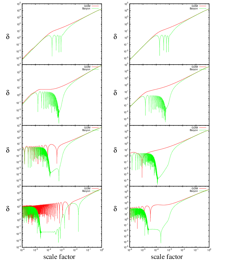
In Fig.4, we depict the evolutions of density perturbations of GDM with different wavenumbers ( Mpc-1) for two different model parameters ( eV and eV). We also depict those of the baryon density for comparison. At largest scales (top panels) the evolution of GDM density perturbations is almost identical to that of standard CDM, because the mode is always outside the sound horizon. On the other hand, the evolutions of the modes at small scales are depicted in the third and fourth panels. In these panels the amplitude of GDM exhibits oscillations when the perturbations are inside the sound horizon. The growth of density perturbation of GDM inside the sound horizon for is clearly seen, which has a dependence of as derived in our analytic estimate. We need, however, to see the second-top left panel ( Mpc-1 and eV) with care. The panel shows the marginal case where the mode exits the sound horizon immediately after entering the horizon. In this case, we observe that the amplitude of does not experience any logarithmic growth which is expected for the CDM case. We found that this brings a large difference in amplitudes at the present universe about an order of magnitude, which is seen by comparing with the second-top right panel.
The net effect in the matter power spectrum is the deficit of power for , which is shown in Fig.5. From this figure, we can find that the matter power spectrum alters not at as discussed in Sec.4.1, but at . That is because we have extended the analysis beyond the critical epoch in our numerical calculations, by extrapolating the behavior of GDM beyond with a reasonable assumption that the sound speed of GDM had been satulated as . In this case the density perturbation of GDM only oscillates inside the sound horizon and does not experience any logarithmic growth during the radiation dominated era which is expected in the CDM model. The power deficit at is more reasonable because it is a result derived mainly from the perturbation evolution at the subhorizon scales at the regime where the effective low-energy theory is applicable, i.e., or , under a simple assumption that the density perturbation of GDM can not grow deep in the radiation dominated era, even when the low energy effective theory is broken.
The evolution of the baryon density perturbation is affected only through gravity. In the standard cosmology, it is known that after the fluctuation is erased by diffusion damping the baryon fluctuation should start to grow in time again with terminal velocity falling into the gravitational potential of clustered dark matter [25]. In the GDM model, however, the baryon fluid can not have terminal velocity because the dark matter density fluctuation oscillates in the sound horizon and hence the gravitational potential. As the GDM ceases oscillating, the amplitude of the density fluctuation of baryon fluid starts growing with oscillation, which is clearly seen in the left bottom panel. In any case, the baryon density fluctuation quickly catches up the dark matter density one after decoupling.
The matter power spectrum of our universe can be probed through various cosmological observations, such as clustering of galaxies [26], cosmic shear [28, 27, 29], Lyman- forest [30, 31, 32], and so on. At present, almost all observational data support the CDM paradigm, roughly for the wavenumber Mpc-1. In the models considered in this paper, this observational fact gives us a constraint on the model parameter . The constraint is derived through the suppression of the matter power spectrum, in the same way to obtain the constraints on the hot and/or warm dark matter models (or in other words, masses of neutrinos and/or warm dark matter particles) [33]. By looking at the matter power spectrum obtained in the present analysis (Fig.5), we conclude that the model parameter should be
| (86) |
which is a stronger constraint than that obtained only from the background evolution considered in Sec. 3. This result is consistent with the rough analytic estimate given by Eq. (55).

Finally we should note that the way of suppression in the GDM models is different from that in hot or warm dark matter models. In the GDM models the suppression is the power law while for hot and warm models the power is exponentially suppressed. This fact might be used to distinguish between GDM and other dark matter models.
5 Summary and discussion
We have investigated the possibility that ghost condensation may serve as an alternative to dark matter, which had not been investigated in detail. In the present paper we have considered the GDM universe, i.e. a late-time universe dominated by a cosmological constant and ghost dark matter. We have investigated the Friedmann-Robertson-Walker (FRW) background evolution and the large-scale structure of the GDM universe, and have found a lower bound on the scale of spontaneous Lorentz breaking as . This bound is compatible with the phenomenological upper bound known in the literature.
As we have reviewed in Sec. 2, ghost condensation is the simplest Higgs mechanism for gravity in the sense that the number of Nambu-Goldstone boson is only one. The structure of the low-energy effective field theory is completely determined by the symmetry breaking pattern and this makes it possible for us to give robust predictions of the theory as far as the system is in the regime of validity of the effective theory. In Sec. 2 we have also reviewed the infrared modification of linearized gravity as well as some non-linear dynamics and the phenomenological lower bound mentioned above.
In Sec. 3 we have provided a simple description of ghost dark matter and investigated the FRW background evolution. In subsection 3.1 we have shown that, under a certain condition, the background evolution and the behavior of large-scale perturbations of ghost dark matter can be described by a fluid with the equation of state . This description has been used throughout this paper, except for numerical studies where the field picture turns out to be more convenient for some technical reasons. In subsection 3.2, as a possible cosmological scenario relating the late time evolution of ghost dark matter to the early universe, we have considered a generation mechanism of ghost dark matter at the end of ghost inflation [21]. In subsection 3.3 we have shown that the background FRW evolution in the GDM universe is indistinguishable from that in the standard CDM universe if .
In Sec.4 we have investigated the large-scale structure of the GDM universe. Since the GDM has the effective sound speed unlike the standard CDM, small scale perturbations are suppressed. The suppression of the matter power spectrum occurs in a way different from that in models with hot dark matter or warm dark matter particles. We have given an analytic treatment to predict the matter power spectrum observed today and have also calculated the power spectrum numerically. The analytic treatment can be extended for general dark matter models in which dark matter has a finite sound speed whose time dependence is the power law of scale factor. By comparing the GDM power spectrum with the observed one, one can get a lower bound on the scale . The result we obtained is .
The constraint obtained in this paper can be improved further by observations of the matter power spectrum at smaller scales. For example, 21cm-line observations and/or the precise determination of the reionization epoch will provide us plenty of information about the matter power spectrum at smaller scales and hence stronger limits on the ghost condensation scale . We leave these interesting subjects for future investigation.
As suggested in [11], ghost condensation may provide an alternative explanation for the acceleration of the present universe if . If the cosmological constant in the symmetric phase (with ) is zero then the effective cosmological constant in the broken phase, i.e. the ghost condensate, (with ) is positive 55 5 Note that in the standard Higgs mechanism, the effective cosmological constant in the broken phase would be negative if the cosmological constant in the symmetric phase is zero. and of order unless fine-tuned. Unfortunately, the condition is not compatible with the lower bound on found in the present paper under the assumption that ghost dark matter is responsible for all dark matter in the universe. Therefore, it is not easy for the ghost condensate to be a simultaneous alternative to dark energy and dark matter unless fine-tuned.
On the other hand, as shown in subsection 3.2, ghost inflation is compatible with ghost dark matter. Ghost dark matter is naturally produced at the end of ghost inflation. Moreover, the lower bound (46) from ghost inflation can be satisfied simultaneously with not only the phenomenological upper bound (29) but also the bound from ghost dark matter. Detailed investigation of the combination of ghost inflation and ghost dark matter is certainly worthwhile as a future work.
Acknowledgments.
We thank T. Chiba for informing us of a related work Ref. [22]. This research was supported by the Grant-in-Aid for Nagoya University Global COE Program, ”Quest for Fundamental Principles in the Universe: from Particles to the Solar System and the Cosmos”, by Grant-in-Aid for Scientific Research 21740177 (KI), 17740134 (SM), 19GS0219 (SM), 21111006 (SM), 21540278 (SM), by World Premier International Research Center Initiative (WPI Initiative), and by Grant-in-Aid for Scientific Research on Priority Areas No. 467 “Probing the Dark Energy through an Extremely Wide and Deep Survey with Subaru Telescope”, from MEXT of Japan.References
- [1] A. G. Riess et al. [Supernova Search Team Collaboration], Astron. J. 116, 1009 (1998) [arXiv:astro-ph/9805201].
- [2] A. G. Riess et al., Astron. J. 117, 707 (1999) [arXiv:astro-ph/9810291].
- [3] S. Perlmutter et al. [Supernova Cosmology Project Collaboration], Astrophys. J. 517, 565 (1999) [arXiv:astro-ph/9812133].
- [4] M. Kowalski et al. [Supernova Cosmology Project Collaboration], Astrophys. J. 686, 749 (2008) [arXiv:0804.4142 [astro-ph]].
- [5] M. Hicken et al., Astrophys. J. 700, 1097 (2009) [arXiv:0901.4804 [astro-ph.CO]].
- [6] E. J. Copeland, M. Sami and S. Tsujikawa, Int. J. Mod. Phys. D 15, 1753 (2006) [arXiv:hep-th/0603057].
- [7] G. Bertone, D. Hooper and J. Silk, Phys. Rept. 405, 279 (2005) [arXiv:hep-ph/0404175].
- [8] M. Fierz and W. Pauli, Proc. Roy. Soc. Lond. A 173, 211 (1939).
- [9] G. R. Dvali, G. Gabadadze and M. Porrati, Phys. Lett. B 485, 208 (2000) [arXiv:hep-th/0005016].
- [10] C. Deffayet, Phys. Lett. B 502, 199 (2001) [arXiv:hep-th/0010186].
- [11] N. Arkani-Hamed, H. C. Cheng, M. A. Luty and S. Mukohyama, JHEP 0405, 074 (2004) [arXiv:hep-th/0312099].
- [12] N. Arkani-Hamed, H. C. Cheng, M. A. Luty, S. Mukohyama and T. Wiseman, JHEP 0701, 036 (2007) [arXiv:hep-ph/0507120].
- [13] J. Garriga and V. F. Mukhanov, Phys. Lett. B 458, 219 (1999) [arXiv:hep-th/9904176].
- [14] S. Mukohyama, JCAP 0610, 011 (2006) [arXiv:hep-th/0607181].
- [15] M. L. Graesser, I. Low and M. B. Wise, Phys. Rev. D 72, 115016 (2005) [arXiv:hep-th/0509180].
- [16] D. O’Connell, Phys. Lett. B 643, 379 (2006) [arXiv:hep-th/0602240].
- [17] S. Mukohyama, JHEP 0705, 048 (2007) [arXiv:hep-th/0610254].
- [18] N. Bilic, G. B. Tupper and R. D. Viollier, JCAP 0809, 002 (2008) [arXiv:0801.3942 [gr-qc]].
- [19] S. Mukohyama, JHEP 0909, 070 (2009) [arXiv:0901.3595 [hep-th]].
- [20] S. Mukohyama, arXiv:0908.4123 [hep-th].
- [21] N. Arkani-Hamed, P. Creminelli, S. Mukohyama and M. Zaldarriaga, JCAP 0404, 001 (2004) [arXiv:hep-th/0312100].
- [22] D. Giannakis and W. Hu, Phys. Rev. D 72, 063502 (2005) [arXiv:astro-ph/0501423].
- [23] C. P. Ma and E. Bertschinger, Astrophys. J. 455, 7 (1995) [arXiv:astro-ph/9506072].
- [24] A. Lewis, A. Challinor and A. Lasenby, Astrophys. J. 538, 473 (2000) [arXiv:astro-ph/9911177].
- [25] K. Yamamoto, N. Sugiyama and H. Sato, arXiv:astro-ph/9709247.
- [26] M. Tegmark et al. [SDSS Collaboration], Phys. Rev. D 74, 123507 (2006) [arXiv:astro-ph/0608632].
- [27] J. Benjamin et al., Mon. Not. Roy. Astron. Soc., 381, 702, (2007) arXiv:astro-ph/0703570.
- [28] L. Fu et al., Astron. Astrophys. 479, 9 (2008) [arXiv:0712.0884 [astro-ph]].
- [29] T. Schrabback et al., arXiv:0911.0053 [astro-ph.CO].
- [30] R. A. C. Croft et al., Astrophys. J. 581, 20 (2002) [arXiv:astro-ph/0012324].
- [31] T. S. Kim, M. Viel, M. G. Haehnelt, R. F. Carswell and S. Cristiani, Mon. Not. Roy. Astron. Soc. 347, 355 (2004) [arXiv:astro-ph/0308103].
- [32] P. McDonald et al. [SDSS Collaboration], Astrophys. J. 635, 761 (2005) [arXiv:astro-ph/0407377].
- [33] A. Boyarsky, J. Lesgourgues, O. Ruchayskiy and M. Viel, JCAP 0905, 012 (2009) [arXiv:0812.0010 [astro-ph]].