Dusty winds — II. Observational Implications
Abstract
We compare observations of AGB stars and predictions of the Elitzur & Ivezić (2001) steady-state radiatively driven dusty wind model. The model results are described by a set of similarity functions of a single independent variable, and imply general scaling relations among the system parameters. We find that the model properly reproduces various correlations among the observed quantities and demonstrate that dust drift through the gas has a major impact on the structure of most winds. From data for nearby oxygen-rich and carbon-rich mass-losing stars we find that (1) the dispersion in grain properties within each group is rather small; (2) both the dust cross-section per gas particle and the dust-to-gas mass ratio are similar for the two samples even though the stellar atmospheres and grain properties are very different; (3) the dust abundance in both outflows is significantly below the Galactic average, indicating that most of the Galactic dust is not stardust—contrary to popular belief, but in support of Draine (2009). Our model results can be easily applied to recent massive data sets, such as the Spitzer SAGE survey of the Large Magellanic Cloud, and incorporated in galaxy evolution models.
Keywords:
stars: AGB and post-AGB — stars: late-type — stars: winds, outflows — stars: mass-loss — dust, extinction — infrared: stars —1 INTRODUCTION
Winds blown by stars on the asymptotic giant branch (AGB) are an important component of mass return into the interstellar medium and may account for a significant fraction of interstellar dust, including dust formation in the early universe (Sloan et al. 2009). Therefore in addition to its obvious significance for the theory of stellar evolution, the study of AGB winds has important implications for the structure and evolution of galaxies (Girardi & Marigo 2007; Marston et al. 2009). In our own Galaxy, its estimated 200,000 AGB stars are a good tracer of dominant components, including the bulge (Whitelock & Feast 2000; Jackson, Ivezić & Knapp 2002). AGB stars also have a great potential as distance indicators (Rejkuba 2004).
Over the past few years, data of AGB stars have improved significantly. The 2MASS survey delivered an all-sky near-IR photometric catalog to , and Spitzer obtained mid-IR (IRAC and MIPS) photometry for several thousand AGB stars from the Large Magellanic Cloud (LMC, Meixner et al. 2006). In addition, the MACHO survey provided high-quality light curves for 22,000 AGB stars from the LMC (Fraser et al. 2005), and the Northern Sky Variability Survey provided light curves for another 9,000 AGB stars brighter than and with declination (Woźniak et al. 2004). These new accurate and massive data sets are expected to rejuvenate studies of AGB stars, leading to model-based interpretation of diverse measurements including photometry, outflow velocity, mass-loss rate, pulsations, etc. (e.g., Marigo et al. 2008).
AGB stars are surrounded by an expanding envelope composed of gas and dust, that has a major impact on observed properties. The complete description of such a dusty wind should start with a full dynamic atmosphere model and incorporate the processes that initiate the outflow and set the value of . These processes are yet to be identified with certainty, the most promising are stellar pulsation (e.g. Bowen 1989; van Loon et al. 2008) and radiation pressure on the water molecules (e.g. Elitzur, Brown & Johnson 1989). Proper description of these processes should be followed by grain formation and growth, and subsequent wind dynamics. Two ambitious programs attempting to incorporate as many aspects of this formidable task as possible have been conducted over the last decade by groups at Berlin (see Winters et al. 2000; Wachter et al. 2008; and references therein) and Vienna (see Höfner 1999; Dorfi et al. 2001; Höfner et al. 2003; Nowotny et al. 2005; and references therein). While much has been accomplished, the complexity of this undertaking necessitates simplifications such as a pulsating boundary. In spite of continuous progress, detailed understanding of atmospheric dynamics and grain formation is still far from complete (e.g., Höfner & Andersen 2007).
Fortunately, the full problem splits naturally to two parts, as recognized long ago by Goldreich & Scoville (1976). Once radiation pressure on the dust exceeds all other forces, the rapid acceleration to supersonic velocities decouples the outflow from the earlier phases—the supersonic phase would be exactly the same in two different outflows if they had the same mass-loss rate and grain properties even if the grains were produced by entirely different processes. Furthermore, these stages are controlled by processes that are much less dependent on detailed micro-physics, and are reasonably well understood. And since most observations probe only the supersonic phase, models devoted exclusively to this stage should reproduce the observable results while avoiding the pitfalls and uncertainties of dust formation and the wind initiation.
In Elitzur & Ivezić (2001, hereafter paper I) we present the self-similarity solution of the dusty wind steady state supersonic phase. The model assumes steady-state spherically symmetric mass loss with prompt dust formation and no subsequent change in dust properties (i.e., no grain growth and sputtering). The included dynamical effects are the radiation pressure force, dust drift through the gas, and the gravitational pull by the star. Paper I contains the description of the model and its solution in full mathematical rigor. Here we discuss observational implications of the model, and compare them to available data. The main questions that we ask are
- •
Can the model explain the wind velocity profile, including the region of strong acceleration at small radii?
- •
Does the implied density profile produce spectral energy distributions in agreement with observations?
- •
Do dynamical quantities, such as the wind terminal velocity and mass-loss rate, and photometric quantities such as colors and bolometric flux, display correlations predicted by the model?
- •
How similar, or dissimilar, are dust properties inferred from observations of oxygen-rich and carbon-rich AGB stars?
We first discuss dynamical quantities, and then focus on the spectral energy distribution. In §2 we describe the wind velocity profile. Section 3 presents correlations among final velocity , mass loss rate and luminosity . In §4 we discuss the spectral energy distribution (SED) and its relationship with the wind dynamical properties. In §5 we discuss the allowed range of physical parameters of dusty winds. The results are summarized and discussed in §6. Equations from paper I are referred to by their number preceded by I.
2 Velocity Profile
The velocity profile for all winds, whether the dust is comprised of carbon or silicate grains, can be summarized with the simple analytic expression (see §3 in paper I)
| (1) |
Here is angular distance from the star in the plane of the sky and is a characteristic angular scale. The power introduces a weak dependence on , the overall radial optical depth at visual. The small- value reflects the effect of the drift, which dominates the dynamics in that regime. At large , reddening effects a switch to a more moderate profile with .
We discuss the wind terminal velocity in §3 below. Here we concentrate on the shape of the radial profile . The profile is mainly controlled by the characteristic angular scale , corresponding to the dust condensation radius. It can be determined from the measured bolometric flux, , via
| (2) |
Here is the dust condensation temperature and is a dimensionless function that sets the dust condensation radius as , where and are, respectively, the stellar radius and effective temperature. All our model calculations assume = 700 K and a black-body star with = 2500 K. The function is determined from the radiative transfer solution (see I.41 and I.42) and can be adequately approximated by the simple analytic expression
| (3) |
The parameters and are listed in Table 1 together with other relevant properties of the dust grains. In all the numerical calculations here we employ amorphous carbon grains with optical properties from Hanner (1988), and (the “warm” version of) silicate grains from Ossenkopf, Henning & Mathis (1992). We assume a single size = 0.1 m to compute the grain absorption and scattering efficiencies; the grain size does not enter the solution of the dusty wind problem in any other way. From their effect on the variation of angular scale with , the parameters and introduce the only dependence of the velocity profile on dust properties. However, in practice this effect is rather weak: varies by less than 10% for between 0 and 20.
| Carbon | Silicate | |
|---|---|---|
| 2.40 | 1.15 | |
| 0.60 | 0.11 | |
| 5.97 | 2.72 | |
| 1.0 | 1.25 |

We compare these model predictions with the spatially-resolved maser observations of three O-rich supergiants reported by Richards & Yates (1998). The combined measurements of SiO, H2O and OH masers trace the velocity profile over three orders of magnitude of radial distance from just outside the stellar atmosphere. Comparison with the theoretical profile in equation 1 requires three input parameters. The terminal velocity is measured directly in CO observations because most of the CO emission comes from the outer parts of the envelope, far beyond the acceleration zone. Next, we constrain the optical depth, , which controls the power-law index , by fitting the spectral energy distributions, as described below in §5 (its effect on is minor). Finally, we determine the angular scale from eq. 2 and the measured . In using this relation we assumed = 700 K for all three stars, but the entire range 600–800 K is consistent with the data. All relevant parameters for the three stars are listed in table 2 and the resulting are shown in figure 1. With parameters constrained only by photometric and CO observations, the model successfully predicts the velocity profiles measured from the independent maser observations. The good agreement is obtained even though the model profiles were not fitted to the data with any adjustable free parameters. This supports the prediction given by eq. 1, as well as the vs. relationship given by eq. 2.
| Star: | S Per | VY CMa | VX Sgr | source |
| Measured: | ||||
| Spec. Type | M3I | M3/M4II | M5/M6III | a |
| (kpc) | 2.3 | 1.5 | 1.5 | b |
| () | 20 | 50 | 10 | b |
| ( yr-1) | 2.7E5 | 1.0E4 | 2.5E5 | b |
| (W/m2) | 5.1E10 | 6.6E9 | 2.3E9 | c |
| ( ) | 8.1 | 44 | 16 | d |
| (km s-1) | 19.7 | 44.0 | 26.0 | e |
| LRS class | 26 | 24 | 26 | f |
| 0.16 | 0.17 | 0.29 | f | |
| 0.76 | 0.66 | 0.72 | f | |
| Model: | ||||
| (mas) | 30 | 110 | 65 | |
| 3.2 | 18.0 | 5.6 |
3 Correlations among Dynamical Quantities
Specifying the dust chemical composition determines its optical properties, with the relevant parameters listed in table 1. An additional, independent property is the dust abundance, conveniently parametrized with the dust cross-sectional area per gas particle upon grain condensation
| (4) |
that is, and are the number densities of hydrogen nuclei and dust particles, respectively, before the drift sets in (see paper I, eq. 5). The cross-section is a free parameter that controls the relation between optical depth, mass-loss rate and luminosity as (paper I, eq. 55)
| (5) |
where = , and with . While has no bearing upon the shape of the radial profile , it sets the scale of the outflow terminal velocity, which is related to and as (paper I, eq. 52)
| (6) |
where . Combining eqs. 5 and 6, it is evident that when is varied at a fixed , the terminal velocity reaches maximum when = 1, i.e., at a mass loss rate . From this maximum, decreases when is either increasing or decreasing away from . This decrease reflects the role of the drift in one direction, reddening the other.
3.1 Drift-dominated regime


When decreases away from so that becomes less than unity, the dust and gas decouple and the velocity decreases too. In this drift dominated regime11 1 For grains smaller than about 0.01 m, the dust drift can be negligible even when ; for discussion see Section C1 in paper I., eq. 6 becomes
| (7) |
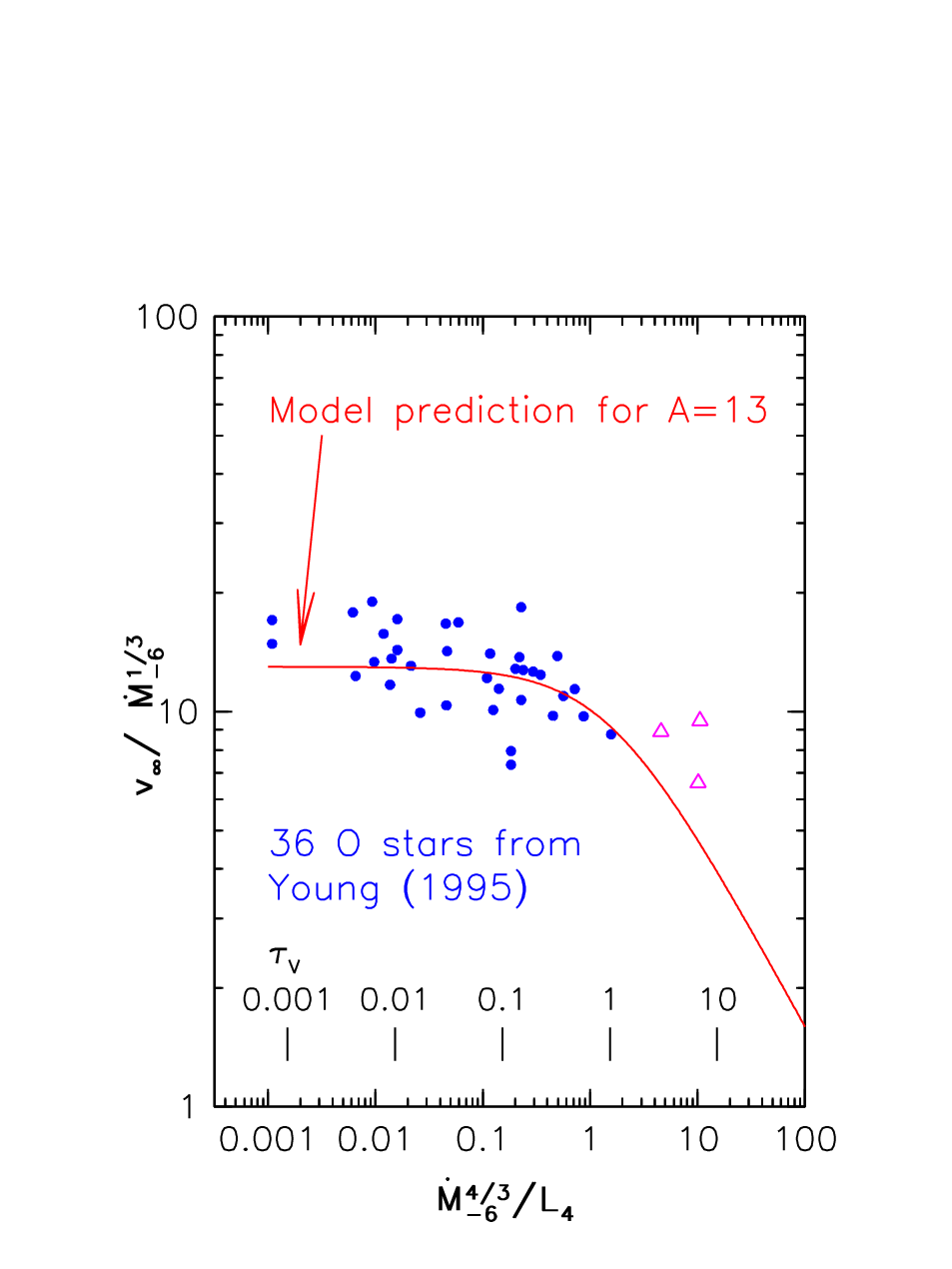
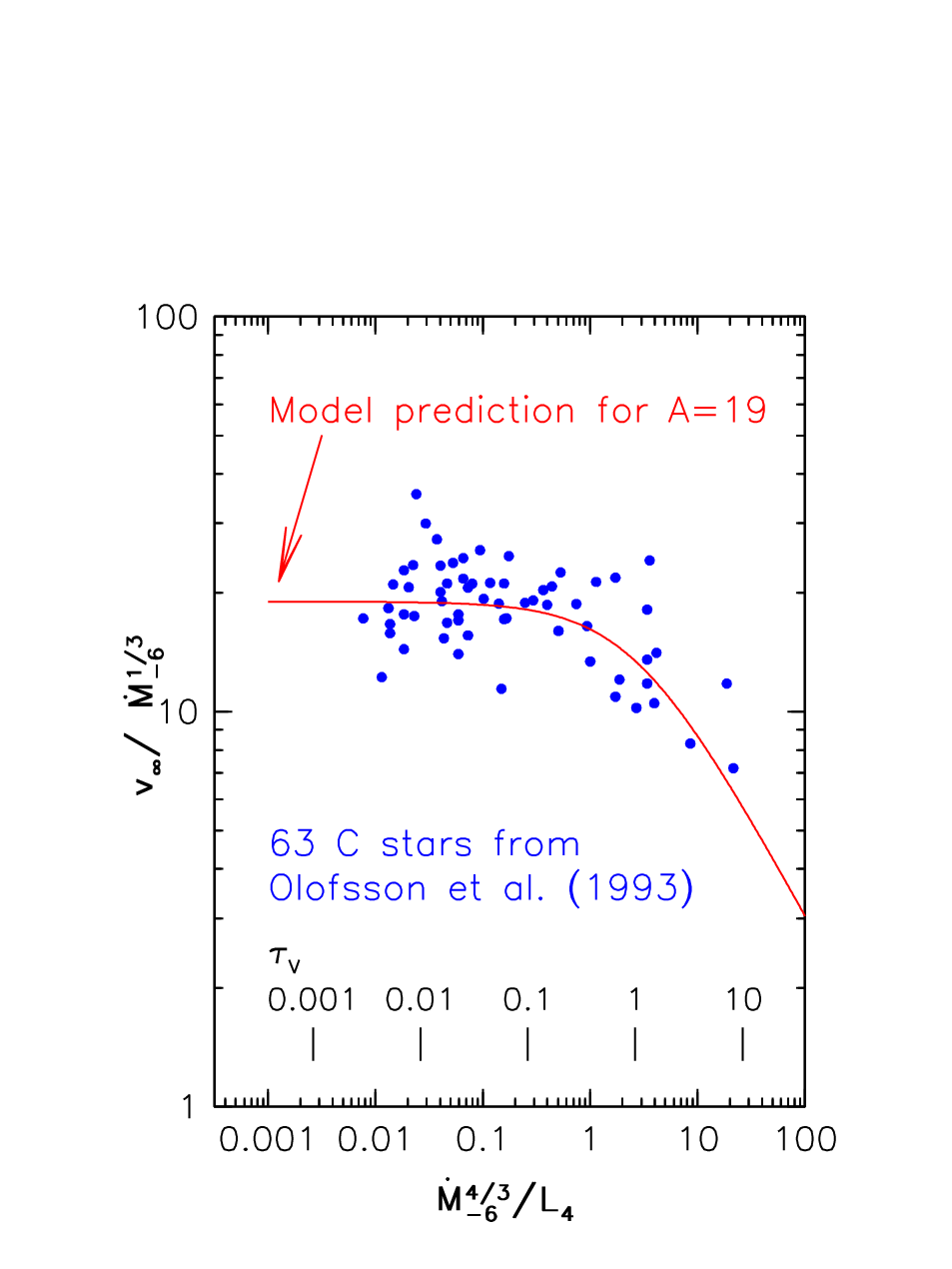
It is remarkable that, even though the wind is driven by radiation pressure, its velocity is independent of luminosity for small (optically thin limit; see also §4.2 in paper I). This surprising result was discovered observationally by Young (1995) in a survey of 36 nearby Mira variables with low mass-loss rates. Young found a clear, strong correlation between outflow velocity and mass-loss rate, but independent of luminosity. His correlation can be parametrized as , in agreement with eq. 7 if the observational errors for the power-law index are at least 10%, which is plausible. Figure 2 presents Young’s data as a histogram of . The figure also lists the distribution mean and its root-mean-square scatter , and plots the Gaussian with these parameters. Figure 3 presents a similar analysis of C-rich stars with small optical depths, with data from Olofsson et al. (1993). In the case of Young’s data we did not introduce any cuts since the sample is dominated by optically thin envelopes, as can be seen from figure 5. On the other hand, the 63 C-rich stars in the Olofsson et al data include three objects with , as is evident in figure 6, and these were excluded from the histogram. Each histogram shows a pronounced peak—in agreement with eq. 7 when the dust properties do not vary much within the sample. The ratio is for each sample, a fractional scatter consistent with the measurement errors (10% for and 50% for ; see Appendix for details). These strongly peaked distributions affirm the central role of dust drift at small mass loss rates and indicate a close similarity of dust properties within each sample.
3.2 Dust-to-gas ratios
The velocity scale , 19 km s-1 for C-rich and 13 km s-1 for O-rich stars, is a fundamental property of dusty winds, derived directly from the data. Adding assumptions regarding the grain properties enables determination of the dust geometric cross-section per gas particle from
| (8) |
where . The top panel of figure 4 shows the variation with grain size of the inferred values of for amorphous carbon and silicate grains. Remarkably, the two samples of different type stars produce values of that agree to within 50% at all grain sizes. In spite of the large differences in atmospheric and grain properties between O- and C-rich stars, the fraction of material channelled into dust is such that the dust area per gas particle turns out to be roughly the same in both.
The quantity closest to that is directly determined in observation is the dust extinction per H column density. The Galactic average yields cm-2 (e.g., Sparke & Gallagher 2006), which translates to = 5. The middle panel of figure 4 shows the variation with grain size of the value of inferred from the measured values of for the C- and O-rich stars. Galactic interstellar dust contains a mixture of carbon and silicate grains of various sizes, but the dusty wind results are significantly below the Galactic average for both types of dust and any grain size; averaging the results with the MRN (Mathis, Rumpl & Nordsieck 1977) size distribution yields the values indicated in the figure with dot-dashed lines.
Another indicator of dust abundance is the dust-to-gas mass ratio ; it is widely used even though its determination invokes assumptions about molecular abundances that bring additional uncertainty. Estimates of the Galactic average of range from 0.005 (Draine 2009) to 0.01 (Barbaro et al 2004). Recalling that characterizes the base of the outflow where the gas and dust have the same velocity (prior to the dust drift; see eq. 4), the outflow dust-to-gas mass ratio is
| (9) |
where is the density of the grain material (3.28 g cm-3 for silicate dust, 2.2 g cm-3 for carbon grains). The bottom panel of figure 4 shows the variation with grain size of the value of for dusty winds, providing yet another display of two properties noted above: (1) In spite of the large differences in their formation properties, the mass fraction of carbon and silicate grains is roughly the same in both types of stars, and (2) the wind dust abundance is significantly below the Galactic average.
These results have significant consequences regarding the origin of interstellar dust. Using either or as indicators, the dust abundance in winds around evolved stars is substantially lower than the Galactic averages irrespective of grain size or chemical composition. The MRN average for in dusty winds is more than a factor of 10 below the Galactic average for silicate dust, a factor of 5 for carbon. Since the winds fail to produce the observed ISM values for both types of grains at all sizes, mixture averaging cannot bring the results to the Galactic values. The implication is that dusty winds cannot be the source of all Galactic dust: If all dust were formed by cycling interstellar gas through stars, with existing grains destroyed during star formation and reformed around evolved stars, than the Galactic average could not exceed the dusty winds value. Draine (2009) discusses additional grain destruction mechanisms in estimating the Galactic dust budget, and concludes that they could not be offset by formation in stars (see also Zhukovska, Gail & Trieloff 2008). Our results show that even without considering any processes other than cycling through stars, most interstellar dust is not stardust and must have formed in the ISM, in strong support of Draine’s conclusion.
It should be noted that the analysis here provides a robust derivation of the dust abundance. The parameter is determined directly from the data, and its conversion to and involves only minimal assumptions about the grain properties; significantly, no assumptions are made about any molecular abundances. The presented results employed = 700 K, and the inferred dust abundance scales as . Varying in its likely range, the dust abundance would increase at every by 36% for = 600 K and decrease by 23% if = 800 K; such variations have little effect on our conclusions. In addition, there is no need to consider global balance of dust forming and destruction processes in the ISM, which are very uncertain. Our conclusion is derived from consideration of individual stars and therefore it is independent of, and supports, Draine’s arguments.

3.3 Optically thick winds
As increases away from , the wind becomes optically thick and reddening degrades the efficiency of the radiation pressure force, thus the velocity again decreases. The wind velocity is no longer independent of luminosity. Instead, from equations 6 and 5 it follows that when , the final velocity is proportional to . Therefore, the ratio is no longer constant, instead it decreases as from its value in the optically thin regime. Figures 5 and 6 show the comparison of model predictions with observations, by plotting the data and the relationship in eq. 6 in the plane. Since the single free parameter is taken from the histograms in figures 2 and 3, the agreement between model and data displayed in figures 5 and 6 is obtained without adjusting any parameters; the coefficient controls both the constant asymptotic value of in the small regime as well as the value of at which begins to decrease, thus this agreement represents another test of the model. This test would be much stronger if the samples contained more stars with very large values of (i.e., ) so that the transitions from optically thin to thick regimes were better defined. We note that the samples are dominated by optically thin envelopes, thus our above estimates of the mean are not appreciably biased by the few stars with moderate optical depths.
4 Physical Domain of Dusty Winds
The relation has often been invoked as the momentum conservation bound on radiatively driven mass loss rates, even though the mistake in this application when has been pointed out repeatedly (e.g. Ivezić & Elitzur 1995). Instead, the proper form of momentum conservation is , where is the flux-averaged optical depth. Since can exceed unity for plausible values of (see paper I, eq. 57 and figure 6), momentum conservation does not impose a meaningful constraint on dusty winds. Instead, the constraints come from force considerations—the radiative outward force must exceed everywhere the gravitational pull of the star with mass . This condition breaks down at the two ends of the mass-loss-rate range, where the outward force is reduced for two different reasons: at very low the gas–dust momentum coupling weakens thus reducing the force on the gas, and at very high the coupling to the radiative force diminishes because of the enhanced reddening that follows increased obscuration. In paper I (see sec. 5, in particular figure 7) we derive the resulting phase-space boundaries with the aid of the appropriate scaling variables. Here we reproduce the results in terms of the system physical parameters.
Figure 7 shows the lower bound on , arising from the requirement that radiation pressure on the dust should provide sufficient force on the gas to generate a net acceleration at the base of the outflow. This liftoff condition sets a lower bound on , proportional to (paper I, eq. 69); below this minimal the grains are ejected without dragging the gas with them because the density is too low for efficient gas–dust coupling. As a condition on the wind initiation, this bound is the most uncertain part of our solution. The result is reasonably secure (a similar relation was noted by Habing et al 1994), but the proportionality constant can be determined accurately only from a more complete formulation that handles properly grain growth and the wind launching mechanism.
The bound shown in figure 8 reflects the weakening of radiative coupling in optically thick winds because of the radiation reddening. For any Eddington ratio (the horizontal axis), the figure shows the upper limit on the wind optical depth (; see eq. 5), determined from the full numerical solution of the self-similar problem; the vertical axis units were chosen to vary linearly with . Although some stars have , none violate the upper bound set by proper solution of the dusty wind problem.


5 The Wind IR Emission
Given the grain properties, the dusty wind problem requires three independent input parameters, which can be selected as the initial velocity, the Eddington ratio and the overall optical depth (paper I). However, the dependence on the first two is limited to the immediate vicinity of the boundary of the phase-space for physical solutions; away from that boundary, dusty winds are described by a set of similarity functions of the single independent variable . Figures 7 and 8 show that most stars are located well inside the allowed region of phase space and thus should be well described by alone. Therefore, we should be able to characterize every property of the wind IR emission (SED, colors, etc.) with only.
We employed the code DUSTY (Ivezić, Nenkova & Elitzur 1999) to compute the SED of each of the three oxygen-rich stars whose velocity profiles, as well as the approximate analytic solution of eq. 1, are shown in figure 1. The DUSTY calculations were done using the code’s option “analytic radiatively driven wind”, which computes the density profile from the same approximate analytic solution (for details, see the DUSTY manual). Figure 9 shows the model SEDs, fitted to the data with the single free parameter . The same models that successfully explain the velocity profiles measured from maser observations also produce satisfactory fits to SED of each star. The best-fit values for are listed in table 2. Another example where SED fits provided successful predictions for the spatially resolved velocity profile is W Hya. Zubko & Elitzur (2000) fitted simultaneously the SED and the velocity profile deduced from observations of the CO thermal emission and various masers. Significantly, neither nor or dust-to-gas ratio were input parameters in that model. Instead, these quantities were derived from general self-similarity relations after the SED fitting results were supplemented by the distance and velocity scales.
Successful SED fitting is not limited to stars with silicate dust. We have shown elsewhere that the SED of the very dusty carbon-rich star IRC+10216 can be fitted as a function of pulsation phase by simply varying optical depth (Ivezić & Elitzur 1996).


5.1 A Comment on Estimating Mass-loss Rate from IR Observations
The infrared emission from dust is related to the gas mass-loss rate and may offer observationally convenient way to estimate the latter. The literature is abundant with various proposed expressions that relate IR observables and mass-loss rate (e.g. van Loon 2008, and references therein; see also van der Veen & Rugers 1989). However, in addition to heterogeneous data sets and methods (see Appendix for a summary), it is often unclear what assumptions are made, and what variables are considered to be independent. A key point of our analysis is that there are only two independent relations between various relevant quantities, and they reflect energy and momentum conservation (eqs. 5 and 6). Given these two relationships, only two quantities can be derived, and all others have to be assumed, or measured. Thanks to its scaling properties, the problem of connecting gas mass-loss rate to IR observables can be decoupled into two independent steps: determination of from IR observables, and relating to dynamical quantities, including gas mass-loss rate.
The most robust and accurate method for estimating from observations is fitting of a well-sampled SED. When the data are sparse, various IR colors can also be used, albeit with deteriorating accuracy. Examples of such relationships are show in figure 10. Given an estimate of , the model uniquely predicts correlations between and various combinations of dynamical quantities formed using , , , and . Examples of such relations are shown in figure 11 (based on eqs. 5 and 6, as well as , with the latter derived from, and not independent of, the first two expressions). The most appropriate expression to use for estimating gas mass-loss rate depends on the available data. For example, in case of the LMC studies, where outflow velocity is available for a much smaller number of stars than photometry, eq. 5 provides a superior approach because it involves only SED fitting (distance to the LMC can be considered well constrained in this context): for fixed values of and , only and are required to estimate . The values for and (see definitions after eq. 5) can be taken as equal to the Galactic case (Table 1), or could be determined as in Section 3.1 using a sample of LMC stars with outflow velocity and mass-loss rate measurements.

6 DISCUSSION
We have presented here a summary of the Elitzur & Ivezić (2001) similarity solution in terms more suitable for direct comparison with observations. The correlation of and in optically thin winds (eq. 7), first discovered observationally by Young (1995), emerges as a fundamental property of radiatively driven dusty winds and a powerful tool in the analysis of their data. Our own analysis in §3.1 uncovers two major new results: (1) The peaked distributions in figures 2 and 3 indicate there is little variation in dust properties among O-rich and C-rich stars, and (2) the dust cross section per gas particle () and the dust-to-gas mass ration () are essentially the same for the two classes. It is hard to think of another method that could produce these conclusions with a similar level of confidence. Both of these results present a major challenge for theoretical studies of dust formation.
The relatively small scatter around Young’s correlation suggests also a new method for determining mass-loss rates in optically thin outflows from the relation
| (10) |
where is in km s-1 and is from §3.1. Here is determined from the single measurement of , without any assumptions about dust abundance. In addition, there is no distance dependence, nor any need for complex modeling. The scatter in this relation is expected to be 50-70%, no worse than any other method for determining mass loss rates (see Appendix A). The only restriction is that the wind optical depth at visual must be less than unity, a condition that is easy to verify observationally. Of course, the absolute uncertainty of scale is inherited from Young’s (1995) calibration of his CO measurements, via the values of the parameter.
In the broader context of Galactic ISM dust, our analysis represents independent support for Draine’s (2009) conclusion that most ISM dust particles were formed in situ, rather than produced in AGB winds. If verified, this conclusion would have important consequences for our understanding of galaxy evolution.
Our model captures all the scaling relationships among the main observable quantities that follow from energy and momentum conservation. These correlations can be used to estimate quantities whose measurements might not be available, notably the mass-loss rate, and for modeling the impact of AGB stars on their host galaxies. An example is the recent extensive modeling study by Marigo et al. (2008). Our results are also suitable for analysis of massive data sets such as the recent SAGE survey of the LMC (Meixner et al. 2006). We emphasize that our derived values of and are directly proportional to the ratio in the optically thin domain. If one wished to compare for two populations of stars, say from the Galaxy and the LMC, a robust method is to compare the distributions for samples verified to be optically thin using spectral energy distribution.
Despite the successful confrontation of our model with observations, reality is more complex. The model assumes steady state and spherical geometry, but there is evidence that in some stars mass-loss rate is not steady (see, e.g., Marengo, Ivezić & Knapp 2001, and references therein) and that some contain an additional bipolar component (see, e.g., Vinković et al 2004, and references therein). In addition, the physical and chemical details at the base of the acceleration region are not included in our model. It would be prudent to compare predictions for the velocity spatial profile and relationships among dynamical and spectral quantities produced by more elaborate models, e.g., Fleischer, Winters & Sedlmayr 1999, Höfner 1999 and Dorfi et al 2001. Such a comparison would help identify which features in these complex models are simply direct consequences of energy and momentum conservation, and which are unique to detailed modeling of various physical and chemical effects.
Acknowledgments
We thank Jill Knapp and Bruce Balick for illuminating discussions. The partial support of NASA and NSF is gratefully acknowledged.
References
- [2] Barbaro, G., Geminale, A., Mazzei, P., & Congiu, E. 2004, MNRAS, 353, 760
- [4] Bowen, G.H 1989, in “Evolution of peculiar red giant stars”, Proceedings of the 106th IAU Colloquium, Bloomington, IN, July 27-29, 1988 (A90-31201 12-90). Cambridge and New York, Cambridge University Press, p. 269-283.
- [6] Draine, B. T. 2009, arXiv:0903.1658
- [8] Elitzur, M., Brown, J.A. & Johnson, H.R. 1989, ApJ, 341, L95
- [10] Elitzur, M., & Ivezić Ž. 2001, MNRAS, 327, 403 (Paper I)
- [12] Gezari, D.Y., Schmitz, M., Pitts, P.S., & Mead, J.M. 1993, Catalogue of Infrared Observations (NASA Reference Publication 1294)
- [14] Girardi, L. & Marigo, P. 2007, ASPC 378, 7
- [16] Habing, H. 1996, A&A Rev., 7, 97
- [18] Habing, H.J. et al. 1985, A&A, 151, L1
- [20] Habing, H.J., Tignon, J. & Tielens, A.G.G.M. 1994, A&A 286, 523
- [22] Hanner, M.S. 1988, NASA Conf. Pub. 3004, 22
- [24] Höfner, S. 1999, A&A, 346, 9
- [26] Höfner, S., Gautschy-Loidl, R., Aringer, B. & Jorgensen, U.G. 2003, A&A, 399, 589
- [28] Höfner, S. & Andersen, A.C. 2007, A&A, 465, 39
- [30] Ivezić Ž., & Elitzur M., 1995, ApJ, 445, 415
- [32] Ivezić Ž., & Elitzur M., 1996, MNRAS, 279, 1019
- [34] Ivezić, Ž., Nenkova, M., & Elitzur, M., 1999, User Manual for DUSTY, University of Kentucky Internal Report, accessible at http://www.pa.uky.edu/moshe/dusty
- [36] Jackson, T., Ivezić, Ž., & Knapp, G.R. 2002, MNRAS, 337, 749
- [38] Jura, M., 1987, ApJ, 313, 743
- [40] Knapp, G.R., & Morris, M. 1985, ApJ, 292, 640
- [42] Knauer, T.G., Ivezić, Ž., & Knapp, G.R. 2001, ApJ, 552, 787
- [44] Marengo, M., Ivezić, Ž., & Knapp, G.R. 2001, MNRAS, 324, 1117
- [46] Marigo, P., Girardi, L., Bressan, A., et al. 2008, A&A, 482, 883
- [48] Marston, C., Strömbäck, G., Thomas, D., Wake, D.A. & Nichol, R.C. MNRAS 394, 107 (2009).
- [50] Mathis J.S., Rumpl W. & Nordsieck K.H. 1977, ApJ, 217, 425
- [52] Nowotny, W., Lebzelter, T., Hron, J. & Höfner, S. 2005, A&A, 437, 285
- [54] Olofsson, H., Eriksson, K., Gustafsson, B. & Carlstrom, U. 1993, ApJS, 87, 267
- [56] Olofsson, H. 1996, Ap&SS, 245, 169
- [58] Olofsson, H. 1997, in IAU Symp. 178, The Carbon Star Phenomenon, ed. R.F. Wing (Dordrecht: Kluwer), p. 457-468
- [60] Ossenkopf, V., Henning, Th. & Mathis, J.S. 1992, A&A, 261, 567
- [62] Rejkuba, M. 2004, A&A, 413, 903
- [64] Richards, A.M.S. & Yates, J.A. 1998, IrAJ, 25, 7
- [66] Skrutskie, M.F. et al. 1997, The Impact of Large-Scale Near-IR Sky Surveys, ed. F. Garzon et al. (Dordrecht: Kluwer), 25
- [68] Sparke, L. S., & Gallagher, J. S., III 2006, Galaxies in the Universe – 2nd Edition, Cambridge University Press.
- [70] Sloan G.C., Matsuura, M., Zijlstra, A.A., et al. 2009, Science, 323, 353
- [72] van der Veen, W.E.C.J., & Rugers, M. 1989, A&A, 226, 183
- [74] van Loon, J.Th. 2008, Mem. S.A.It., 79, 412
- [76] van Loon, J.Th., Cohen, M., Oliveira, J.M., et al. 2008, A&A, 487, 3
- [78] Vinković, D., Blöcker, T., Hofmann, K.-H., et al. 2004, MNRAS, 352, 852
- [80] Wachter, A., Winters, J.M., Schröder, K.P. & Sedlmayr, E. 2008, A&A, 486, 497
- [82] Wallerstein, G. & Knapp, G.R. 1998, ARA&A, 36, 369
- [84] Winters, J.M., Le Bertre, T., Jeong, K.S., Helling, Ch. & Sedlmayr, E. 2000, A&A, 361, 641
- [86] Whitelock, P.A. & Feast, M.W. 2000, MNRAS 317, 460
- [88] Whitelock, P.A., Marang, F. & Feast, M.W. 2000, MNRAS 319, 728
- [90] Woźniak, P.R., Williams, S.J., Vestrand, W.T. & Gupta, V. 2004, AJ, 128, 2965
- [92] York, D.G., Adelman, J., Anderson, S., et al. 2000, AJ, 120, 1579
- [94] Young, K. 1995, ApJ, 445, 872
- [96] Zhukovska, S., Gail, H.P. & Trieloff, M. 2008, A&A, 479, 453
Appendix A Summary of Observations
Here we summarize the main measuring methods for most relevant observables, with emphasis on their accuracy and scaling with distance.
A.1 Dynamical Quantities
Observational methods for determining mass-loss rate and outflow velocity were analyzed and compared by van der Veen & Rugers (1989, hereafter vdVR). More detailed discussions are presented by Habing (1996), Olofsson (1996, 1997) and Wallerstein & Knapp (1998). There are three widely employed methods:
- •
The strength and shape of thermal CO line profiles contain information about the outflow velocity and the total amount of CO in the circumstellar shell. The shape and width of the line profile constrains the outflow velocity in an almost model-independent way. With the current observational capabilities and moderate signal-to-noise ratios, the outflow velocity can be constrained to better than 10%. Most of the CO emission comes from the outer parts of the envelope, and thus the measured velocity usually corresponds to the final outflow velocity.
The relationship between the implied CO mass and the directly observed quantities is a complex model-dependent function. The expressions most often used in data analysis were derived by Knapp & Morris (1985). The transformation from the CO mass to gas mass-loss rate requires further assumptions about the outflow, its geometry, and the CO-to-gas ratio. Assuming a steady-state outflow and spherical geometry, vdVR derive expressions that can be used to estimate gas mass-loss rate with an uncertainty of about a factor 2-5. More accurate estimates can be obtained by detailed modeling of individual sources, but probably not significantly better than a factor of 2. We note that the mass-loss rate estimate scales with , where is the source distance.
- •
The OH(1612MHz) maser line profile contains information about the outflow velocity and the amount of OH molecules. The line profile usually has two well-defined peaks whose velocity separation typically constrains the outflow velocity to better than 10%. This estimate is less model-dependent than the estimate based on the CO line profile, but unfortunately can only be used for oxygen-rich (O) stars.
Baud & Habing (1983) proposed a simple model-dependent relation that can be used to estimate the mass-loss rate from the peak flux of OH emission. As pointed out by vdVR, the uncertainty of this estimate can be as large as a factor of 5 due to strong temporal variations in the OH emission strength. Intrinsic accuracy of this method is probably not much better than a factor of 2 due to a number of assumptions made, and due to uncertain values of the OH-to-gas ratio. We note that the mass-loss rate estimate proposed by Baud & Habing scales with .
- •
The third widely employed method for estimating mass-loss rate is based on infrared observations of dust emission. The proposed expressions (Herman et al. 1986, Jura 1987) relate the observed emission to the optical depth, which in turn is assumed to encode information about the gas mass-loss rate and outflow velocity. Similarly to the above two methods that rely on the assumptions about the CO-to-gas and OH-to-gas ratios, the infrared-based mass-loss rate estimate is greatly affected by uncertain dust-to-gas ratio. Depending on numerous additional assumptions employed by various authors, the distance dependence of the infrared mass-loss rate estimates varies from proportional to , to no dependence at all.
Various observables that relate infrared emission to optical depth have been also been widely utilized. Both Herman et al. and Jura assume that the 60 m dust emission is optically thin, leading to , where is the IRAS flux at 60 m and is the bolometric flux. Van der Veen and Rugers (vdVR) relate the optical depth to the flux ratio, where and are the IRAS fluxes at 12 and 25 m.
One of the most widely used prescriptions for determining mass-loss rate from IR observations was proposed by Jura (1987). He assumed that the dust mass-loss rate is proportional to dust outflow velocity and dust optical depth, and that dust outflow velocity is proportional to gas outflow velocity. Dust optical depth is assumed to be linearly proportional to the far-IR flux (IRAS 60 m bandpass) because both the dust optical depth and the stellar contribution to the overall flux are very small at such long wavelengths. Given the importance of dust drift in optically thin regime discussed in §3.1, the success of Jura’s formula is very surprising: for small optical depths the ratio of dust and gas velocities is much larger than unity, which should lead to significant underestimate of mass-loss rate.
It turns out that there are two effects that offset each other, and the Jura’s expression for coincidentally produces correct values over a large dynamic range of mass-loss rate. In addition to neglected dust drift, the assumption about far-IR flux being dominated by dust emission also breaks down in optically thin regime. These effects are quantitatively illustrated in figure 12: at small mass-loss rates the increase of the ratio of dust and gas velocities is well matched by the decrease of the dust emission contribution to the 60 m flux. As a result, Jura’s mass-loss rate estimate never deviates by more than a factor of 2 from the median mass-loss rate ratio shown by the dotted line in figure 12 (this median ratio is 2.5 and represents an overall systematic offset of two mass-loss rate scales). Hence, the success of Jura’s formula, which does not incorporate dust drift, is not an argument against our model which includes dust drift.

Figure 12: The ratio of mass-loss rate given by our model and that derived using Jura’s formula is shown by the solid line, as a function of the former. The ratio of dust and gas velocities is shown by the dashed line, and the ratio of 60 m dust emission and total flux (i.e. including the stellar contribution) is shown by the dot-dashed line. As a result of the opposite trends, Jura’s formula is coincidentally correct to within a factor of 2 over a large range of mass-loss rate. The horizontal lines are added to guide the eye and represent the median ratio in the range 10-8 to 10-4 yr-1 (dotted line) and 10-7 to 10-4 yr-1 (thin solid line).
A.2 Photometric Quantities
The dusty envelope absorbs the stellar radiation and reradiates it at longer
wavelengths, thus making the infrared emission the most important part of the SED for model testing. The largest catalog of infrared observations is compiled by Gezari et al. (1993). Individual fluxes may often be more accurate than 10%, but due to the inhomogeneous nature of the catalog, the mean overall accuracy is probably lower. The wavelength coverage greatly varies among the sources and often is based only on the IRAS catalog. Recent large scale sensitive digital surveys (e.g. infrared 2MASS, Skrutskie et al. 1997; optical SDSS, York et al. 2000) are bound to significantly improve the availability of accurate multi-wavelength photometry.
Given the photometric data accurate to within 10%, the bolometric flux could be determined with the same accuracy, at least in principle. In practice, however, the wavelength coverage can be sparse and this shortcoming can lead to severe errors, unless the shape of SED is known a priori. Another difficulty is the variability of AGB stars which can also contribute significantly to bolometric flux errors. Given all these uncertainties, the bolometric flux can be determined to better than 20-30% only for a small number () of well observed stars.
A.3 Distance
Several methods are employed to estimate distances to AGB stars. The simplest one assumes that all AGB stars have luminosity of 104 , and determines distance using bolometric flux. Apart from a bias in this estimate (the median AGB luminosity is at least a factor of 2 smaller, see e.g. Habing et al. 1985, and Knauer, Ivezić & Knapp 2001), its intrinsic accuracy cannot be better than about 20-30% due to the finite width of the AGB luminosity function (Jackson, Ivezić & Knapp 2002). Other methods that have been frequently used to estimate distance include period-luminosity relations (e.g., Whitelock, Marang & Feast 2000), assumption that the absolute K-band magnitude is the same for all stars, and kinematic estimates based on radial systemic velocities. The distance errors associated with these methods are hard to characterize and sometimes do not even have a Gaussian distribution (e.g. kinematic distances); they may be more accurate than a factor of two, but probably not better than 20-30%.
The distance estimates to nearby AGB stars have been recently greatly improved with the data obtained by the HIPPARCOS satellite. The accuracy of HIPPARCOS distances varies from a star to star, but, nevertheless, there are now hundreds of AGB stars with distance estimates better than 10%.
A.4 Bolometric Luminosity
The bolometric luminosity can be determined using the bolometric flux and distance estimates. Assuming HIPPARCOS distances and stars with good photometric coverage, the luminosity can determined to within 10-20%. In more typical cases, its uncertainty is closer to 50% (e.g. Knauer, Ivezić & Knapp 2001), and without a Hipparcos parallax it can be as large as a factor of 2 (Jackson, Ivezić & Knapp 2002).