Planck pre-launch status: Low Frequency Instrument calibration and expected scientific performance
Abstract
We give the calibration and scientific performance parameters of the Planck Low Frequency Instrument (LFI) measured during the ground cryogenic test campaign. These parameters characterise the instrument response and constitute our best pre-launch knowledge of the LFI scientific performance. The LFI shows excellent stability and rejection of instrumental systematic effects; measured noise performance shows that LFI is the most sensitive instrument of its kind. The set of measured calibration parameters will be updated during flight operations through the end of the mission.
Key Words.
Cosmic Microwave Baground, Cosmology, Space Instrumentation, Coherent Receivers, Calibration and Testing1 Introduction
The Low Frequency Instrument (LFI) is an array of 22 coherent differential receivers at 30, 44, and 70 GHz on board the European Space Agency Planck11 1 Planck (http://www.esa.int/Planck) is a project of the European Space Agency - ESA - with instruments provided by two scientific Consortia funded by ESA member states (in particular the lead countries: France and Italy) with contributions from NASA (USA), and telescope reflectors provided in a collaboration between ESA and a scientific Consortium led and funded by Denmark. satellite. In 15 months22 2 There are enough consumables on board to allow operation for an additional year. of continuous measurements from the Lagrangian point Planck will provide cosmic-variance- and foreground-limited measurements of the Cosmic Microwave Background temperature anisotropies by scanning the sky in near great circles with a 1.5 m dual reflector aplanatic telescope (Tauber 2009; Martin et al. 2004; Villa et al. 2002; Dupac & Tauber 2005).
The LFI shares the focal plane of the Planck telescope with the High Frequency Instrument (HFI), an array of 52 bolometers in the 100–857 GHz range, cooled to 0.1 K. This wide frequency coverage, required for optimal component separation, constitutes a unique feature of Planck and a formidable technological challenge, with the integration of two different technologies with different cryogenic requirements in the same focal plane.
Excellent noise performance is obtained with receivers based on indium phosphide high electron mobility transistor amplifiers, cryogenically cooled to 20 K by a vibrationless hydrogen sorption cooler, which provides more than 1 W of cooling power at 20 K. The LFI thermal design has been driven by an optimisation of receiver sensitivity and available cooling power; in particular radio frequency (RF) amplification is divided between a 20 K front-end unit and a 300 K back-end unit connected by composite waveguides (Bersanelli et al. 2009).
The LFI has been developed following a modular approach in which the various sub-units (passive components, receiver active components, electronics, etc.) have been built and tested individually before proceding to the next integration step. The final integration and testing phases have been the assembly, verification, and calibration of the individual radiometer chains (Villa et al. 2009) and of the integrated instrument.
In this paper we focus on calibration, i.e., the set of parameters that provides our current best knowledge of the instrument’s scientific performance. After an overview of the calibration philosophy we focus on the main calibration parameters measured during test campaigns performed at instrument and satellite levels. Information concerning the test setup and data analysis methods is provided where necessary, with references to appropriate technical articles for further details. The companion article that describes the LFI instrument (Bersanelli et al. 2009) is the most central reference for this paper.
The naming convention that we use for receivers and individual channels is given in Appendix A.
2 Overview of the LFI pseudo correlation architecture
In this section we briefly summarise the LFI pseudo-correlation architecture. Further details and a more complete treatment of the instrument can be found in Bersanelli et al. (2009).
In the LFI each receiver couples with the Planck telescope secondary mirror via a corrugated feed horn feeding an orthomode transducer (OMT) that splits the incoming wave into two perpendicularly polarised components, which propagate through two independent pseudo correlation receivers with HEMT (High Electron Mobility Transistor) amplifiers split between a cold (20 K) and a warm (300 K) stage connected by composite waveguides.
A schematic of the LFI pseudo correlation receiver is shown in Fig. 1. In each radiometer connected to an OMT arm, the sky signal and the signal from a stable reference load thermally connected to the HFI 4 K shield (Valenziano et al. 2009) are coupled to cryogenic low-noise HEMT amplifiers via a 180∘ hybrid. One of the two signals runs through a switch that applies a phase shift which oscillates between 0 and 180∘ at a frequency of 4096 Hz. A second phase switch is present for symmetry on the second radiometer leg but it does not introduce any phase shift. The signals are then recombined by a second 180∘ hybrid coupler, producing a sequence of sky-load outputs alternating at twice the frequency of the phase switch.

In the back-end of each radiometer (see bottom part of Fig. 1) the RF signals are further amplified, filtered by a low-pass filter and then detected. After detection the sky and reference load signals are integrated and digitised in 14-bit integers by the LFI DAE (Digital Acquisition Electronics) box.
According to the scheme described above the radiometric differential power output from each diode can be written as:
| (1) |
where the gain modulation factor, , minimises the effect of the input signal offset between the sky ( K) and the reference load ( K). The effect of reducing the offset in software and the way is estimated from flight data are discussed in detail in Mennella et al. (2003).
3 Calibration philosophy
The LFI calibration plan was designed to ensure optimal measurement of all parameters characterising the instrument response. Calibration activities have been performed at various levels of integration, from single components, to the integrated instrument, to the whole satellite. The inherent redundancy of this approach provided maximum knowledge of the instrument and of its sub-units, as well as calibration at different levels.
Table 1 gives the main LFI instrument parameters and the integration levels at which they have been measured. Three main groups of calibration activities are identified: (i) basic calibration (Sect. 5.1), (ii) receiver noise properties (Sect. 5.2), and (iii) susceptibility (Sect. 5.3).
A particular point must be made about the front-end bias tuning, which is not part of calibration but is nevertheless a key step in setting the instrument scientific performance. In order to satisfy tight mass and power constraints, power bias lines have been divided into four common-grounded power groups, with no bias voltage readouts. Only the total drain current flowing through the front-end amplifiers is measured and is available in the housekeeping telemetry. This design has important implications on front-end bias tuning, which depends critically on the satellite electrical and thermal configuration. Therefore front-end bias tuning has been repeated at all integration stages, and will also be repeated in flight before the start of nominal operations. Details about bias tuning performed at the various integration levels can be found in Davis et al. (2009), Varis et al. (2009), Villa et al. (2009) and Cuttaia et al. (2009).
| Category | Parameters | Additional | Individual | Integrated | Satellite | In flight |
| Reference | radiometers | instrument | ||||
| Bias tuning | Front-end amplifiers | Cuttaia et al. (2009) | Y | Y | Y | Y |
| Phase switches | Cuttaia et al. (2009) | Y | Y | Y | Y | |
| Calibration | ||||||
| Basic calibration | Photometric calibration | Villa et al. (2009) | Y | Y | Y | Y |
| Linearity | Mennella et al. (2009) | Y | Y | N | N | |
| Isolation | Villa et al. (2009) | Y | Y | N | N | |
| In-band response | Zonca et al. (2009) | Y | N | N | N | |
| Noise performance | White noise | Meinhold et al. (2009) | Y | Y | Y | Y |
| Knee frequency | Meinhold et al. (2009) | Y | Y | Y | Y | |
| 1/ slope | Meinhold et al. (2009) | Y | Y | Y | Y | |
| Susceptibility | Front-end temperature fluctuations | Terenzi et al. (2009c) | Y | Y | Y | Y |
| Back-end temperature fluctuations | Y | Y | N | N | ||
| Front-end bias fluctuations | Y | Y | N | N | ||
4 Instrument-level cryogenic environment and test setup
The LFI receivers and the integrated instrument were tested in 2006 at the Thales Alenia Space-Italia laboratories located in Vimodrone (Milano). Custom-designed cryo-facilities were developed in order to reproduce as closely as possible flight-like thermal, electrical, and data interface conditions (Terenzi et al. 2009b). Table 2 compares the main expected flight thermal conditions with those reproduced during tests on individual receivers and on the integrated instrument.
| Temperatures | Flight | Receiver | Instr. |
|---|---|---|---|
| Sky | 3 K | 8 K | 18.5 K |
| Ref. | 4.5 K | 8 K | 18.5 K |
| Front-end | 20 K | 20 K | 26 K |
| Back-end | 300 K | 300 K | 300 K |
As can be seen from the table, during the integrated instrument tests the temperature of the sky and reference loads was much higher than expected in flight (18.5 K vs. 3–4.5 K). To compensate for this, receiver-level tests were conducted with the sky and reference loads at two temperatures, one near flight, the other near 20 K (Villa et al. 2009). During the instrument-level tests, parameters dependent on the sky and reference load temperatures (such as the white noise sensitivity and the photometric calibration constant) could be extrapolated to flight conditions.
4.1 Thermal setup
A schematic of the LFI cryo-facility with the main thermal interfaces is shown in Fig. 2. The LFI was installed face-down, with the feed-horns directed towards an ECCOSORB “sky-load” and the back-end unit resting upon a tilted support. The entire instrument was held in place by a counterweight system that allowed slight movements to compensate for thermal contractions during cooldown. The reference loads were mounted on a mechanical structure reproducing the HFI external interfaces inserted in the middle of the front-end unit.
We summarise here and in Tab. 3 the main characteristics and issues of the testing environment. Further details about the sky load thermal design can be found in Terenzi et al. (2009b).

Front-end unit. The front end unit and the LFI main frame were cooled by a large copper flange simulating the sorption cooler cold end interface. The flange was linked to the 20 K cooler by means of ten large copper braids. Its temperature was controlled by a PID controller, and was stable to 35 mK at temperatures K at the control stage. The thermal control system was also used in the susceptibility test to change the temperature of the front end in steps (see Sect 5.3).
Sky load. The sky load was thermally linked to the 20 K cooler through a gas heat switch that could be adjusted to obtain the necessary temperature steps during calibration tests. One of the sensors mounted in the central region of the load did not work correctly during the tests and results from the thermal modelling were used to detail its thermal behaviour.
Reference loads. The reference loads were installed on an aluminium structure thermally anchored to the 20 K cooler by means of high conductivity straps.
An upper plate held all 70 GHz loads, while the 30 and 44 GHz loads were attached to three individual flanges. Two thermometers on the bottom flange were used to measure and control the temperature of the whole structure. Five other sensors monitored the temperatures of the aluminum cases of the reference loads. The average temperature of the loads was around 22.1 K, with typical peak-to-peak stability of 80 mK.
Radiative shroud. The LFI was enclosed in a thermal shield intercepting parasitics and providing a cold radiative environment. The outer surface was highly reflective, while the inner surface was coated black to maximise radiative coupling. Two 50 K refrigerators cooled the thermal shield to temperatures in the range 43–70 K, depending on the distance to the cryocooler cold head, as measured by twelve diode sensors.
Back-end unit. The warm back-end unit was connected to a water circuit with temperature stabilised by a PID (Proportional, Integral, Derivative) controller; this stage suffered from diurnal temperature instabilities of the order of 0.5 K peak-to-peak. The effect of these temperature instabilities was visible in the total power voltage output from some detectors, but was almost completely removed by differencing.
| Avg. Temp. (K) | Stability (K) | |
|---|---|---|
| Sky load | 18–35 | 0.10 |
| Focal plane unit | 26 | 0.03 |
| Reference loads | 22 | 0.08 |
| Back end unit | 315 | 0.65 |
5 Measured calibration parameters and scientific performance
In this section we present the main calibration and performance parameters (refer to Table 1).
During the instrument-level test campaign we experienced two failures, one on the 70 GHz radiometer LFI18M-0 and the other on the 44 GHz radiometer LFI24M-0. The LFI18M-0 failure was caused by a phase switch that cracked during cooldown. At the end of the test campaign, just before instrument delivery to ESA, the radiometer LFI18M-0 was replaced with a flight spare. In the second case the problem was a defective electrical contact to the amplifier (gate 2 voltage) line, which was repaired after the end of the test. Subsequent room-temperature tests as well cryogenic ground satellite tests (Summer 2008) and in-flight calibration (Summer 2009) showed full functionality, confirming the successful repair of LFI18M-0 and LFI24M-0. Because these two radiometers were in a failed state during the test campaign, we generally show no results from them. The only exception is the calibrated noise per frequency channel reported in Table 6, where:
- •
for LFI18M-0, we assume the same noise parameters obtained for LFI18S-1; and
- •
for LFI24M-0, we use the noise parameters measured during single-receiver tests before integration into the instrument array.
5.1 Basic calibration
5.1.1 Experimental setup
These parameters have been determined by means of tests in which the radiometric average voltage output, , was recorded for various input antenna temperature levels, . Although straightforward in principle, these tests required the following conditions in the experimental setup and in the measurement procedure in order to maximise the achieved accuracy in the recovered parameters:
- •
the sky load temperature distribution must be accurately known;
- •
temperature steps must be large enough (at least few Kelvin) to dominate over variations caused by noise or other instabilities;
- •
the reference load temperature must remain stable during the change in the sky load temperature or, alternatively, variations must be taken into account in the data analysis especially in the determination of receiver isolation;
- •
data points must be acquired at multiple input temperatures to increase accuracy in estimating response linearity.
These conditions were all met during receiver-level tests in which several steps were obtained over a temperature span ranging from 8 K to 30 K and where the sky-load temperature distrubution was very well known both experimentally and from thermal modelling (Terenzi et al. 2009a; Villa et al. 2009).
On the other hand, during instrument-level tests these conditions were not as well-met:
- •
the total number of available temperature controllers allowed us to place only three sensors on the sky load, one on the back metal plate, one on the side, and one on the tip of the central pyramid. The input temperature was then determined using the measurements from these three sensors in a dedicated thermal model of the sky load itself;
- •
the minimum and maximum temperatures that could be set without impacting the focal plane and reference load temperatures were 17.5 K and 30 K, half the range obtained during receiver-level tests;
- •
the time needed to change the sky load temperature few kelvin was large, of the order of several hours, because of its large thermal mass. This limited to three the number of temperature steps that could be performed in the available time.
The reduced temperature range and number of discrete temperatures that could be set precluded determination of the linearity factor. which was therefore excluded from the fit and constrained to % around the value found during calibration of individual receivers (see Sect. 5.1.2).33 3 The slight compression found in the output of the 30 and 44 GHz receivers is caused by the back-end amplifier and diode, which worked at the same conditions both during both test campaigns.
Table 4 summarises temperatures for the three temperature steps considered in these tests. The sky load temperature (antenna temperature), has been determined from the sky load thermal model using temperature sensor data. The reference load temperature is a direct measurement converted into antenna temperature. Front-end and back-end unit temperatures are direct temperature sensor measurements averaged over all sensors.
| Step # | (K) | (K) | (K) | (C) |
|---|---|---|---|---|
| 1 | 22.05 | 22.34 | 26.40 | 37.53 |
| 2 | 28.96 | 22.20 | 26.45 | 37.48 |
| 3 | 32.91 | 22.32 | 26.40 | 37.67 |
5.1.2 Photometric calibration, noise temperature and linearity
Noise temperatures and calibration constants can be calculated by fitting the data with the most representative model (Daywitt 1989; Mennella et al. 2009):
| (2) |
where is the voltage output, is the sky load input antenna temperature, is the noise temperature, is the photometric calibration constant in the limit of linear response, and is the nonlinearity parameter. For perfectly linear receivers .
In Table 8 we summarise the best-fit parameters obtained for all the LFI detectors. The nonlinearity parameter for the 70 GHz receivers is , consistent with zero within the measurement uncertainty. The 30 and 44 GHz receivers show some compression at high input temperatures. This nonlinearity arises from the back-end RF amplification stage and detector diode, which show compression down to very low input powers. The nonlinear response has been thoroughly tested both on the individual back end modules (Mennella et al. 2009) and during the RCA calibration campaign (Villa et al. 2009) and has been shown to fit well Eq. (2).
5.1.3 Isolation
Isolation was estimated from the average radiometer voltage outputs, and , at the two extreme sky load temperatures (Steps 1 and 3 in Table 4)44 4 The test can be conducted, in principle, also by changing the reference load temperature. In the instrument cryofacility, however, this was not possible because only the sky load temperature could be controlled.. Equations used to calculate isolation values and uncertainties are reported in Appendix B.
In Fig. 3 we summarise the measured isolation for all detectors and provide a comparison with similar measurements performed on individual receiver chains. The results show large uncertainties in isolation measured during instrument-level tests, caused by noise instabilities in the total power datastreams that were not negligible in the time span between the various temperature steps that was of the order of few days.


Apart from the limitations given by the measurement setup, the results show that isolation lies in the range dB to dB, which is globally within the requirement of dB.
5.2 Noise properties
The pseudo-correlation design of the Planck-LFI receivers has been optimised to minimise the effects of gain variations in the radiometers.
The white noise sensitivity of the receivers is essentially independent of the reference load temperature level (Seiffert et al. 2002) and can be written, in its most general form, as follows:
| (3) |
where is the receiver bandwidth, is the white noise sensitivity per unit integration time, and is a constant.
For data obtained from a single diode output, for unswitched data and for differenced data. The factor of 2 for differenced data is the product of one from the difference and another from the halving of the sky integration time. When we average the two (calibrated) outputs of each radiometer we gain back a factor , so that the final radiometer sensitivity is given by Eq. (3) with .
Fig. 4 shows the effectiveness of the LFI pseudo-correlation design (Meinhold et al. 2009, see). The knee frequency is reduced, after differencing, by more than three orders of magnitude, and the white noise sensitivity scales almost perfectly with the three values of the constant . The following terminology is used in the figure:
- •
Total power data: datastreams acquired without operating the phase switch;
- •
Modulated data: datastreams acquired in nominal, switching conditions before taking the difference in Eq. 1;
- •
Diode differenced data: differenced datastreams for each diode;
- •
Radiometer differenced data: datastreams obtained from a weighted average of the two diode differenced datastreams for each radiometer (see Eq. 32).

5.2.1 Overview of main noise parameters
If we consider a typical differenced data noise power spectrum, , we can identify three main characterisics:
- 1.
the white noise plateau, where . The white noise sensitivity is given by (in units of K s1/2), and the noise effective bandwidth by:
(4) where is the voltage DC level, the uncalibrated white noise sensitivity and the term in square brackets represents the effect of compressed voltage output (see Appendix C);
- 2.
the noise tail, characterised by a power spectrum described by two parameters: the knee frequency, , defined as the frequency where the and white noise contribute equally, and the slope ;
- 3.
spurious frequency spikes. These are a common-mode additive effect caused by interference between scientific and housekeeping data in the analog circuits of the data acquisition electronics box (see Sect. 5.2.5).
5.2.2 Test experimental conditions
The test used to determine instrument noise was a long duration (2 days) acquisition during which the instrument ran undisturbed in its nominal mode. Target temperatures were set at K and K. The front-end unit was at 26 K, maintained stable to mK.
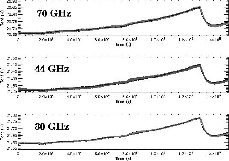
The most relevant instabilities were a 0.5 K peak-to-peak 24-hour fluctuation in the back-end temperature and a 200 mK drift in the reference load temperature caused by a leakage in the gas gap thermal switch that was refilled during the last part of the acquisition (see Fig. 5).

The effect of the reference load temperature variation was clearly identified in the differential radiometric output (see Fig. 6) and removed from the radiometer data before differencing. The effect of the back-end temperature was removed by correlating the radiometric output with temperature sensor measurements.
5.2.3 White noise sensitivity and noise effective bandwidth
There are four sources of the white noise that determines the final sensitivity: (i) the input sky signal; (ii) the RF part of the receiver (active components and resistive losses); (iii) the back-end electronics after the detector diode55 5 The additional noise introduced by the analog electronics is generally negligible compared to the intrisic noise of the receiver, and its impact was further mitigated by the variable gain stage after the diode.; and (iv) signal quantisation performed in the digital processing unit.
Signal quantisation can increase significantly the noise level if , where represents the quantisation step and the noise level before quantisation. Previous optimisation studies (Maris et al. 2003) have shown that a quantisation ratio is enough to satisfy telemetry requirements without significantly increasing the noise level. This has been verified during calibration tests using the so-called “calibration channel”, i.e., a data channel containing about 15 minutes per day of unquantised data from each detector. The use of the calibration channel allowed a comparison between the white noise level before and after quantisation and compression for each detector. Table 9 summarises these results and shows that digital quantisation caused an increase in the signal white noise less than 1%.
The white noise effective bandwidth calculated according to Eq. (4) is reported in Fig. 7. Our results indicate that the noise effective bandwidth is smaller than the requirement by 20%, 50%, and 10% at 30, 44, and 70 GHz, respectively. Non-idealities in the in-band response (ripples) causing bandwidth narrowing are discussed in Zonca et al. (2009).

It is useful to extrapolate these results to the expected in-flight sensitivity with the instrument at the nominal temperature of 20 K and observing a sky signal of K in thermodynamic temperature. This estimate has been performed in two different ways. The first uses measured noise effective bandwidths and noise temperatures in the radiometer equation, Eq. (3). The second starts from measured uncalibrated noise, which is then calibrated in temperature units, corrected for the different focal plane temperature in test conditions, and extrapolated to K input using the radiometeric response equation, Eq (2). The details of the extrapolation are given in Appendix D.
Table 5 gives the sensitivity per radiometer estimated according to the two procedures. The sensitivity per radiometer has been obtained using a weighted noise average from the two detectors of each radiometer (see Appendix E). Because radiometers LFI18M-0 and LFI24M-0 were not working during the tests, we have estimated the sensitivity per frequency channel considering the white noise sensitivity of LFI24M-0 (that was later repaired) measured during receiver-level tests while for LFI18M-0 (that was later replaced with a spare unit) we have assumed the same sensitivity of LFI18S-1. Further details about white noise sensitivity of individual detectors are reported in Meinhold et al. (2009).
| From uncalib. noise | ||
|---|---|---|
| M-0 | S-1 | |
| 70 GHz | ||
| LFI18 | 468 | 468 |
| LFI19 | 546 | 522 |
| LFI20 | 574 | 593 |
| LFI21 | 424 | 530 |
| LFI22 | 454 | 463 |
| LFI23 | 502 | 635 |
| 44 GHz | ||
| LFI24 | 372 | 447 |
| LFI25 | 501 | 492 |
| LFI26 | 398 | 392 |
| 30 GHz | ||
| LFI27 | 241 | 288 |
| LFI28 | 315 | 251 |
| From radiom. equation | ||
|---|---|---|
| M-0 | S-1 | |
| 70 GHz | ||
| LFI18 | 450 | 450 |
| LFI19 | 482 | 466 |
| LFI20 | 498 | 511 |
| LFI21 | 381 | 496 |
| LFI22 | 428 | 410 |
| LFI23 | 453 | 419 |
| 44 GHz | ||
| LFI24 | 404 | 407 |
| LFI25 | 451 | 462 |
| LFI26 | 455 | 428 |
| 30 GHz | ||
| LFI27 | 311 | 320 |
| LFI28 | 305 | 268 |
The sensitivity per frequency channel estimated according the two procedures and compared with the LFI requirement is shown in Table 6.
| Meas. noise | Rad. eq. | Req. | |
|---|---|---|---|
| 70 GHz | 146 | 130 | 105 |
| 44 GHz | 174 | 177 | 113 |
| 30 GHz | 135 | 149 | 116 |
5.2.4 1/ noise parameters
The noise properties of the LFI differenced data have been better determined during instrument-level than receiver-level tests for two reasons: (i) the test performed in this phase has been the longest in all the test campaign, and (ii) because of the better temperature stability, especially compared to the 70 GHz receivers cryofacility (Villa et al. 2009).
best fit with two 1/ components. Being a second-order correction we limit, in this paper, to results obtained with the simple model that Results, summarised in Table 7, show very good noise stability of the LFI receivers, almost all with a knee frequency well below the required 50 mHz.
| (mHz) | ||||
| M-00 | M-01 | S-10 | S-11 | |
| 70 GHz | ||||
| LFI18 | 61 | 59 | ||
| LFI19 | 25 | 32 | 27 | 37 |
| LFI20 | 21 | 19 | 23 | 28 |
| LFI21 | 28 | 30 | 41 | 38 |
| LFI22 | 46 | 39 | 41 | 76 |
| LFI23 | 30 | 31 | 58 | 75 |
| 44 GHz | ||||
| LFI24 | 39 | 46 | ||
| LFI25 | 31 | 31 | 21 | 30 |
| LFI26 | 61 | 61 | 61 | 14 |
| 30 GHz | ||||
| LFI27 | 30 | 30 | 27 | 26 |
| LFI28 | 37 | 31 | 37 | 39 |
| slope | ||||
| M-00 | M-01 | S-10 | S-11 | |
| 70 GHz | ||||
| LFI18 | 1.12 | 1.12 | ||
| LFI19 | 1.27 | 1.22 | 1.11 | 1.02 |
| LFI20 | 1.47 | 1.64 | 1.27 | 1.24 |
| LFI21 | 1.48 | 1.61 | 1.15 | 1.17 |
| LFI22 | 1.18 | 1.26 | 1.19 | 1.01 |
| LFI23 | 1.11 | 1.19 | 1.15 | 1.12 |
| 44 GHz | ||||
| LFI24 | 1.06 | 1.11 | ||
| LFI25 | 1.07 | 1.03 | 1.10 | 1.00 |
| LFI26 | 1.01 | 1.01 | 1.05 | 1.55 |
| 30 GHz | ||||
| LFI27 | 1.06 | 1.13 | 1.25 | 1.13 |
| LFI28 | 0.94 | 0.93 | 1.07 | 1.06 |
5.2.5 Spurious frequency spikes
During the FM test campaign we found unwanted frequency spikes in the radiometeric data at frequencies of the order of few hertz. The source of the problem was recognised to be in the backend data acquisition electronics box, where unexpected crosstalk between the circuits handling housekeeping and radiometric data affected the radiometer voltage output downstream of the detector diode.
This is shown clearly in Fig. 8, which shows spectra of unswitched data acquired from the 70 GHz detector LFI18S-10 with the housekeeping data acquisition activated and deactivated.
(a)
(b)
(c)
(d)
Because the disturbance is added to receiver signal at the end of the radiometric chain it acts as a common mode effect on both the sky and reference load data so that its effect in differenced data is reduced by several orders of magnitude bringing it well below the radiometer noise level.
Further analysis of these spikes has shown that the disturbance is synchronized in time. By binning the data synchronously we obtain a template of the disturbance, which allows its removal in time-domain (Meinhold et al. 2009). The feasibility of this approach has been proven with data acquired during the full satellite test campaign in Liege, Belgium during July and August, 2008.
Therefore, because the only way to eliminate the disturbance in hardware would be to operate the instrument without any housekeeping information, our baseline approach is that, if necessary, the residual effect will be removed from the data in time domain after measuring the disturbance shape from the flight data.
5.3 Radiometric suceptibility to front-end temperature instabilities
Thermal fluctuations in the receivers result in gain changes in the amplifiers and noise changes in the (slightly emissive) passive components (horns, OMTs, waveguides). These changes mimic the effect of changes in sky emission, expecially at fluctuation frequencies near the satellite spin frequency. The most important source of temperature fluctuations for LFI is the sorption cooler (Bhandari et al. 2004; Wade et al. 2000).
For small temperature fluctuations in the focal plane the radiometric response is linear (Seiffert et al. 2002; Terenzi et al. 2009c), so the spurious antenna temperature fluctuation in the differential receiver output can be written as:
| (5) |
Transfer function can be estimated analytically from the differential power output given in Eq. (1):
| (6) |
The analytical form of (Terenzi et al. 2009c, discussed in detail in) depends primarily on the front-end amplifier susceptibility parameters, and as well as on other instrument and boundary condition parameters such as the insertion loss of passive components and the sky input temperature.
If we consider the systematic error budget in Bersanelli et al. (2009), it is possible to derive a requirement for the radiometric transfer function, , in order to maintain the final peak-to-peak error per pixel K (see Appendix F). During instrument-level calibration activities dedicated tests were run to estimate and compare it with theoretical estimates and similar tests performed on individual receivers.
5.3.1 Experimental setup
During this test the focal plane temperature was varied in steps between between 27 and 34 K. The sky and reference load temperatures were K and K. The reference load temperature showed a non-negligible coupling with the focal plane temperature (as shown in Fig 9) so that the effect of this variation had to be removed from the data before calculating the thermal transfer function.

Although the test lasted more than 24 hours, it was difficult to reach a clean steady state plateau after each step because of the large thermal mass of the instrument. Furthermore, for some detectors the bias tuning was not yet optimised, so that only data from a subset of detectors could be compared with similar measurements performed at receiver-level.
In Fig. 10 we summarise our results by comparing predicted and measured transfer functions for the tested detectors. Predicted transfer functions have been calculated using the list of parameters provided in Appendix G, derived from receiver-level tests. In the same figure we also plot the thermal susceptibility requirement rescaled at the experimental test conditions with a scale factor given by the ratio
| (7) |
where has been calculated using Eq. (5) in ground and flight conditions from sky, reference-load and focal plane temperatures.
Fig. 10 shows that transfer functions measured during instrument-level tests are compliant with scientific requirements and reflect theoretical predictions, with the exception of LFI22 and LFI23, which were more susceptible to front-end temperature fluctuations than expected. In general, results from the instrument test campaign confirm design expectations, and suggest that the level of temperature instabilities in the focal plane will not represent a significant source of systematic errors in the final scientific products. This has been further verified during satellite thermal-vacuum tests conducted with the flight model sorption cooler (see Sect. 6.4).


6 Comparison with satellite level test results
The final cryogenic ground test campaign was conducted at the Centre Spatiale de Liège (CSL) with the LFI and the HFI integrated on board Planck. To reproduce flight temperature conditions, the satellite was enclosed in an outer cryochamber cooled to liquid nitrogen temperatures, and surrounded an inner thermal shield at 20 K. An ECCOSORB load cooled to 4.5 K was placed between the secondary mirror and the feed horns to simulate the cold sky. For the first time, the LFI focal plane was cooled to 20 K by the sorption cooler, and the reference loads were cooled to 4 K by the 4 K cooler.
During the CSL tests we verified instrument functionality, tuned front-end biases and back-end electronics, and assessed scientific performance in the closest conditions to flight attainable on the ground. Front-end bias tuning made use of the ability of the 4 K cooler system to provide several different stable temperatures to the reference loads in the range 24 K down to the nominal 4 K (Cuttaia et al. 2009).
A detailed description of satellite-level tests is outside the scope of this paper; here we will focus on the comparison of the main performance parameters measured during instrument and satellite tests, and show that despite differences in test conditions the overall behaviour was reproduced.
6.1 White noise sensitivity
Calibrated white noise sensitivities were determined during satellite-level tests by exploiting a mK variation of the sky load temperature caused by the periodic helium refills of the chamber. This variation allowed us to estimate the photometric calibration constant by correlating the differenced voltage datastream from each detector with the sky load temperature (in antenna temperature units).
To extrapolate the calibrated sensitivity from the 4.5 K input temperature in the test to flight conditions we calculated the ratio:
| (8) |
using the noise temperature found from the non-linear model fit from the receiver-level test campaign (Villa et al. 2009). This ratio ranges from a minimum of 0.96 to a maximum of 0.98. Exact values for each detector are not reported here for simplicity.
In Fig. 11 we summarise graphically the in-flight sensitivity estimates from the three tests. In the following plots the sensitivity values are provided with error bars, with the following meanings:
- •
error bars in sensitivities estimated from satellite-level data represent the statistical error in the calibration constants calculated from the various temperature jumps and propagated through the sensitivity formulas. They represent genuine statistical uncertainties;
- •
error bars in sensitivities estimated from receiver and instrument level tests data represent the uncertainty coming from the calculation performed according to the two different methods described in Sect. 5.2.3 and Appendix D. In this case error bars do not have specific statistical significance, but nevertheless provide an indication of uncertainties in the estimate.
Fig. 11 shows that the in-flight sensitivity lies between the requirement and twice the goal levels for the 30 and 70 GHz receivers, and at about twice the goal for the 44 GHz receivers. The agreement between values extrapolated from the three test campaigns is very good, apart from two noticeable outliers, LFI21S-1 and LFI24M-0, which showed a higher noise level during satellite level tests. Investigation showed that this anomaly was due to incorrect bias voltages on the front-end devices during the test.
After a thorough bias tuning activity conducted during in flight calibration (Cuttaia et al. 2009, see) a new bias configuration was found that normalised the white noise sensitivity of these two receivers, as expected. A full description of the in-flight calibration results and scientific performance will be given in a forthcoming dedicated paper.


6.2 Noise stability
Receiver noise stability during satellite-level tests was determined from stable data acquisitions lasting several hours with the instruments in their tuned and nominal conditions. Fig. 12 summarises knee frequencies measured at instrument and satellite levels compared with the 50 mHz requirement, and shows that the noise stability of all channels is within requirements, with the single marginal exception of LFI23S-11. The slope ranged from a minimum of 0.8 to a maximum of 1.7.
There was a substantial improvement in noise stability during satellite-level tests compared to instrument-level tests, in some cases with a reduction in knee frequency of more than a factor of 2. This can partly be explained by the almost perfect signal input balance achieved in the CSL cryo-facility (much less than 1 K compared to the 3 K obtained in the instrument cryo-facility). Some of the improvement was also expected because of the much better thermal stability of the CSL facility. In particular fluctuations of the sky and reference loads in CSL were about two order of magnitudes less than those in the instrument facility (see Table 3). Because the highly balanced input achieved in CSL will not be reproduced in flight we expect that the flight knee frequencies will be slightly higher (although similar) compared to those measured in CSL.


6.3 Isolation
Isolation (see Eq. (11)) was measured during the satellite tests by changing the reference load temperature by 3.5 K. Fig. 13 compares isolation measured during receiver- and satellite-level tests. Several channels exceed the dB requirement; a few are marginally below. One channel, LFI21S-1, showed poor isolation of only dB. This result is consis with the high value of the calibrated white noise measured for this channel (see Sect. 6.1), supporting the hypothesis of non-optimal biasing of that channel.


6.4 Thermal susceptibility
As mentioned in Sect. 4.3, the most important source of temperature fluctuations in the LFI focal plane is the sorption cooler. The satellite-level test provided the first opportunity to measure the performance of the full Planck thermal system. Fuctuations at the interface between the sorption cooler and the LFI were measured to be about 100 mK peak-to-peak. Using methods described in (Mennella et al. 2002), we calculate that the effect of these fluctuations will be less than 1 K per pixel in the maps, in line with the scientific requirements outlined in Bersanelli et al. (2009).
7 Conclusions
The LFI was integrated and tested in thermo-vacuum conditions at the Thales Alenia Space Italia laboratories, located in Vimodrone (Milano), during the summer of 2006. The test goals were a wide characterisation and calibration of the instrument, ranging from functionality to scientific performance assessment.
The LFI was fully functional, apart from two failed components in LFI18M-0 and LFI24M-0 that have been fixed (one replaced and the other repaired) after the cryogenic test campaign, recovering full functionality.
Measured instrument parameters are consistent with measurements performed on indivudual receivers. In particular, the LFI shows excellent stability and rejection of instrumental systematic effects. Although the very ambitious sensitivity goals have not been fully met, the measured performance makes LFI the most sensitive instrument of its kind, a factor of 2 to 3 better than WMAP66 6 Calculated on the final resolution element per unit integration time at the same frequencies. In particular at 70 GHz, near the minimum of the foreground emission for both temperature and polarisation anisotropy, the combination of sensitivity and angular resolution of LFI will provide a clean reconstruction of the temperature power spectrum up to (Mandolesi et al. 2009).
After the instrument test campaign, the LFI was integrated with the HFI and the satellite. Between June and August 2008, Planck was tested at the Centre Spatiale de Liège in flight-representative, thermo-vacuum conditions, and showed to be fully functional.
Planck was launched on May 14th from the Guyane Space Centre in Kourou and has reached its observation point, L2. In-flight testing and calibration is underway, and will provide the final instrument tuning and scientific performance assessment. After 17 years, Planck is nearly ready to start recording the first light in the Universe.
Acknowledgements.
The Planck-LFI project is developed by an Interntional Consortium lead by Italy and involving Canada, Finland, Germany, Norway, Spain, Switzerland, UK, USA. The Italian contribution to Planck is supported by the Italian Space Agency (ASI). The work in this paper has been supported by in the framework of the ASI-E2 phase of the Planck contract. The US Planck Project is supported by the NASA Science Mission Directorate. In Finland, the Planck LFI 70 GHz work was supported by the Finnish Funding Agency for Technology and Innovation (Tekes).| Rec. ID | Param. | M-00 | M-01 | S-10 | S-11 |
| LFI18 | (V/K) | 0.026 | 0.022 | ||
| (K) | 37.4 | 40.5 | |||
| LFI19 | (V/K) | 0.020 | 0.021 | 0.016 | 0.018 |
| (K) | 39.8 | 38.7 | 37.5 | 40.0 | |
| LFI20 | (V/K) | 0.019 | 0.018 | 0.025 | 0.025 |
| (K) | 42.3 | 42.2 | 43.9 | 43.0 | |
| LFI21 | (V/K) | 0.025 | 0.023 | 0.016 | 0.014 |
| (K) | 31.9 | 34.6 | 43.3 | 45.9 | |
| LFI22 | (V/K) | 0.011 | 0.012 | 0.014 | 0.016 |
| (K) | 40.5 | 38.9 | 40.8 | 43.5 | |
| LFI23 | (V/K) | 0.025 | 0.029 | 0.014 | 0.007 |
| (K) | 40.6 | 39.2 | 50.3 | 54.2 | |
| 1.43 | 1.43 | ||||
| LFI24 | (V/K) | 0.005 | 0.005 | ||
| (K) | 19.7 | 19.9 | |||
| 1.21 | 1.16 | 0.79 | 1.00 | ||
| LFI25 | (V/K) | 0.008 | 0.008 | 0.007 | 0.007 |
| (K) | 19.7 | 19.7 | 20.5 | 20.2 | |
| 1.07 | 1.40 | 0.93 | 1.21 | ||
| LFI26 | (V/K) | 0.005 | 0.006 | 0.007 | 0.007 |
| (K) | 20.2 | 19.1 | 18.5 | 18.1 | |
| 0.12 | 0.12 | 0.12 | 0.14 | ||
| LFI27 | (V/K) | 0.074 | 0.081 | 0.070 | 0.058 |
| (K) | 13.3 | 13.1 | 14.3 | 13.7 | |
| 0.19 | 0.16 | 0.19 | 0.19 | ||
| LFI28 | (V/K) | 0.076 | 0.103 | 0.071 | 0.061 |
| (K) | 11.7 | 11.3 | 10.9 | 10.8 |
| M-00 | M-01 | S-10 | S-11 | |||||||||
| 70 GHz | ||||||||||||
| LFI18 | 38.93 | 39.22 | 0.74% | 31.07 | 31.39 | 1.02% | ||||||
| LFI19 | 33.50 | 33.68 | 0.55% | 34.00 | 34.13 | 0.39% | 25.68 | 25.85 | 0.63% | 27.48 | 27.67 | 0.71% |
| LFI20 | 31.08 | 31.17 | 0.31% | 31.20 | 31.37 | 0.54% | 44.77 | 45.14 | 0.83% | 41.95 | 42.23 | 0.67% |
| LFI21 | 33.77 | 33.94 | 0.51% | 32.27 | 32.39 | 0.35% | 26.50 | 26.67 | 0.62% | 25.63 | 25.86 | 0.87% |
| LFI22 | 17.03 | 17.15 | 0.67% | 19.29 | 19.41 | 0.61% | 20.99 | 21.05 | 0.28% | 23.94 | 24.06 | 0.49% |
| LFI23 | 37.84 | 38.01 | 0.44% | 41.00 | 41.25 | 0.61% | 23.76 | 24.01 | 1.04% | 12.15 | 12.19 | 0.36% |
| 44 GHz | ||||||||||||
| LFI24 | 5.95 | 5.97 | 0.25% | 5.32 | 5.35 | 0.45% | ||||||
| LFI25 | 7.50 | 7.54 | 0.50% | 7.53 | 7.55 | 0.30% | 9.34 | 9.37 | 0.35% | 6.93 | 6.96 | 0.43% |
| LFI26 | 6.04 | 6.06 | 0.32% | 6.18 | 6.20 | 0.31% | 8.81 | 8.84 | 0.28% | |||
| 30 GHz | ||||||||||||
| LFI27 | 62.34 | 62.67 | 0.52% | 65.62 | 65.97 | 0.53% | 56.19 | 56.40 | 0.37% | 52.48 | 52.59 | 0.22% |
| LFI28 | 52.96 | 53.27 | 0.59% | 68.34 | 68.58 | 0.34% | 46.77 | 46.94 | 0.35% | 44.15 | 44.24 | 0.20% |
Appendix A LFI receiver and channel naming convention
The various receivers are labelled LFI18 to LFI28, as shown in Fig. 14. The radiometers connectd to the two OMT arms are labelled M-0 (“main” OMT arm) and S-1 (“side” OMT arm), while the two output detectors from each radiometer are be labelled as 0 and 1. Therefore LFI18S-10, for example, refers to detector 0 of the side arm of receiver LFI18, and LFI24M-01 refers to detector 1 of the main arm of receiver LFI24.

Appendix B Receiver isolation: definition, scientific requirements and measurements
B.1 Definition and requirement.
In Sect. 2 it is shown that the output of the LFI pseudo-correlation receivers is a sequence of sky and reference load signals alternating at twice the phase switch frequency. If the pseudo-correlator is not ideal, the separation after the second hybrid is not perfect and a certain level of mixing between the two signals will be present in the output. Typical limitations on isolation are (i) imperfect hybrid phase matching, (ii) front-end gain amplitude mismatch, and (iii) mismatch in the insertion loss in the two switch states (Seiffert et al. 2002).
A more general relationship representing the receiver power output can be written as:
| (9) | |||||
where the parameters represents the degree of mixing or, in other words, deviation from ideal isolation.
Let us now imagine the receiver scanning the sky and therefore measuring a variation in the sky signal given by the CMB, . If we define and develop Eq. (9) in series up to the first order in we see that the differential power output is proportional to:
| (10) |
where , which provides a useful relationship to estimate the requirement on the isolation, given an acceptable level of .
If we assume 10% (corresponding to ) as the maximum acceptable loss in the CMB signal due to imperfect isolation and consider typical values for the LFI receivers ( K and ranging from 10 to 30 K), we find equivalent to dB, which corresponds to the requirement for LFI receivers.
B.2 Measurement.
If and are the voltage output variations induced by , then it is easy to see from Eq. (9) (with the approximation ) that:
| (11) |
If the reference load temperature is not perfectly stable but varies by an amount during the measurement, this can be corrected at first order if we know the photometric constant . In this case Eq. (11) becomes:
| (12) |
Measuring the isolation accurately, however, is generally difficult and requires a very stable environment. In fact, any change in caused by other systematic fluctuations (e.g., temperature fluctuations, noise fluctuations) will impact the isolation measurement causing an over- or under-estimation depending on the sign of the effect.
To estimate the accuracy in our isolation measurements, we have first calculated the uncertainty caused by a systematic error in the reference load voltage output, . If we substitute in Eq. (12) with and develop at first order in , we obtain
| (13) |
where we indicate with the isolation given by Eq. (12).
We estimated in our measurement conditions. Because the three temperature steps were implemented in about one day we have evaluated the total power signal stability on this timescale from a long-duration acquisition in which the instrument was left running undisturbed for about two days. For each detector datastream we have first removed spurious thermal fluctuations by correlation analysis with temperature sensor data then we calculated the peak-to-peak variation in the reference load datastream.
Appendix C Calculation of noise effective bandwidth
The well-known radiometer equation applied to the output of a single diode in the Planck LFI receivers links the white noise sensitivity to sky and noise temperatures and the receiver bandwidth. It reads (Seiffert et al. 2002):
| (14) |
In the case of linear response, i.e. if (where represents the photometric calibration constant) we can write Eq. (14) in its most useful uncalibrated form:
| (15) |
which is commonly used to estimate the receiver bandwidth, , from a simple measurement of the receiver DC output and white noise level, i.e.:
| (16) |
If the response is linear and if the noise is purely radiometric (i.e. all the additive noise from back end electronics is negligible and if there are no non-thermal noise inputs from the source) then is equivalent to the receiver bandwidth, i.e.
| (17) |
Conversely, if the receiver output is compressed, from Eq. (2) we have that:
| (18) |
| (19) | |||||
which shows that is an overestimate of the “optical” bandwidth unless the non linearity parameter is very small.
Appendix D White noise sensitivity calibration and extrapolation to flight conditions
In this appendix we detail the calculation needed to convert the uncalibrated white noise sensitivity measured on the ground to the expected calibrated sensitivity in flight conditions. The calculation starts from the general radiometric output model in Eq. (2), which can be written in the following form:
| (20) |
Our starting point is the the raw datum, that is a couple of uncalibrated white noise levels for the two detectors in a radiometer measured with the sky load at a temperature and the front end unit at physical temperature .
From the measured uncalibrated white noise level in Volt s1/2, we want to derive a calibrated white noise level extrapolated to input temperature equal to and with the front end unit at a temperature of . This is done in three steps:
- 1.
extrapolation to nominal front-end unit temperature;
- 2.
extrapolation to nominal input sky temperature;
- 3.
calibration in units of K s1/2.
In the following sections we will describe in detail the calculations underlying each step.
D.1 Step 1—extrapolate uncalibrated noise to nominal front end unit temperature
This is a non-trivial step to be performed if we want to consider all the elements in the extrapolation. Here we focus on a zero-order approximation based on the following assumptions:
- 1.
the radiometer noise temperature is dominated by the front-end noise temperature, such that ;
- 2.
we neglect any effect on the noise temperature given by resistive losses of the front-end passive components;
- 3.
we assume the variation of to be linear in .
Under these assumptions the receiver noise temperature at nominal front-end temperature can be written as
| (21) |
where . A similar but slightly different relationship yields for the gain factor . In fact let us consider that , and that we can write , where , i.e.,
| (22) |
From the radiometer equation we have that , from which we can write
| (23) | |||||
where
| (24) |
D.2 Step 2—extrapolate uncalibrated noise to
From this point we will consider quantities (, white noise level, and ) already extrapolated to the nominal front end temperature using Eqs. (21), (22) and (23). Therefore we will now omit the superscript “nom” so that, for example, .
Let us start from the radiometer equation in which, for each detector, the white noise spectral density is given by
| (25) |
Now we want to find a similar relationship for the uncalibrated white noise spectral density linking to . We start from Eq. (18) and calculate the derivative of using Eq. (2) and from Eq. (25). We obtain
| (26) |
where is the bandwidth and is the DC voltage output of the receiver. Considering the two input temperatures and , then the ratio is
| (27) |
If we call the ratio and use Eq. (2) to put in explicit form the ratio of output voltages in Eq. (27) so that , we have
| (28) |
D.3 Step 4—calibrate extrapolated noise
| (29) |
If we call the calibrated noise extrapolated at the sky temperature and consider that, by definition, , the previous equation gives
| (30) |
Appendix E Weighted noise averaging
According to the LFI receiver design the output from each radiometer results from the combination of signals coming from two corresponding detector diodes. Consider two differenced and calibrated datastreams coming from two detectors of a radiometer leg, and . The simplest way to combine the two outputs is to take a straight average, i.e.,
| (31) |
so that the white noise level of the differenced datastream is given by .
This approach, however, is not optimal in cases where the two noise levels are unbalanced, so that the noise of the averaged datastream is dominated by the noisier channel.
An alternative to Eq. (31) is given by a weighting average in which weights are represented by the inverse of the noise levels of the two diode datasteams, i.e.,
| (32) |
or, more generally, in the case where we want to average more than two datastreams together,
| (33) |
For noise-weighted averaging, we choose the weights as so that the white noise of the differenced datastream is given by:
| (34) |
Appendix F Thermal susceptibility scientific requirement
Temperature fluctuations in the LFI focal plane arise primarily from variations in the sorption cooler system driven by the cycles of the six cooler compressors that ‘‘pump’’77 7 The sorption cooler does not use mechanical compressors to generate a high pressure flow, but a process of absorption-desorption of hydrogen into six hydride beds, the “compressors” controlled by a temperature modulation of the beds themselves. the hydrogen in the high pressure piping line to the cooler cold-end. These fluctuations show a frequency spectrum dominated by a period of 1 hour, corresponding to the global warm-up/cool-down cycle of the six compressors.
An active PID temperature stabilisation assembly at the interface between the cooler cold-end and the focal plane achieves stabilities of the order of 80100 mK peak-to-peak with a frequency spectrum dominated by the single compressor frequency ( mHz) and the frequency of the whole assembly ( mHz).
These fluctuations propagate through the focal plane mechanical structure, so that the actual temperature instabilities at the level of the feed-amplifier systems (the term in Eq. (6)) are significantly damped. The LFI thermal model (Tomasi et al. 2009) shows that the fluctuations at the front-end modules are at the level of mK and dominated by the “slowest” components (i.e., those with frequencies Hz).
If we take into account that slow fluctuations in the antenna temperature time stream are further damped by a factor by the scanning strategy and map-making (Mennella et al. 2002), we can easily see from Eq. (6) that a receiver susceptibility is required to maintain the final peak-to-peak error per pixel K.
Appendix G Front-end temperature susceptibility parameters
Temperature susceptibility parameters are summarised in Table 10.
| (dB/K) | ||||
|---|---|---|---|---|
| M-00 | M-01 | S-10 | S-11 | |
| LFI18 | -0.05 | -0.05 | -0.05 | -0.05 |
| LFI19 | -0.05 | -0.04 | -0.02 | -0.03 |
| LFI20 | -0.05 | -0.04 | -0.03 | -0.04 |
| LFI21 | -0.07 | -0.07 | -0.07 | -0.20 |
| LFI22 | -0.21 | -0.15 | -0.18 | -0.13 |
| LFI23 | -0.03 | -0.05 | -0.05 | -0.05 |
| LFI24 | -0.08 | -0.06 | -0.08 | -0.08 |
| LFI25 | -0.02 | -0.02 | -0.04 | -0.05 |
| LFI26 | -0.01 | -0.03 | -0.01 | -0.01 |
| LFI27 | -0.06 | -0.05 | -0.04 | -0.01 |
| LFI28 | -0.03 | -0.07 | -0.14 | -0.13 |
| (K/K) | ||||
|---|---|---|---|---|
| M-00 | M-01 | S-10 | S-11 | |
| LFI18 | 0.47 | 0.49 | 0.38 | 0.42 |
| LFI19 | 0.36 | 0.33 | 0.40 | 0.37 |
| LFI20 | 0.25 | 0.23 | 0.30 | 0.25 |
| LFI21 | 0.15 | 0.15 | 0.18 | 0.30 |
| LFI22 | 0.10 | 0.10 | 0.10 | 0.10 |
| LFI23 | 0.10 | 0.16 | 0.17 | 0.16 |
| LFI24 | 0.40 | 0.41 | 0.10 | 0.43 |
| LFI25 | 0.12 | 0.10 | 0.25 | 0.08 |
| LFI26 | 0.70 | 0.70 | 0.47 | 0.50 |
| LFI27 | 0.81 | 0.45 | 0.58 | 0.34 |
| LFI28 | 0.15 | 0.15 | 0.10 | 0.33 |
References
- Bersanelli et al. (2009) Bersanelli, M., Cappellini, B., Cavaliere, F., et al. 2009, A&A, Accepted
- Bhandari et al. (2004) Bhandari, P., Prina, M., Bowman, R. C., et al. 2004, Cryogenics, 44, 395
- Cuttaia et al. (2009) Cuttaia, F., D’Arcangelo, O., Stringhetti, L., et al. 2009, JINST, 4, T12013
- Davis et al. (2009) Davis, R., Wilkinson, A., Davies, R., et al. 2009, JINST, 4, T12002
- Daywitt (1989) Daywitt, W. 1989, Radiometer equation and analysis of systematic errors for the NIST automated radiometers, Tech. Rep. NIST/TN-1327, NIST
- Dupac & Tauber (2005) Dupac, X. & Tauber, J. 2005, A&A, 430, 363
- Mandolesi et al. (2009) Mandolesi, N., Aja, B., Artal, E., et al. 2009, A&A, Accepted
- Maris et al. (2003) Maris, M., Maino, D., Burigana, C., et al. 2003, Accepted for publication in A&A, astro-ph/0304089
- Martin et al. (2004) Martin, P., Riti, J.-B., & de Chambure, D. 2004, in ESA Special Publication, Vol. 554, 5th International Conference on Space Optics, ed. B. Warmbein, 323–331
- Meinhold et al. (2009) Meinhold, P., Leonardi, R., Artal, E., et al. 2009, JINST, 4, T12009
- Mennella et al. (2002) Mennella, A., Bersanelli, M., Burigana, C., et al. 2002, A&A, 384, 736
- Mennella et al. (2003) Mennella, A., Bersanelli, M., Seiffert, M., et al. 2003, A&A, 410, 1089
- Mennella et al. (2009) Mennella, A., Villa, F., Terenzi, L., et al. 2009, JINST, 4, T12011
- Seiffert et al. (2002) Seiffert, M., Mennella, A., Burigana, C., et al. 2002, A&A, 391, 1185
- Tauber (2009) Tauber, J. 2009, A&A, Submitted
- Terenzi et al. (2009a) Terenzi, L., Bersanelli, M., Battaglia, P., et al. 2009a, JINST, Submitted
- Terenzi et al. (2009b) Terenzi, L., Lapolla, M., Laaninen, M., et al. 2009b, JINST, 4, T12015
- Terenzi et al. (2009c) Terenzi, L., Salmon, M., Colin, A., et al. 2009c, JINST, 4, T12012
- Tomasi et al. (2009) Tomasi, M., Cappellini, B., Gregorio, A., et al. 2009, JINST, Submitted
- Valenziano et al. (2009) Valenziano, L., De Rosa, A., Cuttaia, F., et al. 2009, JINST, 4, T12005
- Varis et al. (2009) Varis, J., Hughes, N., Laaninen, M., et al. 2009, JINST, 4, T12001
- Villa et al. (2002) Villa, F., Bersanelli, M., Burigana, C., et al. 2002, in American Institute of Physics Conference Series, Vol. 616, Experimental Cosmology at Millimetre Wavelengths, ed. M. de Petris & M. Gervasi, 224–228
- Villa et al. (2009) Villa, F., Bersanelli, M., Cappellini, B., et al. 2009, A&A, Submitted
- Wade et al. (2000) Wade, L., Bhandari, P., Bowman, J. R., et al. 2000, in Advances in Cryogenic Engineering, ed. et al. Kluwer Academic/Plenum New York Q-S. Shu, Vol. 45A, 499–506
- Zonca et al. (2009) Zonca, A., Franceschet, C., Battaglia, P., Villa, F., & Mennella, A. 2009, JINST, 4, T12010