On the BICM CapacityThanks: Research supported by the Swedish Research Council, Sweden under grant #2006-5599. This work has been presented in part at the International Wireless Communications and Mobile Computing Conference IWCMC 2009, Leipzig, Germany, June 2009, and the IEEE Information Theory Workshop ITW 2009, Taormina, Italy, Oct. 2009.

Hereafter we use lowercase letters $x$ to denote a scalar, boldface letters $\boldsymbol{x}$ to denote a row vector of scalars, and underlined symbols $\underline{\boldsymbol{x}}$ to denote a sequence. Blackboard bold letters $\mathbb{X}$ represent matrices and $x_{i,j}$ represents the entry of $\mathbb{X}$ at row $i$, column $j$, where all the indices start at zero. The transpose of $\mathbb{X}$ is denoted by $\mathbb{X}^{\mathrm{T}}$, $\mathop{\mathrm{trace}\left(\mathbb{X}\right)}\nolimits$ is the trace of $\mathbb{X}$, and $\|\mathbb{X}\|^{2}$ is $\mathop{\mathrm{trace}\left(\mathbb{X}^{\mathrm{T}}\mathbb{X}\right)}\nolimits$.

We denote random variables by capital letters $Y$, probabilities by $\Pr\{\cdot\}$, the probability mass function (pmf) of the random vector $\boldsymbol{Y}$ by $P_{\boldsymbol{Y}}(\boldsymbol{y})$, and the probability density function (pdf) of the random vector $\boldsymbol{Y}$ by $p_{\boldsymbol{Y}}(\boldsymbol{y})$. The joint pdf of the random vectors $\boldsymbol{X}$ and $\boldsymbol{Y}$ is denoted by $p_{\boldsymbol{X},\boldsymbol{Y}}(\boldsymbol{x},\boldsymbol{y})$, and the conditional pdf of $\boldsymbol{Y}$ conditioned on $\boldsymbol{X}=\boldsymbol{x}$ is denoted by $p_{\boldsymbol{Y}|\boldsymbol{X}=\boldsymbol{x}}(\boldsymbol{y})$. The same notation applies to joint and conditional pmfs, i.e., $P_{\boldsymbol{X},\boldsymbol{Y}}(\boldsymbol{x},\boldsymbol{y})$ and $P_{\boldsymbol{Y}|\boldsymbol{X}=\boldsymbol{x}}(\boldsymbol{y})$. The expectation of an arbitrary function $f(\boldsymbol{X},\boldsymbol{Y})$ over the joint pdf of $\boldsymbol{X}$ and $\boldsymbol{Y}$ is denoted by $\mathds{E}_{\boldsymbol{X},\boldsymbol{Y}}[f(\boldsymbol{X},\boldsymbol{Y})]$, the expectation over the conditional pdf $p_{\boldsymbol{Y}|\boldsymbol{X}=\boldsymbol{x}}(\boldsymbol{y})$ is denoted by $\mathds{E}_{\boldsymbol{Y}|\boldsymbol{X}=\boldsymbol{x}}[f(\boldsymbol{X},\boldsymbol{Y})]$, and $\mathop{\mathrm{cov}\left(\boldsymbol{X}\right)}\nolimits$ is the covariance matrix of the random vector $\boldsymbol{X}$.

We denote the base-2 representation of the integer $0\leq i\leq M-1$, where $M=2^{m}$, by the vector $\boldsymbol{b}(i)=[b_{m-1}(i),b_{m-2}(i),\ldots,b_{0}(i)]$, where $b_{m-1}(i)$ is the most significant bit of $i$ and $b_{0}(i)$ the least significant. To facilitate some of the developments in this paper, we also define the ordered direct product as

where $\boldsymbol{c}_{qi+j}=[\boldsymbol{a}_{i},\boldsymbol{b}_{j}]$ for $i=0,\ldots,p-1$ and $j=0,\ldots,q-1$. The ordered direct product in (1) is analogous to the Cartesian product except that it operates on vectors/matrices instead of sets.

A binary labeling $\mathbb{L}$ of order $m\geq 1$ is defined using an $M\times m$ matrix where each row corresponds to one of the $M$ length-$m$ distinct binary codewords, $\mathbb{L}=[\boldsymbol{c}_{0}^{\mathrm{T}},\ldots,\boldsymbol{c}_{M-1}^{\mathrm{T}}]^{\mathrm{T}}$, where $\boldsymbol{c}_{i}=[c_{i,0},c_{i,1},\ldots,c_{i,m-1}]\in\{0,1\}^{m}$.

In order to recursively define some particular binary labelings, we first define expansions, repetitions, and reflections of binary labelings. To expand a labeling $\mathbb{L}_{m}=[\boldsymbol{c}_{0}^{\mathrm{T}},\ldots,\boldsymbol{c}_{M-1}^{\mathrm{T}}]^{\mathrm{T}}$ into a labeling $\mathbb{L}_{m+1}$, we repeat each binary codeword once to obtain a new matrix $[\boldsymbol{c}_{0}^{\mathrm{T}},\boldsymbol{c}_{0}^{\mathrm{T}},\ldots,\boldsymbol{c}_{M-1}^{\mathrm{T}},\boldsymbol{c}_{M-1}^{\mathrm{T}}]^{\mathrm{T}}$, and then we obtain $\mathbb{L}_{m+1}$ by appending one extra column $[0,1,1,0,0,1,1,0,\ldots,0,1,1,0]^{\mathrm{T}}$ of length $2M$ [27]. To generate a labeling $\mathbb{L}_{m+1}$ from a labeling $\mathbb{L}_{m}=[\boldsymbol{c}_{0}^{\mathrm{T}},\ldots,\boldsymbol{c}_{M-1}^{\mathrm{T}}]^{\mathrm{T}}$ by repetition, we repeat the labeling $\mathbb{L}_{m}$ once to obtain a new matrix $[\boldsymbol{c}_{0}^{\mathrm{T}},\ldots,\boldsymbol{c}_{M-1}^{\mathrm{T}},\boldsymbol{c}_{0}^{\mathrm{T}},\ldots,\boldsymbol{c}_{M-1}^{\mathrm{T}}]^{\mathrm{T}}$, and we add an extra column from the left, consisting of $M$ zeros followed by $M$ ones. Finally, to generate a labeling $\mathbb{L}_{m+1}$ from a labeling $\mathbb{L}_{m}=[\boldsymbol{c}_{0}^{\mathrm{T}},\ldots,\boldsymbol{c}_{M-1}^{\mathrm{T}}]^{\mathrm{T}}$ by reflection, we join $\mathbb{L}_{m}$ and a reversed version of $\mathbb{L}_{m}$ to obtain a new matrix $[\boldsymbol{c}_{0}^{\mathrm{T}},\ldots,\boldsymbol{c}_{M-1}^{\mathrm{T}},\boldsymbol{c}_{M-1}^{\mathrm{T}},\ldots,\boldsymbol{c}_{0}^{\mathrm{T}}]^{\mathrm{T}}$, and we add an extra column from the left, consisting of $M$ zeros followed by $M$ ones [27].

In this paper we are particularly interested in the binary reflected Gray code (BRGC)[28, 29], the natural binary code (NBC), and the folded binary code (FBC) [30]. The FBC was analyzed in [30] for uncoded transmission and here we will, to our knowledge for the first time, consider it for coded transmission. In Sec. III-D and Sec. V-C it is shown to yield a higher capacity than other labelings under some conditions. We also introduce a new binary labeling denoted binary semi-Gray code (BSGC). These binary labelings are generated as follows:

• •

  The BRGC $\mathbb{G}_{m}$ of order $m\geq 1$ is generated by $m-1$ recursive expansions of the trivial labeling $\mathbb{L}_{1}=[0,1]^{\mathrm{T}}$, or, alternatively, by $m-1$ recursive reflections of $\mathbb{L}_{1}$.

• •

  The NBC $\mathbb{N}_{m}$ of order $m\geq 1$ is defined as the codewords $\boldsymbol{c}_{i}$ that are the base-2 representations of the integers $i=0,\ldots,M-1$, i.e., $\mathbb{N}_{m}=[\boldsymbol{b}(0)^{\mathrm{T}},\ldots,\boldsymbol{b}(M-1)^{\mathrm{T}}]^{\mathrm{T}}$. Alternatively, $\mathbb{N}_{m}$ can be generated by $m-1$ recursive repetitions of the trivial labeling $\mathbb{L}_{1}$, or as $m-1$ ordered direct products of $\mathbb{L}_{1}$ with itself.

• •

  The BSGC $\mathbb{S}_{m}$ of order $m\geq 3$ is generated by replacing the first column of $\mathbb{G}_{m}$ by the modulo-2 sum of the first and last columns.

• •

  The FBC $\mathbb{F}_{m}$ of order $m\geq 2$ is generated by one reflection of $\mathbb{N}_{m-1}$.

For any labeling matrix $\mathbb{L}=[\boldsymbol{c}_{0}^{\mathrm{T}},\ldots,\boldsymbol{c}_{M-1}^{\mathrm{T}}]^{\mathrm{T}}$, where $\boldsymbol{c}_{i}=[c_{i,0},c_{i,1},\ldots,c_{i,m-1}]\in\{0,1\}^{m}$, we define a modified labeling matrix $\mathbb{Q}=\mathbb{Q}(\mathbb{L})$ which is obtained by reversing the order of the columns and applying the mapping $(0\rightarrow 1,1\rightarrow-1)$, i.e.,

with $i=0,\ldots,M-1$ and $k=0,\ldots,m-1$.

Throughout this paper, we use $\mathcal{X}$ to represent the set of symbols used for transmission. Each element of $\mathcal{X}$ is an $N$-dimensional symbol $\boldsymbol{x}_{i}$, $i=0,\ldots,M-1$, where $|\mathcal{X}|=M=2^{m}$ and $\mathcal{X}\subset\mathds{R}^{N}$. We define the input alphabet using an $M\times m$ matrix $\mathbb{X}=[\boldsymbol{x}_{0}^{\mathrm{T}},\ldots,\boldsymbol{x}_{M-1}^{\mathrm{T}}]^{\mathrm{T}}$ which contains all the elements of $\mathcal{X}$.

For practical reasons, we are interested in well structured input alphabets. An $M$-PAM input alphabet is defined by the column vector $\mathbb{X}_{\mathrm{PAM}}$ where $x_{i,1}=-(M-2i-1)$ with $i=0,\ldots,M-1$. An $M$-PSK input alphabet is the matrix $\mathbb{X}_{\mathrm{PSK}}$ where $\boldsymbol{x}_{i}=\left[\cos\frac{(2i+1)\pi}{M},\sin\frac{(2i+1)\pi}{M}\right]$ with $i=0,1,\ldots,M-1$. Finally, a rectangular $(M^{\prime}\times M^{\prime\prime})$-QAM input alphabet is the $M^{\prime}M^{\prime\prime}\times 2$ matrix $\mathbb{X}_{\mathrm{QAM}}=\mathbb{X}^{\prime}_{\mathrm{PAM}}\otimes\mathbb{X}^{\prime\prime}_{\mathrm{PAM}}$, where $\mathbb{X}^{\prime}_{\mathrm{PAM}}$ and $\mathbb{X}^{\prime\prime}_{\mathrm{PAM}}$ are vectors of length $M^{\prime}$ and $M^{\prime\prime}$, respectively.

For a given input alphabet $\mathbb{X}$, the input distribution of the symbols is denoted by the pmf $P_{\boldsymbol{X}}(\boldsymbol{x})$, which represents the probabilities of transmitting the symbols $\boldsymbol{x}$, i.e., $\Pr\{\boldsymbol{X}=\boldsymbol{x}\}$. We define the matrix $\mathbb{P}$ as an ordered list containing the probabilities of the symbols, i.e., $\mathbb{P}\triangleq[P_{\boldsymbol{X}}(\boldsymbol{x}_{0}),\ldots,P_{\boldsymbol{X}}(\boldsymbol{x}_{M-1})]^{\mathrm{T}}$. We use $\mathbb{U}_{M}\triangleq[1/M,\ldots,1/M]^{\mathrm{T}}$ to denote the discrete uniform input distribution.

We define a constellation as the list of matrices $\Omega\triangleq[\mathbb{X},\mathbb{L},\mathbb{P}]$, i.e., an input alphabet using a given labeling and input distribution. Finally, for a given pair $[\mathbb{X},\mathbb{L}]$, we denote with $\mathcal{I}_{k,u}\subset\{0,\ldots,M-1\}$ the set of indexes of the symbols with a binary label $u\in\{0,1\}$ at bit position $k\in\{0,\ldots,m-1\}$, i.e., $\mathcal{I}_{k,u}\triangleq\{i\in\{0,\ldots,M-1\}:c_{i,k}=u\}$.

In this paper, we analyze coded modulation schemes (CM) as the one shown in Fig. 1. Each of the $K$ possible messages is represented by the binary vector $\boldsymbol{w}\in\{0,1\}^{k_{c}}$, where $k_{c}=\log_{2}{K}$. The transmitter maps each message to a sequence $\underline{\boldsymbol{x}}=[\boldsymbol{x}(0)^{\mathrm{T}},\ldots,\boldsymbol{x}(N_{\mathrm{s}}-1)^{\mathrm{T}}]^{\mathrm{T}}\in\mathcal{X}^{N_{\mathrm{s}}}$, which corresponds to $N_{\mathrm{s}}$ $N$-dimensional symbols ($N_{\mathrm{s}}$ channel uses²² 2 A “channel use” corresponds to the transmission of one $N$-dimensional symbol, i.e., it can be considered as a “vectorial channel use”.). The code $\mathbbmss{C}$ is a subset of $\mathcal{X}^{N_{\mathrm{s}}}$ such that $|\mathbbmss{C}|=K$, which is used for transmission. The transmitter is then defined as a one-to-one function that assigns each information message $\boldsymbol{w}$ to one of the $K$ possible sequences $\underline{\boldsymbol{x}}\in\mathbbmss{C}$. The code rate in information bits per coded bits is then given by $R=\dfrac{k_{c}}{mN_{\mathrm{s}}}$ or, equivalently, $R_{\mathrm{c}}=\dfrac{k_{c}}{N_{\mathrm{s}}}$ information bits per channel use (information bits per symbol, or information bits per $N$ real dimensions). At the receiver’s side, based on the channel observations, a maximum likelihood sequence receiver generates an estimate of the information bits $\boldsymbol{\hat{w}}$ selecting the most likely transmitted message.

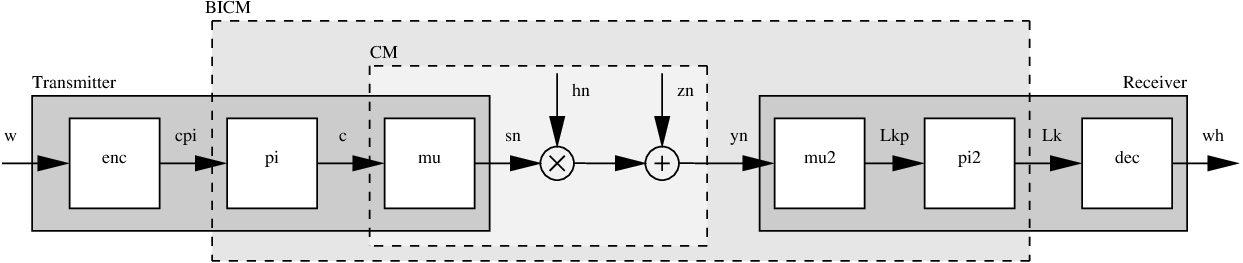
We consider transmissions over a discrete-time memoryless fast fading channel

where the operator $\circ$ denotes the so-called Schur product (element-wise product) between two vectors, $\boldsymbol{X}(t)$, $\boldsymbol{H}(t)$, $\boldsymbol{Y}(t)$, and $\boldsymbol{Z}(t)$ are the underlying random vectors for $\boldsymbol{x}(t)$, $\boldsymbol{h}(t)$, $\boldsymbol{y}(t)$, and $\boldsymbol{z}(t)$ respectively, with $t=0,\ldots,N_{\mathrm{s}}-1$ being the discrete time index, and $\boldsymbol{Z}(t)$ is a Gaussian noise with zero mean and variance $N_{0}/2$ in each dimension. The channel is represented by the $N$-dimensional vector $\boldsymbol{H}(t)$, and it contains real fading coefficients $H_{i}$ which are assumed to be random variables, possibly dependent, with same pdf $p_{H}(h)$. We assume that $\boldsymbol{H}(t)$ and $N_{0}$ are perfectly known at the receiver or can be perfectly estimated. Since the channel is memoryless, from now on we drop the index $t$.

The conditional transition pdf of the channel in (3) is given by

We assume that both $\boldsymbol{H}$ and $\boldsymbol{X}$ have finite and nonzero second moments, that $\boldsymbol{X}$, $\boldsymbol{H}$, and $\boldsymbol{Z}$ are mutually independent, and that there exists a constant $\omega>0$ such that for all sufficiently large $\Delta>0$ the vector $\boldsymbol{H}$ satisfies

This condition will be used in the proof of Theorem 7 in Sec. IV-C.

Each transmitted symbol conveys $R_{\mathrm{c}}$ information bits and thus, the relation between the average symbol energy $E_{\mathrm{s}}\triangleq\mathds{E}_{\boldsymbol{X}}[\|\boldsymbol{X}\|^{2}]$ and the average information bit energy $E_{\mathrm{b}}$ is given by $E_{\mathrm{s}}=R_{\mathrm{c}}E_{\mathrm{b}}$. We define the average signal-to-noise ratio (SNR) as

The AWGN channel is obtained as a special case of (3) by taking $\boldsymbol{H}$ as the all-one vector. Another particular case is obtained when $H_{0}=H_{1}=\ldots=H_{N-1}=A$, which particularizes to the Rayleigh fading channel when $A=\sqrt{A_{1}^{2}+A_{2}^{2}}$ and $A_{1},A_{2}$ are independent zero-mean Gaussian random variables. In this case, the instantaneous SNR defined by $\mathds{E}_{\boldsymbol{X}}[\|\boldsymbol{H}\circ\boldsymbol{X}\|^{2}]/N_{0}=A^{2}E_{\mathrm{s}}/N_{0}$ follows a chi-square distribution with one degree of freedom (an exponential distribution). Similarly, the Nakagami-$m$ fading channel is obtained when $A$ follows a Nakagami-$m$ distribution. It can be shown that the condition (5) is fulfilled in all the cases above.

In a BICM system [12, 13], the transmitter in Fig. 1 is realized using a serial concatenation of a binary encoder of rate $R=R_{\mathrm{c}}/m$, a bit level interleaver, and a memoryless mapper $\Phi$. The mapper $\Phi$ is defined as a one-to-one mapping rule that maps the length-$m$ binary random vector $\boldsymbol{C}=[C_{0},\ldots,C_{m-1}]$ to one symbol $\boldsymbol{X}$, i.e., $\Phi:\{0,1\}^{m}\rightarrow\mathcal{X}$. At the receiver’s side, the demapper computes soft information on the coded bits, which are then deinterleaved and passed to the channel decoder. The a posteriori L-values for the $k$th bit in the symbol and for a given fading realization are given by

where to pass from (8) to (9), the so-called max-log [31] approximation was used.

The max-log metric in (9) (already proposed in[12, 13]) is suboptimal; however, it is very popular in practical implementations because of its low complexity, e.g., in the 3rd generation partnership project (3GPP) working groups [32]. It is also known that when Gray-labeled constellations are used, the use of this simplification results in a negligible impact on the receiver’s performance [33, Fig. 9] [34, Fig. 6]. The max-log approximation also allows BICM implementations which do not require the knowledge of $N_{0}$, for example, when a Viterbi decoder is used, or when the demapper passes hard decisions to the decoder. Moreover, the use of the max-log approximation transforms the nonlinear relation $l_{k}(\boldsymbol{y})$ in (8) into a piecewise linear relation. This has been used to develop expressions for the pdf of the L-values in (9) using arbitrary input alphabets [35] (based on an algorithmic approach), closed-form expressions for QAM input alphabets labeled by the BRGC for the AWGN channel [36, 37], and for fading channels [38]. Recently, closed-form approximations for the pdf of the L-values in (9) for arbitrary input alphabets and binary labeling in fading channels have been presented [39].

The Hadamard transform (HT) is a discrete, linear, orthogonal transform, like for example the Fourier transform, but its coefficients take values in $\pm 1$ only. Among the different applications that the HT has, one that is often overlooked is as an analysis tool for binary labelings [40, 41]. The HT is defined by means of an $M\times M$ matrix, the Hadamard matrix, which is defined recursively as follows when $M$ is a power of two [25, pp. 53–54].

In the following, we will drop the index, letting $\mathbb{H}$ represent a Hadamard matrix of any size $M=2^{m}$. Hadamard matrices have the following appealing properties.

It can be shown [42, Sec. 1.1][43, Sec. III] that the elements of a Hadamard matrix are $h_{i,j}=\prod_{k=0}^{m-1}(-1)^{b_{k}(i)b_{k}(j)}$, from which we observe for future use that for all $i=0,\ldots,M-1$ and $l=0,\ldots,m-1$,

where $b_{l}(i)$ is the $l$th bit of the base-2 representation of the integer $i$.

At this point it is interesting to note the close relation between the columns of the matrix $\mathbb{Q}(\mathbb{N}_{3})$ in Example 1 and the columns $2^{l}$ of $\mathbb{H}_{8}$ in (2) for $l=0,1,2$. Its generalization is given by the following lemma, whose proof follows immediately from (2), the definition of the NBC in Sec. II-B, and (19).

The HT operates on a vector of length $M=2^{m}$, for any integer $m$, or in a more general case, on a matrix with $M=2^{m}$ rows. The transform of a matrix $\mathbb{X}$ is denoted $\tilde{\mathbb{X}}$ and has the same dimensions as $\mathbb{X}$. It is defined as

and the inverse transform is $\mathbb{X}=\mathbb{H}\tilde{\mathbb{X}}$. Equivalently,

where from (18) we have that $h_{j,i}=h_{i,j}$, and where we have introduced the row vectors $\boldsymbol{x}_{i}$ and $\tilde{\boldsymbol{x}}_{j}$ such that

Because of (19), the first element of the transform is simply $\tilde{\boldsymbol{x}}_{0}=\frac{1}{M}\sum_{i=0}^{M-1}\boldsymbol{x}_{i}$.

Finally, using $\sum_{j=0}^{M-1}\|\tilde{\boldsymbol{x}}_{j}\|^{2}=\mathrm{trace}\bigl(\tilde{\mathbb{X}}^{\mathrm{T}}\tilde{\mathbb{X}}\bigr)$, (21), and (18), we note that a variant of Parseval’s theorem holds:

In this subsection, we assume the use of a continuous input alphabet, i.e., $\mathcal{X}=\mathds{R}^{N}$, which upperbounds the performance of finite input alphabets.

The average mutual information (AMI) in bits³³ 3 Throughout this paper all the AMIs are given in bits. per channel use between the random vectors $\boldsymbol{X}$ and $\boldsymbol{Y}$ when the channel is perfectly known at the receiver is defined as

where we use $\boldsymbol{X}$ as the index of $I_{\boldsymbol{X}}(\boldsymbol{X};\boldsymbol{Y})$ to emphasize the fact that the AMI depends on the input PDF $p_{\boldsymbol{X}}(\boldsymbol{x})$. For an arbitrary channel parameter $\boldsymbol{H}$, the AMI in (24) can be expressed as⁴⁴ 4 We note that the AMI with perfect channel state information is usually denoted by $I_{\boldsymbol{X}}(\boldsymbol{X};\boldsymbol{Y}|\boldsymbol{H})$, however, and for notation simplicity, we use $I_{\boldsymbol{X}}(\boldsymbol{X};\boldsymbol{Y})$.

where $p_{\boldsymbol{Y}|\boldsymbol{X}=\boldsymbol{x},\boldsymbol{H}=\boldsymbol{h}}(\boldsymbol{y})$ is given by (4).

The channel capacity of a continuous-input continuous-output memoryless channel is defined as the maximum AMI between its input and output [44, Ch. 4][45, eq. (3)]

where the maximization is over all possible input distributions. The capacity in (27) has units of [bit/channel use] (or equivalently [bit/symbol]), and it is an upper bound on the number of bits per symbol that can be reliably transmitted through the channel, where a symbol consists of $N$ real dimensions. Shannon’s channel coding theorem states that it is not possible to transmit information reliably above this fundamental limit, i.e.,

The AWGN capacity, denoted by $\mathsf{C}^{\mathrm{AW}}\left(\mathsf{SNR}\right)$, is defined as the channel capacity of the AWGN channel (obtained from (3) using $\boldsymbol{H}(t)=\boldsymbol{1}$), and it is given by [44, Sec. 9.4]

This capacity is attained when $\boldsymbol{X}$ are i.i.d. zero-mean Gaussian random variables with variance $E_{\mathrm{s}}/N$ in each dimension and it follows from the fact that the noise is independent in each dimension, and thus, the transmission of $\boldsymbol{X}$ can be considered as a transmission through $N$ parallel independent Gaussian channels.

We define the conditional AMI for discrete input alphabets as the AMI between $\boldsymbol{X}$ and $\boldsymbol{Y}$ conditioned on the outcome of a third random variable $U$, i.e.,

which is valid for any random $\boldsymbol{H}$.

The CM capacity is defined as the AMI between $\boldsymbol{X}$ and $\boldsymbol{Y}$ for a given constellation $\Omega$, i.e.,

where to pass from (32) to (33), we used the fact that the mapping rule between $\boldsymbol{C}$ and $\boldsymbol{X}$ is one-to-one. To pass from (33) to (34) we have used the chain rule of mutual information [44, Sec. 2.5], where $I_{\boldsymbol{X}}(C_{k};\boldsymbol{Y}|C_{0},\ldots,C_{k-1})$ represents a bit level AMI which represents the maximum rate that can be used at the $(k+1)$th bit position, given a perfect knowledge of the previous $k$ bits.

The CM capacity in (32) corresponds to the capacity of the memoryless “CM channel” in Fig. 1 for a given constellation $\Omega$. We note that different binary labelings will produce different values of $I_{\boldsymbol{X}}(C_{k};\boldsymbol{Y}|C_{0},\ldots,C_{k-1})$ in (34); however, the overall sum will remain constant, i.e., the CM capacity does not depend on the binary labeling. We use the name “CM capacity” for $\mathsf{I}^{\mathrm{CM}}_{\Omega}\left(\mathsf{SNR}\right)$ in (32) following the standard terminology⁵⁵ 5 Sometimes, this is also called joint capacity [26], or (constellation) constrained capacity [46, 47]. used in the literature (cf. [13, 21, 48, 23, 49]), although we recognize the misusage of the word capacity since no optimization over the input distribution is performed (cf. (27)). Moreover, it is also possible to optimize the input alphabet in order to obtain an increase in the AMI (so-called signal shaping [50]). Nevertheless, throughout this paper we will refer to the AMI for a given $\Omega$ in (32) as the CM capacity.

In this paper we are interested in optimal constellations, and therefore, we define the maximum CM capacity as

As mentioned before, the CM capacity does not depend on the binary labeling, i.e., it does not depend on how the mapping rule $\Phi$ is implemented, and therefore, in (36) we only show two optimization parameters: the input alphabet and the input distribution.

The CM capacity in (32) (for a given constellation $\Omega$) is an upper bound on the number of bits per symbol that can be reliably transmitted using for example TCM [9] or MLC with multistage decoding (MLC-MSD)[10, 51]. MLC-MSD is in fact a direct application of the summation in (34), i.e., $m$ parallel encoders are used, each of them having a rate $R_{k}=I_{\boldsymbol{X}}(C_{k};\boldsymbol{Y}|C_{0},\ldots,C_{k-1})$. At the receiver’s side, the first bit level is decoded and the decisions are passed to the second decoder, which then passes the decisions to the third decoder, and so on. Other design rules can also be applied in MLC, cf. [51]. The maximum CM capacity $\mathsf{C}^{\mathrm{CM}}\left(\mathsf{SNR}\right)$ in (36) represents an upper bound on the number of bits per symbol that can be reliably transmitted using a fully optimized system, i.e., a system where for each SNR value $\mathsf{SNR}$, the input alphabet and the input distribution are selected in order to maximize the CM capacity $\mathsf{I}^{\mathrm{CM}}_{\Omega}\left(\mathsf{SNR}\right)$.

It is commonly assumed that the sequence generated by the binary encoder in Fig. 1 is infinitely long and symmetric, and also that the interleaver ($\pi$) operates over this infinite sequence, simply permuting it in a random way. Under these standard assumptions, it follows that the input symbol distribution will be always $\mathbb{P}=\mathbb{U}_{M}$. Since in this paper we are interested in analyzing a more general setup where the input symbol distribution can by modified, we develop a more general model in which we relax the equiprobable input distribution assumption.

Let $C_{k}\in\{0,1\}$ the binary random variable representing the bits at the $k$th modulator’s input, where the pmf $P_{C_{k}}(u)$ represents the probability of transmitting a bit $u$ at bit position $k$. We assume that in general $\sum_{k=0}^{m-1}P_{C_{k}}(0)\neq\sum_{k=0}^{m-1}P_{C_{k}}(1)$, i.e., the coded and interleaved sequence could have more zeros than ones (or vice-versa). Note that since $P_{C_{k}}(u)$ is a pmf, $P_{C_{k}}(0)+P_{C_{k}}(1)=1$.

Let $\boldsymbol{c}_{i}=[c_{i,0},\ldots,c_{i,m-1}]$ be the binary label of the symbol $\boldsymbol{x}_{i}$. We assume that the bits at the input of the modulator are independent, and therefore, the input symbol probabilities are

The independence condition on the coded bits that results in (37) can be obtained if the interleaver block in Fig. 1 completely breaks the temporal correlation of the coded bits. The condition that the coded and interleaved sequence could be asymmetric can be obtained for example by using an encoder with nonuniform outputs, or by a particular puncturing scheme applied to the coded bits. This can be combined with the use of multiple interleavers and multiplexing [52], which would allow $P_{C_{k}}(u)\neq 1/2$. Examples of how to construct a BICM scheme where nonuniform input symbol distributions are obtained include the “shaping encoder” of [53, 54] and the nonuniform signaling scheme based on a Huffman code of [55].

For future use, we also define the conditional input symbol probabilities, conditioned on the $k$th bit being $u$, as

where $\mathcal{I}_{i,k}$ is defined in Sec. II-C.

The “BICM channel” in Fig. 1 was introduced in [56] and it is what separates the encoder and decoder in a BICM system. The BICM capacity is then defined as the capacity of the BICM channel. Using the definitions in Sec. III-C and the equivalent channel model in [13, Fig. 6], which replaces the BICM channel by $m$ parallel binary-input continuous-output channels, the BICM capacity for a given constellation $\Omega$ is defined as

where (42) follows from (41), (38), and the fact that the value of $C_{k}$ does not affect the conditional channel transition probability, i.e., $p_{\boldsymbol{Y}|\boldsymbol{X}=\boldsymbol{x},\boldsymbol{H}=\boldsymbol{h},C_{k}=u}(\boldsymbol{y})=p_{\boldsymbol{Y}|\boldsymbol{X}=\boldsymbol{x},\boldsymbol{H}=\boldsymbol{h}}(\boldsymbol{y})$. The BICM capacity in (42) is a general expression that depends on all the constellation parameters $\Omega$. This can be numerically implemented using Gauss–Hermite quadratures, or alternatively, by using a one-dimensional integration based on the pdf of the L-values developed in [35, 37, 38, 39].

The AMIs $I_{C_{k}}(C_{k};\boldsymbol{Y})$ in (39) are, in contrast to the ones in (36), not conditioned on the previous bit values. Because of this, and unlike the CM capacity, the binary labeling strongly affects the BICM capacity $\mathsf{I}^{\mathrm{BI}}_{\Omega}\left(\mathsf{SNR}\right)$ in (39). Note that the BICM capacity is equivalent to the capacity achieved by MLC with (suboptimal) parallel decoding of the individual bit levels, because in BICM, the bits are treated as independent [51]. The differences are that BICM uses only one encoder, and that in BICM the equivalent channels are not used in parallel, but time multiplexed. Again, following the standard terminology⁶⁶ 6 It is also called parallel decoding capacity in [26], or receiver constrained capacity in [46]. used in the literature (cf. [13, 21, 48, 23, 49]), we use the name “BICM capacity” even though no optimization over the input distribution is performed.

If all the bits at the input of the modulator are equally likely, i.e., $P_{C_{k}}(u)=1/2$ for $k=0,\ldots,m-1$ and $u\in\{0,1\}$, we obtain from (37) $P_{\boldsymbol{X}}(\boldsymbol{x})=1/M$. Under these constraints, and assuming an AWGN channel ($\boldsymbol{H}=\boldsymbol{1}$), the BICM capacity in (42) is given by

where the constellation is $\Omega=[\mathbb{X},\mathbb{L},\mathbb{U}_{M}]$. This expression coincides with the “standard” BICM capacity formula (cf. [57, Sec. 3.2.1], [13, eq. (15)], [48, eq. (11)]).

One relevant question here is what is the optimum labeling from a capacity maximization point of view. Once this question is answered, approaching the fundamental limit will depend only on a good design of the channel encoder/decoder. Caire et al. conjectured the optimality of the BRGC, which, as the next example shows, is not correct at all SNR. This was first disproved in [24] for PAM input alphabets based on an exhaustive search of binary labelings up to $M=8$.

Formally, $E_{\mathrm{b}}/N_{0}$ is bounded from below by $f(R_{\mathrm{c}})$, where

This function always exists, because the capacity⁷⁷ 7 From now on we will refer to “capacity” using the notation $\mathsf{C}(\mathsf{SNR})$ in a broad sense. $\mathsf{C}(\mathsf{SNR})$ can be the AWGN capacity $\mathsf{C}^{\mathrm{AW}}(\mathsf{SNR})$ in (29), the CM capacity $\mathsf{I}_{\Omega}^{\mathrm{CM}}(\mathsf{SNR})$ in (32), or the BICM capacity $\mathsf{I}_{\Omega}^{\mathrm{BI}}(\mathsf{SNR})$ in (39). $\mathsf{C}(\mathsf{SNR})$ is a strictly increasing⁸⁸ 8 This can be proved using the relation between the AMI and the minimum mean square error (MMSE) presented in [59], i.e., that the derivative of the AMI with respect to $\mathsf{SNR}$ is proportional to the MMSE for any $\mathsf{SNR}$. Since the MMSE is a strictly decreasing function of $\mathsf{SNR}$, the AMI is a strictly increasing function of $\mathsf{SNR}$. function of $\mathsf{SNR}$ and thus invertible, while in contrast $f(R_{\mathrm{c}})$ is in general not monotone. This is the reason why a given $E_{\mathrm{b}}/N_{0}$ for some labelings maps to more than one capacity value, as shown in [21]. The phenomenon can be understood by considering the function $\mathsf{I}^{\mathrm{BI}}_{\Omega}(\mathsf{SNR})$ in a linear $\mathsf{SNR}$ scale, instead of logarithmic as in Fig. 2 (a). If plotted, the function would pass through the origin for all labelings. Furthermore, any straight line through the origin represents a constant $\mathds{E}_{H}[H^{2}]E_{\mathrm{b}}/N_{0}$ by (6), where the slope is determined by the value of $\mathds{E}_{H}[H^{2}]E_{\mathrm{b}}/N_{0}$. Such a line cannot intersect $\mathsf{I}^{\mathrm{BI}}_{\Omega}(\mathsf{SNR})$ more than once for $\mathsf{SNR}>0$, if $\mathsf{I}^{\mathrm{BI}}_{\Omega}(\mathsf{SNR})$ is concave. This is the case for the BRGC, NBC, and FBC, and therefore the function $R_{\mathrm{c}}=f^{-1}(\mathds{E}_{H}[H^{2}]E_{\mathrm{b}}/N_{0})$ exists, as illustrated for in Fig. 2 (b). However, for some labelings such as the BSGC (and many others shown in [49, Fig. 3.5]), $\mathsf{I}^{\mathrm{BI}}_{\Omega}(\mathsf{SNR})$ is not concave and $f(R_{\mathrm{c}})$ is not invertible. This phenomenon has also been observed for linear precoding for BICM with iterative demapping and decoding [60, Fig. 3], punctured turbo codes [61, Fig. 3], and incoherent $M$-ary PSK [62, Figs. 2 and 5] and frequency-shift keying channels [63, Figs. 1 and 6].

References

- [1] H. Nyquist, “Certain factors affecting telegraph speed,” Bell System Technical Journal, pp. 324–346, Apr. 1924.
- [2] ——, “Certain topics in telegraph transmission theory,” Trans. of the A.I.E.E., vol. 47, no. 2, pp. 617–644, Apr. 1928.
- [3] R. V. L. Hartley, “Transmission of information,” Bell System Technical Journal, pp. 535–563, July 1928.
- [4] C. E. Shannon, “A mathematical theory of communications,” Bell System Technical Journal, vol. 27, pp. 379–423 and 623–656, July and Oct. 1948.
- [5] ——, “Communication in the presence of noise,” Proceedings of the IRE, vol. 37, no. 1, pp. 10–21, Jan. 1949.
- [6] J. R. Pierce, “The early days of information theory,” IEEE Trans. Inf. Theory, vol. IT-19, no. 1, pp. 3–8, Jan. 1973, (Invited Paper).
- [7] J. L. Massey, “Coding and modulation in digital communications,” in International Zurich Seminar on Digital Communications, Zurich, Switzerland, Mar. 1974.
- [8] G. Ungerboeck and I. Csajka, “On improving data-link performance by increasing channel alphabet and introducing sequence decoding,” in International Symposium on Information Theory (ISIT), Ronneby, Sweden, June 1976.
- [9] G. Ungerboeck, “Channel coding with multilevel/phase signals,” IEEE Trans. Inf. Theory, vol. 28, no. 1, pp. 55–67, Jan. 1982.
- [10] H. Imai and S. Hirakawa, “A new multilevel coding method using error-correcting codes,” IEEE Trans. Inf. Theory, vol. IT-23, no. 3, pp. 371–377, May 1977.
- [11] ——, “Correction to ‘A new multilevel coding method using error-correcting codes’,” IEEE Trans. Inf. Theory, vol. IT-23, no. 6, p. 784, Nov. 1977.
- [12] E. Zehavi, “8-PSK trellis codes for a Rayleigh channel,” IEEE Trans. Commun., vol. 40, no. 3, pp. 873–884, May 1992.
- [13] G. Caire, G. Taricco, and E. Biglieri, “Bit-interleaved coded modulation,” IEEE Trans. Inf. Theory, vol. 44, no. 3, pp. 927–946, May 1998.
- [14] 3GPP, “Universal mobile telecommunications system (UMTS); multiplexing and channel coding (FDD),” 3GPP, Tech. Rep. TS 25.212, V8.5.0 Release 8, Mar. 2009.
- [15] E. Dahlman, S. Parkvall, J. Sköld, and P. Beming, 3G Evolution: HSPA and LTE for Mobile Broadband, 2nd ed. Academic Press, 2008.
- [16] IEEE 802.11, “Part 11: Wireless LAN medium access control (MAC) and physical layer (PHY) specifications: High-speed physical layer in the 5GHz band,” IEEE Std 802.11a-1999(R2003), Tech. Rep., July 1999.
- [17] IEEE 802.11n, “Part 11: Wireless LAN medium access control (MAC) and physical layer (PHY) specifications. Amendment 5: Enhancements for higher throughout,” IEEE Std 802.11n-2009, Tech. Rep., Oct. 2009.
- [18] ETSI, “Digital video broadcasting (DVB); Frame structure channel coding and modulation for a second generation digital terrestrial television broadcasting system (DVB-T2),” ETSI, Tech. Rep. ETSI EN 302 755 V1.1.1 (2009-09), Sep. 2009.
- [19] ——, “Digital video broadcasting (DVB); Second generation framing structure, channel coding and modulation systems for broadcasting, interactive services, news gathering and other broadband satellite applications (DVB-S2),” ETSI, Tech. Rep. ETSI EN 302 307 V1.2.1 (2009-08), Aug. 2009.
- [20] ——, “Digital video broadcasting (DVB); Frame structure channel coding and modulation for a second generation digital transmission system for cable system (DVB-C2),” ETSI, Tech. Rep. ETSI EN 302 769 V1.1.1 (2010-04), Apr. 2010.
- [21] A. Martinez, A. Guillén i Fàbregas, and G. Caire, “Bit-interleaved coded modulation in the wideband regime,” IEEE Trans. Inf. Theory, vol. 54, no. 12, pp. 5447–5455, Dec. 2008.
- [22] A. Alvarado, E. Agrell, A. Guillén i Fàbregas, and A. Martinez, “Corrections to ‘Bit-interleaved coded modulation in the wideband regime’,” IEEE Trans. Inf. Theory, vol. 56, no. 12, p. 6513, Dec. 2010.
- [23] C. Stierstorfer and R. F. H. Fischer, “Asymptotically optimal mappings for BICM with -PAM and -QAM,” IET Electronics Letters, vol. 45, no. 3, pp. 173–174, Jan. 2009.
- [24] ——, “(Gray) Mappings for bit-interleaved coded modulation,” in IEEE Vehicular Technology Conference (VTC-Spring), Dublin, Ireland, Apr. 2007.
- [25] F. J. MacWilliams and N. J. A. Sloane, The Theory of Error-Correcting Codes. Amsterdam, The Netherlands: North-Holland, 1977.
- [26] M. Barsoum, C. Jones, and M. Fitz, “Constellation design via capacity maximization,” in IEEE International Symposium on Information Theory (ISIT), Nice, France, June 2007.
- [27] E. Agrell, J. Lassing, E. G. Ström, and T. Ottosson, “On the optimality of the binary reflected Gray code,” IEEE Trans. Inf. Theory, vol. 50, no. 12, pp. 3170–3182, Dec. 2004.
- [28] F. Gray, “Pulse code communications,” U. S. Patent 2 632 058, Mar. 1953.
- [29] E. Agrell, J. Lassing, E. G. Ström, and T. Ottosson, “Gray coding for multilevel constellations in Gaussian noise,” IEEE Trans. Inf. Theory, vol. 53, no. 1, pp. 224–235, Jan. 2007.
- [30] J. Lassing, E. G. Ström, E. Agrell, and T. Ottosson, “Unequal bit-error protection in coherent -ary PSK,” in IEEE Vehicular Technology Conference (VTC-Fall), Orlando, FL, USA, Oct. 2003.
- [31] A. J. Viterbi, “An intuitive justification and a simplified implementation of the MAP decoder for convolutional codes,” IEEE J. Sel. Areas Commun., vol. 16, no. 2, pp. 260–264, Feb. 1998.
- [32] Ericsson, Motorola, and Nokia, “Link evaluation methods for high speed downlink packet access (HSDPA),” TSG-RAN Working Group 1 Meeting #15, TSGR1#15(00)1093, Tech. Rep., Aug. 2000.
- [33] B. Classon, K. Blankenship, and V. Desai, “Channel coding for 4G systems with adaptive modulation and coding,” IEEE Wireless Commun. Mag., vol. 9, no. 2, pp. 8–13, Apr. 2002.
- [34] A. Alvarado, H. Carrasco, and R. Feick, “On adaptive BICM with finite block-length and simplified metrics calculation,” in IEEE Vehicular Technology Conference (VTC-Fall), Montreal, QC, Canada, Sep. 2006.
- [35] L. Szczecinski, R. Bettancourt, and R. Feick, “Probability density function of reliability metrics in BICM with arbitrary modulation: Closed-form through algorithmic approach,” IEEE Trans. Commun., vol. 56, no. 5, pp. 736–742, May 2008.
- [36] M. Benjillali, L. Szczecinski, and S. Aissa, “Probability density functions of logarithmic likelihood ratios in rectangular QAM,” in Twenty-Third Biennial Symposium on Communications, Kingston, ON, Canada, May 2006.
- [37] A. Alvarado, L. Szczecinski, R. Feick, and L. Ahumada, “Distribution of L-values in Gray-mapped -QAM: Closed-form approximations and applications,” IEEE Trans. Commun., vol. 57, no. 7, pp. 2071–2079, July 2009.
- [38] L. Szczecinski, A. Alvarado, and R. Feick, “Distribution of max-log metrics for QAM-based BICM in fading channels,” IEEE Trans. Commun., vol. 57, no. 9, pp. 2558–2563, Sep. 2009.
- [39] A. Kenarsari-Anhari and L. Lampe, “An analytical approach for performance evaluation of BICM over Nakagami- fading channels,” IEEE Trans. Commun., vol. 58, no. 4, pp. 1090–1101, Apr. 2010.
- [40] P. Knagenhjelm and E. Agrell, “The Hadamard transform—a tool for index assignment,” IEEE Trans. Inf. Theory, vol. 42, no. 4, pp. 1139–1151, July 1996.
- [41] F. A. Khan, E. Agrell, and M. Karlsson, “Electronic dispersion compensation by Hadamard transformation,” in Optical Fiber Conference (OFC), San Diego, CA, USA, Mar. 2010.
- [42] E. E. Sutter, “The fast -transform: a fast computation of cross-correlations with binary -sequences,” SIAM J. Comput., vol. 20, no. 4, pp. 686–694, Aug. 1991.
- [43] W. K. Pratt, J. Kane, and H. C. Andrews, “Hadamard transform image coding,” Proceedings of the IEEE, vol. 57, no. 1, pp. 58–72, Jan. 1969.
- [44] T. Cover and J. Thomas, Elements of Information Theory, 2nd ed. New York, USA: John Wiley & Sons, 2006.
- [45] T. Cover and M. Chiang, “Duality between channel capacity and rate distortion with two-sided state information,” IEEE Trans. Inf. Theory, vol. 48, no. 6, pp. 1629–1638, June 2002.
- [46] F. Schreckenbach, “Iterative decoding of bit-interleaved coded modulation,” Ph.D. dissertation, Technische Universität München, Munich, Germany, 2007, available at http://mediatum2.ub.tum.de/doc/644160/644160.pdf.
- [47] F. Brännström and L. K. Rasmussen, “Classification of unique mappings for 8PSK based on bit-wise distance spectra,” IEEE Trans. Inf. Theory, vol. 55, no. 3, pp. 1131–1145, Mar. 2009.
- [48] A. Martinez, A. Guillén i Fàbregas, and G. Caire, “Bit-interleaved coded modulation revisited: A mismatched decoding perspective,” IEEE Trans. Inf. Theory, vol. 55, no. 6, pp. 2756–2765, June 2009.
- [49] C. Stierstorfer, “A bit-level-based approach to coded multicarrier transmission,” Ph.D. dissertation, Friedrich-Alexander-Universität Erlangen-Nürnberg, Erlangen, Germany, 2009, available at http://www.opus.ub.uni-erlangen.de/opus/volltexte/2009/1395/.
- [50] R. F. H. Fischer, Precoding and Signal Shaping for Digital Transmission. John Wiley & Sons, 2002.
- [51] U. Wachsmann, R. F. H. Fischer, and J. B. Huber, “Multilevel codes: Theoretical concepts and practical design rules,” IEEE Trans. Inf. Theory, vol. 45, no. 5, pp. 1361–1391, July 1999.
- [52] A. Alvarado, E. Agrell, L. Szczecinski, and A. Svensson, “Exploiting UEP in QAM-based BICM: Interleaver and code design,” IEEE Trans. Commun., vol. 58, no. 2, pp. 500–510, Feb. 2010.
- [53] S. Le Goff, B. S. Sharif, and S. A. Jimaa, “Bit-interleaved turbo-coded modulation using shaping coding,” IEEE Commun. Lett., vol. 9, no. 3, pp. 246–248, Mar. 2005.
- [54] S. Le Goff, B. K. Khoo, C. C. Tsimenidis, and B. S. Sharif, “Constellation shaping for bandwidth-efficient turbo-coded modulation with iterative receiver,” IEEE Trans. Wireless Commun., vol. 6, no. 6, pp. 2223–2233, June 2007.
- [55] D. Raphaeli and A. Gurevitz, “Constellation shaping for pragmatic turbo-coded modulation with high spectral efficiency,” IEEE Trans. Commun., vol. 52, no. 3, pp. 341–345, Mar. 2004.
- [56] A. Martinez, A. Guillén i Fàbregas, and G. Caire, “Error probability analysis of bit-interleaved coded modulation,” IEEE Trans. Inf. Theory, vol. 52, no. 1, pp. 262–271, Jan. 2006.
- [57] A. Guillén i Fàbregas, A. Martinez, and G. Caire, “Bit-interleaved coded modulation,” Foundations and Trends in Communications and Information Theory, vol. 5, no. 1–2, pp. 1–153, 2008.
- [58] S. Verdú, “Spectral efficiency in the wideband regime,” IEEE Trans. Inf. Theory, vol. 48, no. 6, pp. 1319–1343, June 2002.
- [59] D. Guo, S. Shamai, and S. Verdú, “Mutual information and minimum mean-square error in Gaussian channels,” IEEE Trans. Inf. Theory, vol. 51, no. 4, pp. 1261–1282, Apr. 2005.
- [60] F. Simoens, H. Wymeersch, and M. Moeneclaey, “Linear precoders for bit-interleaved coded modulation on AWGN channels: Analysis and design criteria,” IEEE Trans. Inf. Theory, vol. 54, no. 1, pp. 87–99, Jan. 2008.
- [61] F. Brännström, L. K. Rasmussen, and A. J. Grant, “Optimal puncturing ratios and energy allocation for multiple parallel concatenated codes,” IEEE Trans. Inf. Theory, vol. 55, no. 5, pp. 2062–2077, May 2009.
- [62] M. Peleg and S. Shamai, “On the capacity of the blockwise incoherent MPSK channel,” IEEE Trans. Commun., vol. 46, no. 5, pp. 603–609, May 1998.
- [63] W. E. Stark, “Capacity and cutoff rate of noncoherent FSK with nonselective Rician fading,” IEEE Trans. Commun., vol. COM-33, no. 11, pp. 1153–1159, Nov. 1985.
- [64] A. Guillén i Fàbregas and A. Martinez, “Bit-interleaved coded modulation with shaping,” in IEEE Information Theory Workshop (ITW), Dublin, Ireland, Aug.–Sep. 2010.
- [65] D. Guo, S. Shamai, and S. Verdú, “Estimation of non-Gaussian random variables in Gaussian noise: Properties of the MMSE,” in IEEE International Symposium on Information Theory (ISIT), Toronto, ON, Canada, July 2008.
- [66] ——, “Estimation in Gaussian noise: Properties of the minimum mean-square error,” IEEE Trans. Inf. Theory, vol. 57, no. 1, Jan. 2011, available at http://arxiv.org/abs/1004.3332.
- [67] D. Zwillinger, Standard Mathematical Tables and Formulae, 31st ed. Boca Raton, FL: CRC Press, 2003.
- [68] C. E. Shannon, “Coding theorems for a discrete source with a fidelity criterion,” in IRE National Convention Record, New York, NY, Mar. 1959, pp. 142–163, vol. 7, pt. 4.
- [69] P. K. Vitthaladevuni and M.-S. Alouini, “A recursive algorithm for the exact BER computation of generalized hierarchical QAM constellations,” IEEE Trans. Inf. Theory, vol. 49, no. 1, pp. 297–307, Jan. 2003.
- [70] M. Morimoto, M. Okada, and S. Komaki, “A hierarchical image transmission system in fading channel,” in IEEE International Conference on Universal Personal Communications (ICUPC), Tokyo, Japan, Oct. 1995, pp. 769–772.
- [71] Md. J. Hossain, M.-S. Alouini, and V. K. Bhargava, “Hierarchical constellation for multi-resolution data transmission over block fading channels,” IEEE Trans. Wireless Commun., vol. 5, no. 4, pp. 849–857, Apr. 2006.
- [72] D. Divsalar and F. Pollara, “On the design of turbo codes,” Jet Propulsion Laboratory, Pasadena, CA, TDA Progr. Rep. 42-123, pp. 99–121, Nov. 1995, available at http://tmo.jpl.nasa.gov/progress_report/42-123/123D.pdf.
- [73] V. V. Prelov and S. Verdú, “Second-order asymptotics of mutual information,” IEEE Trans. Inf. Theory, vol. 50, no. 8, pp. 1567–1580, Aug. 2004.
- [74] I. S. Gradshteyn and I. M. Ryzhik, Tables of Integrals, Series and Products, 6th ed. New York, NY: Academic Press, 1980.