Communication in a Poisson Field of Interferers – Part II: Channel Capacity and Interference Spectrum

We start with the complex baseband characterization of the probe link, obtained in Part I by projecting all signals onto a cosine-sine orthonormal set. Thus, the complex channel output $\mathbf{Z}$ can be written as

where $\mathbf{S}$ is the complex channel input, and $\mathbf{\widetilde{W}}$ is the combined aggregate interference and thermal noise, given by

with $\mathbf{W}\sim\mathcal{N}_{\textrm{c}}(0,N_{0}).$⁴⁴ 4 We use $\mathcal{N}_{\textrm{c}}(0,\sigma^{2})$ to denote a circularly symmetric (CS) complex Gaussian distribution, where the real and imaginary parts are i.i.d. $\mathcal{N}(0,\sigma^{2}/2)$. These are essentially the same baseband equations as those given in Part I, except that the transmitted constellation symbol $a_{0}e^{j\theta_{0}}$ has been replaced by a generic input symbol $\mathbf{S}$, with an arbitrary distribution $f_{\mathbf{S}}(s)$. This emphasizes the fact that to analyze the channel capacity, we need to maximize the mutual information over all possible input distributions $f_{\mathbf{S}}(s)$, and thus cannot restrict $\mathbf{S}$ to belong to a specific constellation, such as $M$-PSK or $M$-QAM. In addition, we impose an average energy constraint on the input symbol by requiring that $\mathbb{E}\{|\mathbf{S}|^{2}\}\leq E_{\mathrm{S}}$.

Considering that the interfering nodes are coded and operating close to capacity, then the signal transmitted by each interferer is Gaussian, such that $\mathbf{X}_{i}\sim\mathcal{N}_{\textrm{c}}(0,2V_{X})$ [13].⁵⁵ 5 Alternatively, we can follow the same approach as in Part I and argue that $\mathbf{X}_{i}\sim\mathcal{N}_{\textrm{c}}(0,2V_{X})$ in a scenario where the interferers employ an arbitrary two-dimensional modulation (this is the Gaussian approximation introduced in [8, Eq. (10)]. In such case, $V_{X}$ is a function of the constellation of the interferers, as shown in [8, Eq. (13)]. The resulting aggregate network interference is thus Gaussian when conditioned on $\mathcal{P}$, and the distribution of $\mathbf{\widetilde{W}}$ in (2) is given by⁶⁶ 6 We use $X\,\mathop{\sim}\limits^{{\scriptscriptstyle|Y}}$ to denote the distribution of $X$ conditional on $Y$.

where

Note that since $A$ in (4) depends on $\mathcal{P}$ (i.e., $\{R_{i}\}_{i=1}^{\infty}$ and $\{G_{i}\}_{i=1}^{\infty}$), it can be seen as a random variable (r.v.) whose value is different for each realization of $\mathcal{P}$. It was shown in Part I that the r.v. $A$ has a skewed stable distribution [14] given by⁷⁷ 7 We use $\mathcal{S}(\alpha,\beta,\gamma)$ to denote a real stable distribution with characteristic exponent $\alpha\in(0,2]$, skewness $\beta\in[-1,1]$, and dispersion $\gamma\in[0,\infty)$. The corresponding characteristic function is $$\phi(w)=\begin{cases}\exp\left[-\gamma|w|^{\alpha}\left(1-j\beta\mathrm{\,sign}(w)\tan\frac{\pi\alpha}{2}\right)\right],&\alpha\neq 1,\\ \exp\left[-\gamma|w|\left(1+j\frac{2}{\pi}\beta\mathrm{\,sign}(w)\ln|w|\right)\right],&\alpha=1.\end{cases}$$

where $b>1$, and $C_{x}$ is defined as

with $\Gamma(x)=\int_{0}^{\infty}t^{x-1}e^{-t}dt$ denoting the gamma function.

Because of the conditioning on $G_{0}$ and $\mathcal{P}$, equations (1)-(4) describe a simple Gaussian channel depicted schematically in Fig. 1. The capacity of this energy-constrained, fast fading channel with receiver CSI can be written as [15]

where $I(\mathbf{S};\mathbf{Z}|\alpha_{0})$ is the conditional mutual information between $\mathbf{S}$ and $\mathbf{Z}$ given $\alpha_{0}$. The optimal input distribution that maximizes the mutual information is therefore $\mathcal{N}_{\mathrm{c}}(0,E_{\mathrm{S}})$. With this input distribution,

in bits per complex symbol, and thus we obtain the capacity of the channel as

in bits per complex symbol, where we have explicitly indicated the conditioning of $C$ on the random interferer positions and shadowing. For a Rayleigh fading channel, $\alpha_{0}^{2}$ is exponentially distributed with mean $1$ and we can further express (7) in terms of the exponential integral function $\textrm{Ei}(x)=-\int_{-x}^{\infty}\frac{e^{-t}}{t}dt$ as

in bits per complex symbol, where

is the received signal-to-interference-plus-noise ratio (SINR), averaged over the fast fading.

In the proposed quasi-static model, the maximum rate of reliable communication for a given realization of $G_{0}$ and $\mathcal{P}$ is given by (8)-(9). Such quantity is a function of the random user positions and shadowing, and is therefore random. Then, with some probability, $G_{0}$ and $\mathcal{P}$ are such that the capacity is below the transmission rate $R$, thus making the channel unusable for communication at that rate with arbitrarily low error probability. The system is said to be in outage, and the capacity outage probability is

or, substituting $(\ref{eq:C-G0-P-Ei})$ into (10),

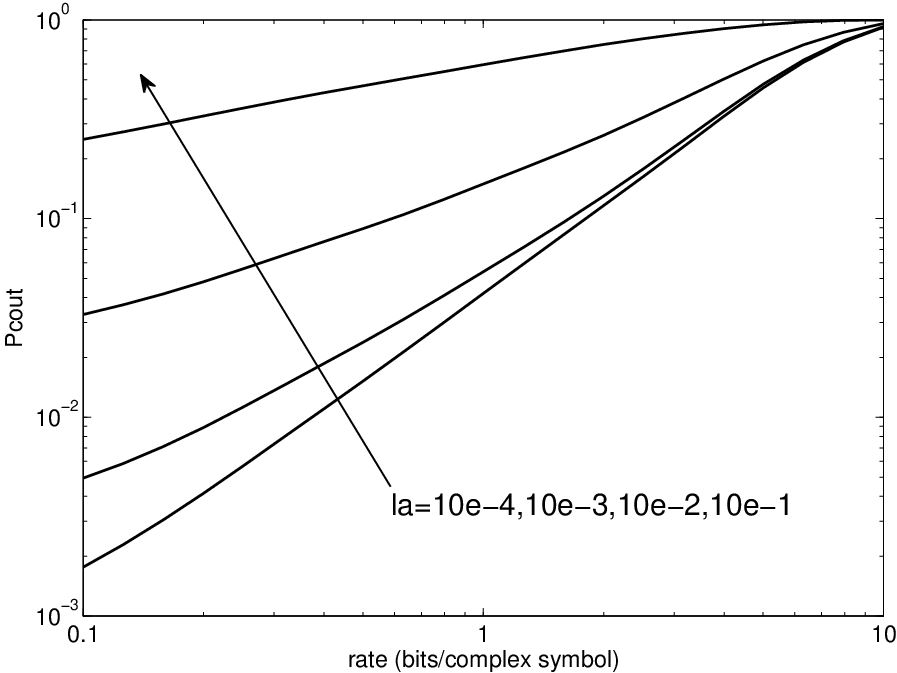
Figures 2 and 3 quantify the capacity outage probability and illustrate its dependence on the various parameters, such as the signal-to-noise ratio $\mathsf{SNR}=E_{\mathrm{S}}/N_{0}$, the interference-to-noise ratio $\mathsf{INR}=E/N_{0}$, and spatial density $\lambda$ of the interferers. For simplicity, we consider a case study where all interfering nodes transmit equiprobable symbols, belonging to a constellation that is symmetric with respect to the origin of the IQ-plane (e.g., $M$-PSK and $M$-QAM). In this particular case, it is shown in [8, Eq. (13)] that $V_{X}=E/3$, and thus (9) reduces to

To evaluate the corresponding $P_{\textrm{out}}^{\textrm{c}}$, we resort to a hybrid approach where we employ the analytical result given in (11)-(12), but perform a Monte Carlo simulation of the stable r.v. $A$ according to [16]. Nevertheless, we emphasize that the expressions derived in this paper completely eliminate the need for simulation of the interferers’ positions and waveforms in the network, in order to obtain the capacity.

The aggregate network emission at the probe receiver can be characterized by the complex baseband random process $\mathbf{Y}(t)$, defined as

where $\mathbf{Y}_{\hskip-1.0pti}(t)$ is the received process associated with each emitting node $i$. The signal $\mathbf{Y}_{\hskip-1.0pti}(t)$ can in turn be expressed for all time $t$ as

where $\mathbf{X}_{i}(t)$ is the complex baseband transmitted signal, and $\mathbf{h}_{i}(t,\tau)$ is time-varying complex baseband impulse response of the multipath channel associated with node $i$. The system model described by (14) is depicted in Fig. 4. It corresponds to a generalization of the model introduced in Part I of this paper, where we considered a two-dimensional modulation and a flat Rayleigh fading channel. Since now we are interested in analyzing the spectral properties of $\mathbf{Y}(t)$, we incorporate in the model a generic transmitted waveform $\mathbf{X}_{i}(t)$, not necessarily associated with a two-dimensional modulation, as well as a generic multipath channel $\mathbf{h}_{i}(t,\tau)$, not necessarily associated with flat Rayleigh fading. Also, since in this section we are only interested in the aggregate emission of the network, we can ignore the existence of the probe link depicted in [8, Fig. 1]. In what follows we carry the analysis in complex baseband, although it can be trivially translated to passband frequencies.

In the remainder of this paper, we consider that the transmitted signal $\mathbf{X}_{i}(t)$ is a wide-sense stationary (WSS) process, such that its autocorrelation function has the form $R_{\mathbf{X}_{i}}(t_{1},t_{2})\triangleq\mathbb{E}\{\mathbf{X}_{i}^{*}(t_{1})\mathbf{X}_{i}(t_{2})\}=R_{\mathbf{X}}(\Delta t)$, where $\Delta t=t_{2}-t_{1}$. We define the PSD of the process $\mathbf{X}_{i}(t)$ as $\mathcal{S}_{\mathbf{X}}(f)\triangleq\mathcal{F}_{\Delta t\rightarrow f}\{R_{\mathbf{X}}(\Delta t)\}$.⁸⁸ 8 We use $\mathcal{F}_{x\rightarrow y}\{\cdot\}$ to denote the Fourier transform operator, where $x$ and $y$ represent the independent variables in the original and transformed domains, respectively. Since different nodes operate independently, the processes $\mathbf{X}_{i}(t)$ are also independent for different $i$, but the underlying second-order statistics are the same (i.e., the autocorrelation function and the PSD of $\mathbf{X}_{i}(t)$ do not depend on $i$). As we will show in the case study of Section IV-C, if $\mathbf{X}_{i}(t)$ is a train of pulses with a uniformly distributed random delay (which models the asynchronism between emitting nodes), then it is a WSS process.

In terms of the multipath channel, we consider a wide-sense stationary uncorrelated scattering (WSSUS) channel [17, 18, 19, 20, 21], so that the autocorrelation function of $\mathbf{h}_{i}(t,\tau)$ can be expressed as

for some function $P_{\mathbf{h}}(\Delta t,\tau)$. Such channel can be represented in the form of a densely-tapped delay line, as a continuum of uncorrelated, randomly-scintillating scatterers having WSS statistics. The functions $\mathbf{h}_{i}(t,\tau)$ are considered to be independent for different nodes $i$, but the underlying second-order statistics are the same (i.e., the autocorrelation function of $\mathbf{h}_{i}(t,\tau)$ does not depend on $i$). WSSUS channels are an important class of practical channels which simultaneously exhibit wide-sense stationarity in the time variable $t$ and uncorrelated scattering in the delay variable $\tau$. They are the simplest non-degenerate channels which exhibit both time and frequency fading, and also serve as a good model for many radio channels.

We now wish to derive the PSD of the aggregate RF emission $\mathbf{Y}(t)$ of the network, and with that purpose we introduce the following theorem.

In the proposed quasi-static scenario, the PSD of the aggregate network emission $\mathcal{S}_{\mathbf{Y}}(f,\mathcal{P})$ is a function of the random node positions and shadowing, $\mathcal{P}$. Then, with some probability, $\mathcal{P}$ is such that the spectrum of the aggregate emission is too high in some frequency band of interest, thus causing an outage in that frequency band. This leads to the concept of spectral outage probability (SOP), which we denote by $P_{\textrm{out}}^{\textrm{s}}(f)$ and generally define as

where $\mathcal{S}_{\mathbf{Y}}(f,\mathcal{P})$ is the random PSD of the aggregate network emission $\mathbf{Y}(t)$, and $m(f)$ is some spectral mask determining the outage (or detection) threshold at the receiver. The SOP is a frequency-dependent quantity and, in the case of slow-varying positions $\mathcal{P}$, is a more insightful metric than the PSD averaged over $\mathcal{P}$. Note that this definition is applicable in general to any emission model: the spectral outage probability $P_{\textrm{out}}^{\textrm{s}}(f)$ represents the probability that the PSD of the aggregate network emission, measured at an arbitrary location in the plane and at a particular frequency $f$, exceeds some predetermined mask.

In commercial applications, the concept of SOP can provide a radically different way to establish spectral regulations. Current regulations and standards (e.g., FCC Part 15 or IEEE 802.11) impose a spectral mask on the PSD at the transmitter, and the type of mask often depends on the environment in which the devices are operated (e.g., indoor or outdoor). The purpose of this mask is to limit RF emissions generated by a terminal, and to protect other services that operate in dedicated bands (e.g., Global Positioning System, public safety, and cellular systems). However, the transmitted PSD is usually not representative of the aggregate PSD at the victim receiver, due to the random propagation effects (multipath fading and shadowing) and the random position of the emitting nodes. Thus, spectral regulations that are based only on the transmitted PSD do not necessarily protect a victim receiver against interference.

The approach proposed here is radically different, in the sense that the spectral mask is defined at the victim receiver, not at the transmitter. In effect, the mask $m(f)$ introduced in (20) represents the outage threshold with respect to the accumulated PSD at the receiver, not the individual PSD at the transmitter (this follows from the fact that $\mathcal{S}_{\mathbf{Y}}(f,\mathcal{P})$ is measured at an arbitrary location in the plane, where a probe receiver could be located). Therefore, the received aggregate spectrum $\mathcal{S}_{\mathbf{Y}}(f,\mathcal{P})$ and the corresponding $P_{\textrm{out}}^{\textrm{s}}(f)$ can be used to characterize and control the network’s RF emissions more effectively, since they not only consider the aggregate effect of all emitting nodes at an arbitrary receiver location, but also incorporate the random propagation effects and random node positions. Furthermore, the use of different masks for indoor or outdoor environments is no longer necessary, since the environment is already accounted for in our model by parameters such as the amplitude loss exponent $b$, the spatial density $\lambda$ of the emitting nodes, and the shadowing coefficient $\sigma$.

In military applications, on the other hand, the goal is to ensure that the presence of the deployed network is not detected by the enemy. If, for example, a surveillance network is to be deployed in enemy territory, then the characterization of its aggregate emission is essential for the design of a covert network with low probability of detection. In such application, the function $m(f)$ in (20) can be interpreted as the frequency-dependent mask which determines the detection threshold (not the outage threshold as before). In other words, if the aggregate spectral density $\mathcal{S}_{\mathbf{Y}}(f,\mathcal{P})$ measured at a given location exceeds the mask $m(f)$, then the presence of the deployed network could be detected by the enemy.

For the signal model considered in this paper, $P_{\textrm{out}}^{\textrm{s}}(f)$ can be derived by substituting (19) into the general definition of SOP in (20), leading to

where $F_{A}(\cdot)$ is the cumulative distribution function (c.d.f.) of the stable r.v. $A$, whose distribution is given in (5).

We now present a case study to quantify the spectral densities and outage probabilities derived in the previous section. We also illustrate their dependence on the various parameters involved, such as the transmitted pulse shape, spectral mask, transmitted power, and spatial density of the emitting nodes. For all numerical examples, we consider that the emitting nodes employ a two-dimensional modulation (e.g., $M$-PSK or $M$-QAM), such that transmitted signal $\mathbf{X}_{i}(t)$ can be written for all $t$ as

where the sequence $\{\mathbf{a}_{i,n}\}_{n=-\infty}^{+\infty}$ represents the stream of complex symbols transmitted by node $i$, assumed to be independent identically distributed (i.i.d.) in $n$ and zero-mean, for simplicity; $g(t)$ is a real, baseband, unit-energy shaping pulse, defined for all values of $t$; $T$ is the symbol period; and $D_{i}\sim\mathcal{U}(0,T)$ is a random delay representing the asynchronism between different emitting nodes. The type of constellation employed by the emitting nodes is captured by the statistics of the symbols $\{\mathbf{a}_{i,n}\}$.¹¹¹¹ 11 Note that each complex symbol $\mathbf{a}_{i,n}=a_{i,n}e^{j\theta_{i,n}}$ can be represented in the IQ plane by a constellation point with amplitude $a_{i,n}$ and phase $\theta_{i,n}$. Note that the process $\mathbf{X}_{i}(t)$ in (22) is WSS, as required by Theorem IV.1.¹²¹² 12 This can be shown in the following way: first, if we deterministically set $D_{i}$ to zero in (22), the resulting process $\widetilde{\mathbf{X}}_{i}(t)$ is wide-sense cyclostationary (WSCS) with period $T$ [22]; then, since $\mathbf{X}_{i}(t)=\widetilde{\mathbf{X}}_{i}(t-D_{i})$, with $D_{i}\sim\mathcal{U}(0,T)$ and independent of everything else, it follows that $\mathbf{X}_{i}(t)$ is WSS. The PSD of $\mathbf{X}_{i}(t)$ is then given by [23, 24, 25]

where $P=\mathbb{E}\{|\mathbf{a}_{i,n}|^{2}\}/T$ is the power transmitted by each emitting node, and $G(f)=\mathcal{F}\{g(t)\}$.

In terms of the multipath channel, we consider for simplicity that $\mathbf{h}(t,\tau)$ is time-invariant such that it does not introduce any Doppler shifts, i.e., $\mathcal{D}_{\mathbf{h}}(\nu)=\delta(\nu)$.¹³¹³ 13 For typical node speeds or channel fluctuations, the frequencies of the Doppler shifts are on the order of few KHz. As a consequence, when the considered $\mathbf{X}_{i}(t)$ is an ultrawideband signal, $\mathcal{D}_{\mathbf{h}}(\nu)$ can be well approximated by a Dirac-delta function. Substituting the expressions for $\mathcal{S}_{\mathbf{X}}(f)$ and $\mathcal{D}_{\mathbf{h}}(\nu)$ in (21), we obtain the SOP as

Figure 5 shows that for a fixed spectral mask $m(f)$, the SOP can be highly dependent on the pulse shape $g(t)$ (e.g., square or Hanning pulse). In fact, $P_{\textrm{out}}^{\textrm{s}}(f)$ is a nonlinear function of $|G(f)|$, where the nonlinearity is determined in part by the c.d.f. $F_{A}(\cdot)$ of the stable r.v. $A$, as shown in (24). Thus, the SOP can be used as a criterion for designing the pulse shape: for example, we may wish to determine the baseband pulse $g(t)$ and transmitted power $P$ such that $\max_{f}P_{\textrm{out}}^{\textrm{s}}(f)\leq p^{*}$, where $p^{*}$ is some target outage probability which must be satisfied at all frequencies.

Figure 6 shows that for a fixed pulse shape $g(t)$, $P_{\textrm{out}}^{\textrm{s}}(f)$ can significantly depend on the spectral mask $m(f)$ (e.g., piecewise-linear, Gaussian, or constant mask). Since $P_{\textrm{out}}^{\textrm{s}}(f)$ accounts for both $G(f)$ and $m(f)$, it quantifies the compatibility of the transmitted pulse shape with the spectral restrictions imposed through $m(f)$.

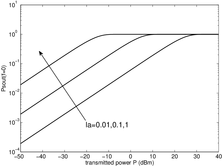
Figures 7 and 8 illustrate, respectively, the dependence of the outage probability $P_{\textrm{out}}^{\textrm{s}}(f)$ on the transmitted power $P$ and spatial density $\lambda$ of the emitting nodes. Specifically, as $P$ or $\lambda$ increase, the aggregate network emission becomes stronger, and thus $P_{\textrm{out}}^{\textrm{s}}(f)$ deteriorates at all frequencies, approaching the maximum value of 1.

We now extend the results to an heterogeneous scenario with $K$ different networks, where a given emitting node belongs to the network $k\in\{1\ldots K\}$ with probability $p_{k}$, independently of everything else. Using the splitting property of Poisson processes [26], we know the emitting nodes from each network $k$ form a spatial Poisson process, which is independent of the processes of other networks and has spatial density $\lambda_{k}=\lambda p_{k}$. Therefore, we can write the aggregate emission from all nodes in all networks as

where $\mathbf{Y}_{k}(t)=\sum_{i=1}^{\infty}\mathbf{Y}_{k,i}(t)$ is the aggregate emission from the individual network $k$, and

where $\mathbf{X}_{k,i}(t)$ and $\mathbf{h}_{k,i}(t,\tau)$ are, respectively, the transmitted signal and the impulse response of the multipath channel associated with node $i$ from network $k$. We consider that $\mathbf{X}_{k,i}(t)$ and $\mathbf{h}_{k,i}(t,\tau)$ are independent in both $k$ and $i$. Then, the aggregate emission $\mathbf{Y}_{k}(t)$ is also independent for different networks $k$ when conditioned on the positions $\mathcal{P}$, and thus $\mathcal{S}_{\mathbf{Y}}(f)=\sum_{k=1}^{K}\mathcal{S}_{\mathbf{Y}_{k}}(f).$ We can generalize (19) and write the conditional PSD of the aggregate emission $\mathbf{Y}(t)$ in this heterogeneous scenario as

where $\mathcal{D}_{\mathbf{h}_{k}}(f)$ and $\mathcal{S}_{\mathbf{X}_{k}}(f)$ are, respectively, the Doppler power spectrum and the PSD of the transmitted signal associated with network $k$; and the r.v.’s $\{A_{k}\}$ are i.i.d. in $k$ and given by

In (27), we have explicitly indicated the conditioning of $\mathcal{S}_{\mathbf{Y}}$ on the random node positions and shadowing $\mathcal{P}$. Since $A_{k}$ depends on $\mathcal{P}$, it can be seen as a r.v. whose distribution is skewed stable,

References

- [1] E. Sousa, “Performance of a spread spectrum packet radio network link in a Poisson field of interferers,” IEEE Trans. Inf. Theory, vol. 38, no. 6, pp. 1743–1754, 1992.
- [2] J. Ilow, D. Hatzinakos, and A. Venetsanopoulos, “Performance of FH SS radio networks with interference modeled as a mixture of Gaussian and alpha-stable noise,” IEEE Trans. Commun., vol. 46, no. 4, pp. 509–520, 1998.
- [3] X. Yang and A. Petropulu, “Co-channel interference modeling and analysis in a Poisson field of interferers in wireless communications,” IEEE Trans. Signal Process., vol. 51, no. 1, pp. 64–76, 2003.
- [4] S. Govindasamy, F. Antic, D. Bliss, and D. Staelin, “The performance of linear multiple-antenna receivers with interferers distributed on a plane,” in Proc. IEEE Workshop on Signal Process. Advances in Wireless Commun., 2005, pp. 880–884.
- [5] E. Salbaroli and A. Zanella, “A connectivity model for the analysis of a wireless ad hoc network in a circular area,” in Proc. IEEE Int. Conf. on Commun., June 2007, pp. 4937–4942.
- [6] A. Giorgetti, M. Chiani, and M. Z. Win, “The effect of narrowband interference on wideband wireless communication systems,” IEEE Trans. Commun., vol. 53, no. 12, pp. 2139–2149, Dec. 2005.
- [7] A. Giorgetti and D. Dardari, “The impact of OFDM interference on TH-PPM/BPAM transmission systems,” in Proc. IEEE Semiannual Veh. Technol. Conf., vol. 2, 2005, pp. 1037–1042.
- [8] P. C. Pinto and M. Z. Win, “Communication in a Poisson field of interferers - Part I: Interference distribution and error probability,” IEEE Trans. Wireless Commun., 2009, accepted pending revision.