Communication in a Poisson Field of Interferers – Part I: Interference Distribution and Error Probability

We model the spatial distribution of the nodes according to a homogeneous Poisson point process in the two-dimensional infinite plane. Typically, the terminal positions are unknown to the network designer a priori, so we may as well treat them as completely random according to a spatial Poisson process.¹¹ 1 The spatial Poisson process is a natural choice in such situation because, given that a node is inside a region $\mathcal{R}$, the probability density function (p.d.f.) of its position is conditionally uniform over $\mathcal{R}$. Then, the probability $\mathbb{P}\{n$ in $\mathcal{R}\}$ of $n$ nodes being inside a region $\mathcal{R}$ (not necessarily connected) depends only on the total area $\mathcal{A}$ of the region, and is given by [14]

where $\lambda$ is the (constant) spatial density of interfering nodes, in nodes per unit area. We define the interfering nodes to be the set of terminals which are transmitting within the frequency band of interest, during the time interval of interest, and hence are effectively contributing to the total interference. Then, irrespective of the network topology (e.g., point-to-point or broadcast) or multiple-access technique (e.g., time or frequency hopping), the above model depends only on the density $\lambda$ of interfering nodes.²² 2 Time and frequency hopping can be easily accommodated in this model, using the splitting property of Poisson processes [15] to obtain the effective density of nodes that contribute to the interference.

The proposed spatial model is depicted in Fig. 1. For analytical purposes, we assume there is a probe link composed of two nodes: the probe receiver, located at the origin of the two-dimensional plane (without loss of generality), and the probe transmitter (node $i=0$), deterministically located at a distance $r_{0}$ from the origin. All the other nodes ($i=1\ldots\infty$) are interfering nodes, whose random distances to the origin are denoted by $\{R_{i}\}_{i=1}^{\infty}$, where $R_{1}\leq R_{2}\leq\ldots$. Our goal is then to determine the effect of the interfering nodes on the probe link.

To account for the transmission characteristics of users, we consider that all interfering nodes employ the same linear modulation scheme, such as $M$-ary phase shift keying ($M$-PSK) or $M$-ary quadrature amplitude modulation ($M$-QAM), with symbol period $T$. Furthermore, they all transmit at the same power $P$ – a plausible constraint when power control is too complex to implement (e.g., decentralized ad-hoc networks). For generality, however, we allow the probe transmitter to employ an arbitrary linear modulation and arbitrary power $P_{0}$, not necessarily equal to those used by the interfering nodes.

We do not assume synchronization among interfering nodes, but instead consider asynchronous transmissions where different terminals are allowed to operate independently. As depicted in Fig. 2, node $i$ transmits with a random delay $D_{i}$ relative to node $0$, where $D_{i}\sim\mathcal{U}(0,T)$.³³ 3 We use $\mathcal{U}(a,b)$ to denote a real uniform distribution in the interval $[a,b]$. The probe receiver employs a conventional linear detector.⁴⁴ 4 Note that the other receiver nodes are not relevant for the analysis, since they do not cause interference. Typically, parameters such as the spatial density of interferers and the propagation characteristics of the medium (e.g., shadowing and path loss parameters) are unknown to the receiver. This lack of information about the interference, together with constraints on receiver complexity, justify the use of a simple linear detector, which is optimal when only AWGN is present.

To account for the propagation characteristics of the environment, we consider that the median of the signal amplitude decays with the distance $r$ according to $k/r^{b}$, for some given constant $k$. The amplitude loss exponent $b$ is environment-dependent, and can approximately range from $0.8$ (e.g., hallways inside buildings) to $4$ (e.g., dense urban environments), where $b=1$ corresponds to free space propagation [16].⁵⁵ 5 Note that the amplitude loss exponent is $b$, while the corresponding power loss exponent is $2b$. The use of such a decay law also ensures that interferers located far away have a negligible contribution to the total interference observed at the probe receiver, thus making the infinite-plane model reasonable.

To capture the shadowing effect, we model the channel amplitude gain $S$ as a log-normal random variable (r.v.) such that $S=\mu e^{\sigma G}$, where $G\sim\mathcal{N}(0,1)$,⁶⁶ 6 We use $\mathcal{N}(\mu,\sigma^{2})$ to denote a real Gaussian distribution with mean $\mu$ and variance $\sigma^{2}$. $\mu=k/r^{b}$ is the median of $S$, and $\sigma$ is the shadowing coefficient.⁷⁷ 7 This model for combined path loss and log-normal shadowing can be expressed in logarithmic form [17, 16], such that the channel loss in dB is given by $L_{\textrm{dB}}=k_{0}+k_{1}\log_{10}r+\sigma_{\textrm{dB}}G$, where $G\sim\mathcal{N}(0,1)$. The environment-dependent parameters $(k_{0},k_{1},\sigma_{\textrm{dB}}$) can be related to $(k,b,\sigma)$ as follows: $k_{0}=-20\log_{10}k$, $k_{1}=20b$, and $\sigma_{\textrm{dB}}=\frac{20}{\ln 10}\sigma$. The parameter $\sigma_{\textrm{dB}}$ is the standard deviation of the channel loss in dB (or, equivalently, of the received SNR in dB), and typically ranges from 6 to 12. Thus, the shadowing is responsible for random fluctuations of the channel gain around the median path gain $k/r^{b}$. The multipath effect is modeled as fast fading, which is superimposed on the path loss and shadowing. Specifically, the fading affects the received signal by introducing a random phase $\phi\sim\mathcal{U}(0,2\pi)$, as well as an amplitude factor $\alpha$ with arbitrary distribution and normalized to have unit power gain, i.e., $\mathbb{E}\{\alpha^{2}\}=1$.⁸⁸ 8 We use $\mathbb{E}\{\cdot\}$ and $\mathbb{V}\{\cdot\}$ to denote the expectation and variance operators, respectively. Because of its fast nature, the fading is always averaged out in this paper, both when determining the interference distribution and the error probability.

In what follows, we consider the shadowing (and similarly for the fading) to be independent for different nodes $i$, and approximately constant during at least one symbol interval. Additionally, the probe receiver can perfectly estimate the shadowing and fading affecting its own link, hence ensuring that coherent demodulation of the desired signal is possible.

Typically, the time variation of the distances $\{R_{i}\}_{i=1}^{\infty}$ of the interferers is highly coupled with that of the shadowing $\{G_{i}\}_{i=1}^{\infty}$ affecting those nodes. This is because the shadowing is itself associated with the movement of the nodes near large blocking objects. Thus, we introduce the notation $\mathcal{P}$ to denote “a particular realization of the distances $\{R_{i}\}_{i=1}^{\infty}$ and shadowing $\{G_{i}\}_{i=1}^{\infty}$ of the interferers,” or more succinctly, “the position of the interferers.” In this paper, we analyze the following two scenarios, which differ in the speed of variation of $\mathcal{P}$:

1. 1.

   Slow-varying $\mathcal{P}$: During the interval of interest (e.g., a symbol or packet time), the distance $R_{i}$ of each interferer is approximately constant, $R_{i}(t)\approx R_{i}$. Furthermore, the interferers have a long session lifetime, transmitting continuously over many symbols. In this quasi-static scenario, $\mathcal{P}$ varies slowly with time, and thus it is insightful to condition the interference analysis on a given realization of $\mathcal{P}$. As we shall see, this naturally leads to the derivation of the error outage probability of the probe link, which in this case is a more meaningful metric than the error probability averaged over $\mathcal{P}$ [18, 19, 20, 21].

2. 2.

   Fast-varying $\mathcal{P}$: As in the previous case, $R_{i}(t)\approx R_{i}$ during the interval of interest. However, the interferers have a short session lifetime, where each node periodically becomes active, transmits a burst of symbols, and then turns off (e.g., in a sensor or a packet network). Then, the set of interfering nodes (the set of nodes that are transmitting and contributing to the interference) changes often, and so does their effective position $\mathcal{P}$, which experiences a variation analogous to that of a block fading model. In this dynamic scenario, it is insightful to average the interference analysis over all possible realizations of $\mathcal{P}$, which naturally leads to the derivation of the average error probability of the probe link.

Under the system model described in Section II, the aggregate signal $Z(t)$ at the probe receiver can be written for $0\leq t\leq T$ as

where the first right-hand term is the desired signal from the transmitter probe node, $Y(t)$ is the aggregate interference with

and $W(t)$ is the AWGN with two-sided power spectral density $N_{0}/2$, and independent of $Y(t)$. In the above equations, we use the following the notation: $T$ is the symbol period; $f_{\mathrm{c}}$ is the carrier frequency; $a_{i}e^{j\theta_{i}}$ and $a_{i}^{\prime}e^{j\theta_{i}^{\prime}}$ are r.v.’s denoting successive constellation symbols transmitted by the node $i$ during the interval of interest $[0,T]$ (see Fig. 2); and $u(t)$ is the unit step function. The overall effect of the path loss, log-normal shadowing, and fading on node $i$ is captured by the amplitude factor $k\alpha_{i}e^{\sigma G_{i}}/R_{i}^{b}$, where $G_{i}\sim\mathcal{N}(0,1)$, and by the uniform phase $\phi_{i}$.⁹⁹ 9 Since we assume the probe receiver perfectly estimates the phase $\phi_{0}$ of the multipath fading affecting its own link, we can set $\phi_{0}=0$ without loss of generality. We consider that r.v.’s $\alpha_{i}$, $\phi_{i}$, $G_{i}$, $R_{i}$, $a_{i}e^{j\theta_{i}}$, $a_{i}^{\prime}e^{j\theta_{i}^{\prime}}$, and $D_{i}$ are mutually independent for a given node $i$, and that the sequences $\{\alpha_{i}\}$, $\{\phi_{i}\}$, $\{G_{i}\}$, $\{\mbox{$a_{i}e^{j\theta_{i}}$}\}$, $\{\mbox{$a_{i}^{\prime}e^{j\theta_{i}^{\prime}}$}\}$, and $\{D_{i}\}$ are independent identically distributed (i.i.d.) in $i$.

The probe receiver demodulates the desired signal from the aggregate signal $Z(t)$, using a conventional linear detector. This can be achieved by projecting $Z(t)$ onto the orthonormal set $\left\{\mbox{$\psi_{1}(t)=\sqrt{2/T}\cos(2\pi f_{\mathrm{c}}t)$},\right.$ $\left.\mbox{$\psi_{2}(t)=-\sqrt{2/T}\sin(2\pi f_{\mathrm{c}}t)$}\right\}$. Defining the in-phase and quadrature (IQ) components $Z_{n}=\int_{0}^{T}Z(t)\psi_{n}(t)dt$, $n=1,2$, we can write

where $W_{1}$ and $W_{2}$ are $\mathcal{N}(0,N_{0}/2)$ and mutually independent. After some algebra (Appendix A), $Y_{1}$ and $Y_{2}$ can be expressed as

where

Using complex baseband notation,¹⁰¹⁰ 10 Boldface letters are used to denote complex quantities; for example, $\mathbf{Z}=Z_{1}+jZ_{2}$. equations (1)-(5) can be further simplified as

where

and the distribution of $\mathbf{W}$ is given by¹¹¹¹ 11 We use $\mathcal{N}_{\textrm{c}}(0,\sigma^{2})$ to denote a circularly symmetric (CS) complex Gaussian distribution, where the real and imaginary parts are i.i.d. $\mathcal{N}(0,\sigma^{2}/2)$.

Since different interferers $i$ transmit asynchronously and independently, the r.v.’s $\{\mathbf{X}_{i}\}_{i=1}^{\infty}$ are i.i.d.

The distribution of the aggregate interference $\mathbf{Y}$ plays an important role in the evaluation of the error probability of the probe link. In what follows, we characterize such distribution in two important scenarios: the $\mathcal{P}$-conditioned and unconditional cases.

To derive the $\mathcal{P}$-conditioned distribution of the aggregate interference $\mathbf{Y}$ in (7)-(8), we start with the results given in [22]. This work shows that in the case of Rayleigh fading, an expression of the form of (8) can be well approximated by a circularly symmetric (CS) complex Gaussian r.v., such that

In [22], the validity of this approximation is justified both by analyzing the Kullback-Leibler divergence and comparing the error probabilities in the exact and approximated cases.¹²¹² 12 We can obtain (10) following another approach: if we consider that the interfering nodes are coded and operating close to capacity, then the signal transmitted by each interferer is Gaussian, such that $\mathbf{X}_{i}\sim\mathcal{N}_{\textrm{c}}(0,2V_{X})$ [23]. Then, conditioned on $\mathcal{P}$, the interference $\mathbf{Y}=\sum_{i=1}^{\infty}\frac{e^{\sigma G_{i}}\mathbf{X}_{i}}{R_{i}^{b}}$ becomes a sum of independent CS Gaussian r.v.’s and is therefore a CS Gaussian r.v. given by¹³¹³ 13 We use $X\,\mathop{\sim}\limits^{{\scriptscriptstyle|Y}}$ to denote the distribution of r.v. $X$ conditional on $Y$.

where $A$ is defined as

Furthermore, we show in [24] that after some algebra, $V_{X}$ can be expressed as

where $E\triangleq k^{2}\mathbb{E}\{a_{i}^{2}\}$ is the average symbol energy of each interfering node, measured $1\,\textrm{m}$ away from the interferer.¹⁴¹⁴ 14 Unless otherwise stated, we will simply refer to $E$ as the “average symbol energy” of the interferers. Because the r.v.’s $\{\mathbf{X}_{i}\}_{i=1}^{\infty}$ are i.i.d., $V_{X}$ does not depend on $i$ and is only a function of the interferers’ signal constellation. For the case of equiprobable symbols and a constellation that is symmetric with respect to the origin of the IQ-plane¹⁵¹⁵ 15 A constellation is said to be symmetric with respect to the origin if for every constellation point $(x,y)\in\mathbb{R}^{2}$, the point $(-x,-y)$ also belongs to the constellation. (e.g., $M$-PSK and $M$-QAM), the second right-hand term in (13) vanishes and $V_{X}=E/3$.

Lastly, note that since $A$ in (12) depends on the interferer positions $\mathcal{P}$ (i.e., $\{R_{i}\}_{i=1}^{\infty}$ and $\{G_{i}\}_{i=1}^{\infty}$), it can be seen as a r.v. whose value is different for each realization of $\mathcal{P}$. Furthermore, Appendix B shows that r.v. $A$ has a skewed stable distribution [25] given by¹⁶¹⁶ 16 We use $\mathcal{S}(\alpha,\beta,\gamma)$ to denote a real stable distribution with characteristic exponent $\alpha\in(0,2]$, skewness $\beta\in[-1,1]$, and dispersion $\gamma\in[0,\infty)$. The corresponding characteristic function is $$\phi(w)=\begin{cases}\exp\left[-\gamma|w|^{\alpha}\left(1-j\beta\mathrm{\,sign}(w)\tan\frac{\pi\alpha}{2}\right)\right],&\alpha\neq 1,\\ \exp\left[-\gamma|w|\left(1+j\frac{2}{\pi}\beta\mathrm{\,sign}(w)\ln|w|\right)\right],&\alpha=1.\end{cases}$$

where $b>1$, and $C_{x}$ is defined as

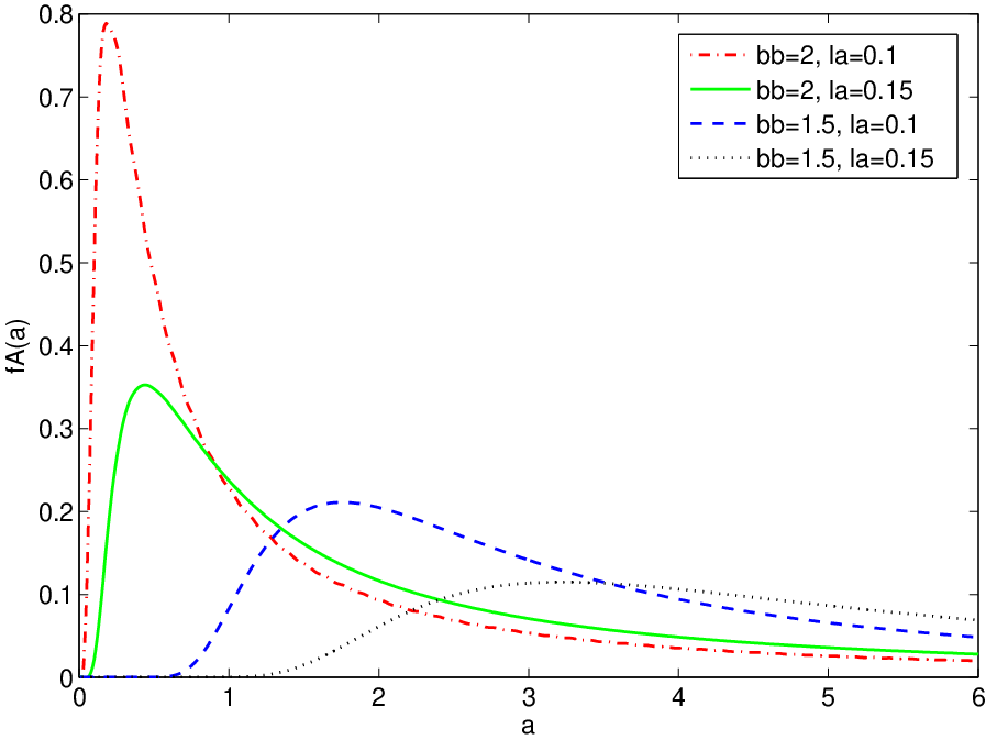
This distribution is plotted in Fig. 3 for different $b$ and $\lambda$.

To derive the unconditional distribution¹⁷¹⁷ 17 Unconditional in the sense of being averaged over the positions $\mathcal{P}$. of the aggregate interference $\mathbf{Y}$ in (7)-(8), we can show that sums of the form of (7) belong to the class of symmetric stable distributions [25]. This is because the r.v.’s $\{R_{i}\}_{i=1}^{\infty}$ correspond to distances in a spatial Poisson process and the $\{\mathbf{X}_{i}\}_{i=1}^{\infty}$ are i.i.d. and have a CS distribution. Specifically, Appendix C shows that $\mathbf{Y}$ has a CS complex stable distribution given by¹⁸¹⁸ 18 We use $\mathcal{S}_{\textrm{c}}(\alpha,\beta=0,\gamma)$ to denote a CS complex stable distribution with characteristic exponent $\alpha$ and dispersion $\gamma$, and whose characteristic function is $\phi(\mathbf{w})=\exp(-\gamma|\mathbf{w}|^{\alpha})$. Furthermore, the corresponding real and imaginary components are both $\mathcal{S}(\alpha,\beta=0,\gamma)$.

where $b>1$, and $C_{x}$ is defined in (15). Using (4)-(5), we can further express $\mathbb{E}\{|X_{i,n}|^{2/b}\}$ in (16) as

For the particular case of Rayleigh fading, (17) reduces to $\mathbb{E}\{|X_{i,n}|^{2/b}\}=k^{2/b}\Gamma\!\left(1+\frac{1}{b}\right)\cdot\chi(b),$ where we have used the moment relation for the Rayleigh r.v.’s $\alpha_{i}$ [26]. Since different interferers $i$ transmit asynchronously and independently, the parameter $\chi(b)$ does not depend on $i$ and is only a function of the amplitude loss exponent $b$ and the interferers’ signal constellation. Table I provides some numerical values for $\mathbb{E}\{|X_{i,n}|^{2/b}\}$.

The results of this section have to be interpreted carefully, because of the different types of conditioning involved. In the unconditional case, we let $\mathcal{P}$ be random, i.e., we let $\{R_{i}\}_{i=1}^{\infty}$ be the random outcomes of an underlying spatial Poisson process, and $\{G_{i}\}_{i=1}^{\infty}$ be the random shadowing affecting each interferer. Then, the unconditional interference $\mathbf{Y}$ is exactly stable-distributed and given by (16). We note that (16) and (17) hold for a broad class of fading distributions, in addition to Rayleigh fading. In the $\mathcal{P}$-conditioned case, the positions of the interferers are fixed. Then, $A$ in (12) is also a fixed number, and the interference $\mathbf{Y}$ is approximately CS Gaussian with total variance $2AV_{X}$, as given in (11).

In the quasi-static scenario of slow-varying $\mathcal{P}$, it is insightful to analyze the error probability conditioned on a given realization $\mathcal{P}$ of the distances $\{R_{i}\}_{i=1}^{\infty}$ and shadowing $\{G_{i}\}_{i=1}^{\infty}$ associated with the interferers, as well as on the shadowing $G_{0}$ of the probe transmitter. We denote this conditional symbol error probability by $P_{\textrm{e}}(G_{0},\mathcal{P})$.¹⁹¹⁹ 19 The notation $P_{\textrm{e}}(X,Y)$ is used as a shorthand for $\mathbb{P}\{\textrm{error}|X,Y$}.

To derive the conditional error probability, we employ the results of Section III-B for the $\mathcal{P}$-conditioned distribution of the aggregate interference $\mathbf{Y}$. Specifically, using (9) and (11), the received signal $\mathbf{Z}$ in (6) can be rewritten as

where

and $A$ was defined in (12). Our framework has thus reduced the analysis to a Gaussian problem, where the combined noise $\mathbf{\widetilde{W}}$ is Gaussian when conditioned on the location of the interferers.

The corresponding error probability $P_{\textrm{e}}(G_{0},\mathcal{P})$ can be found by taking the well-known error probability expressions for coherent detection of linear modulations in the presence of AWGN and fast fading [27, 28, 29, 30], but using $2AV_{X}+N_{0}$ instead of $N_{0}$ for the total noise variance. Note that this substitution is valid for any linear modulation, allowing the traditional results to be extended to include the effect of network interference. For the case where the probe transmitter employs an arbitrary signal constellation in the IQ-plane and the fading is Rayleigh-distributed, the conditional symbol error probability $P_{\textrm{e}}(G_{0},\mathcal{P})$ is given by

where

is the received signal-to-interference-plus-noise ratio (SINR), averaged over the fast fading; $M$ is the constellation size; $\{p_{k}\}_{k=1}^{M}$ are the symbol probabilities; $\mathcal{B}_{k}$, $\phi_{k,l}$, $w_{k,l}$, and $\psi_{k,l}$ are the parameters that describe the geometry of the constellation (see Fig. 4); $E_{0}\triangleq k^{2}\mathbb{E}\{a_{0}^{2}\}$ is the average symbol energy of the probe transmitter, measured $1\,\textrm{m}$ away from the transmitter; $A$ is defined in (12) and distributed according to (14); and $V_{X}$ is given in (13). When the probe transmitter employs $M$-PSK and $M$-QAM modulations with equiprobable symbols, (20) is equivalent to²⁰²⁰ 20 In this paper, we implicitly assume that $M$-QAM employs a square signal constellation with $M=2^{n}$ points ($n$ even).

and

respectively, where the integral $\mathcal{I}_{A}(x,g)$ is given by

In the general expression given in (20) and (21), the network interference is accounted for by the term $2AV_{X}$, where $A$ depends on the spatial distribution of the interferers and propagation characteristics of the medium, while $V_{X}$ depends on the interferer transmission characteristics. Since $2AV_{X}$ simply adds to $N_{0}$, we conclude that the effect of the interference on the error probability is simply an increase in the noise level, a fact which is intuitively satisfying. Furthermore, note that the modulation of the interfering nodes only affects the term $V_{X}$, while the (possibly different) modulation of the probe transmitter affects the type of error probability expression, leading to forms such as (22) or (23).

In our quasi-static model, the conditional error probability in (20) is seen to be a function of the slow-varying user positions and shadowing (i.e., $G_{0}$ and $\mathcal{P}$). Since these quantities are random, the error probability itself is a r.v. Then, with some probability, $G_{0}$ and $\mathcal{P}$ are such that the error probability of the probe link is above some target $p^{*}$. The system is said to be in outage, and the error outage probability is

In the case of slow-varying user positions, the error outage probability is a more meaningful metric than the error probability averaged over $\mathcal{P}$.

In the dynamic scenario of fast-varying $\mathcal{P}$, it is insightful to average the error probability over all possible realizations of interferer positions $\mathcal{P}$. We denote this average symbol error probability by $P_{\textrm{e}}(G_{0})$. Note that we choose not to average out the shadowing $G_{0}$ affecting the probe transmitter, since we have assumed the probe transmitter node is immobile at a deterministic distance $r_{0}$ from the probe receiver, and thus $G_{0}$ is slow-varying.

To derive the average error probability, we use the decomposition property of stable r.v.’s [25], which allows $\mathbf{Y}$ in (16) to be decomposed as

where $B$ and $\mathbf{G}$ are independent r.v.’s, and

with $\mathbb{E}\{|X_{i,n}|^{2/b}\}$ given in (17). Conditioning on the r.v. $B$, we then use (9) and (26) to rewrite the aggregate received signal $\mathbf{Z}$ in (6) as

where

Again, our framework has reduced the analysis to a Gaussian problem, where the combined noise $\mathbf{\widetilde{W}}$ is a Gaussian r.v. Note that this result was derived without resorting to any approximations – in particular, the Gaussian approximation of (10) was not needed here. We merely used the decomposition property of symmetric stable r.v.’s.

The corresponding error probability $P_{\textrm{e}}(G_{0})$ can be found by taking the error expressions for coherent detection in the presence of AWGN and fast fading, then using $2BV_{G}+N_{0}$ instead of $N_{0}$ for the total noise variance, and lastly (unlike in Section IV-A) averaging over the r.v. $B$. For the case where the probe transmitter employs an arbitrary signal constellation in the IQ-plane and the fading is Rayleigh-distributed, the average symbol error probability $P_{\textrm{e}}(G_{0})$ is given by

where

$B$ is distributed according to (27); $V_{G}$ is given in (28); and the other parameters have the same meaning as in Section IV-A. When the probe transmitter employs $M$-PSK and $M$-QAM modulations with equiprobable symbols, (20) is equivalent to

and

respectively, where the integral $\mathcal{I}_{B}(x,g)$ is given by

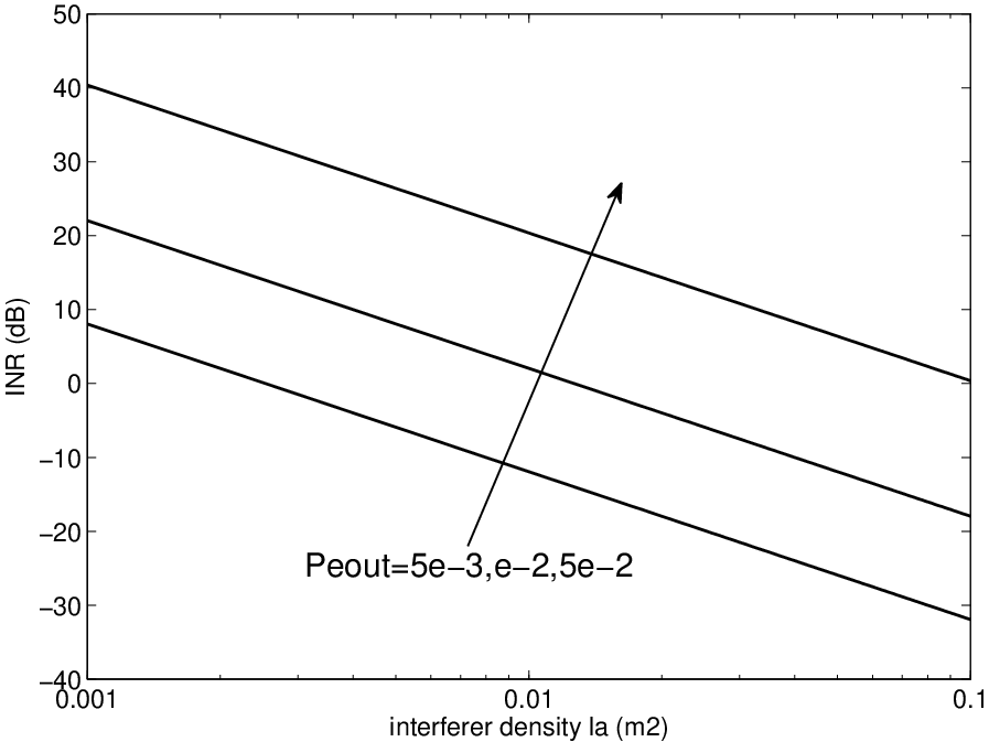
Using the results derived in Sections IV-A and IV-B, we can now analyze the dependence of the error performance on the density $\lambda$ and the average symbol energy $E$ of the interfering nodes. For that purpose, we use (20), although (30) would lead to similar conclusions. In (20), the error probability $P_{\textrm{e}}(G_{0},\mathcal{P})$ implicitly depends on parameters $\lambda$ and $E$ through the product $AV_{X}$ in the denominator of $\eta_{A}$ in (21). This is because the dispersion parameter $\gamma_{A}$ of the stable r.v. $A$ depends on $\lambda$ according to (14), and $V_{X}$ is proportional to $E$ as in (13). The dependence on $\lambda$ can be made evident by using the scaling property of stable r.v.’s [25] to write $AV_{X}=\lambda^{b}\widetilde{A}V_{X}$, where $\widetilde{A}$ is a normalized version of $A$, independent of $\lambda$. We thus conclude that the interference term $AV_{X}$ is proportional to $\lambda^{b}E$, where $b>1$. Clearly, the error performance degrades faster with an increase in the density of interferers than with an increase in their transmitted power. The tradeoff between $E$ and $\lambda$ for a fixed error performance is illustrated in Fig. 5.

Figs. 6 and 7 quantify the average and outage probabilities for several scenarios, showing their dependence on various parameters involved, such as the signal-to-noise ratio $\mathsf{SNR}=E_{0}/N_{0}$, interference-to-noise ratio $\mathsf{INR}=E/N_{0}$, amplitude loss exponent $b$, interferer spatial density $\lambda$, and link length $r_{0}$.

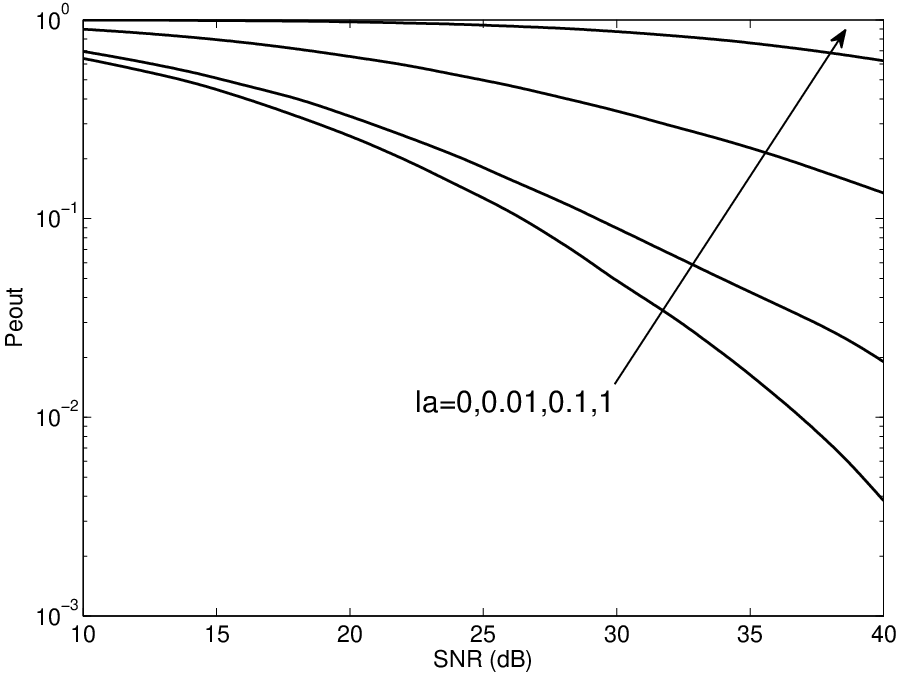
The plots of $P_{\textrm{out}}^{\textrm{e}}$ and $P_{\textrm{e}}(G_{0})$ presented here are of semi-analytical nature. Specifically, we resort to a hybrid method where we employ the analytical results given in (20)-(25) and (30)-(34), and perform a Monte Carlo simulation with respect to the stable r.v.’s (i.e., $A$ and $B$), according to [31]. Nevertheless, we emphasize that the expressions derived in this paper completely eliminate the need for simulation of the interferers’ position and waveforms in the network, in order to obtain the error performance.

For illustration purposes, the plots assume that all terminals (i.e., the probe transmitter and interfering nodes) use BPSK modulation. We analyze both cases of slow and fast-varying interferer positions $\mathcal{P}$, concurrently with the following two different scenarios:

1. 1.

   Heterogeneous network: The probe transmitter is allowed to use an arbitrary power $P_{0}=E_{0}/T$, not necessarily equal to the common power of the interfering nodes $P=E/T$, and hence $\mathsf{SNR}\neq\mathsf{INR}$ in general. This scenario is useful when the goal is to evaluate the impact of aggregate interference from a large number of identical secondary users (e.g., cognitive-radio terminals) on the performance of a primary link.

2. 2.

   Homogeneous network: The probe transmitter and interfering nodes all use the same power, and thus $\mathsf{SNR}=\mathsf{INR}$. This may correspond to a sensor network scenario, where there is a large number of indistinguishable, spatially scattered nodes with similar transmission characteristics. In such a case, the goal is to evaluate the impact of the aggregate network self-interference on the performance of each sensor node.

For the heterogeneous case depicted in Fig. 6, we conclude that the error performance deteriorates as $\lambda$ or INR increase, for a fixed SNR. This is expected because as the density or transmitted energy of the interferers increase, the aggregate interference at the probe receiver becomes stronger. Note, however, that in the homogeneous case where $\mathsf{SNR}=\mathsf{INR}$, the error performance improves as we increase the common transmitted power $P$ of the nodes (or equivalently, the SNR), although the gains become marginally small as $P\rightarrow\infty$ (see Fig. 7(b)). This happens because in the interference-limited regime where $\mathsf{SNR}=\mathsf{INR}\gg 1$, the noise term $N_{0}$ in (21) or (31) becomes irrelevant, and so the SNR in the numerator cancels with the INR in the denominator, making the performance independent of the transmitted power $P$.

The effect of the amplitude loss exponent $b$ on the error performance, on the other hand, is non-trivial. As illustrated in Fig. 7(a), an increase in $b$ may degrade or improve the performance, depending on the value of the link length $r_{0}$ and other parameters. This is because $b$ simultaneously affects both the received signal of interest and the aggregate interference – the former, through the term $1/r_{0}^{b}$; and the latter, through $\alpha_{A}$ and $\gamma_{A}$ in (14), or through $\alpha_{B}$, $\gamma_{B}$, and $V_{G}$ in (27) and (28).

References

- [1] A. J. Viterbi and I. M. Jacobs, “Advances in coding and modulation for noncoherent channels affected by fading, partial band, and multiple-access interference,” in Advances in Communication Systems: Theory and Applications, vol. 4. New York: Academic Press Inc., 1975, pp. 279–308.
- [2] E. Sousa, “Performance of a spread spectrum packet radio network link in a Poisson field of interferers,” IEEE Trans. Inf. Theory, vol. 38, no. 6, pp. 1743–1754, 1992.
- [3] J. Ilow, D. Hatzinakos, and A. Venetsanopoulos, “Performance of FH SS radio networks with interference modeled as a mixture of Gaussian and alpha-stable noise,” IEEE Trans. Commun., vol. 46, no. 4, pp. 509–520, 1998.
- [4] X. Yang and A. Petropulu, “Co-channel interference modeling and analysis in a Poisson field of interferers in wireless communications,” IEEE Trans. Signal Process., vol. 51, no. 1, pp. 64–76, 2003.
- [5] E. Salbaroli and A. Zanella, “A connectivity model for the analysis of a wireless ad hoc network in a circular area,” in Proc. IEEE Int. Conf. on Commun., June 2007, pp. 4937–4942.
- [6] B. Glance and L. Greenstein, “Frequency-selective fading effects in digital mobile radio with diversity combining,” IEEE Trans. Commun., vol. 31, no. 9, pp. 1085–1094, 1983.
- [7] A. Giorgetti, M. Chiani, and M. Z. Win, “The effect of narrowband interference on wideband wireless communication systems,” IEEE Trans. Commun., vol. 53, no. 12, pp. 2139–2149, Dec. 2005.
- [8] A. Giorgetti, M. Chiani, and D. Dardari, “Coexistence issues in cognitive radios based on ultra-wide bandwidth systems,” in Proc. IEEE Int. Conf. on Cognitive Radio Oriented Wireless Networks and Commun., Mykonos, GREECE, June 2006.
- [9] P. C. Pinto and M. Z. Win, “Communication in a Poisson field of interferers,” in Proc. Conf. on Inform. Sci. and Sys., Princeton, NJ, Mar. 2006, pp. 432–437.
- [10] ——, “Spectral characterization of wireless networks,” IEEE Wireless Commun. Mag., vol. 14, no. 6, pp. 27–31, Dec. 2007, special Issue on Wireless Sensor Networking.
- [11] P. C. Pinto, C.-C. Chong, A. Giorgetti, M. Chiani, and M. Z. Win, “Narrowband communication in a Poisson field of ultrawideband interferers,” in Proc. of IEEE Int. Conf. on Ultra-Wideband (ICUWB), Waltham, MA, Sept. 2006, pp. 387–392.
- [12] M. Z. Win, P. C. Pinto, A. Giorgetti, M. Chiani, and L. A. Shepp, “Error performance of ultrawideband systems in a Poisson field of narrowband interferers,” in Proc. IEEE Int. Symp. on Spread Spectrum Techniques & Applications, Manaus, BRAZIL, Aug. 2006, pp. 410–416.
- [13] P. C. Pinto and M. Z. Win, “Communication in a Poisson field of interferers - Part II: Channel capacity and interference spectrum,” IEEE Trans. Wireless Commun., 2009, accepted pending revision.
- [14] J. Kingman, Poisson Processes. Oxford University Press, 1993.
- [15] D. P. Bertsekas and J. N. Tsitsiklis, Introduction to Probability. Athena Scientific, 2002.
- [16] A. Goldsmith, Wireless Communications. Cambridge University Press, 2005.
- [17] G. L. Stüber, Principles of Mobile Communication. Springer, 2000.
- [18] O. Andrisano, V. Tralli, and R. Verdone, “Millimeter waves for short-range multimedia communication systems,” Proc. IEEE, vol. 86, no. 7, pp. 1383–1401, 1998.
- [19] A. Conti, M. Z. Win, and M. Chiani, “Invertible bounds for -QAM in fading channels,” IEEE Trans. Wireless Commun., vol. 4, no. 5, pp. 1994–2000, Sept. 2005.
- [20] ——, “On the inverse symbol error probability for diversity reception,” IEEE Trans. Commun., vol. 51, no. 5, pp. 753–756, May 2003.
- [21] A. Conti, M. Z. Win, M. Chiani, and J. H. Winters, “Bit error outage for diversity reception in shadowing environment,” IEEE Commun. Lett., vol. 7, no. 1, pp. 15–17, Jan. 2003.
- [22] A. Giorgetti and M. Chiani, “Influence of fading on the Gaussian approximation for BPSK and QPSK with asynchronous cochannel interference,” IEEE Trans. Wireless Commun., vol. 4, no. 2, pp. 384–389, 2005.
- [23] G. J. Foschini, “Private conversation,” AT&T Labs-Research, May 2007.
- [24] P. C. Pinto, “Communication in a Poisson Field of Interferers,” Master’s thesis, Department of Electrical Engineering and Computer Science, Massachusetts Institute of Technology, Cambridge, MA, Dec. 2006, thesis advisor: Professor Moe Z. Win.
- [25] G. Samoradnitsky and M. Taqqu, Stable Non-Gaussian Random Processes. Chapman and Hall, 1994.
- [26] J. Proakis, Digital Communications. McGraw-Hill, 2000.
- [27] M. Z. Win and J. H. Winters, “Virtual branch analysis of symbol error probability for hybrid selection/maximal-ratio combining in Rayleigh fading,” IEEE Trans. Commun., vol. 49, no. 11, pp. 1926–1934, Nov. 2001.
- [28] M. K. Simon and M.-S. Alouini, Digital Communication over Fading Channels. Wiley-IEEE Press, 2004.
- [29] J. W. Craig, “A new, simple and exact result for calculating the probability of error for two-dimensional signal constellations,” in Proc. Military Commun. Conf., Boston, MA, 1991, pp. 25.5.1–25.5.5.
- [30] W. M. Gifford, M. Z. Win, and M. Chiani, “Diversity with practical channel estimation,” IEEE Trans. Wireless Commun., vol. 4, no. 4, pp. 1935–1947, July 2005.
- [31] J. Chambers, C. Mallows, and B. Stuck, “A method for simulating stable random variables,” J. Amer. Statist. Assoc., vol. 71, pp. 340–344, 1976.
- [32] V. M. Zolotarev, One-Dimensional Stable Distributions. American Mathematical Society, 1986.